Characterising submonolayer deposition via visibility graphs

Abstract

We use visibility graphs as a tool to analyse the results of kinetic Monte Carlo (kMC) simulations of submonolayer deposition in a one-dimensional point island model. We introduce an efficient algorithm for the computation of the visibility graph resulting from a kMC simulation and show that from the properties of the visibility graph one can determine the critical island size, thus demonstrating that the visibility graph approach, which implicitly combines size and spatial data, can provide insights into island nucleation and growth processes.

I Introduction

Submonolayer deposition (SD) is a term used to describe the initial stages of thin film growth, such as during molecular beam epitaxy, where monomers are deposited onto a surface, diffuse and form large-scale structures (islands). Of particular interest is the mechanism for island nucleation, and how it is reflected in the statistical properties of the growing structures. SD is widely studied using kinetic Monte Carlo (kMC) simulations and it is recognised that under suitable conditions (described below), the statistical properties of the growing structures display scale invariance with distributions reflecting the underlying nucleation mechanism Amar .

Below we will be considering point islands, i.e. islands whose extent and internal structure have been neglected. We consider a one-dimensional model. Both these choices have been made for simplicity as the goal of the paper is a “proof of concept”, to demonstrate the ability of visibility graphs (VGs) to extract mechanism information from kMC. That said, point islands are often used in SD models, as they approximate SD accurately when the islands are “well separated” Mulheran1 . In the Conclusions sections we will discuss generalizations of our method to extended islands and to higher-dimensional settings. Our generalisation to extended islands requires a good understanding of the point island case and thus provides further motivation for using point island models.

Thus, we consider the situation where monomers are randomly deposited onto an initially empty one-dimensional lattice $L$ at a deposition rate of $F$ monolayers per unit time ($t$). The monomers diffuse at a rate $D$ and islands nucleate when $i+1$ monomers coincide at a lattice site. We call $i$ the critical island size. We assume no monomers can evaporate from the lattice and so the coverage $\theta$ can be defined as $\theta=100Ft\%$. $\theta$ is chosen large enough for us to be in the aggregation regime (where scale-invariance is found) i.e. where the monomers are much more likely to aggregate into islands than nucleate into new islands. The appropriate value of $\theta$ where the aggregation regime starts is dependent on $i$ and the ratio $R=D/F$.

Previous work on SD models has focused on the mean field densities, spatial distribution of islands or the size statistics of their islands (see Mulheran1 ; Mulheran2 ; Blackman ; Einax ; Evans for details) and the scaled gap and island size distributions for different critical island sizes $i$ illustrated in Figure 1 (for limited data). We define the gap between islands as the distance between two nucleated sites and the island size as the number of monomers at a particular site on the lattice (where the size of the island must be at least $i+1$). It is worth noting that spatial distributions and size statistics of islands are only negligibly affected by variations in the number of lattice sites $L$, by variations in $R$, or by the particular $\theta$ in the aggregation regime Blackman .

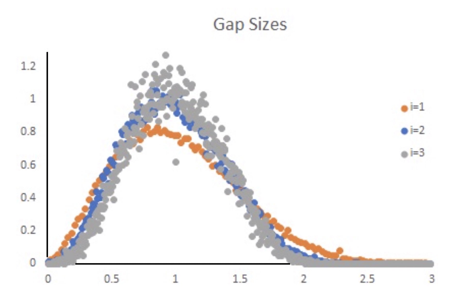
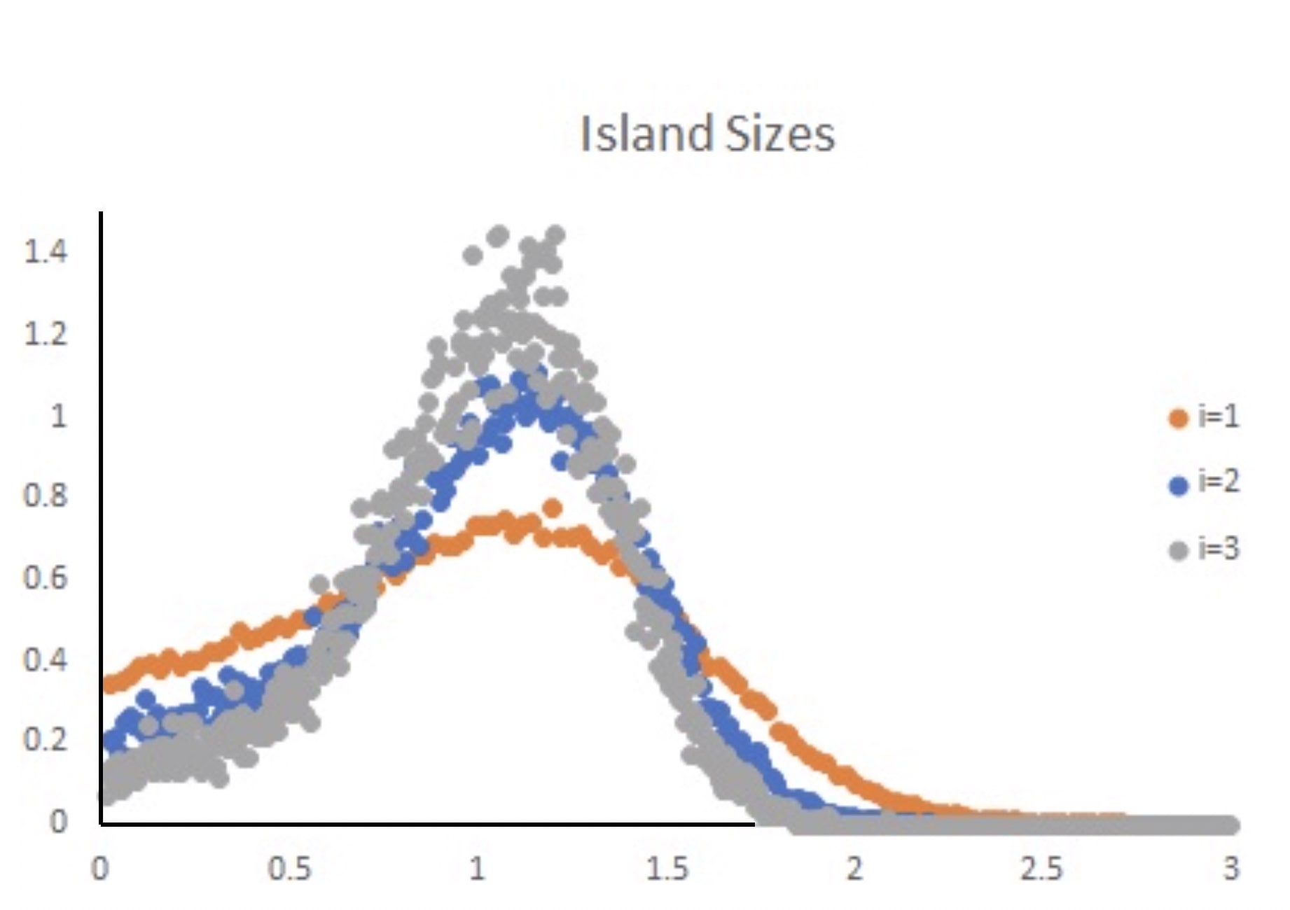
Figure 1: The scaled gap and island size distributions generated from kMC simulations on lattices with $L=10^{6}$ sites, with $R=10^{6}$ and up to coverage of $\theta=200\%$, where sizes are reported relative to the average, averaging results over 50 runs Mulheran1 .

One would like to combine the information contained in the spatial distribution of islands and in their size statistics. A suitable tool, which also allows higher-dimensional extensions which we discuss in the Conclusions section, is offered by VGs introduced by Lacasa et al. Lacasa originally to bring the tools of network theory to bear on time-series analysis. Subsequently, VGs have been used to analyse, among other things, exchange rate series Yang and to make solar cycle predictions Zou . Using VGs in the context of kMC simulations of SD allows us to apply complex network theory to SD. Here we develop an efficient algorithm for processing the data, and show how properties of the VG can be used to identify the critical island size from the island and gap size data.

Briefly, in a VG we connect each point $P$ with coordinates (location, size) (the top of our grey bars in Figure 2) to all other points that “are visible” from $P$ and analyse the resulting graph Lacasa .

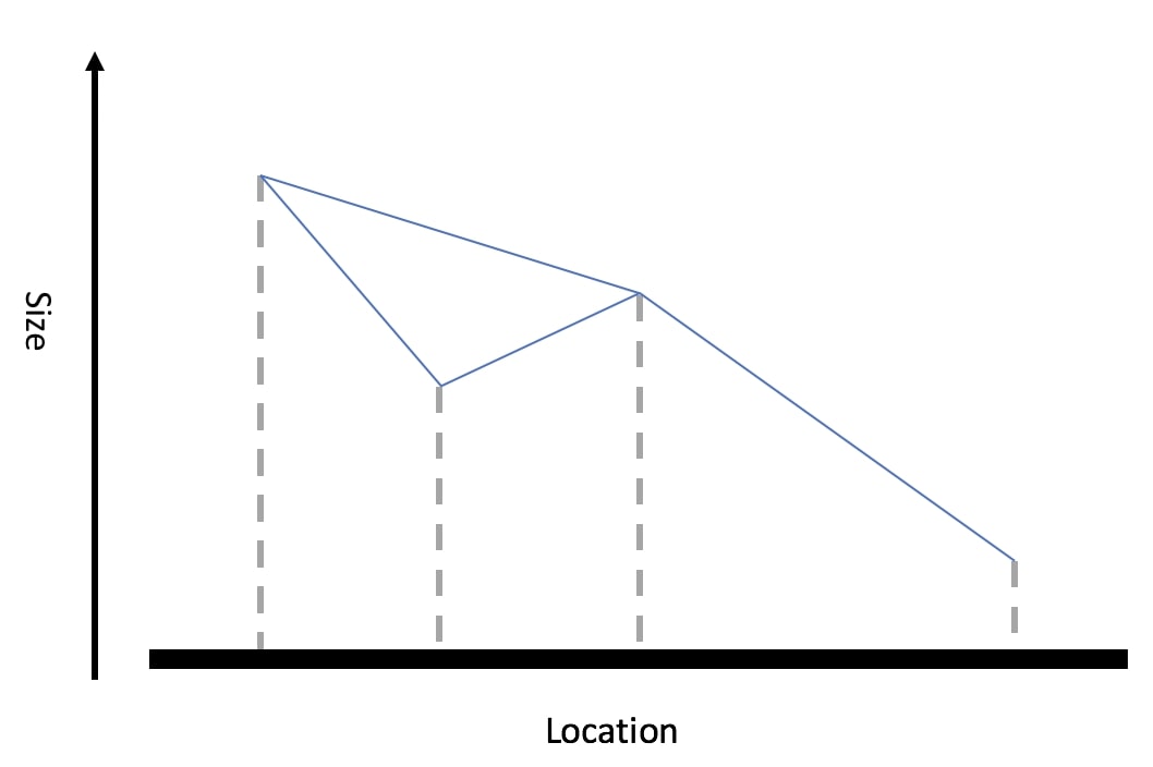
Figure 2: An example of a VG where the blue lines represent the edges in the network.

II The VG Algorithm

First, we would like to describe an efficient algorithm for the computation of a VG given $n$ points in the plane, $S=\{P_{1},P_{2},\ldots,P_{n}\}$, where $P_{j}=(x_{j},y_{j})$, $j\in\{1,\,\ldots,n\}$. The simplest way to construct the VG is by considering points $P_{a}$, $P_{b}\in S$ (assuming without loss of generality that $x_{a}<x_{b}$); then $P_{a}$ and $P_{b}$ are visible from each other if all points $P_{c}\in S$ such that $x_{a}<x_{c}<x_{b}$, satisfy

$$y_{c}<y_{b}+\dfrac{y_{b}-y_{a}}{x_{b}-x_{a}}(x_{c}-x_{b}).$$

To construct the VG we need to consider all two-point subsets of $S$, which gives us an algorithm with time complexity of $C=\frac{1}{6}n^{3}+\mathcal{O}(n^{2}).$ As our kMC simulations produce up to $10^{5}$ nucleated sites per simulation, this algorithm is impractical as one VG takes nearly two hours to produce on a single core desktop PC. Hence, we aim to find an algorithm that is faster than the naïve one.

We collect the results needed for the construction of such an algorithm in the following claims. Throughout, we let $P_{a},P_{b},P_{c}\in S$ be such that $x_{a}<x_{b}<x_{c}$.

Claim II.1

Let $A=(a_{jk})$ where $j,k\leq n$ be adjacency matrix of the VG. Then $a_{jj}=0,$ $a_{jj+1}=1$ when $j<n,$ $a_{jk}=a_{kj}.$

Claim II.2

Let $P_{a}$ and $P_{b}$ be connected and $y_{a}<y_{b}$. Then all points $P_{c}$ such that $y_{c}<y_{b}$ are not visible from $P_{a}$.

Claim II.3

Let $P_{a}$ be connected to $P_{b}$ and $P_{b}$ be connected to $P_{c}$. Then the slopes of the line segments connecting $P_{a}$ to $P_{b}$ and $P_{b}$ to $P_{c}$ are given by

$$m_{1}=\frac{y_{b}-y_{a}}{x_{b}-x_{a}}\>\>\text{and}\>\>m_{2}=\frac{y_{c}-y_{b}}{x_{c}-x_{b}},\>\text{respectively.}$$

Thus

1. if $m_{2}>m_{1}$, $P_{c}$ is visible from $P_{a}$,

2. if $m_{2}\leq m_{1}$, $P_{c}$ is not visible from $P_{a}$.

For two vectors $\bm{\mu}:=(\mu_{1},\mu_{2})$ and $\bm{\nu}:=(\nu_{1},\nu_{2})$ we define $\bm{\mu}\wedge\bm{\nu}:=\mu_{1}\nu_{2}-\mu_{2}\nu_{1}$.

Claim II.4

Let $P_{a}$ be connected to $P_{b}$ and define $\tilde{P_{c}}:=(x_{c},0)$. Then $P_{c}$ is visible from $P_{a}$ if and only if

$$t_{1}=\dfrac{|\bm{\gamma_{2}}\wedge\bm{\gamma_{1}}|}{\bm{\gamma_{2}}\cdot\bm{\gamma_{3}}}\in[0,\infty)\>\>\mbox{and }t_{2}=\>\>\dfrac{\bm{\gamma_{1}}\cdot\bm{\gamma_{3}}}{\bm{\gamma_{2}}\cdot\bm{\gamma_{3}}}\in[0,1],$$

where $\bm{\gamma_{1}}=P_{a}-P_{c}$, $\bm{\gamma_{2}}=\tilde{P_{c}}-P_{a}$, and $\bm{\gamma_{3}}=-(P_{b}(2)-P_{a}(2),P_{b}(1)-P_{a}(1))$, see Figure 3.

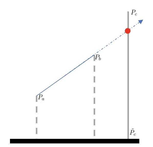
Figure 3: An illustration of (II.4)

II.1 New VG Algorithm

We can now use Claims (II.1)-(II.4) to construct our VG algorithm. We consider an arbitrary point $P_{j}\in S$ and the vector of elements to the right of the main diagonal in the $j$-th row of the adjacency matrix of the VG $[a_{j,j+1},\,a_{j,j+2},\ldots,\,a_{j,n}]$. Letting $2\leq k\leq n-j$ we have:

• $a_{j,j+1}=1$, by Claim (II.1).

• If $a_{j,j+k-1}=1$ and $y_{j+i}<y_{j+k-1}$ where $k\leq i\leq n-j$, then $a_{j,j+i}=0$ by Claim (II.2).

• If $a_{j,j+k-1}=1$ then $a_{j,j+k}=1$ if $m_{2}>m_{1}$ and $a_{j,j+k}=0$ otherwise by Claim (II.3).

• If $a_{j,j+k-1}=0$, then $a_{j,j+k}=1$ if $t_{1}\in[0,\infty)$ and $t_{2}\in[0,1]$ and $a_{j,j+k}=0$ otherwise by Claim (II.4).

We continue this process for all $P_{j}\in S$ and then use the final property from Claim (II.1) to complete our adjacency matrix.

Our new algorithm is around 15 times faster than the original and typically reduces computation time from two hours to eight minutes for the construction of a VG from one kMC run.

III Characterising the VG

Thus, we start with a kMC simulation of SD in one space dimension. Once the simulation is complete, we mark the location and the size (‘height’) of each nucleated island and construct the resulting VG.

Our simulations were performed on lattices with $L=10^{6}$ sites, $R=10^{6}$ up to coverage of $\theta=200\%$ for different critical island sizes $i$. (For $i=0$ we set the spontaneous nucleation probability i.e. the chance a monomer becomes fixed to the lattice to $p=10^{-6}$). We choose these conditions to guarantee we are in the aggregation regime and throughout the remainder of this paper we refer to these conditions as our ‘standard conditions’.

There are many ways to characterise a graph; these include criteria based on vertex degree, spectrum of the adjacency and other matrices defined from the graph, communicability and centrality indices Mieghem . Below we only analyse the vertex degree distribution and spectral gap in the adjacency matrix as these are sufficient to differentiate between VGs corresponding to different critical island sizes $i$. We discuss other possibilities of the method in the Conclusions section.

III.1 Degree Distribution

We begin our characterisation of the VG by considering the vertex degree distribution. Let $n$ be the number of nodes in our VG and $m(k)$ be the number of nodes in our visibility graph with $k$ connectivity; for simplicity we define $q(k):=m(k)/n$. The vertex degree distributions of VGs generated from kMC simulations (under our standard conditions) averaged over 50 simulations are shown in Figure 4.

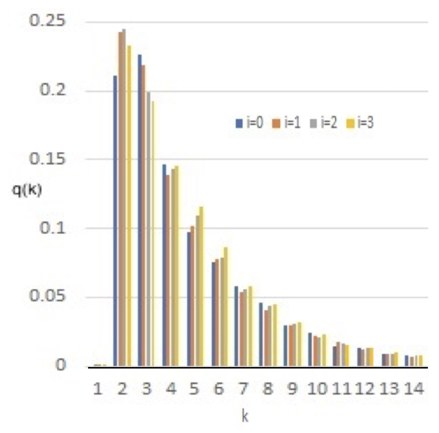
Figure 4: The vertex degree distributions of VGs generated from kMC simulations on lattices with $L=10^{6}$ sites, with $R=10^{6}$ and up to coverage of $\theta=200\%$ for $i=0,1,2$ and $3$ and in the $i=0$ case we let $p=10^{-6}$, averaging results over 50 runs.

From Figure 4, we see that graphs corresponding to different values of $i$ differ in the statistics of nodes having degree $k$, particularly when $3\leq k\leq 8$. To investigate this finding further, we consider this specific region as shown in Figure 5. To emphasise the differences we connect the points with straight lines.

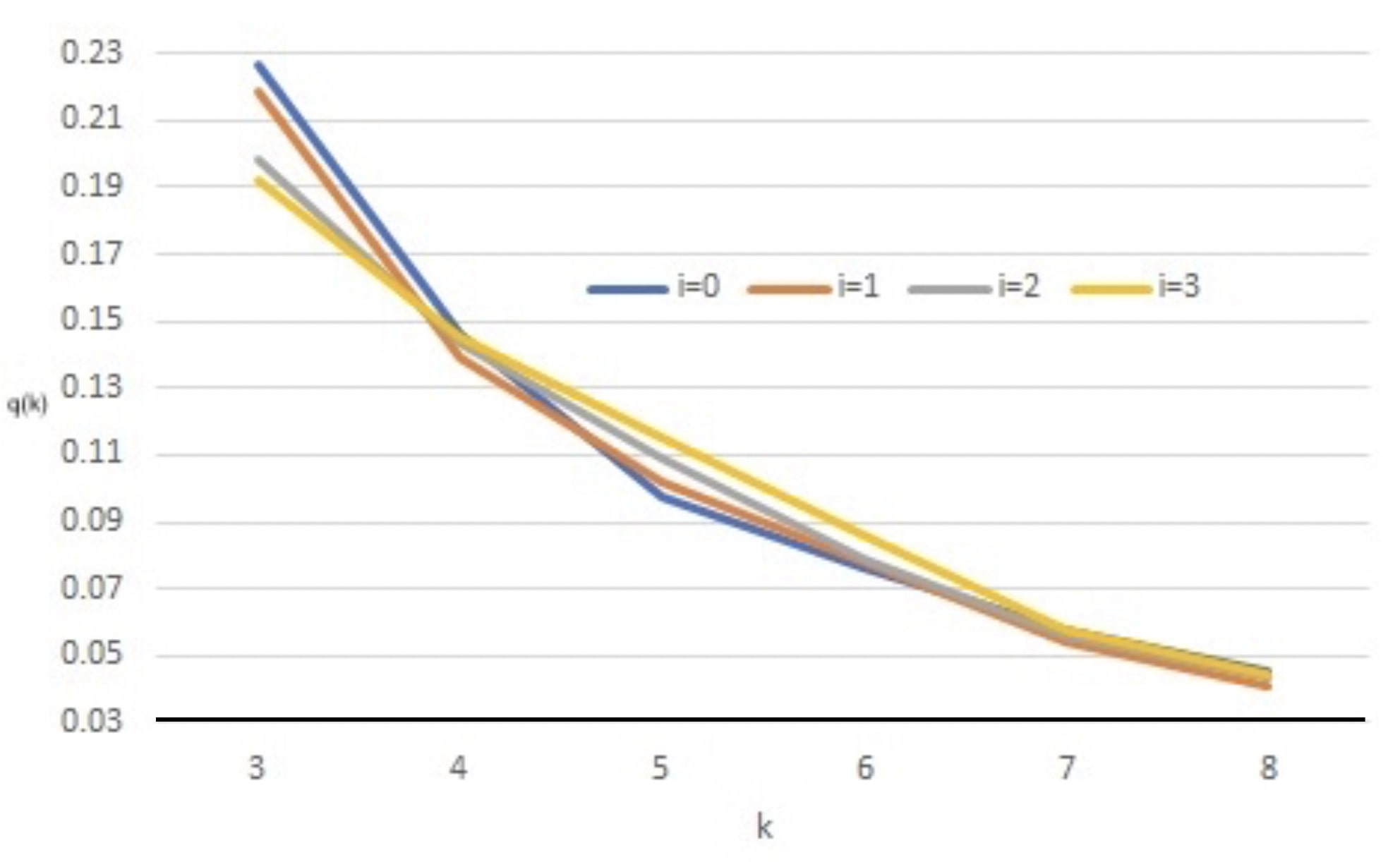
Figure 5: The vertex degree distributions of VGs generated from kMC simulations on lattices with $L=10^{6}$ sites, with $R=10^{6}$ and up to coverage of $\theta=200\%$ when $i=0,1,2$ and $3$ and in the $i=0$ case we let $p=10^{-6}$, averaging results over 50 runs, for $3\leq k\leq 8$.

As expected, for every $i$ considered, the degree distributions are exponential (see Allen for further details), however there are noticeable differences particularly for $q(3)$ for different $i$. Changes in $R$ (when $R=10^{7},10^{8}$ and $10^{9}$), $L$ (when $L=10^{7}$ and $10^{8}$) and $\theta$ (when $\theta=100\%$) have a negligible effect on the degree distributions confirming that we are operating in the aggregation (scaling) regime. This is consistent with the work on gap size, island size and spatial distributions, see Mulheran1 .

It is interesting to see whether the values for $q(3)$ can be used to identify the value of $i$. To do this, we generate a VG from a set of kMC simulations and generate $q(3)$ in each case. Our simulations were performed for values of $i=0,1,2,$ and $3$. We performed the process $50$ times, in each case testing whether $q(3)$ values alone can determine the value of i used to generate the kMC data. We found that $i$ was correctly predicted in $92\%$ of cases. In addition, in all cases the predicted $i$ was within $1$ of the true value of $i$.

III.2 Spectrum of the adjacency matrix

Next we consider the adjacency matrix of the VG. We consider the first five eigenvalues of the adjacency matrix of our VGs generated from kMC simulations under our standard conditions. As with the vertex degree distribution, we find consistent behaviour for each $i$. We average the eigenvalues over 50 runs, as shown in Figure 6.

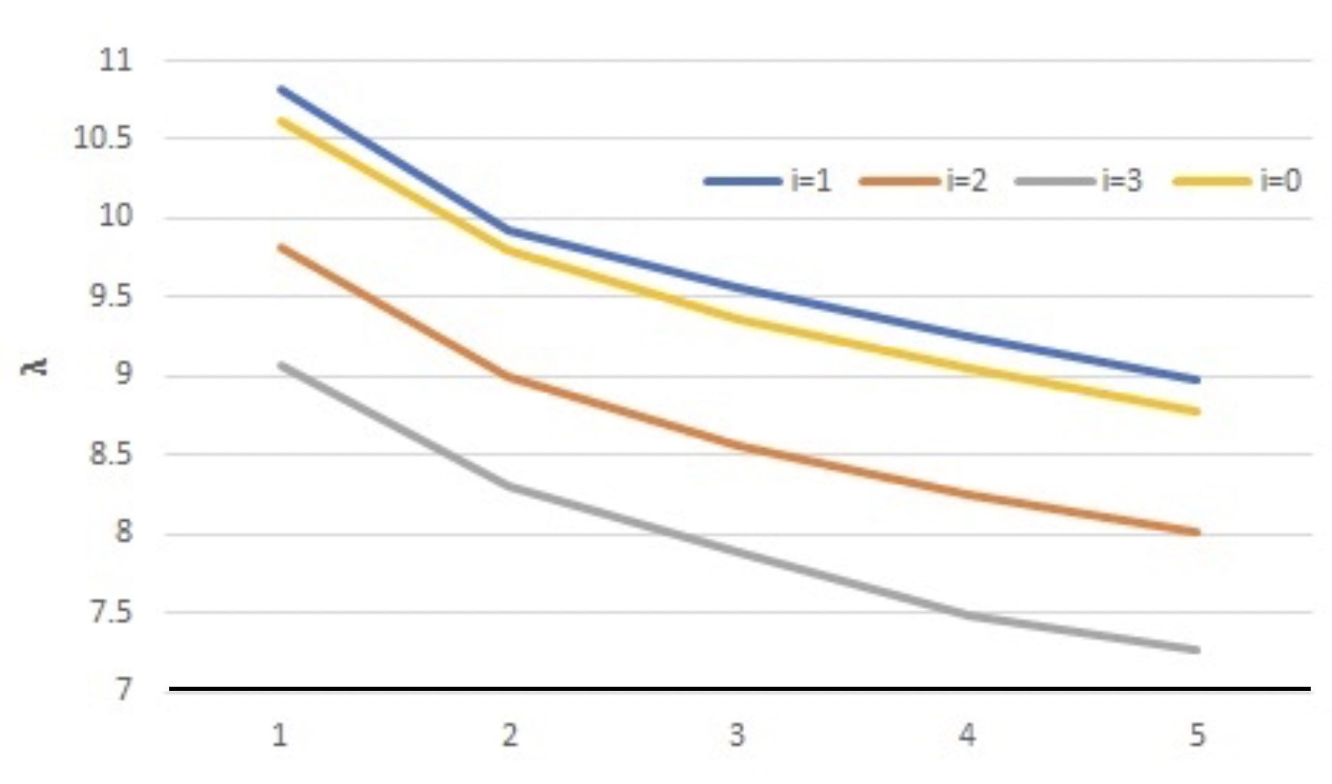
Figure 6: The eigenvalues of VGs generated from kMC simulations on lattices with $L=10^{6}$ sites, with $R=10^{6}$ and up to coverage of $\theta=200\%$ when $i=0,1,2$ and $3$ and in the $i=0$ case we let $p=10^{-6}$, averaging results over 50 runs.

As the $i=0$ case is practically indistinguishable from the $i=1$ case, to separate the two we consider the gap between the largest eigenvalue and the second largest eigenvalue of the adjacency matrix, i.e., the spectral gap, which has been shown to be related to the connectivity of the graph Mieghem ; these results are shown in Figure 7.

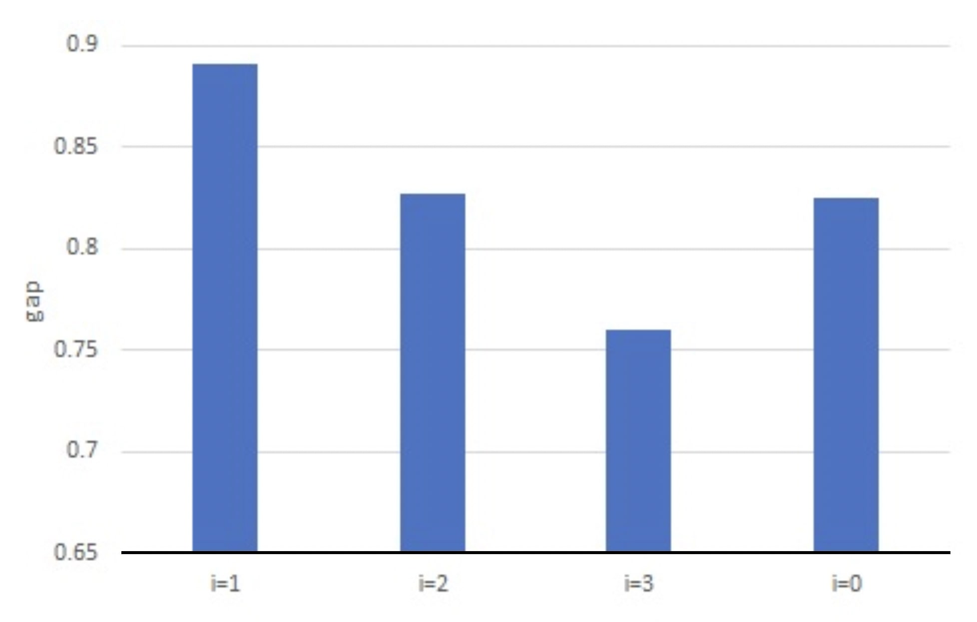
Figure 7: The gap between the first and second eigenvalue of the adjacency matrix from VGs generated from kMC simulations when $i=0,1,2$ and $3$, $R=16\times 10^{6}$, $L=10^{6}$, $\theta=200\%$ and in the $i=0$ we let $p=10^{-6}$, averaging results over 50 runs.

Once again, we find that changes in $R$, $L$ and $\theta$ have a negligible effect on the eigenvalues and the gap between the eigenvalues.

As in the case of using $q(3)$ to distinguish between nucleation mechanisms, we generate a VG from a kMC simulation under our operational conditions averaging results over 50 runs. In order to identify the value of $i$ from the adjacency matrix, we use the largest eigenvalue to separate the case of $i=2,3$ from the rest, and then the spectral gap to differentiate between $i=0$ and $i=1$. We performed this process 50 times. We found that $i$ was correctly predicted in all cases. Note, in contrast to Figure 1, the excellent separation of the $i=2$ and $i=3$ case.

IV Conclusions

We have shown that the analysis of some of the properties of the VG generated from a kMC simulation allows us to determine the underlying nucleation mechanism; both the degree distribution $(q(3))$ and the spectrum of the adjacency matrix allow us reliably to identify the value of $i$ used in the kMC simulation. We have also created an efficient algorithm for processing the kMC position/size data. Therefore, we have created an effective characterisation process that can be applied to experimental data for SD in one dimension, such as island nucleation and growth on a stepped substrate Pownall . This approach provides a way for the molecular scale rules for nucleation and growth to be decided.

The VG method has the potential to deal with more complicated mechanisms e.g. evaporation, mobile islands, unstable islands Allen1 , electric fields and any level of coverage within the scaling regime as discussed above. The generalisation of our work to extended islands is also straightforward, as we can create the vectors $P$ used in the construction of VG, by using the position of the centre of mass of an island and its mass as coordinates. We leave these versions of SD to future work.

It is true that at this stage there is no a priori reason why information about the critical island size $i$ should be contained in $q(3)$ or in the spectrum of the adjacency matrix, as demonstrated here. In general, assigning meaning to the spectrum of the adjacency matrix of a graph is difficult, as many different properties of the graph are stored in a single number, an eigenvalue. For a discussion of these issues, see Zenil . The VG framework used here falls in the domain of “equation-free” approaches (for a general philosophy of which see Kevrekidis ), as do the applications in complex (in particular, biological and financial) systems of topological data analysis Carlsson and Minkowski functionals Mecke . Such an exploratory study is necessary to verify, as we do here, that the tool is up to the task.

An important question is how to extend this methodology to two and three-space dimensions. In Lacasa2 a method is proposed to extend one-dimensional VGs to higher dimensions which enables the construction of VGs of large-scale spatially-extended surfaces. The method uses one-dimensional VGs along different straight lines in the multi-dimensional lattice to construct a single VG (only dependent on the number of lines one considers).

Of course, other ways of correctly identifying $i$ from data, such as from the scaled distribution of island sizes, already exist, and it is not clear whether a VG offers any immediate advantages in terms of robustness against noise or clarity of interpretation when the growth rules evolve over time. Nevertheless, we have successfully demonstrated that the VG approach usefully combines spatial and size data in a physically meaningful way, relating SD to network theory, thereby opening up new approaches to understanding more complex SD processes and their classification.

References

- (1) J. G. Amar and F. Family, Phys. Rev. Lett. 74, 2066 (1995).
- (2) P. A. Mulheran, K. P. O’Neill, M. Grinfeld and W. Lamb, Phys. Rev. E 86, 051606 (2012).
- (3) P. A. Mulheran and D. A. Robbie, Europhys. Lett. 49, 617 (2000).
- (4) J. Blackman, P. A. Mulheran, Phys. Rev. B 54 11681 (1996).
- (5) M. Einax, W. Dieterich, and P. Maass, Rev. Mod. Phys. 85, 921 (2013)
- (6) J. W. Evans, P. A. Thiel, M. C. Bartelt, Surface Science Reports 61, 1 (2006).
- (7) L. Lacasa, B. Luque, F. Ballesteros, J. Luque and J. C. Nuño, Proc. Nat. Acad. Sci. 105 4972 (2008).
- (8) Y. Yang, J. Wang, H. Yang and J. Mang, Phys. Rev. A 388 4431 (2009).
- (9) Y. Zou, M. Small, Z. H. Liu and J. Kurths, New J. Phys. 16 013051 (2014).
- (10) P. van Mieghem, Graph Spectra for Complex Networks, CUP, Cambridge 2011.
- (11) D. Allen, M.Grinfeld and R.Sasportes, J. Math. Anal. Appl. 472 1716 (2019).
- (12) D. Allen, Mathematical Aspects of Submonolayer Deposition, Ph. D. Thesis (in preparation), University of Strathclyde, Glasgow, UK 2019.
- (13) C. D. Pownall and P. A. Mulheran, Phys. Rev. B 60 9037 (1999).
- (14) H. Zenil, N. Kiani, and J. Tegnèr, in: Bioinformatics and Biomedical Engineering, I. Rojas and Francisco Ortuño eds., IWBBIO 2015, LNCS 9044, Springer, Chad 2015, pp. 395–405.
- (15) I. G. Kevrekidis, C. W. Gear and G. Hummer, AICHE J. 50 1346 (2004).
- (16) G. Carlsson, Acta Numerica 23 289 (2014).
- (17) C. Beisbart, R. Dahlke, K. Mecke and H. Wagner, in: Morphology and Geometry of Spatially Complex Systems, K. Mecke and D. Stoyan, eds., Springer-Verlag, Berlin 2002, pp. 238–260.
- (18) L. Lacasa and J. Iacovacci, Phys. Rev. E 96 012318 (2017).