The cosmic epoch dependence of environmental effects on size evolution of red-sequence early-type galaxies .

This work aims to observationally investigate the history of size growth of early-type galaxies and how the growth depends on cosmic epoch and the mass of the halo in which they are embedded. We carried out a photometric and structural analysis in the rest-frame $V$ band of a mass-selected ($\log M/M_{\odot}>10.7$) sample of red-sequence early-type galaxies with spectroscopic/grism redshift in the general field up to $z=2$ to complement a previous work presenting an identical analysis but in halos 100 times more massive and 1000 times denser. We homogeneously derived sizes (effective radii) fully accounting for the multi-component nature of galaxies and the common presence of isophote twists and ellipticity gradients. By using these mass-selected samples, composed of 170 red-sequence early-type galaxies in the general field and 224 identically selected and analyzed in clusters, we isolate the effect on galaxy sizes of the halo in which galaxies are embedded and its dependence on epoch. We find that the $\log$ of the galaxy size at a fixed stellar mass, $\log M/M_{\odot}=11$, has increased with epoch at a rate twice as fast in the field than in cluster in the last 10 Gyr ($0.26\pm 0.03$ versus $0.13\pm 0.02$ dex per unit redshift). Red-sequence early-type galaxies in the general field reached the size of their cousins in denser environment by $z=0.25\pm 0.13$ in spite of being three times smaller at $z\sim 2$. Data point toward a model where size growth is epoch-independent (i.e., $\partial\log r_{e}/\partial z=c$), but with a rate $c$ depending on environment, $\partial c/\partial\log M_{halo}\approx 0.05$. Environment determines the growth rate ($d\log r_{e}/dz$) at all redshifts, indicating an external origin for the galaxy growth without any clear epoch where it ceases to have an effect. The larger size of early-type galaxies in massive halos at high redshift indicates that their size grew buildup earlier (at $z>2$) at an accelerated rate, slowing down at some still unidentified $z>2$ redshift. Instead, the size growth rate of red-sequence early-type galaxies in low-mass halos is reversed: it proceeds at an increased rate at late epochs after an early period ($z>2$) of reduced growth, in agreement with the qualitative hierarchical picture of galaxy evolution. We found similar values of scatter around the mass-size relation independently of environment and epoch, indicating that the amount of dissipation in the system forming the observed galaxy does not vary greatly with epoch or environment.

1 Introduction

The origin and evolution of galaxies are among the most intriguing and complex chapters in the formation of cosmic structures (verbatim from Madau & Dickinson 2014). Understanding galaxy evolution requires controlling cosmic time, environment, mass, halo growth history, AGN activity, and much more because likely a combination of these factors leads to the quenching of star formation and the emergence of the galaxy populations we see in the nearby Universe. In turn, galaxies live in dynamical environments where halo mass certainly plays a role in shaping their properties because the physical processes altering the star formation history and the size growth are likely fundamentally different for objects close to the bottom of the halo potential well and for those still orbiting in a much larger halo. In particular, does halo mass affect the size evolution of massive early-type galaxies? In a hierarchical galaxy formation model, halo mass assembly histories systematically differ in different environments, with sub-halos aggregating earlier in denser environments (e.g., Maulbetsch et al. 2006). Therefore, galaxy evolution is accelerated in dense environments, while early-type galaxies in less dense environments should catch up with their cousins in denser environments having experienced an earlier size growth. Semi-analytic models does not reproduce this expected behavior, however (see Sec 5.2). If instead secular processes are responsible for the size growth, then the growth should be environmental-independent.

The most effective way to put forward the effect of the halo is to compare galaxies in their own halo versus galaxies in halos of other galaxies, i.e., centrals versus satellites. Using an older terminology, this is a comparison of field versus cluster galaxies at a given galaxy mass when we want a large mass contrast between the accreting and primary halo.

Observational evidence about the environmental effects on size are conflicting or inconclusive and largely focus on the mere existence of a difference: some works suggest no environmental dependency (e.g., Rettura et al. 2010; Maltby et al. 2010; Valentinuzzi et al. 2010; Kelkar et al. 2015; Huertas-Company et al. 2013; Allen et al. 2015; Saracco et al. 2017), some others claim larger sizes in dense environments (e.g., Delaye et al. 2014; Lani et al. 2013; Yoon et al. 2017) or, in a few cases, suggest a reverse trend (e.g., Raichoor et al. 2011). In general, environmental studies based on surveys lack sensitivity because they do not include massive clusters (or, if present, they provide a minority of galaxies). Instead, environmental studies including clusters often lack sensitivity because of the limited sample size and/or redshift range probed, or often rely on field samples heterogeneously selected and analyzed.

Putting forward the effect of the halo is furthermore complicated by the heterogeneous nature of galaxies in terms of: a) colors (e.g., Sandage & Visvanathan 1978) and therefore star formation histories (e.g., Larson et al. 1980); b) morphologies (e.g., Hubble 1926) and therefore structure evolution (Dressler 1980); and, likely, c) stellar mass assembly history (e.g., Baugh et al. 1996). The heterogeneous nature of galaxies complicates the study of their evolution because of the not completely disjoint classes and of the difficulty of replicating the same classification at all redshifts. For example, while in the local Universe many works adopt the Hubble sequence, in high-redshift studies morphological classes may be replaced by large Sersic (1964) index, quiescence (e.g., Newman et al. 2012), or massiveness. Because of likely diverse evolutionary paths of the different classes (e.g., Moresco et al. 2013), a non-homogeneous selection at different redshifts is prone to systematics. Furthermore, even focusing on one single class may not suffice when composed of galaxies having likely heterogenous histories such as quiescent galaxies, known to be a composite population of truly passive galaxies, dusty star-forming galaxies (Williams et al. 2009; Moresco et al. 2013) and recently quenched galaxies (Carollo et al. 2013; Andreon et al. 2016).

To complicate the issue, galaxies are multi-component stellar systems (have arm, bars, bulges, disks, etc.), yet their half-light radii are almost always derived as if they were single systems (often fitting a single Sersic profile to the azimuthally averaged radial profile) which is prone to systematics and complicates the interpretation of the found trends.

Finally, the considered redshift may matter: studying a fixed redshift only, or a reduced range, may only reveal a part of the picture because halo mass may be important at one cosmic time and negligible at another, leading to apparently conflicting results.

In Andreon, Dong, & Raichoor (2016, Paper I) we derived half-light radii for cluster galaxies on the red sequence and of early-type morphology in the rest-frame $V$ band of 224 galaxies with $\log M/M_{\odot}\gtrsim 10.7$ at $0.02<z<1.80$. The analysis was based on HST imaging for all $z>0.03$ galaxies (i.e., with sufficient resolution) and allowed galaxies to be multi-component. We want to repeat here a fully homogeneous selection and analysis, but for field galaxies, to isolate the effect of the environment. With the data derived in this paper, we not only identify whether the halo has an effect on galaxy structure, but we also show how the halo influence depends on epoch. By comparing halos with masses from a few to several $10^{14}M_{\odot}$ (clusters) to halos hosting galaxies with stellar mass of $10^{11}M_{\odot}$, and hence total mass of $\approx 10^{12}M_{\odot}$ (van Huiter et al. 2011), we are comparing halos differing by two orders of magnitude in mass and three orders of magnitude in (central) density. A group versus field comparison would instead explore narrower ranges. In such a comparison, galaxies of a fixed mass, say $\log M/M_{\odot}=11$, will be all satellite in clusters (no brightest cluster galaxy is so light in the studied massive clusters), while almost all are central in the field (the few galaxies in groups with brighter/more massive galaxies have been removed in our study, see Sec. 2).

Throughout this paper, we assume $\Omega_{M}=0.3$, $\Omega_{\Lambda}=0.7$, and $H_{0}=70$ km s^-1 Mpc^-1. Magnitudes are in the AB system. We use the 2003 version of Bruzual & Charlot (2003) stellar population synthesis models with solar metallicity and a Salpeter initial mass function (IMF). We use stellar masses that count only the mass in stars and their remnants. For a single stellar population, or $\tau=0.1$ Gyr model, the evolution of the stellar mass between ages of 2 and 13 Gyr is about 5%. Therefore, comparisons (e.g., of radii) at a fixed present-day mass are degenerate with comparisons with mass at the time of the observations (see Andreon et al. 2006 for a different situation).

2 Data and sample selection

In this paper we want to mirror what was done for cluster galaxies, namely to derive sizes and masses for galaxies of early-type morphology (ellipticals and lenticulars) at $z<2$ with $\log M/M_{\odot}\gtrsim 10.7$ and on the red sequence when measured on a filter pair bracketing the $4000$ Å break.

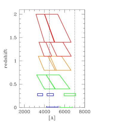
Figure 1: Rest-frame wavelength coverage of the filters used for measuring red sequence membership. The two blue bands at $z\sim 0.27$ are used to check the sensitivity of the selection on the blue band used, see text.

At $z>0.4$ we used GOODS-N and Hubble Legacy fields. At $0.25<z<0.3$ we used the larger (2 deg) COSMOS field, whereas at $25<D<42.9$ Mpc we used part of the SDSS DR12 (Alam et al. 2015). We excluded galaxies with $D<25$ Mpc to minimize the effects of peculiar motions, while the other redshift ranges were dictated by having an appropriate sampling in wavelength and resolution. In detail, at $z>0.4$ for photometry and morphological classification we used deep Wide Field Camera 3 near-infrared (NIR) and Advanced Camera for Survey (ACS, Sirianni et al. 2005) wide field camera imaging of the Hubble Legacy Field (including the shallower and narrower GOODS-S), distributed by Illingworth et al. (2016) and GOODS-N, distributed partly by CANDELS and partly by 3D-HST. We run SExtractor (Bertin & Arnouts 1996) in double imaging mode, using F160W for detection at $z>0.8$ and F850LP at lower redshift. Colors are based on fluxes within the detection isophote with a minor correction for PSF differences across filters (derived in Paper I). At $0.25<z<0.3$, we used 30-band matched photometry from Laigle et al. (2015). Laigle et al. (2015) gives photometry in the B, V, and R band rest-frame that we used for measuring colors. These bands are interpolated from the available filters closest to them. For sizes and masses we used instead HST F814W images. At $25<D<42.9$ Mpc, we drew galaxies from the complete sample of early-type galaxies in ATLAS3D (Cappellari et al. 2011, 2013). We used the SDSS catalog for colors and SDSS $r$ band images built from distributed frames for our own photometry, size measurements, and morphological classification.

Fig. 1 shows the rest-frame wavelength coverage of the filters used to determine whether the galaxy belongs to the red sequence. At all $z$ we similarly sampled the $4000$ Å break. At $0.25<z<0.3$ we used two blue bands to check the sensitivity to the adopted filter, and we found that the selected samples are virtually identical. To measure the half-size radius we used ACS or WFC3 images at $z>0.01$ ($F160W$, $F125W$, $F105W$, $F814W$, and $F814W$, from high to low redshift).

We applied luminosity and color cuts: we only considered galaxies brighter than a Bruzual & Charlot (2013) single stellar population with $\log M/M_{\odot}=10.7$ and $z_{f}=3$ because we are interested in $\log M/M_{\odot}\gtrsim 11$ galaxies. We then selected galaxies on the red sequence. We initially used a [-0.2,+0.2] mag range around the red sequence (at $1.4<z<2$ and $0.25<z<0.3$), later reduced to [-0.15,0.2] mag (other redshift ranges) because bluer galaxies turned out to be late-type galaxies (but cost operator time). At $25<D<42.9$ Mpc, $\log M/M_{\odot}>11.9$ galaxies are overly represented in the parental (ATLAS3D) sample, while they are absent in other samples. We therefore applied the additional cut $\log M/M_{\odot}<11.9$. Finally, we only retain elliptical and lenticular galaxies and compute sizes in a band sampling about 5000-6000 Å rest-frame, as detailed in Sec. 3.

Since we are studying either NGC galaxies or medium-bright galaxies in famous fields, virtually all galaxies have a spectroscopic redshift (or a distance measurement for galaxies in the very nearby Universe). Spectroscopy comes from grism/spectroscopic redshifts (and good photometry, use_phot=1) listed in 3D-HST (Skelton et al. 2014) at $z>0.4$, Laigle et al. (2015) at $0.25<z<0.3$, and from Cappellari et al. (2013 and references therein) at $25<D<42.9$ Mpc.

Concerning sample composition, we removed fainter galaxies of identified groups because we only want central galaxies, plus the central one for a few rich (crowded, to be precise) groups, both to widen the environmental range of our study and because the isophotal analysis in very crowded environments is unfeasible. As detailed in Appendix A, these bright and massive galaxies carry almost no information on $\log M/M_{\odot}\sim 11$ galaxies, which is the focus of this study, and therefore including or removing them from the sample is irrelevant for the quantity of our interest (independently of whether these galaxies should be removed or kept in principle).

Our sample is virtually uncontaminated and almost complete, and incompleteness mostly random and therefore benign, as detailed in Appendix A.

Images are much deeper than needed and indeed morphological classification and size measurements of many of the same galaxies have already been performed in the past using a reduced exposure time and down to fainter magnitudes (e.g., van der Wel et al. 2012; Cassata et al. 2011), but are recomputed here using deeper observational material, with improved methods, and using a more uniform sampling of the red band (used for size determination) for homogeneity with the cluster sample.

Table 1: Coordinates, masses, sizes, and PSF corrections.

ID	R.A.	Dec.	$\log M/M_{\odot}$	$\log r_{e}$	PSF corr
	J2000			[kpc]
$1.4<z<2.0$
12378	189.10034	62.15319	11.02	-0.31	-0.31
14579	189.19055	62.16169	10.87	-0.34	-0.33
17506	189.05850	62.17359	10.80	0.09	-0.12
…
$25<D<42.9$ Mpc
…
5854	226.94879	2.56856	10.87	0.22	0.00
5864	227.38980	3.05274	10.95	0.30	0.00
6278	255.20976	23.01096	11.14	0.30	0.00

Table 1 is entirely available in electronic form at the CDS. More digits than needed are reported for quantities.

3 Morphology, size, and stellar mass

As detailed in Paper I, in order to derive effective radii and total luminosities (used later to derive the galaxy mass) we fit the galaxy isophotes, precisely as done for galaxies in different environments at low and intermediate redshift (e.g., Michard 1985; Poulain et al. 1992; Michard & Marshall 1993, 1994; Andreon 1994; Andreon et al. 1996, 1997a,b, etc.) and high redshift (Paper I). Briefly, isophotes are decomposed in ellipses plus Fourier coefficients (Carter et al. 1978; Bender & Moellenhoff 1987, Michard & Simien 1988) to describe deviations from the perfect elliptical shape. We classify galaxies by detecting morphological components in the radial profiles of the isophote parameters. Such a quantitative classification is more reproducible than morphologies based on visual inspection (Andreon & Davoust 1997) and returns morphologies on average coincident with those performed by morphologists such as Hubble, Sandage, de Vaucouleurs, and Dressler (Michard & Marshall 1994; Andreon & Davoust 1997). By this morphological classification, we remove from the sample non-early-type galaxies (i.e., spirals and irregulars), only keeping elliptical and lenticular galaxies.

To compute the total galaxy flux, and from it the galaxy mass and size, the flux between isophotes is integrated up to the last detected isophote, in turn determining the curve of growth. To extrapolate it to infinity, we fit the measured growth curve with a library of growth curves measured for galaxies of different morphological types in the nearby universe (de Vaucouleurs 1977), keeping the one that fits best. The half-light isophote is, by definition, the isophote including half the total light. The half-light circularized radius, $r_{e}$, is defined as the square root of area included in the half-light isophote divided by $\pi$. This definition allows us to define the half-light radius whatever the isophote shapes are and irrespective of whether galaxies have a single value of ellipticity and position angle, or values that depend on radius, as barred galaxies, lenticulars, and many ellipticals have. Our approach directly addresses, and straightforwardly fix, the recently recognized problem represented by objects not well represented by the idealized objects with concentric ellipses of fixed ellipticity and position angle and with perfect Sersic profiles, assumed instead in most works, and for which a patch has been organized (Szomoru et al. 2010, 2013; Patel et al. 2017).

The background light is accounted for, and subtracted, by fitting a low-order polynomial to the region surrounding the studied galaxy, and accounting for the galaxy flux at large radii. This also allows us to remove any residual gradient present in the image, for example due to scattered light.

Masses of red-sequence early-type galaxies are derived from $\lambda\approx 6000$ Å  luminosities assuming our standard BC03 SSP model with $z_{f}=3$ (which in turn matches the red-sequence color) and checked for cluster galaxies in Paper I to introduce a negligible $0.10$ dex scatter in mass and no bias compared to a derivation based on fitting many photometric bands and $3000-6000$ Å spectroscopy. Further checks are given in Sec. 4.1.3.

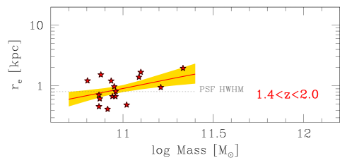
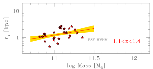
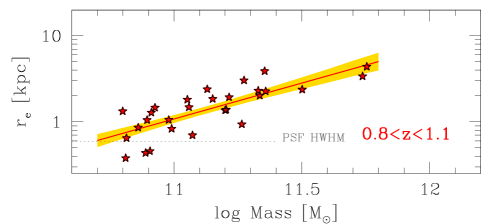
Figure 2: Mass-size relation of red-sequence early-type galaxies at $z>0.8$. Sizes are corrected for PSF blurring effects. The red solid line and yellow shading show the fitted mass-size relation and its 68 % uncertainty (posterior highest density interval). The horizontal dotted line indicates the PSF half width at half maximum (HWHM).

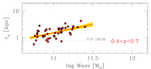
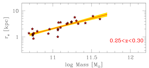
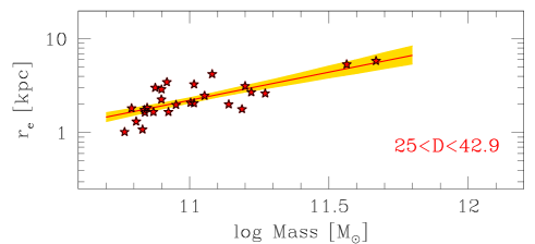
Figure 3: Mass-size relation of red-sequence early-type galaxies at $z<0.7$. Sizes are corrected for PSF blurring effects, although the correction is negligible. The red solid line and yellow shading show the fitted mass-size relation and its 68 % uncertainty (posterior highest density interval). The horizontal dotted line indicates the PSF HWHM (in the middle and bottom panels it is smaller than the displayed range).

The PSF smears images and therefore makes galaxies appear larger than they actually are. We correct for PSF blurring by computing, following Saglia et al. (1993), the size correction as a function of the observed half-light radius expressed in FWHM units and assuming an $r^{1/4}$ radial profile. We applied the correction on a galaxy-by-galaxy basis, and we list the applied correction in Table 1. The correction is, in practice, zero at $z<1$, and then increases at higher redshifts mostly because of the broader PSF in NIR. The correction is important only at $z>1.4$ because of the reduced galaxy sizes there and the larger PSF. For cluster galaxies at the same redshift and band (Paper I), the correction turned out to be negligible because of the larger galaxy sizes in richer environments.

4 Results

Table 1 lists coordinates, mass, and size (half-light radius) of the 170 early-type galaxies on the red sequence studied in this work. Fig. 2 and 3 show the mass-size relation of early-type galaxies on the red sequence at the various redshifts. Identical plots are presented in Paper I for cluster members.

4.1 Checks

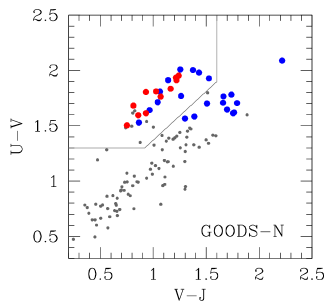
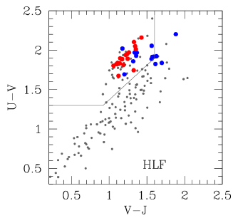
Figure 4: $U-V$ vs $V-J$ diagram of the galaxies with $H$ mag brighter than a SSP with $\log M/M_{\odot}=10.7$ and $z_{f}=3$, with good photometry (use_phot=1), $1.4<z<2.0$ in GOODS-N (left panel) or $1.1<z<1.4$ in HLF (right panel). Red/blue points are early-/late-type red-sequence galaxies with $H$-band derived masses higher than 10.7. The gray solid line separates quiescent and star-forming galaxies according to Williams et al. (2009).

4.1.1 Sample classification

We classify galaxies following the definitions of the morphological types. Other works do not apply this morphological selection or adopt different definitions for the morphological types leading in the case of clusters to samples 30% to 50% contaminated by non-early-type galaxies, as detailed in Appendix C of Paper I. More in general, UVJ quiescent galaxies are easily 30% contaminated by dusty star-forming galaxies (Williams et al. 2009; Moresco et al. 2013). For the current field sample, we found that red-sequence early-type galaxies are all UVJ quiescent galaxies (see Fig. 4; UVJ photometry and classification is from Skelton et al. 2014), that red-sequence galaxies only compose two thirds of UVJ quiescent sample (see Fig. 5) and that only about half of them are morphologically early-type galaxies (see Fig. 5 and 6) in line with our previous works on cluster galaxies (Andreon 1997; Paper I). Therefore, red-sequence early-type galaxies compose just one-third of the UVJ quiescent population. Figure 6 shows some illustrative examples of red-sequence UVJ quiescent galaxies yet morphological late-type. The latter galaxies have a morphological appearance showing that they are forming stars, or have just stopped forming them, in spite of being called quiescent by UVJ colors and being on the red sequence. To summarize, UVJ quiescent galaxies are a broader population than red-sequence morphologically early-type galaxies and the quiescent class includes newcomers: one-third of them are yet not red enough to be on the red sequence, and half of the remaining are not yet morphologically early.

Galaxy populations selected with different criteria may well evolve differently (e.g., Carollo et al. 2013; Andreon et al. 2016). Combining or comparing samples selected in different ways is prone to systematics and must be avoided. We use consistent identical selection in color and morphology across environments and epochs.

4.1.2 Half-size radius

The half-light radius is the radius that encloses half of the galaxy luminosity and our analysis strictly adopts this definition. Many other works adopt a different definition of galaxy size, coincident with the half-light radius for ideal galaxies rare in the real Universe (galaxies with a perfect Sersic profile and without bulge, bar, disk, arms, position angle twists, and without radial changes in the ellipticity). As discussed in Appendix B of Paper I, these scale lengths should be combined with, or compared to, our half-light radii with great caution. At the light of the frequent presence in real galaxies of isophote twists making a curved major axis, the advantages of major axis radii over circularized radii, proposed in some past works, should be reconsidered when, as usual, major axis profiles are derived along a single straight line that ignores the major axis curvature.

Restricting the attention to red-sequence morphologically early-type galaxies only and for which half-light radius and scale lengths are measured in the same photometric band (for which a rough agreement is expected), we found $<0.1$ dex systematics with circularized scale radii in van der Wel et al. (2014), and 0.0 dex with those in van der Wel (2012). For galaxies in our immediate neighborhood, our measurements agree with the values originally measured by Cappellari et al. (2013) and disagree with the values listed in their table because the latter are scaled up by $1.35$. We also have galaxies in common with Cassata et al. (2011), who use a redder band, however. They measured 0.07 dex smaller effective radii consistent with expected color gradients of early-type galaxies.

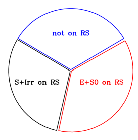
Figure 5: Partitioning of UVJ quiescent galaxies in galaxies not on the red-sequence (RS), RS galaxies of early-type morphology (E+S0), and RS galaxies of late-type morphology (S+Irr).

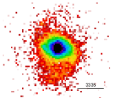
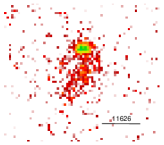
Figure 6: Remarkable cases of UVJ quiescent galaxies on the red sequence yet of late morphological type. These galaxies have manifestly irregular or S-shaped isophotes. The tick is 1 arcsec. The numbers are the IDs in 3DHST paper.

4.1.3 Mass

Our mass estimate, similar to those obtained from fitting photometric data (e.g., Skelton et al. 2014, Laigle et al. 2016) comes from a total flux measurement (at $\lambda\sim 6000$ Å in our case) and a determination of the galaxy age (providing the $M/L$). Our total magnitudes agree well with the total magnitudes of van der Wel et al. (2014) and van der Wel (2012) for common galaxies. The adopted spectral energy distribution template (a simple stellar population with $z_{f}=3$, see Sec. 3) matches the observed color of the red sequence and therefore it is not expected to be grossly in error about the $M/L$.

However, after conversion to a common initial mass function, we agree with the masses in Skelton et al. (2014) at high redshift, but we increasingly disagree with decreasing redshift, up to 0.28 dex at $0.4<z<0.7$. We found this to be due to different assumptions about the galaxy ages: we adopted an old age ($z_{f}=3$), while our red-sequence early-type galaxies typically have a star formation time onset (usually called age) of 2 Gyr independent of redshift according to the values tabulated in Skelton et al. (2014) and adopted by these authors to estimate masses. While at high redshift a 2 Gyr age roughly corresponds to our assumed age, at intermediate redshifts an age of 2 Gyr seems implausible low (e.g., Thomas et al. 2005; Gallazzi et al. 2014). For example, massive galaxies (with no color or morphological pre-selection) at $z=0.7$ have spectroscopic ages of 4.4 Gyrs (Gallazzi et al. 2014), while the typical age derived by template fitting of photometric data by Skelton et al. (2016) is 2 Gyr for the reddest objects (and less for bluer ones). Since galaxies are younger in Skelton et al. (2016) than we assume (and increasingly so with decreasing redshift), their mass is lower for the same luminosity (and increasingly so with decreasing redshift), which explains the increasing discrepancy with decreasing redshift. When our assumed age and that estimated in Skelton et al. (2016) are similar (at high redshift), masses turn out to agree.

At $0.25<z<0.4$ our masses are larger by 0.17 dex than those Laigle et al. (2016) estimate (from photometry) because the typical age of our red-sequence early-type galaxies is 5.5 Gyr in Laigle et al. (2016) versus our adopted age of 8 Gyr.

Therefore, the adopted age has an important impact on the measured size at a given mass and on its evolution: a 0.3 dex discrepancy in mass measured at $z\sim 0.6$ (and none at $z\gtrsim 1.2$) with the Skelton et al. (2014) values, and a size-mass slope of about 0.6 imply a systematic difference of 0.18 dex in sizes (at low z only). This is larger than the error on the mean size of a $\log M/M_{\odot}=11$ and comparable in absolute value to the variation we found in Sec. 4.2 between these redshifts. Therefore, the correctness of the derived size growths depends upon the accuracy of the assumed/derived galaxy age.

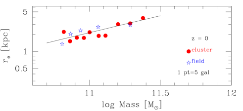
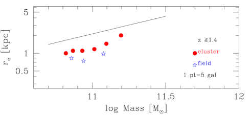
Figure 7: Qualitative comparison of the mass-size distribution of $10.8<\log M/M_{\odot}<11.7$ red-sequence early-type galaxies at low (top panel) and high (bottom panel) redshift. Each point is the average of five galaxies. The solid line indicates the scaling at $z=0$, and it is also shown in the bottom panel to show the evolution more clearly.

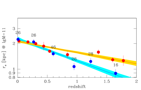
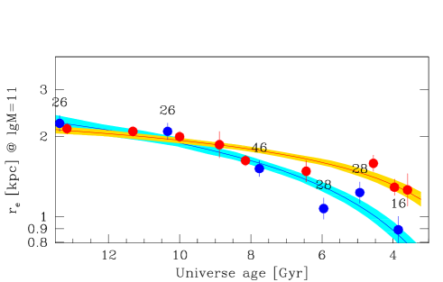
Figure 8: Halo effect on galaxy size and its dependence on look-back time. The figure shows the mean galaxy size at $\log M/M_{\odot}=11$ vs redshift (left panel) or look-back time (right panel) for red-sequence early-type galaxies in the field (blue points) and in cluster (red points). The number above the blue points indicates the number of combined galaxies. The solid line and shading show the fitted relation and its 68 % uncertainty (posterior highest density interval).

Table 2: Mass-size fitting parameters: intercept $\gamma$, slope $\alpha$, and intrinsic scatter $\sigma$ for the various samples

Sample	$\gamma$	$\alpha$	$\sigma$	$N_{gal}$
$1.4<z<2.0$	$-0.05\pm 0.05$	$0.59\pm 0.37$	$0.21\pm 0.04$	$16$
$1.1<z<1.4$	$0.09\pm 0.04$	$0.50\pm 0.26$	$0.20\pm 0.03$	$28$
$0.8<z<1.1$	$0.03\pm 0.04$	$0.83\pm 0.14$	$0.19\pm 0.02$	$28$
$0.4<z<0.7$	$0.18\pm 0.03$	$0.65\pm 0.15$	$0.17\pm 0.02$	$46$
$0.25<z<0.30$	$0.32\pm 0.03$	$0.78\pm 0.11$	$0.14\pm 0.02$	$26$
$25<D<42.9$	$0.35\pm 0.03$	$0.60\pm 0.12$	$0.14\pm 0.02$	$26$

4.2 Trends

Qualitatively, the key result of this work is qualitatively illustrated in Fig. 7 using a portion of the data only, where each point is the average of five galaxies in order to emphasize the mean relation and downweight the scatter around it. The top panel shows that mass-size relations of the Coma cluster and of the local field are very close to each other, while galaxies at higher redshift (bottom panel) are smaller, and those in sparse environments tend to be smaller than their counterparts in clusters. In the following, we put on solid ground this qualitative trend using the whole dataset.

Half-light radii and masses in each redshift bin are fitted using a linear model with intrinsic scatter $\sigma$ of the form

$$\log r_{e}=\gamma\ +\alpha(\log M/M_{\odot}-11)+\mathcal{N}(0,\sigma^{2})$$ (1)

adopting uniform priors for all parameters except the slope $\alpha$, for which we took instead a uniform prior on the angle $b=\arctan\alpha$. The parameter $\gamma$ is, by definition, the average size at $\log M/M_{\odot}=11$. Our approach improves upon past works in two respects. First, the information content of each individual point has a minimal floor given by the large scatter around the mass-size relation (the scatter $\sigma$), while many past analyses (included all stacking ones) account only for the smaller radius measurement error. Second, by leaving the slope free we also allow different evolutions for galaxies of different mass, discarded a priori by the works that keep the slope fixed (e.g., Carollo et al. 2013, or Yano et al. 2016). The free slope also de-weights galaxies with fairly different masses, allowing us to focus on $\log M/M_{\odot}=11$ galaxies.

Fig. 2 and 3 show the fitted trends and their uncertainty. Fit parameters are listed in Table 2. Slope and intrinsic scatter are consistent across redshifts, but by leaving them free we do not overly constrain the fit negating a priori mass-dependent evolutions and differences in scatter.

Fig. 8 shows the effective radius at $\log M/M_{\odot}=11$ (i.e., $\gamma$) as a function of redshift. We fitted them with a linear relation in $z$,

$$\gamma_{z}=\gamma_{11,z=0.6}\ +\beta(z-0.6)$$ (2)

adopting uniform priors for the intercept at $z=0.6$, $\gamma_{11,z=0.6}$, and a uniform prior on the angle $a=\arctan\beta$. In other terms, we are fitting the effective radius at $\log M/M_{\odot}=11$ against $(z-0.6)^{\beta}$.

The mean size of red-sequence early-type galaxies in the field has grown by $0.26$ dex per unit redshift in the last 10 Gyr (at fixed mass), see Table 3. Since the growth is nearly linear in redshift and the relation between redshift and look-back time is bent, this results in an accelerated evolution at earlier epochs (Fig. 8, right panel) in agreement with previous works, for example with Newman et al. (2012, we found an identical value of the slope $\beta$) based, however, on a broader class of galaxies (UVJ selected, see Sec. 4.1.1) and on scale lengths (see Sec. 4.1.2).

Fig. 8 also shows the effective radius at $\log M/M_{\odot}=11$ (i.e., $\gamma$) for cluster galaxies (from Paper I), identically selected and analyzed. Fitting the cluster data with eq. 2 gives an evolutionary rate that is twice lower than for identically selected and analyzed field galaxies, see Table 3, indicating that at $z<2$ the growth is twice as slow in clusters than it is in sparse environments. The larger size at $z>1.5$ of cluster galaxies implies that growth was accelerated at a redshift outside the studied redshift, i.e., at $z>2$. Both fits are acceptable (at better than 90% confidence level) in a $\chi^{2}$ sense, as can also be appreciated by detailed inspection of Fig. 8.

Table 3: Size evolution fitting parameters: intercept at $z=0.6$ and $\log M/M_{\odot}=11$, $\gamma_{11,z=0.6}$, and evolutionary term $\beta$

Sample	$\gamma_{11,z=0.6}$	$\beta$
field	$0.20\pm 0.01$	$-0.26\pm 0.03$
cluster	$0.25\pm 0.01$	$-0.13\pm 0.02$

As mentioned in the introduction, galaxies in massive halos are expected to experience accelerated size growth compared to galaxies in sparser environments, although theory is unable to provide a robust quantitative prediction. For example, the Illustris simulations does not fit the $z=0$ mass-size scaling (Nelson et al. 2015), and the successor IllustrisTNG simulation output galaxies whose size is half the earlier simulation (Pillepich et al. 2018), and does not offer predictions for galaxies of different morphological classes or in different environments, nor does it predict the epoch-dependent growth, hence effectively precluding comparisons. Semi-analytic models do not reproduce this expected behavior (see Sec. 5.2). The quality of our data and the wide redshift sampling allow us to quantify the qualitative expectation and establish the halo effect, and also to determine the dependence of the amplitude on look-back time, as determined above.

The epoch at which red-sequence early-type galaxies in sparse environments catch up with their cousins in richer environments can be easily inferred (the intersection of the two fits in Fig. 8), it is just matter of performing a joint fit of both cluster and field data with a unique intercept for the two datasets at the crossing redshift $z_{catchup}$. By taking a uniform distribution as prior of $z_{catchup}$, zeroed for unphysical values of redshift, and a uniform prior on the angles, the joint fit of both cluster and field data gives $z_{catchup}=0.25\pm 0.13$. The delayed growth of galaxies in sparse environments, combined with their fast growth at $z<2$, makes galaxies of the same size around $z_{catchup}=0.25\pm 0.13$.

Our data allow us to establish whether galaxies in different environments have similar or different sizes, and the approximate time when their sizes match. To further improve the localization of the catch-up redshift, a dataset that more densely samples the low-redshift Universe is needed and, furthermore, a redshift-unbinned analysis is preferable (and easy to implement, for example as in Andreon 2012).

Fig. 9 shows that the scatter around the mass-size relation, $0.15-0.20$ dex (Table 2, see Paper I for cluster values) is fairly constant with environment and epoch, with some possible indication of a larger value in the field. The scatter measures the variability from galaxy to galaxy of the amount of dissipation, integrated over cosmic time, in the system that will form the observed galaxy. Its non-zero value indicates that there is some variation from galaxy to galaxy. The little or no evolution seen in both field and cluster environments and the little or no difference between their amplitudes in the two environments indicates that the amount of dissipation of the system that formed the observed galaxy does not vary greatly with epoch or environment.

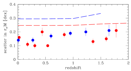
Figure 9: Scatter around the mass-size relation vs redshift. Red points are cluster measurements, blue points field measurements, and red/blue dashed curves are model predictions for cluster/field.

5 Discussion

5.1 Comparison with other determinations

When comparing our results with the results from other works, it should be remembered that red-sequence early-type galaxies only are one-third of quiescent galaxies frequently studied in the literature, and the broader class may evolve differently from each part, as already pointed out. Our red-sequence early-type galaxies form a more homogeneous and narrower class than quiescent or Sersic-index selected samples. In addition, our derivation of the half-light radius accounts for the common features of early-type galaxies, while many works adopt scale lengths susceptible to the presence of galaxy morphological features.

Generally speaking, when compared to other works our analysis benefits from a larger redshift and environmental baselines, allowing us to sample the epoch where environmental effects are more manifest and at the same time, the epoch when such differences are less obvious. The larger redshift baseline allows us to study the epoch-dependence of environmental effects, precluded to previous works.

For example, compared with the high-redshift work by Lani et al. (2013), our sample probes much wider redshift and environmental ranges, benefits from spectroscopic redshifts (i.e., is free of photo-z catastrophic outliers), has the advantage of images that have three times higher resolution (check in Fig. 2 the kpc scale for such degraded resolution), splits the galaxy population into classes that are more homogeneous (their UVJ passive sample includes old early-type galaxies, and galaxies still star-forming or just quenched, based on morphology, see Figs. 4 and 5), and size derivation allows galaxies to be multi-component. The larger redshift baseline allows us to study the epoch-dependence of environmental effects, precluded by their sample.

Compared with Cooper et al. (2012), the studied sample offers much wider redshift and environmental ranges, more bands for size determination to minimize systematics due to color gradients (we used three filters instead of one over the common redshift range), and galaxy populations are split into more homogeneous classes. The larger redshift baseline allows us to study the epoch-dependence of environmental effects, precluded by their sample. As found by Delaye et al. (2014), we found larger galaxies in clusters; however our sample probes a much larger redshift range (their clusters are at $0.84<z<1.45$) allowing us to sample the catch-up redshift (not sampled by them). We also uses a homogeneous sampling of rest-frame wavelength for radii determination (they noted that wavelength differences between cluster and field may affect their conclusions, as also remarked by Saracco et al. 2017). Furthermore, galaxy populations are split into more homogeneous classes, and size derivation allows galaxies to be multi-component.

Generally speaking, our results allow us to understand the variance in the literature results if they are applicable to scale lengths and to the larger class of quiescent galaxies. For example, Huertas-Company et al. (2013) find no environmental dependence, but they studied $z<1$ only, a redshift range where differences are small (see Fig. 6), and even more so given the restricted range of environments in their sample (they lack rich clusters). Similarly, at $0.4<z<0.8$, Kelkar et al. (2015) and, at $0.2<z<0.7$, Morishita et al. (2017) found no environmental difference because they focused on an epoch when environment and halo mass show a small difference at most. At $0.1<z<0.15$, Yoon et al. (2017) found no environmental effects for $\log M/M_{\odot}\approx 11$ galaxies, in agreement with our results, but their studied redshift range is too small to yield the redshift-dependence we detect and their study focuses on an epoch when environmental differences are minor.

Instead, Saracco et al. (2017) found no environmental difference between the sizes of cluster and field elliptical galaxies at $z\sim 1.3$, while we found one for ellipticals and lenticulars. However, apart from differences in morphological composition (we include all lenticulars, while Saracco et al. (2017) only include those difficult to distinguish from ellipticals, such as non-edge-on lenticulars), their galaxy selection differs between cluster and field because galaxies are color (red-sequence) selected for the cluster sample, while galaxies of all colors are considered for the field. We instead performed the same color selection in both cluster and field. Bluer quiescent galaxies tend to be larger than redder ones (e.g., Carollo et al. 2013; Belli et al. 2015), and indeed young early-type galaxies are larger than old ones (Saracco et al. 2009). When blue early-type galaxies are included exclusively in the field sample, they increase the mean size in this environment, hence reducing the difference between cluster and field. Finally, two of three of their field samples have measurements (band used for size determination) or selections (morphological classification and redshift range) differing from the cluster sample.

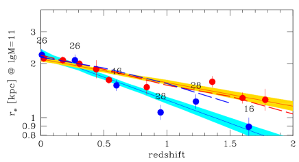
Figure 10: As the left panel of Figure 8, with superposed predictions (dashed curves) for galaxies in $\log M>14.3$ halos (red) and in $\log M<13.3$ halos (blue).

5.2 Comparison with semi-analytic models

Fig. 10 compares the observed half-light size of $\log M/M_{\odot}=11$ early-type galaxies on the red sequence at various redshifts (points and solid lines) with predictions by the semi-analytic model in Shankar et al. (2013) for $10.8<\log M<11.2$ satellites in massive halos (with $\log M>14.3$, red dashed line hardly distinguishable from our fit to data) and for central galaxies of low-mass halos (with $\log M<13.3$, blue dashed line). In simulations (and in observations too), satellites are both galaxies having lost their sub-halo and those still having it but embedded in a larger halo (type 1 and 2 in the code used by Shankar et al. 2013). To better compare with observations, simulations assume random statistical uncertainties in effective radius, stellar mass, and halo mass of 0.08 dex, 0.1 dex, and 0.1 dex, respectively. The Shankar et al. (2013) model adopts the Guo et al. (2011) semi-analytic model inclusive of gas dissipation in major gas-rich mergers and null orbital energies (parabolic orbits). In simulations galaxies are selected at the redshift $z$ to have a bulge-to-total ratio higher than to 0.5 to mimic our morphological selection, and a specific star formation rate lower than $10^{-11}$ M_⊙/yr to mimic our observational red-sequence selection (although the precise value of the threshold has virtually no impact on model predictions). Since for observations we measure projected half-light radii, three-dimensional effective radii in semi-analytic models are projected assuming a de Vaucouleurs profile, as in Shankar et al. (2013). With the above choices, models predict a $(1+z)^{\sim 0.5}$ evolution in both environments (Fig. 10).

The agreement between model predictions and observations is impressive for galaxies in massive halos at all redshifts (compare the solid and dashed red curves) and even more so considering that model sizes have not been re-normalized, unlike the comparison in Huertas-Company et al. (2013). Once considering the lack of re-normalization, the agreement is also remarkable at $z\lesssim 0.5$ in sparse environments. In these sparse environments, the evolution seen in the data over the whole redshift range is closer to $(1+z)^{\sim 1}$ than to $(1+z)^{\sim 0.5}$ predicted by the model. The original model by Guo et al. (2011) predicts similar trends in size evolution (F. Shankar, private communication). Data support a delayed and faster size growth in low-mass halos compared to semi-analytic predictions: delayed because at $z\sim 1$ simulations overpredict galaxy sizes in the field and faster because the observed size growth proceeds at a faster rate (at $z<2$) in the data than in the model for field galaxies. For cluster galaxies, the model growth rate is appropriate to $z\lesssim 2$ and any additional delay, if any, should be minimal and fit in the short time available at $z>2$ in order not to destroy the agreement between model and data observed at $z<2$.

Fig. 9 compares the observed and predicted scatters around the mass-size relation at various redshifts and for the two environments (cluster/field are in red/blue, points are observed values, model predictions are dashed lines). We note that the scatter in size induced by the scatter between true and estimated stellar mass and by size errors are consistently left inside the derived scatter in size at a given mass, i.e., in the plotted points and curves. The smallest and most precise observed scatter is about 0.1 dex, equal to the expected combined effects of size and stellar mass errors (the latter assumed for the model predictions). The model predicts a close to constant scatter, as already pointed out in Shankar et al. (2013) and as seen in the data, as welle as a larger scatter in the field environment, as the data may also indicate. However, the model systematically overpredicts the observed scatter (as already noted at redshift zero by Shankar et al. 2013), possibly indicating an overestimation of the amount of dissipation implemented in the model. We warn however that different methodologies are used to measure the scatter for the real data and the semi-analytic data.

5.3 Are environment effects on size growth epoch dependent?

The continuity seen in the size growth in both environments (Fig. 8) suggests that the environment keeps its effects constant and continues to increase galaxy sizes at different rates in different environments and that the environment never stops having an effect on the galaxy sizes. The observed similarity of sizes in different environments at low to intermediate redshift is due to this epoch corresponding to the catch-up epoch, not to the cessation of the environment effects. The data seem to suggest that there is no transition epoch below which the environment stops affecting sizes (i.e., where the derivative of trend with redshift becomes zero), but a catch-up epoch at which the faster growth of galaxies in sparser environments makes them reach the size of their cousins in more massive environments. As mentioned, because of the non-linear relation between redshift and look-back time, a rate constant per unit redshift is instead varying per unit time (Fig. 8).

We note that in the literature environmental effects are investigated comparing the effective radius (at a given mass) in different environments at a single redshift (or a small range). While useful, this choice is subject to degeneracies because the observed size is the result of environmental effects integrated over time and there may well be two different functions with identical integrals. For example, environment may play a major role, but at different times back in the galaxy history, hard to guess from a sample of equal-sized galaxies in all environments at low or intermediate redshifts: is their similarity the result of an environmental-independent growth, or of two widely different growth histories having the same integral? The richness of our sample, and in particular the wide sampling in epoch allowing us to measure the derivative of the galaxy size, breaks the degeneracy of measurements at a fixed redshift and allow to determine the environmental dependence, and its epoch dependence, of the galaxy growth.

6 Conclusions

We carried out a photometric and structural analysis in the rest-frame $V$ band of a mass-selected ($\log M/M_{\odot}>10.7$) sample of red-sequence early-type galaxies with spectroscopic/grism redshift in the general field up to $z=2$. The sample is composed of 170 red-sequence early-type galaxies in the general field and complements the sample of 224 early-type galaxies in clusters identically observed and analyzed (presented in Paper I). The two samples are in environments differing by 3 orders of magnitude in density and 2 orders of magnitude in halo mass.

Because of the morphology and the narrower color selection of the sample addressed in our study, red-sequence early-type galaxies are one-third only of the larger quiescent galaxy population, the latter including bluer galaxies and morphological late-type galaxies with evolutionary paths different from the remaining part of the quiescent population. The tighter selections helps to disentangle the evolution of the population from different levels of contaminations in different environments or at different epochs, i.e., between galaxy properties and sample selection.

We homogeneously, both across redshifts and environments, derived sizes (effective radii) fully accounting for the multi-component nature of galaxies and the common presence of isophote twists and ellipticity gradients, allowing us to determine the epoch dependence of environmental effects. Comparison with masses in the literature for common galaxies put forth the important consequences on the inferred size evolution of systematics to mass determination, such as the adopted age of the stellar population.

Observationally, red-sequence early-type galaxies in the field are smaller at high redshifts compared to descendants and to objects at the same redshift in clusters, and their size growth rate is about twice as large as than for objects in the cluster environments ($0.26\pm 0.03$ versus $0.13\pm 0.02$ dex per unit redshift) so that objects in the field reached the dimension of those in cluster at $z=0.15\pm 0.12$. Environment affects early-type galaxy sizes in an epoch-independent way at $z<2$ when the size growth rate is measured per unit redshift. In particular, there is no $z<2$ epoch when environment stops affecting galaxy sizes. Data point toward a model where size growth is epoch-independent (i.e., $\partial\log r_{e}/\partial z=c$) but with a rate $c$ depending on environment, $\partial c/\partial\log M_{halo}\approx 0.05(=(0.26-0.13)/2.5)$, where $2.5$ is the mass difference, on log scale, between field and cluster halos (Sect. 1).

Early-type galaxies are larger in massive halos at high redshift indicating that their size build up earlier (at $z>2$) at an accelerated rate, slowing down at some still unidentified $z>2$ redshift. Instead, the size growth rate of red-sequence early-type galaxies in low-mass halos is reversed: it proceeds at an increased rate at late epochs after an early period ($z>2$) of reduced growth, in agreement with the qualitative hierarchical picture of galaxy evolution. Semi-analytical models considered in this work get close to the observed behavior, but predicts a too fast early growth and a too mild late evolution for galaxies in the field.

The scatter around the mass-size relation, $0.15-0.20$ dex, is fairly constant with environment and epoch and measure the variety from galaxy to galaxy of the amount of dissipation integrated over cosmic time of the initial energy of the system that formed the observed galaxy. The little or no evolution seen in both field and cluster samples and the little or no difference between their amplitude in the two environments indicates that the amount of dissipation does not vary greatly with epoch or environment.

Appendix A Sample composition, completeness and contamination

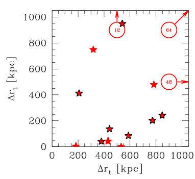
Figure 11: Trasverse and longitudinal comoving distance from the nearest galaxy in the sample. Symbols with black boundaries refer to GOODS-N, those entirely red are galaxies in HLF. No galaxy in the COSMOS field falls in the shown part of the plot. Circles with arrows indicate the number of galaxies outside the plot. Galaxies in our immediate neighborhood are not considered in this plot.

In general, random exclusion of galaxies from a sample does not bias the sample and results based on it (although they do reduce the sample power). Incompleteness instead biases results when galaxies are removed with preference (when their size is larger/smaller than average for their mass, in the case of our work). Contamination may also bias results if unwanted galaxies have properties different from those wanted (e.g., larger/smaller or more heterogeneous, at a fixed mass, in the case of our work). Finally, differences in distribution in mass of the studied sample do not bias results at a fixed mass, but can reduce the statistical power of the sample. For example, adding $\log M/M_{\odot}>11.9$ galaxies to a sample of $\log M/M_{\odot}\sim 11$ galaxies does not change the average size of $\log M/M_{\odot}\sim 11$ galaxies.

Our work is basically unbiased, but can suffer some limitations. In our work some galaxies are randomly excluded from the sample for various reasons, namely: a) very bright galaxies in the ATLAS3D are over-represented compared to the other samples, especially those at high redshift. For this reason, we discarded all $\log M/M_{\odot}>11.9$ galaxies and only consider a random sample among those immediately less massive. These excluded galaxies have a much higher mass than those of interest and therefore including or removing them does not changes the size of lighter galaxies that are the focus of our work. Furthermore, we did not select against galaxies larger (or smaller) than average for their mass, we simply skip the analysis of bright ATLAS3D galaxies after having collected some of them in the sample; b) target galaxies falling in unfortunate locations of images, including on the boundaries, on a sharp gradient in exposure time, on a satellite track, on the top of a diffraction spike, or close to bright star or an unrelated galaxy. As mentioned, since the reason for exclusion is independent of the target galaxy (size at a given mass), exclusion is random and our results are not biased by the removal of these galaxies.

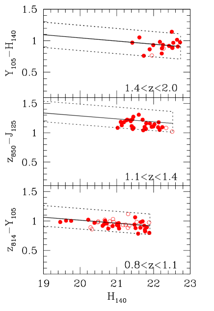
Figure 12: Color–magnitude plot of red-sequence early-type galaxies for galaxies at $z<0.8$. The slanted rectangles indicate the selection region. Close points are analyzed galaxies, open points indicate galaxies with unfeasible isophotal analysis.

About sample contamination, since we only want central galaxies, we removed from the sample all satellite galaxies in groups. This operation was fairly straightforward because of the isolation of most of the galaxies and the quality of the used data: Fig. A.1 shows the transversal and longitudinal comoving distance of the galaxies left in the sample from the nearest galaxy in the sample after removing obvious satellites plus a few galaxies with unfeasible isophotal analysis (see below). Groups with $M_{500}\approx 10^{12}M_{\odot}$ have $r_{500}=100$ kpc (at $z\sim 1$, to be precise), and no galaxy pair is that close in our sample. Even considering an unrealistic distance four times bigger (in each direction, corresponding to an $M_{500}\sim 6\ 10^{13}M_{\odot}$ rich group or small cluster, hard to miss in these images that are among the deepest ever taken), in our sample there is one contaminating galaxy only. Therefore, even in the unrealistic scenario, our sample is at most contaminated by one galaxy, a $<1$% contamination.

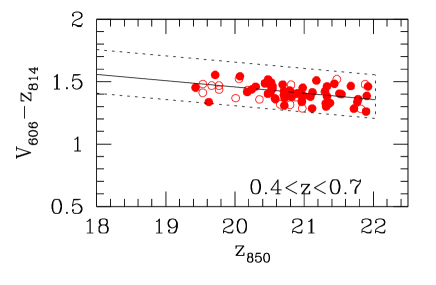
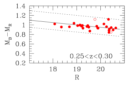
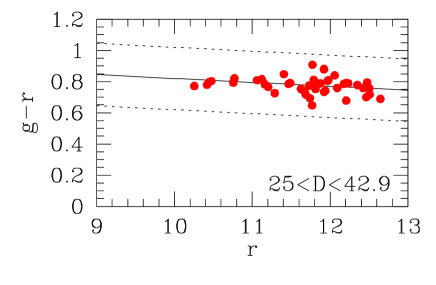
Figure 13: Color–magnitude plot of red-sequence early-type galaxies for galaxies at $z>0.8$. The slanted rectangles indicate the selection region. Full Circles are analyzed galaxies, open circles indicate galaxies with unfeasible isophotal analysis, and/or member of a group or, in the bottom panel only, the sample randomly not selected for the isophotal analysis.

We have two types of sample incompleteness. The first is related to the removal of central galaxies in rich groups, operated to widen the environmental range of our study and often as a matter of necessity since these galaxies are often blended with their satellite and therefore the isophotal analysis is unfeasible anyway. Since the removal is performed by visual inspection, it is ambigous to some extent. These galaxies are often very bright and therefore carry almost no information on the size of $\log M/M_{\odot}\sim 11$ galaxies; including or excluding them from the sample is irrelevant for the quantity of our interest (and non dependently on whether these galaxies should be in principle removed or kept). Second, in a few cases isophote shapes or the galaxy environment turned out to be too complex for our isophotal analysis to succeed. For example, our software is unable to deal with isophote shapes that are not simply connected (i.e., with holes, such as for S0 with an important dust lane seen edge-on at high resolution). Our software is not able to deal with a blend by, say, foreground spiral galaxies or multiple faint galaxies on closeby lines of sight (if feasible at all). The subsample of these galaxies having $\log M/M_{\odot}\sim 11$ is the main source of incompleteness of our sample. To bias our results, this subsample of missing galaxies should consist preferentially of galaxies larger (or smaller) for their mass. Fig. A.1 and A.2 show all studied galaxies (full circles) and the missed galaxies (open circles). Only 15 % of $\log M/M_{\odot}\sim 11$ galaxies do not have a radius determination, and since the reason for exclusion is almost independent on the target galaxy (we would have likely missed most of the galaxies if they were slightly larger or smaller), exclusion is random (“ignorable” is the appropriate statistical term, see the Gelman et al. 2004 book) and our results are not biased by the removal of these few galaxies.