Constraint-based Causal Discovery for Non-Linear Structural Causal Models with Cycles and Latent Confounders

Abstract

We address the problem of causal discovery from data, making use of the recently proposed causal modeling framework of modular structural causal models (mSCM) to handle cycles, latent confounders and non-linearities. We introduce $\sigma$-connection graphs ($\sigma$-CG), a new class of mixed graphs (containing undirected, bidirected and directed edges) with additional structure, and extend the concept of $\sigma$-separation, the appropriate generalization of the well-known notion of d-separation in this setting, to apply to $\sigma$-CGs. We prove the closedness of $\sigma$-separation under marginalisation and conditioning and exploit this to implement a test of $\sigma$-separation on a $\sigma$-CG. This then leads us to the first causal discovery algorithm that can handle non-linear functional relations, latent confounders, cyclic causal relationships, and data from different (stochastic) perfect interventions. As a proof of concept, we show on synthetic data how well the algorithm recovers features of the causal graph of modular structural causal models.

1 INTRODUCTION

Correlation does not imply causation. To go beyond spurious probabilistic associations and infer the asymmetric causal relations we need sufficiently powerful models. Structural causal models (SCMs), also known as structural equation models (SEMs), provide a popular modeling framework (see [32, 25, 26, 12]) that is up to this task. Still, the problem of causal discovery from data is notoriously hard. Theory and algorithms need to address several challenges like probabilistic settings, stability under interventions, combining observational and interventional data, latent confounders and marginalisation, selection bias and conditioning, faithfulness violations, cyclic causation like feedback loops and pairwise interactions, and non-linear functional relations in order to go beyond artificial simulation settings and become successful on real-world data.

Several algorithms for causal discovery have been introduced over the years. For the acyclic case without latent confounders, numerous constraint-based [25, 32] and score-based approaches [17, 14, 6] exist. More sophisticated constraint-based [25, 32, 5, 34] and score-based approaches [7, 10, 11, 8, 4] can deal with latent confounders in the acyclic case. For the linear cyclic case, most algorithms assume no latent confounders [27, 29, 18], though some of the more recent ones allow for those [19, 30]. To the best of our knowledge, no algorithms have yet been proposed for the general non-linear cyclic case.

In this work we present a novel conditional independence constraint-based causal discovery algorithm that—up to the knowledge of the authors—is the first causal discovery algorithm that addresses most of the previously mentioned problems at once, notably non-linearities, cycles, latent confounders, and multiple interventional data sets, only excluding selection bias and faithfulness violations.

For this to work we build upon the theory of modular structural causal models (mSCM) introduced in [12]. mSCMs form a general and convenient class of structural causal models that can deal with cycles and latent confounders. The measure-theoretically rigorous presentation opens the door for general non-linear measurable functions and any kind of probability distributions (e.g. mixtures of discrete or continuous ones). mSCM are provably closed under any combination of perfect interventions and marginalisations (see [12]).

Unfortunately, it is known that the direct generalization of the d-separation criterion (also called m- or m^∗-separation, see [24, 33, 25, 9, 28]), which relates the conditional independencies of the model to its underlying graphical structure, does not apply in general if the structural equations are non-linear and the graph contains cycles (see [31, 12] or example 2.17).

Luckily, one key property of mSCMs is that the variables of the mSCM always entail the conditional independences implied by $\sigma$-separation, a non-naive generalization of the d/m/m^∗-separation (see [12]), which also works in the presence of cycles, non-linearities and latent confounders, and reduces to d-separation in the acyclic case.

To prove the $\sigma$-separation criterion, the authors of [12] have constructed an extensive theory for directed graphs with hyperedges. As a first contribution in this paper we give a simplified but equivalent definition of mSCMs plainly in terms of directed graphs and prove the $\sigma$-separation criterion directly under weaker assumptions.

As a second contribution we extend the definition of $\sigma$-separation to mixed graphs (including also bi- and undirected edges) by introducing additional structure. We will refer to this class of mixed graphs as $\sigma$-connection graphs ($\sigma$-CG), since they are inspired by the d-connection graphs introduced by [19]. We prove that $\sigma$-CGs and $\sigma$-separation are closed under marginalisation and conditioning, in analogy with the d-connection graphs (d-CG) from [19].

The work of [19] provides an elegant approach to causal discovery using a weighted SAT solver to find the causal graph that is most compatible with (weighted) conditional independences in the data, encoding the notion of d-separation into answer set programming (ASP), a declarative programming language with an expressive syntax for implementing discrete or integer optimization problems. Our third contribution is to adapt the approach of [19] by replacing d-separation by $\sigma$-separation and d-CGs by $\sigma$-CGs. The results mentioned above will then ensure all the needed properties to make the adapted algorithm of [19] applicable to general mSCMs, i.e., to non-linear causal models with cycles and latent confounders, under the additional assumptions of no selection bias and of $\sigma$-faithfulness.

Finally, as a proof of concept, we will show the effectiveness of our proposed algorithm in recovering features of the causal graphs of mSCMs from simulated data.

2 THEORY

2.1 MODULAR STRUCTURAL CAUSAL MODELS

Structural causal or equation models (SCM/SEM) usually start with a set of variables $(X_{v})_{v\in V}$ attached to a graph $G$ that satisfy (or are even defined by) equations of the form:

$$X_{v}=g_{\{v\}}(X_{\mathrm{Pa}^{G}(v)},E_{v}),$$

with a function $g_{\{v\}}$ and noise variable $E_{v}$ attached to each node $v\in V$. Here ${\mathrm{Pa}^{G}(v)}$ denotes the set of (direct causal) parents of $v$. In linear models the functions $g_{\{v\}}$ are linear functions, in acyclic models the nodes of $V$ form an acyclic graph $G$, and under causal sufficiency the variables $E_{v}$ are independent (i.e. “no latent confounders”). The functions $g_{\{v\}}$ are usually interpreted as local causal mechanisms that produce the values of $X_{v}$ from the values of $X_{\mathrm{Pa}^{G}(v)}$ and $E_{v}$. These local mechanisms $g_{\{v\}}$ are—in the causal setting—assumed to be stable even when one intervenes upon some of the variables, i.e. one makes a causal local compatibility assumption. One important observation now is that one can also consider the global mechanism $g$ that maps the values of the latent variables $(E_{v})_{v\in V}$ to the values of the observed variables $(X_{v})_{v\in V}$. The assumption of acyclicity or invertible linearity will then guarantee the global compatibility of all these mechanisms $g_{\{v\}}$ and $g$. However, if we now abstain from assuming acyclicity or linearity, the global compatibility does not follow from the local compatibility anymore (see figure 1). So in a general consistent causal setting this needs to be guaranteed or assumed.

Figure 1: Gear analogy. Left: A cyclic mechanism that is locally compatible but not globally. Center: For acyclic mechanisms local compatibility implies global compatibility. Right: A cyclic mechanism that is locally and globally compatible. This shows that the assumption of global compatibility is needed when cycles are present.

The definition of modular structural causal models (mSCM) and the mentioned list of desirable properties basically follow directly from causal postulates:

Postulate 2.1 (Causal postulates).

The observed world appears as the projection of an extended world such that:

1. All latent and observed variables in this extended world are causally linked by a directed graph.

2. Every subsystem of this extended world can be expressed as the joint effect of its joint direct causes.

3. All these mechanisms are globally compatible.

Special subsystems of interest are the loops of a graph.

Definition 2.2 (Loops).

Let $G=(V,E)$ be a directed graph (with or without cycles).

1. A loop of $G$ is a set of nodes $S\subseteq V$ such that for every two nodes $v_{1},v_{2}\in S$ there are two directed paths $v_{1}\mathrel{\leavevmode\hbox to13.6pt{\vbox to3.85pt{\text{[drawing]}}}}\cdots\mathrel{\leavevmode\hbox to13.4pt{\vbox to0.4pt{\text{[drawing]}}}}v_{2}$ and $v_{2}\mathrel{\leavevmode\hbox to13.4pt{\vbox to0.4pt{\text{[drawing]}}}}\cdots\mathrel{\leavevmode\hbox to13.4pt{\vbox to0.4pt{\text{[drawing]}}}}v_{1}$ in $G$ with all the intermediate nodes also in $S$ (if any). The single element sets $S=\{v\}$ are also considered as loops.

2. The strongly connected component of $v$ in $G$ is defined to be:

   $$\mathrm{Sc}^{G}(v):=\mathrm{Anc}^{G}(v)\cap\mathrm{Desc}^{G}(v),$$

   the set of nodes that are both ancestors and descendants of $v$ (including $v$ itself).

3. Let $\mathcal{L}(G):=\{S\subseteq G\;|\,S\text{ a loop of }G\}$ be the loop set of $G$.

Remark 2.3.

Note that the loop set $\mathcal{L}(G)$ contains all single element loops $\{v\}\in\mathcal{L}(G)$, $v\in V$, as the smallest loops and all strongly connected components $\mathrm{Sc}^{G}(v)\in\mathcal{L}(G)$, $v\in V$, as the largest loops, but also all non-trivial intermediate loops $S$ with $\{v\}\subsetneq S\subsetneq\mathrm{Sc}^{G}(v)$ inside the strongly connected components (if existent). If $G$ is acyclic then $\mathcal{L}(G)$ only consists of the single element loops: $\mathcal{L}(G)=\{\{v\}\,|\,v\in V\}$.

The definition of mSCM is made in such a way that it will automatically incorporate the causal postulates 2.1. In the following, all spaces are meant to be equipped with $\sigma$-algebras, forming standard measurable spaces, and all maps to be measurable.

Definition 2.4 (Modular Structural Causal Model, [12]).

A modular structural causal model (mSCM) by definition consists of:

1. a set of nodes $V^{+}=U\dot{\cup}V$, where elements of $V$ correspond to observed variables and elements of $U$ to latent variables,

2. an observation/latent space $\mathcal{X}_{v}$ for every $v\in V^{+}$, $\mathcal{X}:=\prod_{v\in V^{+}}\mathcal{X}_{v}$,

3. a product probability measure $\mathbb{P}:=\mathbb{P}_{U}=\otimes_{u\in U}\mathbb{P}_{u}$ on the latent space $\prod_{u\in U}\mathcal{X}_{u}$,

4. a directed graph structure $G^{+}=(V^{+},E^{+})$ with the properties:

   1. $V=\mathrm{Ch}^{G^{+}}(U)$,

   2. $\mathrm{Pa}^{G^{+}}(U)=\emptyset$,

   3. $\mathrm{Ch}^{G^{+}}(u_{1})\nsubseteq\mathrm{Ch}^{G^{+}}(u_{2})$ for every two distinct $u_{1},u_{2}\in U$,

   where $\mathrm{Ch}^{G^{+}}$ and $\mathrm{Pa}^{G^{+}}$ stand for children and parents in $G^{+}$, resp.,

5. a system of structural equations $g=(g_{S})_{\begin{subarray}{c}S\in\mathcal{L}(G^{+})\\ S\subseteq V\end{subarray}}$:

   $$g_{S}:\;\prod_{v\in\mathrm{Pa}^{G^{+}}(S)\setminus S}\mathcal{X}_{v}\to\prod_{v\in S}\mathcal{X}_{v},$$

   that satisfy the following global compatibility conditions: For every nested pair of loops $S^{\prime}\subseteq S\subseteq V$ of $G^{+}$ and every element $x_{\mathrm{Pa}^{G^{+}}(S)\cup S}\in\prod_{v\in\mathrm{Pa}^{G^{+}}(S)\cup S}\mathcal{X}_{v}$ we have the implication:

   $$\begin{array}[]{rcrcl}&&g_{S}(x_{\mathrm{Pa}^{G^{+}}(S)\setminus S})&=&x_{S}\\ &\implies&g_{S^{\prime}}(x_{\mathrm{Pa}^{G^{+}}(S^{\prime})\setminus S^{\prime}})&=&x_{S^{\prime}},\end{array}$$

   where $x_{\mathrm{Pa}^{G^{+}}(S^{\prime})\setminus S^{\prime}}$ and $x_{S^{\prime}}$ denote the corresponding components of $x_{\mathrm{Pa}^{G^{+}}(S)\cup S}$.

The mSCM can be summarized by the tuple $M=(G^{+},\mathcal{X},\mathbb{P},g)$.

Figure 2: The graph $G^{+}$ of a modular structural causal model (mSCM). The observed variables $v_{i}\in V$ are in blue and the latent variables $u_{j}\in U$ are in red. We have the four observed strongly connected components: $\{v_{1}\}$, $\{v_{2},v_{3},v_{4},v_{5}\}$, $\{v_{6},v_{7}\}$, $\{v_{8}\}$.

Remark 2.5.

Given the mechanisms attached to the nodes $g_{\{v\}}$ the existence (and compatibility) of the other mechanisms $g_{S}$ for non-trivial loops $S$ can be guaranteed under certain conditions, e.g. trivially in the acyclic case, or if every cycle is contractive (see subsection 4.1), or more generally if the cycles are “uniquely solvable” (see [12, 3]).

We are now going to define the actual random variables $(X_{u})_{u\in V^{+}}$ attached to any mSCM.

Remark 2.6.

Let $M=(G^{+},\mathcal{X},\mathbb{P},g)$ be a mSCM with $G^{+}=(U\dot{\cup}V,E^{+})$.

1. The latent variables $(X_{u})_{u\in U}$ are given by the canonical projections $E_{u}:\;\prod_{u^{\prime}\in U}\mathcal{X}_{u^{\prime}}\to\mathcal{X}_{u}$ and are jointly $\mathbb{P}$-independent (by 1). Sometimes we will write $(E_{u})_{u\in U}$ instead of $(X_{u})_{u\in U}$ to stress their interpretation as error/noise variables.

2. The observed variables $(X_{v})_{v\in V}$ are inductively defined by:

   $$X_{v}:=g_{S,v}\big{(}(X_{w})_{w\in\mathrm{Pa}^{G^{+}}(S)\setminus S}\big{)},$$

   where $S:=\mathrm{Sc}^{G^{+}}(v):=\mathrm{Anc}^{G^{+}}(v)\cap\mathrm{Desc}^{G^{+}}(v)$ and where the second index $v$ refers to the $v$-component of $g_{S}$. Note that the inductive definition is possible because when “aggregating” each of the biggest cycles $\mathrm{Sc}^{G^{+}}(v)$ into one node then only an acyclic graph is left, which can be totally ordered.

3. By the compatibility condition for $g$ we then have that for every $S\in\mathcal{L}(G^{+})$ with $S\subseteq V$ the following equality holds:

   $$X_{S}=g_{S}(X_{\mathrm{Pa}^{G^{+}}(S)\setminus S}),$$

   where we put $X_{A}:=(X_{v})_{v\in A}$ for subsets $A$.

As a consequence of the convenient definition 2.4 all the following desirable constructions (like marginalisations and interventions) are easily seen to be well-defined (for proofs see [12]). Note that already defining these constructions was a key challenge in the theory of causal models in the presence of cycles (see [12, 3], a.o.).

Definition 2.7.

Let $M=(G^{+},\mathcal{X},\mathbb{P},g)$ be a mSCM with $G^{+}=(U\dot{\cup}V,E^{+})$.

1. By plugging the functions $g_{S}$ into each other we can define the marginalised mSCM $M^{\prime}$ w.r.t. a subset $W\subseteq V$. For example, when marginalizing out $W=\{w\}$ we can define (for the non-trivial case $w\in\mathrm{Pa}^{G^{+}}(S)\setminus S$):

   $$\begin{array}[]{l}g_{S^{\prime},v}(x_{\mathrm{Pa}^{G^{\prime}}(S^{\prime})\setminus S^{\prime}}):=\\ g_{S,v}(x_{\mathrm{Pa}^{G^{+}}(S)\setminus(S\cup\{w\})},g_{\{w\}}(x_{\mathrm{Pa}^{G^{+}}(w)\setminus\{w\}})),\end{array}$$

   where $G^{\prime}$ is the marginalised graph of $G^{+}$, $S^{\prime}\subseteq V^{\prime}$ is any loop of $G^{\prime}$ and $S$ the corresponding induced loop in $G^{+}$.

2. For a subset $I\subseteq V$ and a value $x_{I}\in\prod_{v\in I}\mathcal{X}_{v}$ we define the intervened graph $G^{\prime}$ by removing all the edges from parents of $I$ to $I$. We put $X_{u}^{\operatorname{do}(x_{I})}:=X_{u}$ for $u\in U$ and $X_{I}^{\operatorname{do}(x_{I})}:=x_{I}$ and inductively ($S:=\mathrm{Sc}^{G^{\prime}}(v)$):

   $$X_{v}^{\operatorname{do}(x_{I})}:=g_{S,v}(X^{\operatorname{do}(x_{I})}_{\mathrm{Pa}^{G^{\prime}}(S)\setminus S}).$$

   By selecting all functions $g_{S}$ where $S$ is still a loop in the intervened graph $G^{\prime}$ we get the post-interventional mSCM $M^{\prime}$. These constructions give us all interventional distributions, e.g. (cf. [25]):

   $$\mathbb{P}(X_{A}|\operatorname{do}(x_{I}),X_{B}):=\mathbb{P}(X_{A}^{\operatorname{do}(x_{I})}|X_{B}^{\operatorname{do}(x_{I})}).$$

   Instead of fixing $X_{I}^{\operatorname{do}(x_{I})}$ to a value $x_{I}$ we could also specify a distribution $\mathbb{P}_{I}^{\prime}$ for it (“randomization”). In this way we define stochastic interventions $\operatorname{do}(\xi_{I})$ with an independent random variable $\xi_{I}$ taking values in $\mathcal{X}_{I}$ and get a $\mathbb{P}^{\operatorname{do}(I)}$ similarly.

2.2 $\Sigma$-SEPARATION IN MSCMS AND $\Sigma$-CONNECTION GRAPHS

We now introduce $\sigma$-separation as a generalization of d-separation directly on the level of mixed graphs. To make the definition stable under marginalisation and conditioning we need to carry extra structure. The resulting graphs will be called $\sigma$-connection graphs ($\sigma$-CG), where the name is inspired by [19]. An example that shall clarify the difference between d- and $\sigma$-separation is given later in figure 2 and table 1.

Definition 2.8 ($\sigma$-Connection Graphs ($\sigma$-CG)).

A $\sigma$-connection graph ($\sigma$-CG) is a mixed graph $G$ with a set of nodes $V$ and directed ($\mathrel{\leavevmode\hbox to13.4pt{\vbox to0.4pt{\text{[drawing]}}}}$), undirected ($\mathrel{\leavevmode\hbox to13.4pt{\vbox to0.4pt{\text{[drawing]}}}}$) and bidirected ($\mathrel{\leavevmode\hbox to13.4pt{\vbox to0.4pt{\text{[drawing]}}}}$) edges, together with an equivalence relation $\sim_{\sigma}$ on $V$ that has the property that every equivalence class $\sigma(v)$, $v\in V$, is a loop in the underlying directed graph structure: $\sigma(v)\in\mathcal{L}(G)$. Undirected self-loops ($v\mathrel{\leavevmode\hbox to13.4pt{\vbox to0.4pt{\text{[drawing]}}}}v$) are allowed, (bi)-directed self-loops ($v\mathrel{\leavevmode\hbox to13.4pt{\vbox to0.4pt{\text{[drawing]}}}}v$, $v\mathrel{\leavevmode\hbox to13.4pt{\vbox to0.4pt{\text{[drawing]}}}}v$) are not.

In particular, every node is assigned to a unique fixed loop $\sigma(v)$ in $G$ with $v\in\sigma(v)$ and two of such loops $\sigma(v_{1})$, $\sigma(v_{2})$ are either identical or disjoint. The reason for why we need such structure is illustrated in figure 5.

Definition 2.9 ($\sigma$-Open Path in a $\sigma$-CG).

Let $G$ be a $\sigma$-CG with set of nodes $V$ and $Z\subseteq V$ a subset. Consider a path $\pi$ in $G$ with $n\geq 1$ nodes:

$$v_{1}\begin{array}[]{c}\mathrel{\leavevmode\hbox to13.4pt{\vbox to0.4pt{\text{[drawing]}}}}\\[-10.0pt] \mathrel{\leavevmode\hbox to13.4pt{\vbox to0.4pt{\text{[drawing]}}}}\\[-10.0pt] \mathrel{\leavevmode\hbox to13.4pt{\vbox to0.4pt{\text{[drawing]}}}}\\[-10.0pt] \mathrel{\leavevmode\hbox to13.4pt{\vbox to0.4pt{\text{[drawing]}}}}\end{array}\cdots\begin{array}[]{c}\mathrel{\leavevmode\hbox to13.4pt{\vbox to0.4pt{\text{[drawing]}}}}\\[-10.0pt] \mathrel{\leavevmode\hbox to13.4pt{\vbox to0.4pt{\text{[drawing]}}}}\\[-10.0pt] \mathrel{\leavevmode\hbox to13.4pt{\vbox to0.4pt{\text{[drawing]}}}}\\[-10.0pt] \mathrel{\leavevmode\hbox to13.4pt{\vbox to0.4pt{\text{[drawing]}}}}\end{array}v_{n}.$$

The path will be called $Z$-$\sigma$-open if:

1. the endnodes $v_{1},v_{n}\notin Z$, and

2. every triple of adjacent nodes in $\pi$ that is of the form:

   1. collider:

      $$v_{i-1}\begin{array}[]{c}\mathrel{\leavevmode\hbox to13.4pt{\vbox to0.4pt{\text{[drawing]}}}}\\[-10.0pt] \mathrel{\leavevmode\hbox to13.4pt{\vbox to0.4pt{\text{[drawing]}}}}\end{array}v_{i}\begin{array}[]{c}\mathrel{\leavevmode\hbox to13.4pt{\vbox to0.4pt{\text{[drawing]}}}}\\[-10.0pt] \mathrel{\leavevmode\hbox to13.4pt{\vbox to0.4pt{\text{[drawing]}}}}\end{array}v_{i+1},$$

      satisfies $v_{i}\in Z$,

   2. (non-collider) left chain:

      $$v_{i-1}\mathrel{\leavevmode\hbox to13.4pt{\vbox to0.4pt{\text{[drawing]}}}}v_{i}\begin{array}[]{c}\mathrel{\leavevmode\hbox to13.4pt{\vbox to0.4pt{\text{[drawing]}}}}\\[-10.0pt] \mathrel{\leavevmode\hbox to13.4pt{\vbox to0.4pt{\text{[drawing]}}}}\end{array}v_{i+1},$$

      satisfies $v_{i}\notin Z$ or $v_{i}\in Z\cap\sigma(v_{i-1})$,

   3. (non-collider) right chain:

      $$v_{i-1}\begin{array}[]{c}\mathrel{\leavevmode\hbox to13.4pt{\vbox to0.4pt{\text{[drawing]}}}}\\[-10.0pt] \mathrel{\leavevmode\hbox to13.4pt{\vbox to0.4pt{\text{[drawing]}}}}\end{array}v_{i}\mathrel{\leavevmode\hbox to13.4pt{\vbox to0.4pt{\text{[drawing]}}}}v_{i+1},$$

      satisfies $v_{i}\notin Z$ or $v_{i}\in Z\cap\sigma(v_{i+1})$,

   4. (non-collider) fork:

      $$v_{i-1}\mathrel{\leavevmode\hbox to13.4pt{\vbox to0.4pt{\text{[drawing]}}}}v_{i}\mathrel{\leavevmode\hbox to13.4pt{\vbox to0.4pt{\text{[drawing]}}}}v_{i+1},$$

      satisfies $v_{i}\notin Z$ or $v_{i}\in Z\cap\sigma(v_{i-1})\cap\sigma(v_{i+1})$,

   5. (non-collider) with undirected edge:

      $$\begin{array}[]{c}v_{i-1}\begin{array}[]{c}\mathrel{\leavevmode\hbox to13.4pt{\vbox to0.4pt{\text{[drawing]}}}}\end{array}v_{i}\begin{array}[]{c}\mathrel{\leavevmode\hbox to13.4pt{\vbox to0.4pt{\text{[drawing]}}}}\\[-10.0pt] \mathrel{\leavevmode\hbox to13.4pt{\vbox to0.4pt{\text{[drawing]}}}}\\[-10.0pt] \mathrel{\leavevmode\hbox to13.4pt{\vbox to0.4pt{\text{[drawing]}}}}\\[-10.0pt] \mathrel{\leavevmode\hbox to13.4pt{\vbox to0.4pt{\text{[drawing]}}}}\end{array}v_{i+1},\\ v_{i-1}\begin{array}[]{c}\mathrel{\leavevmode\hbox to13.4pt{\vbox to0.4pt{\text{[drawing]}}}}\\[-10.0pt] \mathrel{\leavevmode\hbox to13.4pt{\vbox to0.4pt{\text{[drawing]}}}}\\[-10.0pt] \mathrel{\leavevmode\hbox to13.4pt{\vbox to0.4pt{\text{[drawing]}}}}\\[-10.0pt] \mathrel{\leavevmode\hbox to13.4pt{\vbox to0.4pt{\text{[drawing]}}}}\end{array}v_{i}\begin{array}[]{c}\mathrel{\leavevmode\hbox to13.4pt{\vbox to0.4pt{\text{[drawing]}}}}\end{array}v_{i+1},\end{array}$$

      satisfies $v_{i}\notin Z$.

The difference between $\sigma$- and d-separation lies in the additional conditions involving $Z\cap\sigma(v_{i\pm 1})$. The intuition behind them is that the dependence structure inside a loop $\sigma(v_{i})$ is so strong that non-colliders can only be blocked by conditioning if an edge is pointing out of the loop (see example 2.17 and table 1).

Similar to d-separation we can now define $\sigma$-separation in a $\sigma$-CG.

Definition 2.10 ($\sigma$-Separation in a $\sigma$-CG).

Let $G$ be a $\sigma$-CG with set of nodes $V$. Let $X,Y,Z\subseteq V$ be subsets.

1. We say that $X$ and $Y$ are $\sigma$-connected by $Z$ or not $\sigma$-separated by $Z$ if there exists a path $\pi$ (with some $n\geq 1$ nodes) in $G$ with one endnode in $X$ and one endnode in $Y$ that is $Z$-$\sigma$-open. In symbols this statement will be written as follows:

   $$X\operatorname*{{\,\not\mkern-1.0mu\perp\mkern-12.0mu\perp\,}}^{\sigma}_{G}Y\operatorname*{|}Z.$$

2. Otherwise, we will say that $X$ and $Y$ are $\sigma$-separated by $Z$ and write:

   $$X\operatorname*{{\,\perp\mkern-12.0mu\perp\,}}^{\sigma}_{G}Y\operatorname*{|}Z.$$

Remark 2.11.

1. The finest/trivial $\sigma$-CG structure of a mixed graph $G$ is given by $\sigma(v):=\{v\}$ for all $v\in V$. In this way $\sigma$-separation in $G$ coincides with the usual notion of d-separation in a d-connection graph (d-CG) $G$ (see [19]). We will take this as the definition of d-separation and d-CG in the following.

2. The coarsest $\sigma$-CG structure of a mixed graph $G$ is given by $\sigma(v):=\mathrm{Sc}^{G}(v):=\mathrm{Anc}^{G}(v)\cap\mathrm{Desc}^{G}(v)$ w.r.t. the underlying directed graph. Note that the definition of strongly connected component totally ignores the bi- and undirected edges of the $\sigma$-CG.

3. In any $\sigma$-CG we will always have that $\sigma$-separation implies d-separation, since every $Z$-d-open path is also $Z$-$\sigma$-open because $\{v\}\subseteq\sigma(v)$.

4. If a $\sigma$-CG $G$ is acyclic (implying $\mathrm{Sc}^{G}(v)=\{v\}$) then $\sigma$-separation coincides with d-separation.

We now want to “hide” or marginalise out the latent nodes $u\in U$ from the graph of any mSCM and represent their induced dependence structure with bidirected edges.

Definition 2.12 (Induced $\sigma$-CG of a mSCM).

Let $M=(G^{+},\mathcal{X},\mathbb{P},g)$ be a mSCM with $G^{+}=(U\dot{\cup}V,E^{+})$. The induced $\sigma$-CG $G$ of $M$, also referred to as the causal graph $G$ of $M$ is defined as follows:

1. The nodes of $G$ are all $v\in V$, i.e. all observed nodes of $G^{+}$.

2. $G$ contains all the directed edges of $G^{+}$ whose endnodes are both in $V$, i.e. observed.

3. $G$ contains the bidirected edge $v\mathrel{\leavevmode\hbox to13.4pt{\vbox to0.4pt{\text{[drawing]}}}}w$ with $v,w\in V$ if and only if $v\neq w$ and there exists a $u\in U$ with $v,w\in\mathrm{Ch}^{G^{+}}(u)$, i.e. $v$ and $w$ have a common latent confounder.

4. $G$ contains no undirected edges.

5. We put $\sigma(v):=\mathrm{Sc}^{G}(v)=\mathrm{Anc}^{G}(v)\cap\mathrm{Desc}^{G}(v)$.

Remark 2.13.

Caution must be applied when going from $G^{+}$ to $G$: It is possible that three observed nodes $v_{1},v_{2},v_{3}$ have one joint latent common cause $u_{1}$, which can be read off $G^{+}$. This information will get lost when going from $G^{+}$ to $G$, as we will represent this with three bidirected edges. $G$ will nonetheless capture the conditional independence relations (see Theorem 2.14).

We now present the most important ingredient for our constraint-based causal discovery algorithm, namely a generalized directed global Markov property that relates the underlying causal graph ($\sigma$-CG) $G$ of any mSCM $M$ to the conditional independencies of the observed random variables $(X_{v})_{v\in V}$ via a $\sigma$-separation criterion.

Theorem 2.14 ($\sigma$-Separation Criterion, see Corollary B.3).

The observed variables $(X_{v})_{v\in V}$ of any mSCM $M$ satisfy the $\sigma$-separation criterion w.r.t. the induced $\sigma$-CG $G$. In other words, for all subsets $W,Y,Z\subseteq V$ we have the implication:

$$W\operatorname*{{\,\perp\mkern-12.0mu\perp\,}}^{\sigma}_{G}Y\operatorname*{|}Z\;\implies\;X_{W}\operatorname*{{\,\perp\mkern-12.0mu\perp\,}}_{\mathbb{P}}X_{Y}\operatorname*{|}X_{Z}.$$

Figure 3: The induced $\sigma$-connection graph (causal graph) of the modular structural causal model (mSCM) of figure 2, with $\sigma$-equivalence classes $\{\{v_{1}\},\{v_{2},v_{3},v_{4},v_{5}\},\{v_{6},v_{7}\},\{v_{8}\}\}$.

Table 1: d- and $\sigma$-separation in the $\sigma$-connection graph $G$ from figure 3. $\sigma$-separation implies d-separation, but i.g. d-separation encodes more conditional independencies than $\sigma$-separation:

d-separation	$\sigma$-separation
$\{v_{2}\}\operatorname*{{\,\perp\mkern-12.0mu\perp\,}}^{d}_{G}\{v_{4}\}\operatorname*{|}\{v_{3},v_{5}\}$	$\{v_{2}\}\operatorname*{{\,\not\mkern-1.0mu\perp\mkern-12.0mu\perp\,}}^{\sigma}_{G}\{v_{4}\}\operatorname*{|}\{v_{3},v_{5}\}$
$\{v_{1}\}\operatorname*{{\,\perp\mkern-12.0mu\perp\,}}^{d}_{G}\{v_{6}\}$	$\{v_{1}\}\operatorname*{{\,\perp\mkern-12.0mu\perp\,}}^{\sigma}_{G}\{v_{6}\}$
$\{v_{1}\}\operatorname*{{\,\perp\mkern-12.0mu\perp\,}}^{d}_{G}\{v_{6}\}\operatorname*{|}\{v_{3},v_{5}\}$	$\{v_{1}\}\operatorname*{{\,\not\mkern-1.0mu\perp\mkern-12.0mu\perp\,}}^{\sigma}_{G}\{v_{6}\}\operatorname*{|}\{v_{3},v_{5}\}$
$\{v_{1}\}\operatorname*{{\,\not\mkern-1.0mu\perp\mkern-12.0mu\perp\,}}^{d}_{G}\{v_{8}\}$	$\{v_{1}\}\operatorname*{{\,\not\mkern-1.0mu\perp\mkern-12.0mu\perp\,}}^{\sigma}_{G}\{v_{8}\}$
$\{v_{1}\}\operatorname*{{\,\perp\mkern-12.0mu\perp\,}}^{d}_{G}\{v_{8}\}\operatorname*{|}\{v_{3},v_{5}\}$	$\{v_{1}\}\operatorname*{{\,\not\mkern-1.0mu\perp\mkern-12.0mu\perp\,}}^{\sigma}_{G}\{v_{8}\}\operatorname*{|}\{v_{3},v_{5}\}$
$\{v_{1}\}\operatorname*{{\,\perp\mkern-12.0mu\perp\,}}^{d}_{G}\{v_{8}\}\operatorname*{|}\{v_{4}\}$	$\{v_{1}\}\operatorname*{{\,\perp\mkern-12.0mu\perp\,}}^{\sigma}_{G}\{v_{8}\}\operatorname*{|}\{v_{4}\}$

If we want to infer the causal graph ($\sigma$-CG) $G$ of a mSCM from data with help of conditional independence tests in practice we usually need to assume also the reverse implication of the $\sigma$-separation criterion from 2.14 for the observational distribution $\mathbb{P}(X_{V})$ and the relevant interventional distributions $\mathbb{P}(X_{V}|\operatorname{do}(\xi_{I}))$ (see 2.7). This will be called $\sigma$-faithfulness.

Definition 2.15 ($\sigma$-faithfulness).

We will say that the tuple $(G,\mathbb{P})$ is $\sigma$-faithful if for every three subsets $W,Y,Z\subseteq V$ we have the equivalence:

$$W\operatorname*{{\,\perp\mkern-12.0mu\perp\,}}^{\sigma}_{G}Y\operatorname*{|}Z\;\iff\;X_{W}\operatorname*{{\,\perp\mkern-12.0mu\perp\,}}_{\mathbb{P}}X_{Y}\operatorname*{|}X_{Z}.$$

Remark 2.16 (Strong $\sigma$-completeness, cf. [22]).

We do believe that the generic non-linear mSCM is $\sigma$-faithful to $G$, as the needed conditional dependence structure in all our simulated (sufficiently non-linear) cases was observed (cf. example 2.17). But proving such a strong $\sigma$-completeness result is difficult (and to our knowledge only done for multinomial and linear Gaussian DAG models, see [22]) and left for future research. Further note that the class of linear models, which even follow d-separation, would i.g. not be considered $\sigma$-faithful. Since linear models are of measure zero in the bigger class of general mSCMs this would not contradict our conjecture.

Example 2.17.

Consider a directed four-cycle, e.g. the subgraph $\{v_{2},v_{3},v_{4},v_{5}\}$ from figure 2, where all other observed nodes are assumed to be absent. Consider only the non-linear causal mechanisms given by ($i=3,4,5$):

$$\begin{array}[]{rcrcl}g_{\{v_{2}\}}(X_{5},E_{1})&:=&\tanh\left(0.9\cdot X_{5}+0.5\right)+E_{1},\\ g_{\{v_{i}\}}(X_{i-1},E_{i})&:=&\tanh\left(0.9\cdot X_{i-1}+0.5\right)+E_{i},\\ \end{array}$$

where $E_{1},E_{3},E_{4},E_{5}$ are assumed to be independent. The equations $X_{i}=g_{\{v_{i}\}}(X_{i-1},E_{i})$ and the one for $X_{2}$ will imply the conditional dependence

$$X_{2}\operatorname*{{\,\not\mkern-1.0mu\perp\mkern-12.0mu\perp\,}}_{\mathbb{P}}X_{4}\operatorname*{|}(X_{3},X_{5}),$$

which can be checked by computations and/or simulations. As one can read off table 1, d-separation fails to express the dependence, in contrast to $\sigma$-separation, which captures it correctly.

2.3 MARGINALISATION AND CONDITIONING IN $\Sigma$-CONNECTION GRAPHS

Inspired by [19] we will define marginalisation and conditioning operations on $\sigma$-connection graphs ($\sigma$-CG) and prove the closedness of $\sigma$-separation (and thus its criterion) under these operations. These are key results to extend the algorithm of [19] to the setting of mSCMs.

Definition 2.18 (Marginalisation of a $\sigma$-CG).

Let $G$ be a $\sigma$-CG with set of nodes $V$ and $w\in V$, $W:=\{w\}$. We define the marginalised $\sigma$-CG $G^{W}$ with set of nodes $V\setminus W$ via the rules for $v_{1},v_{2}\in V\setminus W$:
$v_{1}\,{}_{a}\!\!\mathrel{\leavevmode\hbox to15.4pt{\vbox to2.4pt{\text{[drawing]}}}}\!\!{}_{b}\,v_{2}\in G^{W}$ with arrow heads/tails $a$ and $b$ if and only if there exists:

1. $v_{1}\,{}_{a}\!\!\mathrel{\leavevmode\hbox to15.4pt{\vbox to2.4pt{\text{[drawing]}}}}\!\!{}_{b}\,v_{2}$ in $G$, or

2. $v_{1}\,{}_{a}\!\!\mathrel{\leavevmode\hbox to14.4pt{\vbox to2.4pt{\text{[drawing]}}}}w\,{}_{q}\!\!\mathrel{\leavevmode\hbox to15.4pt{\vbox to2.4pt{\text{[drawing]}}}}\!\!{}_{b}\,v_{2}$ in $G$, or

3. $v_{1}\,{}_{a}\!\!\mathrel{\leavevmode\hbox to15.4pt{\vbox to2.4pt{\text{[drawing]}}}}\!\!{}_{q}\,w\,{}\!\!\mathrel{\leavevmode\hbox to14.4pt{\vbox to2.4pt{\text{[drawing]}}}}\!\!{}_{b}\,v_{2}$ in $G$, or

4. $v_{1}\,{}_{a}\!\!\mathrel{\leavevmode\hbox to14.4pt{\vbox to2.4pt{\text{[drawing]}}}}w\mathrel{\leavevmode\hbox to13.4pt{\vbox to0.4pt{\text{[drawing]}}}}w\mathrel{\leavevmode\hbox to14.4pt{\vbox to2.4pt{\text{[drawing]}}}}\!\!{}_{b}\,v_{2}$ in $G$.

Note that directed paths in $G$ have no colliders, so loops in $G$ map to loops in $G^{W}$ (if not empty). Thus we have the induced $\sigma$-CG structure $\sim_{\sigma}$ on $G^{W}$.

Definition 2.19 (Conditioning of a $\sigma$-CG).

Let $G$ be a $\sigma$-CG with set of nodes $V$ and $c\in V$, $C:=\{c\}$. We define the conditioned $\sigma$-CG $G_{C}$ with set of nodes $V\setminus C$ via the rules for $v_{1},v_{2}\in V\setminus C$:
$v_{1}\,{}_{a}\!\!\mathrel{\leavevmode\hbox to15.4pt{\vbox to2.4pt{\text{[drawing]}}}}\!\!{}_{b}\,v_{2}\in G_{C}$ if and only if there exists:

1. $v_{1}\,{}_{a}\!\!\mathrel{\leavevmode\hbox to15.4pt{\vbox to2.4pt{\text{[drawing]}}}}\!\!{}_{b}\,v_{2}$ in $G$, or

2. $v_{1}\,{}_{a}\!\!\mathrel{\leavevmode\hbox to14.4pt{\vbox to2.4pt{\text{[drawing]}}}}c\mathrel{\leavevmode\hbox to14.4pt{\vbox to2.4pt{\text{[drawing]}}}}\!\!{}_{b}\,v_{2}$ in $G$, or

3. $v_{1}\,{}_{a}\!\!\mathrel{\leavevmode\hbox to13.4pt{\vbox to0.4pt{\text{[drawing]}}}}c\mathrel{\leavevmode\hbox to14.4pt{\vbox to2.4pt{\text{[drawing]}}}}\!\!{}_{b}\,v_{2}$ in $G$, $\sigma(v_{1})=\sigma(c)$, or

4. $v_{1}\,{}_{a}\!\!\mathrel{\leavevmode\hbox to14.4pt{\vbox to2.4pt{\text{[drawing]}}}}c\mathrel{\leavevmode\hbox to13.4pt{\vbox to0.4pt{\text{[drawing]}}}}\!\!{}_{b}\,v_{2}$ in $G$, $\sigma(c)=\sigma(v_{2})$, or

5. $v_{1}\,{}_{a}\!\!\mathrel{\leavevmode\hbox to13.4pt{\vbox to0.4pt{\text{[drawing]}}}}c\mathrel{\leavevmode\hbox to13.4pt{\vbox to0.4pt{\text{[drawing]}}}}\!\!{}_{b}\,v_{2}$ in $G$, $\sigma(v_{1})=\sigma(c)=\sigma(v_{2})$.

Note that directed paths in $\sigma(v)$ in $G$ condition to directed paths, so loops in $\sigma(v)$ in $G$ map to loops in $G_{C}$ (if not empty). Thus we have a well-defined induced $\sigma$-CG structure $\sim_{\sigma}$ on $G_{C}$.

The proofs of the following theorem, stating the closedness of $\sigma$-separation under marginalisation and conditioning, can be found in the supplementary material (Theorem A.1 and Theorem A.2). See also figure 5.

Theorem 2.20.

Let $G$ be a $\sigma$-CG with set of nodes $V$ and $X,Y,Z\subseteq V$ any subsets. For any nodes $w,c\in V\setminus(X\cup Y\cup Z)$, $W:=\{w\}$, $C:=\{c\}$, we then have the equivalences:

$$\begin{array}[]{rcl}\displaystyle X\operatorname*{{\,\perp\mkern-12.0mu\perp\,}}^{\sigma}_{G^{W}}Y\operatorname*{|}Z&\iff&\displaystyle X\operatorname*{{\,\perp\mkern-12.0mu\perp\,}}^{\sigma}_{G}Y\operatorname*{|}Z,\\ \displaystyle X\operatorname*{{\,\perp\mkern-12.0mu\perp\,}}^{\sigma}_{G_{C}}Y\operatorname*{|}Z&\iff&\displaystyle X\operatorname*{{\,\perp\mkern-12.0mu\perp\,}}^{\sigma}_{G}Y\operatorname*{|}Z\cup C.\end{array}$$

Corollary 2.21.

Let $G$ be a $\sigma$-CG with set of nodes $V$ and $X,Y,Z\subseteq V$ pairwise disjoint subsets and $W:=V\setminus(X\cup Y\cup Z)$. Then we have the equivalence:

$$X\operatorname*{{\,\perp\mkern-12.0mu\perp\,}}^{\sigma}_{G}Y\operatorname*{|}Z\;\iff\;X\operatorname*{{\,\perp\mkern-12.0mu\perp\,}}^{\sigma}_{G_{Z}^{W}}Y,$$

where $G_{Z}^{W}$ is any $\sigma$-CG with set of nodes $X\cup Y$ obtained by marginalising out all the nodes from $W$ and conditioning on all the nodes from $Z$ in any order. This means that if $X=\{x\}$ and $Y=\{y\}$ then $x$ and $y$ are $\sigma$-separated by $Z$ in $G$ if and only if $x$ and $y$ are not connected by any edge in the $\sigma$-CG $G_{Z}^{W}$.

It is also tempting to introduce an intervention operator directly on the level of $\sigma$-CGs. However, since the interplay between conditioning and intervention is complicated (e.g. they do not commute i.g.) we do not investigate this further in this paper. The intervention operator on the level of mSCMs will be enough for our purposes as we assume no pre-interventional selection bias and then only encounter observational or post-interventional conditioning, which is covered by our framework.

3 ALGORITHM

In this section, we propose an algorithm for causal discovery that is based on the theory in the previous section. Given that theory, our proposed algorithm is a straightforward modification of the algorithm by [19]. The main idea is to formulate the causal discovery problem as an optimization problem that aims at finding the causal graph that best matches the data at hand. This is done by encoding the rules for conditioning, marginalisation, and intervention (see below) on a $\sigma$-CG into Answer Set Programming (ASP), an expressive declarative programming language based on stable model semantics that supports optimization [20, 15]. The optimization problem can then be solved by employing an off-the-shelf ASP solver.

3.1 CAUSAL DISCOVERY WITH $\Sigma$-CONNECTION GRAPHS

Let $M=(G^{+},\mathcal{X},\mathbb{P},g)$ be a mSCM with $G^{+}=(U\dot{\cup}V,E^{+})$ and $I\subseteq V$ a subset. Consider a (stochastic) perfect intervention $\operatorname{do}(\xi_{I})$ that enforces $X_{I}=\xi_{I}$ for an independent random variable $\xi_{I}$ taking values in $\mathcal{X}_{I}$. Denote the (unique) induced distribution of the intervened mSCM $M_{\operatorname{do}(\xi_{I})}$ by $\mathbb{P}^{\operatorname{do}(I)}$, and the causal graph (i.e., induced $\sigma$-CG of the intervened mSCM on the observed variables) by $G_{\mathrm{do}(I)}=(G^{+}_{\mathrm{do}(I)})^{U}$.

Under $\mathbb{P}^{\mathrm{do}(I)}$, the observed variables $(X_{v})_{v\in V}$ satisfy the $\sigma$-separation criterion w.r.t. $G_{\mathrm{do}(I)}$ by Theorem 2.14. For the purpose of causal discovery, we will in addition assume $\sigma$-faithfulness (Definition 2.15), i.e., that each conditional independence between observed variables is due to a $\sigma$-separation in the causal graph. Taken together, and by applying Corollary 2.21, we get for all subsets $W,Y,Z\subseteq V$ the equivalences:

$$\begin{split}X_{W}\operatorname*{{\,\perp\mkern-12.0mu\perp\,}}_{\mathbb{P}^{\mathrm{do}(I)}}X_{Y}\operatorname*{|}X_{Z}&\;\iff\;W\operatorname*{{\,\perp\mkern-12.0mu\perp\,}}^{\sigma}_{G_{\mathrm{do}(I)}}Y\operatorname*{|}Z\\ &\;\iff\;W\operatorname*{{\,\perp\mkern-12.0mu\perp\,}}^{\sigma}_{(G_{\mathrm{do}(I)})_{Z}^{V\setminus W\cup Y\cup Z}}Y.\end{split}$$ (1)

If $W=\{w\}$ and $Y=\{y\}$ consist of a single node each, the latter can be easily checked by testing whether $w$ is non-adjacent to $y$ in $(G_{\mathrm{do}(I)})_{Z}^{V\setminus W\cup Y\cup Z}$.

3.2 CAUSAL DISCOVERY AS AN OPTIMIZATION PROBLEM

Following [19], we formulate causal discovery as an optimization problem where a certain loss function is optimized over possible causal graphs. This loss function sums the weights of all the inputs that are violated assuming a certain underlying causal graph.

The input for the algorithm is a list $S=\big{(}(w_{j},y_{j},Z_{j},I_{j},\lambda_{j})\big{)}_{j=1}^{n}$ of weighted conditional independence statements. Here, the weighted statement $(w_{j},y_{j},Z_{j},I_{j},\lambda_{j})$ with $w_{j},y_{j}\in V$, $Z_{j},I_{j}\subseteq V$, and $\lambda_{j}\in\overline{\mathbb{R}}:=\mathbb{R}\cup\{-\infty,+\infty\}$ encodes that $X_{w_{j}}\operatorname*{{\,\perp\mkern-12.0mu\perp\,}}_{\mathbb{P}^{\mathrm{do}(X_{I_{j}})}}X_{y_{j}}\operatorname*{|}X_{Z_{j}}$ holds with confidence $\lambda_{j}$, where a finite value of $\lambda_{j}$ gives a “soft constraint” and a value of $\lambda_{j}=\pm\infty$ imposes a “hard constraint”. Positive weights encode that we have empirical support in favor of the independence, whereas negative weights encode empirical support against the independence (in other words, in favor of dependence).

As in [19], we define a loss function that measures the amount of evidence against the hypothesis that the data was generated by an mSCM with causal graph $G$, by simply summing the absolute weights of the input statements that conflict with $G$ under the $\sigma$-Markov and $\sigma$-faithfulness assumptions:

$$\begin{split}&\mathcal{L}(G,S)\\ &:=\sum_{(w_{j},y_{j},Z_{j},I_{j},\lambda_{j})\in S}\lambda_{j}(\mathds{1}_{\lambda_{j}>0}-\mathds{1}_{w_{j}\operatorname*{{\,\perp\mkern-12.0mu\perp\,}}^{\sigma}_{G_{\mathrm{do}(I_{j})}}y_{j}\operatorname*{|}Z_{j}})\end{split}$$ (2)

where $\mathds{1}$ is the indicator function. This loss function differs from the one used in [19] in that we use $\sigma$-separation instead of d-separation. Causal discovery can now be formulated as the optimization problem:

$$G^{*}=\operatorname*{arg\,min}_{G\in\mathbb{G}(V)}\mathcal{L}_{R}(G,S)$$ (3)

where $\mathbb{G}(V)$ denotes the set of all possible causal graphs with variables $V$.

The optimization problem (3) may have multiple optimal solutions, because the underlying causal graph may not be identifiable from the inputs. Nonetheless, some of the features of the causal graph (e.g., the presence or absence of a certain directed edge) may still be identifiable. We employ the method proposed by [21] for scoring the confidence that a certain feature $f$ is present by calculating the difference between the optimal losses under the additional hard constraints that the feature $f$ is present vs. that the feature $f$ is absent in $G$.

In our experiments, we will use the weights proposed in [21]: $\lambda_{j}=\log p_{j}-\log\alpha$, where $p_{j}$ is the p-value of a statistical test with independence as null hypothesis, and $\alpha$ is a significance level (e.g., 1%). This test is performed on the data measured in the context of the (stochastic) perfect intervention $I_{j}$. These weights have the desirable property that independences typically get a lower absolute weight than strong dependences. For the conditional independence test, we use a standard partial correlation test after marginal rank-transformation of the data so as to obtain marginals with standard-normal distributions.

3.3 FORMULATING THE OPTIMIZATION PROBLEM IN ASP

In order to calculate the loss function (2), we make use of Corollary 2.21 to reduce the $\sigma$-separation test to a simple non-adjacency test in a conditioned and marginalised $\sigma$-CG, as in (1). We do this by encoding $\sigma$-CGs, Theorem 2.20 and the marginalisation and conditioning operations on $\sigma$-CGs (Definitions 2.18 and 2.19) in ASP. The details of the encoding are provided in the Supplementary Material. The optimization problem in (3) can then be solved straightforwardly by running an off-the-shelf ASP solver with as input the encoding and the weighted independence statements.

A more precise statement of the following result is provided in the Supplementary Material. The proof is basically the same as the one given in [21].

Theorem 3.1.

The algorithm for scoring features $f$ is sound for oracle inputs and asymptotically consistent under mild assumptions.

4 EXPERIMENTS

4.1 CONSTRUCTING MSCMS AND SAMPLING FROM MSCMS

To construct a modular structural causal model (mSCM) in practice we need to specify the compatible system of functions $(g_{S})_{S\in\mathcal{L}(G)}$. The following Theorem is helpful (and a direct consequence of Banach’s fixed point theorem).

Theorem 4.1.

Consider the functions $g_{\{v\}}$ for the trivial loops $\{v\}\in\mathcal{L}(G)$, $v\in V$ and assume the following contractivity condition:

1. For every non-trivial loop $S\in\mathcal{L}(G)$ and for every value $x_{\mathrm{Pa}^{G^{+}}(S)\setminus S}$ the multi-dimensional function:

   $$x_{S}^{\prime}\mapsto\left(g_{\{v\}}(x_{S\cap\mathrm{Pa}^{G^{+}}(v)\setminus\{v\}}^{\prime},x_{\mathrm{Pa}^{G^{+}}(v)\setminus S})\right)_{v\in S}$$

   is a contraction, i.e. Lipschitz continuous with Lipschitz constant $L(x_{\mathrm{Pa}^{G^{+}}(S)\setminus S})$ $<1$ w.r.t. a suitable norm $||\cdot||$.

Then all the functions $g_{S}$ for the non-trivial loops $S\in\mathcal{L}(G)$ exist, are unique and $g=(g_{S})_{\begin{subarray}{c}S\in\mathcal{L}(G)\end{subarray}}$ forms a globally compatible system.
More constructively, for every value $x_{\mathrm{Pa}^{G^{+}}(S)\setminus S}$ and initialization $x_{S}^{(0)}$ the iteration scheme (using vector notations):

$$x_{S}^{(t+1)}:=(g_{\{v\}})_{v\in S}(x_{S}^{(t)},x_{\mathrm{Pa}^{G^{+}}(S)\setminus S})$$

converges to a unique limit vector $x_{S}$ (for $t\to\infty$ and independent of $x_{S}^{(0)}$). $g_{S}$ is then given by putting:

$$g_{S}(x_{\mathrm{Pa}^{G^{+}}(S)\setminus S}):=x_{S}.$$

This provides us with a method for constructing very general non-linear mSCMs (e.g. neural networks, see Section C in Supplementary Material) and to sample from them: by sampling $x_{U}$ from the external distribution and then apply the above iteration scheme until convergence for all loops, yielding the limit $x_{V}$ as one data point.

4.2 RESULTS ON SYNTHETIC DATA

In our experiments we will—due to computational restrictions—only allow for $d=5$ observed nodes and $k=2$ additional latent confounders. We sample edges independently with a probability of $p=0.3$. We model the non-linear function $g_{\{v\}}$ as a neural network with $\tanh$ activation, bias terms that have a normal distribution with mean $-0.5$ and standard deviation $0.2$, and weights sampled uniformly from the L1-unit ball to satisfy the contraction condition of Theorem 4.1 (see also Supplementary Material, Section C). We simulate 0–5 single-variable interventions with random (unique) targets. For each intervened model we sample from standard-normal noise terms and compute the observations. To also detect weak dependencies in cyclic models we allow for $n=10^{4}$ samples in each such model for each allowed intervention. We then run all possible conditional independence tests between every pair of single nodes and calculate their $p$-values. We used $\alpha=10^{-3}$ as the threshold between dependence and independence. For computational reasons we restrict to partial correlation tests of marginal Gaussian rank-transforms of the data. These tests are then fed into the ASP solver together with our encoding of the optimization problem (3). We query the ASP solver for the confidence for the absence or presence of each possible directed and bidirected edge. We simulate $300$ models and aggregate results, using the confidence scores to compute ROC- and PR-curves for features. Figure 4 shows that, as expected, our algorithm recovers more directed edges of the underlying causal graph in the simulation setting as the number of single-variable interventions increases. More results (ROC- and PR-curves for directed edges and confounders for different numbers of single-variable interventions and for different encodings) are provided in the Supplementary Material.

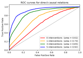
Figure 4: The ROC curves for identifying directed edges. See also figures 6 and 7 in the Supplementary Material.

5 CONCLUSION

We introduced $\sigma$-connection graphs ($\sigma$-CG) as a generalization of the d-connection graphs (d-CG) of [19] and extended the notion of $\sigma$-separation that was introduced in [12] to $\sigma$-CGs. We showed how $\sigma$-CGs behave under marginalisation and conditioning. This provides a graphical representation of how conditional independencies of modular structural causal models (mSCMs) behave under these operations. We provided a sufficient condition that allows constructing mSCMs and sampling from them. We extended the algorithm of [19] to deal with the more generally applicable notion of $\sigma$-separation instead of d-separation, thereby obtaining the first algorithm for causal discovery that can deal with cycles, non-linearities, latent confounders and a combination of data sets corresponding to observational and different interventional settings. We illustrated the effectiveness of the algorithm on simulated data. In this work, we restricted attention to (stochastic) perfect (“surgical”) interventions, but a straightforward extension to deal with other types of interventions and to generalize the idea of randomized controlled trials can be obtained by applying the JCI framework [23]. In future work we wish to improve our algorithm to also handle selection bias, become more scalable and apply it to real world data sets.

Acknowledgements

This work was supported by the European Research Council (ERC) under the European Union’s Horizon 2020 research and innovation programme (grant agreement 639466).

SUPPLEMENTARY MATERIAL

Appendix A $\Sigma$-CG UNDER MARGINALISATION AND CONDITIONING

 

Figure 5: A directed acyclic graph $G$ (top left) as the $\sigma$-connection graph ($\sigma$-CG) with the $\sigma$-equivalence classes $\{\{v_{1}\},\cdots,\{v_{6}\}\}$. We have the $\sigma$-separation: $\{v_{3}\}\operatorname*{{\,\perp\mkern-12.0mu\perp\,}}^{\sigma}_{G}\{v_{5}\}\operatorname*{|}\{v_{2},v_{4},v_{6}\}$. The combination of marginalizing out $v_{1}$ and conditioning on $v_{6}$ introduces cycles. Without keeping track of aboves $\sigma$-equivalence classes we would not get the corresponding $\sigma$-separation: $\{v_{3}\}\operatorname*{{\,\perp\mkern-12.0mu\perp\,}}^{\sigma}_{G^{\{v_{1}\}}_{\{v_{6}\}}}\{v_{5}\}\operatorname*{|}\{v_{2},v_{4}\}$ in the bottom right $\sigma$-CG.

Theorem A.1 ($\sigma$-Separation under Marginalisation).

Let $G$ be a $\sigma$-CG with set of nodes $V$ and $W,X,Y,Z\subseteq V$ subsets with $W=\{w\}$ and $w\notin X\cup Y\cup Z$. Then we have the equivalence:

$$X\operatorname*{{\,\perp\mkern-12.0mu\perp\,}}^{\sigma}_{G}Y\operatorname*{|}Z\;\iff\;X\operatorname*{{\,\perp\mkern-12.0mu\perp\,}}^{\sigma}_{G^{W}}Y\operatorname*{|}Z.$$

Proof.

If $\pi=x\cdots y$ is a $Z$-$\sigma$-open path in $G$ then every occurrence of $w$ in $\pi$ is as a non-collider. If we have $\cdots v\mathrel{\leavevmode\hbox to13.4pt{\vbox to0.4pt{\text{[drawing]}}}}w\mathrel{\leavevmode\hbox to14.4pt{\vbox to2.4pt{\text{[drawing]}}}}\cdots$ in $\pi$ and $v\notin Z$ then marginalising out $w$ keeps $\pi^{W}$ $Z$-$\sigma$-open in $G^{W}$. If $v\in Z$ then $v\in\sigma(w)$ by the $Z$-$\sigma$-openess. Since $\sigma(w)\in\mathcal{L}(G)$ is a loop we find elements $v_{i}\in\sigma(w)$, $r\geq 0$, $i=1,\dots r$, and a path

$$\cdots v\mathrel{\leavevmode\hbox to13.4pt{\vbox to0.4pt{\text{[drawing]}}}}v_{1}\mathrel{\leavevmode\hbox to13.4pt{\vbox to0.4pt{\text{[drawing]}}}}\cdots\mathrel{\leavevmode\hbox to13.4pt{\vbox to0.4pt{\text{[drawing]}}}}v_{r}\mathrel{\leavevmode\hbox to13.4pt{\vbox to0.4pt{\text{[drawing]}}}}w\mathrel{\leavevmode\hbox to14.4pt{\vbox to2.4pt{\text{[drawing]}}}}\cdots.$$

We do the same replacement on the right hand side of $w$ if necessary. Then marginalising this path w.r.t. $W$ gives a $Z$-$\sigma$-open path in $G^{W}$. This shows:

$$X\operatorname*{{\,\perp\mkern-12.0mu\perp\,}}^{\sigma}_{G^{W}}Y\operatorname*{|}Z\;\implies\;X\operatorname*{{\,\perp\mkern-12.0mu\perp\,}}^{\sigma}_{G}Y\operatorname*{|}Z.$$

Now let $x\cdots y$ be a $Z$-$\sigma$-open path in $G^{W}$. Then every edge lifts to a subpath in $G$ where $w$ only occurs as a non-collider. If a path $\cdots v\mathrel{\leavevmode\hbox to13.4pt{\vbox to0.4pt{\text{[drawing]}}}}z\cdots$ in $G^{W}$ with $z\in Z\cap\sigma(v)$ in $G$ comes from $\cdots v\mathrel{\leavevmode\hbox to13.4pt{\vbox to0.4pt{\text{[drawing]}}}}w\mathrel{\leavevmode\hbox to13.4pt{\vbox to0.4pt{\text{[drawing]}}}}z\cdots$ or $v\mathrel{\leavevmode\hbox to13.4pt{\vbox to0.4pt{\text{[drawing]}}}}w\mathrel{\leavevmode\hbox to13.4pt{\vbox to0.4pt{\text{[drawing]}}}}w\mathrel{\leavevmode\hbox to13.4pt{\vbox to0.4pt{\text{[drawing]}}}}z$ then we can, again since $\sigma(v)\in\mathcal{L}(G)$ is a loop, find nodes $v_{i}\in\sigma(v)$, $r\geq 0$, $i=1,\dots r$, and a path in $G$ of the form:

$$\cdots v\mathrel{\leavevmode\hbox to13.4pt{\vbox to0.4pt{\text{[drawing]}}}}v_{1}\mathrel{\leavevmode\hbox to13.4pt{\vbox to0.4pt{\text{[drawing]}}}}\cdots\mathrel{\leavevmode\hbox to13.4pt{\vbox to0.4pt{\text{[drawing]}}}}v_{r}\mathrel{\leavevmode\hbox to13.4pt{\vbox to0.4pt{\text{[drawing]}}}}z\cdots$$

which is in any case $Z$-$\sigma$-open in $G$ (whether $v$ or $z$ are colliders or not). So we can construct a $Z$-$\sigma$-open path in $G$ and we get:

$$X\operatorname*{{\,\perp\mkern-12.0mu\perp\,}}^{\sigma}_{G}Y\operatorname*{|}Z\;\implies\;X\operatorname*{{\,\perp\mkern-12.0mu\perp\,}}^{\sigma}_{G^{W}}Y\operatorname*{|}Z.$$

∎

Theorem A.2 ($\sigma$-Separation under Conditioning).

Let $G$ be a $\sigma$-CG with set of nodes $V$ and $C,X,Y,Z\subseteq V$ subsets with $C=\{c\}$ and $c\notin X\cup Y\cup Z$. Then we have the equivalence:

$$X\operatorname*{{\,\perp\mkern-12.0mu\perp\,}}^{\sigma}_{G}Y\operatorname*{|}Z\cup C\;\iff\;X\operatorname*{{\,\perp\mkern-12.0mu\perp\,}}^{\sigma}_{G_{C}}Y\operatorname*{|}Z.$$

Proof.

Let $C=\{c\}$. Let $\pi=x\cdots y$ be a $(Z\cup C)$-$\sigma$-open path in $G$ with a minimal number of arrowheads pointing to nodes in $C$. Then at $c$ (if $c$ occurs) there are no undirected edges. So we have the cases:

1. fork: $\cdots v_{1}\mathrel{\leavevmode\hbox to13.4pt{\vbox to0.4pt{\text{[drawing]}}}}c\mathrel{\leavevmode\hbox to13.4pt{\vbox to0.4pt{\text{[drawing]}}}}v_{2}\cdots$ in $G$ with $\sigma(v_{1})=\sigma(c)=\sigma(v_{2})$. Then $\cdots v_{1}\mathrel{\leavevmode\hbox to13.4pt{\vbox to0.4pt{\text{[drawing]}}}}v_{2}\cdots$ is in $G_{C}$ with $\sigma(v_{1})=\sigma(v_{2})=\sigma(c)$. So the triple situation for $v_{1}$, $v_{2}$ stays the same in $G_{C}$.

2. right chain: $\cdots v_{1}\begin{array}[]{c}\mathrel{\leavevmode\hbox to13.4pt{\vbox to0.4pt{\text{[drawing]}}}}\\[-10.0pt] \mathrel{\leavevmode\hbox to13.4pt{\vbox to0.4pt{\text{[drawing]}}}}\end{array}c\mathrel{\leavevmode\hbox to13.4pt{\vbox to0.4pt{\text{[drawing]}}}}v_{2}\cdots$ in $G$ with $\sigma(c)=\sigma(v_{2})$. Then $\cdots v_{1}\begin{array}[]{c}\mathrel{\leavevmode\hbox to13.4pt{\vbox to0.4pt{\text{[drawing]}}}}\\[-10.0pt] \mathrel{\leavevmode\hbox to13.4pt{\vbox to0.4pt{\text{[drawing]}}}}\end{array}v_{2}\dots$ is in $G_{C}$ with $\sigma(v_{2})=\sigma(c)$. So the triple situation for $v_{1}$, $v_{2}$ stays the same in $G_{C}$.

3. left chain: similar to right chain.

4. collider: $\cdots v_{1}\begin{array}[]{c}\mathrel{\leavevmode\hbox to13.4pt{\vbox to0.4pt{\text{[drawing]}}}}\end{array}c\begin{array}[]{c}\mathrel{\leavevmode\hbox to13.4pt{\vbox to0.4pt{\text{[drawing]}}}}\end{array}v_{2}\cdots$ in $G$. Then $\cdots v_{1}\mathrel{\leavevmode\hbox to13.4pt{\vbox to0.4pt{\text{[drawing]}}}}v_{2}\cdots$ is in $G_{C}$. So the triple situation for $v_{1}$, $v_{2}$ stays the same in $G_{C}$.

5. collider: $\cdots v_{1}\begin{array}[]{c}\mathrel{\leavevmode\hbox to13.4pt{\vbox to0.4pt{\text{[drawing]}}}}\end{array}c\begin{array}[]{c}\mathrel{\leavevmode\hbox to13.4pt{\vbox to0.4pt{\text{[drawing]}}}}\end{array}v_{2}\cdots$ in $G$ with $v_{1},v_{2}\notin Z$. Then $\cdots v_{1}\mathrel{\leavevmode\hbox to13.4pt{\vbox to0.4pt{\text{[drawing]}}}}v_{2}\cdots$ is in $G_{C}$ with $v_{1}$, $v_{2}$ non-collider. So it is $Z$-open at $v_{1}$, $v_{2}$.

6. collider: $\cdots\begin{array}[]{c}\mathrel{\leavevmode\hbox to13.4pt{\vbox to0.4pt{\text{[drawing]}}}}\\[-10.0pt] \mathrel{\leavevmode\hbox to13.4pt{\vbox to0.4pt{\text{[drawing]}}}}\\[-10.0pt] \mathrel{\leavevmode\hbox to13.4pt{\vbox to0.4pt{\text{[drawing]}}}}\end{array}v_{1}\begin{array}[]{c}\mathrel{\leavevmode\hbox to13.4pt{\vbox to0.4pt{\text{[drawing]}}}}\end{array}c\begin{array}[]{c}\mathrel{\leavevmode\hbox to13.4pt{\vbox to0.4pt{\text{[drawing]}}}}\\[-10.0pt] \mathrel{\leavevmode\hbox to13.4pt{\vbox to0.4pt{\text{[drawing]}}}}\end{array}v_{2}\cdots$ in $G$ with $v_{1}\in Z\cap\sigma(c)$. Since $\sigma(c)\in\mathcal{L}(G)$ is a loop there is a path in $G$ with $w_{i}\in\sigma(c)$, $r\geq 0$, $i=1,\dots,r$, of the form:

   $$\cdots\begin{array}[]{c}\mathrel{\leavevmode\hbox to13.4pt{\vbox to0.4pt{\text{[drawing]}}}}\\[-10.0pt] \mathrel{\leavevmode\hbox to13.4pt{\vbox to0.4pt{\text{[drawing]}}}}\\[-10.0pt] \mathrel{\leavevmode\hbox to13.4pt{\vbox to0.4pt{\text{[drawing]}}}}\end{array}v_{1}\mathrel{\leavevmode\hbox to13.4pt{\vbox to0.4pt{\text{[drawing]}}}}w_{1}\mathrel{\leavevmode\hbox to13.4pt{\vbox to0.4pt{\text{[drawing]}}}}w_{r}\mathrel{\leavevmode\hbox to13.4pt{\vbox to0.4pt{\text{[drawing]}}}}c\begin{array}[]{c}\mathrel{\leavevmode\hbox to13.4pt{\vbox to0.4pt{\text{[drawing]}}}}\\[-10.0pt] \mathrel{\leavevmode\hbox to13.4pt{\vbox to0.4pt{\text{[drawing]}}}}\end{array}v_{2}\cdots,$$

   which then is $(Z\cup C)$-$\sigma$-open. So the path

   $$\cdots\begin{array}[]{c}\mathrel{\leavevmode\hbox to13.4pt{\vbox to0.4pt{\text{[drawing]}}}}\\[-10.0pt] \mathrel{\leavevmode\hbox to13.4pt{\vbox to0.4pt{\text{[drawing]}}}}\\[-10.0pt] \mathrel{\leavevmode\hbox to13.4pt{\vbox to0.4pt{\text{[drawing]}}}}\end{array}v_{1}\mathrel{\leavevmode\hbox to13.4pt{\vbox to0.4pt{\text{[drawing]}}}}w_{1}\mathrel{\leavevmode\hbox to13.4pt{\vbox to0.4pt{\text{[drawing]}}}}\cdots w_{r}\begin{array}[]{c}\mathrel{\leavevmode\hbox to13.4pt{\vbox to0.4pt{\text{[drawing]}}}}\\[-10.0pt] \mathrel{\leavevmode\hbox to13.4pt{\vbox to0.4pt{\text{[drawing]}}}}\end{array}v_{2}\cdots$$

   is then $Z$-$\sigma$-open in $G_{C}$.

7. collider: $\cdots v_{1}\begin{array}[]{c}\mathrel{\leavevmode\hbox to13.4pt{\vbox to0.4pt{\text{[drawing]}}}}\end{array}c\begin{array}[]{c}\mathrel{\leavevmode\hbox to13.4pt{\vbox to0.4pt{\text{[drawing]}}}}\end{array}v_{2}\cdots$ in $G$ with $v_{1}\notin Z$. Then $\cdots v_{1}\mathrel{\leavevmode\hbox to13.4pt{\vbox to0.4pt{\text{[drawing]}}}}v_{2}\cdots$ is in $G_{C}$ and $Z$-open.

8. collider: as before with $v_{1}$ and $v_{2}$ swapped. Same arguments.

These cover all cases and we have shown:

$$X\operatorname*{{\,\perp\mkern-12.0mu\perp\,}}_{G_{C}}^{\sigma}Y\operatorname*{|}Z\;\implies\;X\operatorname*{{\,\perp\mkern-12.0mu\perp\,}}_{G}^{\sigma}Y\operatorname*{|}Z\cup C.$$

Now let $x\cdots y$ be a $Z$-open path in $G_{C}$. Then the rules for conditioning lift every edge in $G_{C}$ to an edge or triple in $G$, where the triple situation for $c$ is $C$-$\sigma$-open and where the triple situation for the endnodes stays the same. So it is clearly $(Z\cup C)$-open in $G$. This shows:

$$X\operatorname*{{\,\perp\mkern-12.0mu\perp\,}}_{G}^{\sigma}Y\operatorname*{|}Z\cup C\;\implies\;X\operatorname*{{\,\perp\mkern-12.0mu\perp\,}}_{G_{C}}^{\sigma}Y\operatorname*{|}Z.$$

∎

Appendix B THE $\Sigma$-SEPARATION CRITERION FOR MSCMS

The trick to prove the $\sigma$-separation criterion is to transform the $\sigma$-connection graph $G$ of an mSCM, which has no undirected edges and can be seen as a directed mixed graph (DMG), into an acyclic directed mixed graph (ADMG) that encodes the same conditional independencies in terms of the well known d-separation. This also shows that every $\sigma$-separation-equivalence-class contains an acyclic graph (if one only looks at the observational distributions). Caution: the constructed ADMG is not well-behaved under marginalisation or interventions. We will refer to the d-separation criterion as the directed global Markov property (dGMP) and to the $\sigma$-separation criterion as the generalized directed global Markov property (gdGMP) in the following.

Lemma B.1.

Let $G=(V,E,H)$ be an acyclic directed mixed graph (ADMG) and $(X_{v})_{v\in V}$ be random variables that satisfy the dGMP w.r.t. $G$. Let $E_{w}$ be a random variable independent of $(X_{v})_{v\in V}$ and $X_{w}$ be another random variable, $w\notin V$, given by a functional relation:

$$X_{w}=f\big{(}(X_{v})_{v\in P},E_{w}\big{)},$$

where $P\subseteq V$ is a subset of nodes. Let $G^{\prime}=(V^{\prime},E^{\prime},H^{\prime})$ be the ADMG with set of nodes $V^{\prime}:=V\cup\{w\}$, set of edges $E^{\prime}:=E\cup\{v\mathrel{\leavevmode\hbox to13.4pt{\vbox to0.4pt{\text{[drawing]}}}}w|v\in P\}$ and set of bidirected edges $H^{\prime}:=H$. Then $G\subseteq G^{\prime}$ is an ancestral sub-ADMG and $(X_{v})_{v\in V^{\prime}}$ satisfies the dGMP w.r.t. $G^{\prime}$.

Proof.

Since $w$ is a childless node in $G^{\prime}$ clearly $G^{\prime}$ is acyclic, $\mathrm{Pa}^{G^{\prime}}(w)=P$ and $G\subseteq G^{\prime}$ is an ancestral sub-ADMG. So there exists a topological order $<$ for $G^{\prime}$ such that $w$ is the last element. Since for an ADMG the directed global Markov property (dGMP) is equivalent to the ordered local Markov property (oLMP) w.r.t. any topological order (see [12, 28]) we only need to check the local independence:

$$\{w\}\operatorname*{{\,\perp\mkern-12.0mu\perp\,}}_{\mathbb{P}}A\setminus\{w\}\operatorname*{|}\partial_{A^{\mathrm{mor}}}(w)$$

for every ancestral $A\subseteq G^{\prime}$ with $w\in A$. Since $\partial_{A^{\mathrm{mor}}}(w)=\mathrm{Pa}^{G^{\prime}}(w)=P$ and $A\setminus\{w\}\subseteq V$ the statement follows directly from the implication:

$$\begin{split}&E_{w}\operatorname*{{\,\perp\mkern-12.0mu\perp\,}}_{\mathbb{P}}(X_{v})_{v\in V}\;\implies\\ &f\big{(}(X_{v})_{v\in P},E_{w}\big{)}\operatorname*{{\,\perp\mkern-12.0mu\perp\,}}_{\mathbb{P}}(X_{v})_{v\in A\setminus\{w\}}\operatorname*{|}(X_{v})_{v\in P}.\end{split}$$

∎

Theorem B.2.

Let $G=(V,E,H)$ be a directed mixed graph (DMG) and $\mathcal{S}(G)$ the set of its strongly connected components. Assume that we have:

1. random variables $(X_{v})_{v\in V}$,

2. random variables $(E_{v})_{v\in V}$ that jointly satisfy the dGMP w.r.t. the bidirected graph $(V,\emptyset,H)$, i.e. for every $W,Y\subseteq V$ we have the implication:

   $$W\operatorname*{{\,\perp\mkern-12.0mu\perp\,}}^{d}_{(V,\emptyset,H)}Y\;\implies\;(E_{v})_{v\in W}\operatorname*{{\,\perp\mkern-12.0mu\perp\,}}_{\mathbb{P}}(E_{v})_{v\in Y},$$

3. a tuple of functions $(g_{S})_{S\in\mathcal{S}(G)}$ indexed by the strongly connected components $S$ of $G$,

such that we have the following equations for $S\in\mathcal{S}(G)$:

$$(X_{v})_{v\in S}=g_{S}\big{(}(X_{w})_{w\in\mathrm{Pa}^{G}(S)\setminus S},(E_{w})_{w\in S}\big{)}.$$

Then $(X_{v})_{v\in V}$ satisfy the general directed global Markov property (gdGMP) w.r.t. the DMG $G$, i.e. for every three subsets $W,Y,Z\subseteq V$ we have the implication:

$$W\operatorname*{{\,\perp\mkern-12.0mu\perp\,}}^{\sigma}_{G}Y\operatorname*{|}Z\;\implies\;(X_{v})_{v\in W}\operatorname*{{\,\perp\mkern-12.0mu\perp\,}}_{\mathbb{P}}(X_{v})_{v\in Y}\operatorname*{|}(X_{v})_{v\in Z}.$$

Proof.

By assumption we have that $(E_{v})_{v\in V}$ satisfies the dGMP w.r.t. the ADMG $(V,\emptyset,H)$. By lemma B.1 we can inductively add:

$$X_{v}=g_{S,v}\big{(}(X_{w})_{\mathrm{Pa}^{G}(S)\setminus S},(E_{w})_{w\in S}\big{)}$$

for $v\in V$ where $S=\mathrm{Sc}^{G}(v)$. We then finally get an ADMG $G^{\prime}$ with nodes $(E_{v})_{v\in V}$ and $(X_{v})_{v\in V}$ that satisfy the dGMP w.r.t. this $G^{\prime}$. This implies that for $W,Y,Z\subseteq V$ we have:

$$W\operatorname*{{\,\perp\mkern-12.0mu\perp\,}}^{d}_{G^{\prime}}Y\operatorname*{|}Z\;\stackrel{{\scriptstyle}}{{\implies}}\;(X_{v})_{v\in W}\operatorname*{{\,\perp\mkern-12.0mu\perp\,}}_{\mathbb{P}}(X_{v})_{v\in Y}\operatorname*{|}(X_{v})_{v\in Z}.$$

It is thus left to show that we also have the implication:

$$W\operatorname*{{\,\perp\mkern-12.0mu\perp\,}}^{\sigma}_{G}Y\operatorname*{|}Z\;\stackrel{{\scriptstyle}}{{\implies}}\;W\operatorname*{{\,\perp\mkern-12.0mu\perp\,}}^{d}_{G^{\prime}}Y\operatorname*{|}Z.$$

For this it is enough to show that every $Z$-d-open path $\pi^{\prime}$ from $W$ to $Y$ in $G^{\prime}$ lifts to a $Z$-$\sigma$-open path $\pi$ from $W$ to $Y$ in $G$. The construction is straightforward. For details see [12]. ∎

Corollary B.3.

The observed variables $(X_{v})_{v\in V}$ of any mSCM $M=(G^{+},\mathcal{X},\mathbb{P},g)$, $G^{+}=(U\dot{\cup}V,E^{+})$, satisfy the $\sigma$-separation criterion w.r.t. the induced $\sigma$-connection graph ($\sigma$-CG) $G$.

Proof.

For $v\in V$ we put $E_{v}:=(E_{u})_{\begin{subarray}{c}u\in U\\ v\in\mathrm{Ch}^{G^{+}}(u)\end{subarray}}$. The $(E_{v})_{v\in V}$ then entail the conditional independence relations implied by d-separation of the bidirected graph $(V,\emptyset,H)$. Furthermore, for $S\in\mathcal{S}(G)$ we have equations:

$$X_{S}=g_{S}(X_{\mathrm{Pa}^{G}(S)\setminus S},E_{S}).$$

The claim then directly follows from B.2. ∎

As a motivation for future work on selection bias we state the following direct corollary.

Corollary B.4 (mSCM with context).

Let $M=(G^{+},\mathcal{X},\mathbb{P},g)$ be a mSCM with $G^{+}=(U\dot{\cup}V,E^{+})$ and $C\subseteq V$ a subset. Let $G_{C}=(G^{+})^{U}_{C}$ be the induced $\sigma$-CG of $M$ conditioned on $C$. Then the observed variables $(X_{v})_{v\in V\setminus C}$ satisfy the $\sigma$-separation criterion w.r.t. $G_{C}$ and w.r.t. the regular conditional probability distribution $\mathbb{P}^{|X_{C}=x_{C}}$ given $X_{C}=x_{C}$ (for $\mathbb{P}^{X_{C}}$-almost-all values $x_{C}\in\mathcal{X}_{C}$): For all subsets $W,Y,Z\subseteq V\setminus C$ we have the implication:

$$W\operatorname*{{\,\perp\mkern-12.0mu\perp\,}}^{\sigma}_{G_{C}}Y\operatorname*{|}Z\;\implies\;X_{W}\operatorname*{{\,\perp\mkern-12.0mu\perp\,}}_{\mathbb{P}^{|X_{C}=x_{C}}}X_{Y}\operatorname*{|}X_{Z}.$$

Proof.

The lhs is equivalent to $W\operatorname*{{\,\perp\mkern-12.0mu\perp\,}}^{\sigma}_{G}Y\operatorname*{|}Z\cup C$ (see Theorem 2.20, Theorem A.2, resp.) and this implies $X_{W}\operatorname*{{\,\perp\mkern-12.0mu\perp\,}}_{\mathbb{P}}X_{Y}\operatorname*{|}X_{Z},X_{C}$ (see Theorem 2.14, Corollary B.3, resp.), which implies the claim on the rhs (for $\mathbb{P}^{X_{C}}$-almost-all values $x_{C}\in\mathcal{X}_{C}$). ∎

The last corollary can be used as a starting point for conditional independence constraint-based causal discovery in the presence of (unknown) selection bias given by the unknown context $C$ and $x_{C}\in\mathcal{X}_{C}$ (in addition to non-linear functional relations, cycles and latent confounders etc.).

Appendix C NEURAL NETWORKS AS MSCMS

For constructing causal mechanisms we could use any parametric or non-parametric family of functions. Since we want to stay as general as possible and also make use of the practical advantages of parametric models we represent/approximate the structural functions $g_{\{v\}}$, $v\in V$ by universal approximators. A well known class of universal approximators are neural networks (see e.g. [16]). A neural network is a function that is constructed from several compositions of linear maps and a fixed one-dimensional activation function $h$. A sufficient condition to have the universal approximation property is if one assumes $h$ be continuous, non-polynomial and piecewise differentiable. A further advantage of neural networks is that the hidden units (given by composition of functions $z\mapsto h(w^{T}z+b)$) can be interpreted as intermediate variables of an extended structural causal model. This means that by modelling the hidden units of every $g_{\{v\}}$ explicitely as a node in an extended graph we can restrict—for the analysis purposes here—to this extended setting, where now the functions $g_{\{v\}}$ (the index $\{v\}$ refers to the trivial loop) are of the form:

$$\begin{array}[]{rcl}&&g_{\{v\}}(x_{\mathrm{Pa}^{G^{+}}(v)\setminus\{v\}})\\ &=&h\left(\sum_{k\in\mathrm{Pa}^{G^{+}}(v)\setminus\{v\}}A_{v,k}\cdot x_{k}+b_{v}\right),\end{array}$$

with weights $A_{v,k}$ and biases $b_{v}$.

Further note that introducing or marginalizing intermediate variables will not change the outcome of the $\sigma$-separation criterion defined in Definition 2.10, Theorem 2.14, and Theorem 2.20 (also see [12]). So also this part is compatible with our theory.

Theorem C.1.

The conditions for the contractiveness of the iterations scheme from subsection 4.1 are satisfied if the following three points hold:

1. $\sup_{z}|h^{\prime}(z)|\leq C$ with $0<C<\infty$, and

2. $A_{v,k}:=0$ for $k\notin\mathrm{Pa}^{G^{+}}(v)\setminus\{v\}$, and

3. $||(A_{v,k})_{v,k\in S}||<\frac{1}{C}$ for every non-trivial loop $S\subseteq G$, where $||\cdot||$ can be one of the matrix norms: $||\cdot||_{p}$, $p\geq 1$, or $||\cdot||_{\infty}$.

In this case the functions $(g_{\{v\}})_{v\in V}$ will constitute a well-defined mSCM.

Note that we can put $C=1$ for popular activation functions $h(z)$ like $\tanh(z)$, $\mathrm{ReLU}(z)=\max(0,z)$, $\sigma(z)=\frac{1}{1+\exp(-z)}$, LeakyRelu, SoftPlus$(z)=\ln(1+e^{z})$, etc..
Further note that by using one of these activation functions $h(z)$ and $||\cdot||=||\cdot||_{\infty}$ all the conditions are satisfied if we choose the $A_{v,k}$ such that for all $v\in V$:

$$\begin{array}[]{rcl}&&\sum_{k\in\mathrm{Pa}^{G^{+}}(v)\setminus\{v\}}|A_{v,k}|<1\\ &\text{ and }&A_{v,k}:=0\quad\text{ for }\quad k\notin\mathrm{Pa}^{G^{+}}(v)\setminus\{v\}.\end{array}$$

Furthermore, we can then iterate the whole system for given error value $x_{U}$ and initialization $x_{V}^{(0)}$:

$$\begin{array}[]{rcl}x_{V}^{(t+1)}&:=&(g_{\{v\}})_{v\in V}(x_{V}^{(t)},x_{U})\\ &=&h\left(A_{V^{+}}\cdot({x_{V}^{(t)}\atop x_{U}})+b_{V}\right)\end{array}$$

and reach a unique fixed point $x_{V}$. This analyis also holds if we have the error variables outside of the activation function as additive noise.

Proof.

For a non-trivial loop $S\subseteq G$ we want to show that for every value $x_{\mathrm{Pa}^{G^{+}}(S)\setminus S}$ and initialization $x_{S}^{(0)}$ the iteration (using vector and matrix notations):

$$\begin{array}[]{rcl}&&x_{S}^{(t+1)}:=\\ &&h\left(A_{\mathrm{Pa}^{G^{+}}(S)\cup S}\cdot(x_{S}^{(t)},x_{\mathrm{Pa}^{G^{+}}(S)\setminus S})^{T}+b_{S}\right)\end{array}$$

converges to a unique point $x_{S}$ (for $t\to\infty$) under the three stated assumptions in the text.
For applying Banach’s fixed point theorem we need to show that for every value $x_{\mathrm{Pa}^{G^{+}}(S)\setminus S}$ we have a bounded partial Jacobian ($S$ a non-trivial loop):

$$\sup_{x_{S}}||J_{S}(x_{\mathrm{Pa}^{G^{+}}(S)\cup S})||\leq L(x_{\mathrm{Pa}^{G^{+}}(S)\setminus S})<1$$

where $L(x_{\mathrm{Pa}^{G^{+}}(S)\setminus S})$ is a constant smaller than $1$ and $||\cdot||$ is a suitable matrix norm. In our case we have:

$$\begin{array}[]{rcl}&&J_{S}(x_{\mathrm{Pa}^{G^{+}}(S)\cup S})\\ &:=&\left(\frac{\partial g_{\{v\}}}{\partial x_{k}}\right)_{v,k\in S}(x_{\mathrm{Pa}^{G^{+}}(S)\cup S})\\ &=&\nabla_{x_{S}}h\left(A_{\mathrm{Pa}^{G^{+}}(S)\cup S}\cdot\left({x_{S}\atop x_{\mathrm{Pa}^{G^{+}}(S)\setminus S}}\right)+b_{S}\right)\\ &=&\left(h^{\prime}\left(\sum_{j\in\mathrm{Pa}^{G^{+}}(v)\setminus\{v\}}A_{v,j}\cdot x_{j}+b_{v}\right)\right.\\ &&\left.\quad\cdot A_{v,k}\cdot\mathds{1}_{k\in\mathrm{Pa}^{G^{+}}(v)\setminus\{v\}}\right)_{v,k\in S}\\ &=&\operatorname*{\mathrm{diag}}(h^{\prime})\cdot\left(A_{S}\odot\mathds{1}_{S}\right).\end{array}$$

Here $\operatorname*{\mathrm{diag}}(h^{\prime})$ refers to the diagonal matrix with the corresponding values of $h^{\prime}$ and $\mathds{1}_{S}$ is the adjacency matrix as indicated on the line above.
If $|h^{\prime}(z)|\leq C<\infty$ and $||\cdot||$ is either $||\cdot||_{p}$, $p\geq 1$, or $||\cdot||_{\infty}$ then $||\operatorname*{\mathrm{diag}}(h^{\prime})||\leq C$. If, furthermore, $||A_{S}\odot\mathds{1}_{S}||<\frac{1}{C}$ then we get:

$$\begin{array}[]{rcl}||J_{S}||&\leq&||\operatorname*{\mathrm{diag}}(h^{\prime})||\cdot||A_{S}\odot\mathds{1}_{S}||\\ &\leq&C\cdot||A_{S}\odot\mathds{1}_{S}||=:L\\ &<&C\cdot\frac{1}{C}\\ &=&1.\end{array}$$

Note that we can represent $A\odot\mathds{1}$ in a single matrix $A$ if we put $A_{v,k}:=0$ whenever $k\notin\mathrm{Pa}^{G^{+}}(v)\setminus\{v\}$. From the above then follows that the map of the iteration scheme becomes contractive and the series thus converges to a unique fixed point $x_{S}$. $g_{S}$ can then be defined via:

$$g_{S}(x_{\mathrm{Pa}^{G^{+}}(S)\setminus S}):=x_{S}.$$

The system $(g_{S})_{S\in\mathcal{L}(G)}$ is also compatible. Indeed, the convergence shows that the above element $(x_{\mathrm{Pa}^{G^{+}}(S)\setminus S},x_{S})$ simultaneously solves the system $x_{v}=g_{\{v\}}(x_{\mathrm{Pa}^{G^{+}}(v)\setminus\{v\}})$, $v\in S$. So for a loop $S^{\prime}\subseteq S$ the corresponding components $(x_{\mathrm{Pa}^{G^{+}}(S^{\prime})\setminus S^{\prime}},x_{S^{\prime}})$ simultaneously solves the system $x_{v}=g_{\{v\}}(x_{\mathrm{Pa}^{G^{+}}(v)\setminus\{v\}})$, $v\in S^{\prime}$. Since also the solution for the loop $S^{\prime}$ is unique we get:

$$g_{S^{\prime}}(x_{\mathrm{Pa}^{G^{+}}(S^{\prime})\setminus S^{\prime}})=x_{S^{\prime}},$$

which shows the compatibility. The measurability of this map follows from a measurable choice theorem (see [2]) as explained in [3]. ∎

If we want to uniformly sample weights for the parent nodes one can use the following:

Remark C.2 (See [1]).

To uniformly sample from the $d$-dimensional $L_{p}$-ball $B^{d}_{p}:=\{x\in\mathbb{R}^{d}:||x||_{p}\leq 1\}$ we can sample i.i.d. $y_{1},\dots,y_{d}\sim p(t)=\frac{1}{2\Gamma(1+\frac{1}{p})}e^{-|t|^{p}}$, $t\in\mathbb{R}$ and $z\sim p(s)=e^{-s}$, $s\geq 0$. Then $x=\frac{(y_{1},\dots,y_{d})^{T}}{\left(\sum_{j=1}^{d}|y_{j}|^{p}+z\right)^{1/p}}$ is uniformly sampled from $B^{d}_{p}$.

Appendix D MORE DETAILS ON THE ALGORITHM

D.1 SCORING FEATURES

In order to score features, which can be defined as Boolean functions of the causal graph $G$, we define a modified loss function

$$\begin{split}&\mathcal{L}(G,S,f):=\\ &\sum_{(w_{j},y_{j},Z_{j},I_{j},\lambda_{j})\in S}\lambda_{j}(\mathds{1}_{\lambda_{j}>0}-\mathds{1}_{w_{j}\operatorname*{{\,\perp\mkern-12.0mu\perp\,}}^{\sigma}_{G_{\mathrm{do}(I_{j})}}y_{j}\operatorname*{|}Z_{j}}\mathds{1}_{f(G)})\end{split}$$ (4)

[21] proposed to score the confidence of a feature with

$$\begin{split}C(S,f):=&\min_{G\in\mathbb{G}(V)}\mathcal{L}(G,S,\lnot f)\\ &-\min_{G\in\mathbb{G}(V)}\mathcal{L}(G,S,f).\end{split}$$ (5)

They showed that this scoring method is sound for oracle inputs.

Theorem D.1.

For any feature $f$, the confidence score $C(S,f)$ of (5) is sound for oracle inputs with infinite weights. In other words, $C(S,f)=\infty$ if $f$ is identifiable from the inputs, $C(S,f)=-\infty$ if $\lnot f$ is identifiable from the inputs, and $C(S,f)=0$ if $f$ is unidentifiable from the inputs.

Furthermore, they showed that the scoring method is asymptotically consistent under a consistency condition on the statistical independence test.

Theorem D.2.

Assume that the weights are asymptotically consistent, meaning that

$$\log p_{N}-\log\alpha_{N}\stackrel{{\scriptstyle P}}{{\to}}\begin{cases}-\infty&H_{1}\\ +\infty&H_{0},\end{cases}$$ (6)

as the number of samples $N\to\infty$, where the null hypothesis $H_{0}$ is independence and the alternative hypothesis $H_{1}$ is dependence. Then for any feature $f$, the confidence score $C(S,f)$ of (5) is asymptotically consistent, i.e., $C(S,f)\to\infty$ in probability if $f$ is identifiably true, $C(S,f)\to-\infty$ in probability if $f$ is identifiably false, and $C(S,f)\to 0$ in probability otherwise.

By using the scoring method of [21] as explained above, our algorithm inherits these desirable properties.

D.2 ENCODING IN ANSWER SET PROGRAMMING

In order to test whether a causal graph $G$ entails a certain independence, we create a computation graph of $\sigma$-connection graphs. A computation graph of $\sigma$-connection graphs is a DAG with $\sigma$-connection graphs as nodes, and directed edges that correspond with the operations of conditioning and marginalisation. The “source node” of an encoding DAG is an (intervened) causal graph. The “sink” nodes are $\sigma$-connection graphs that consist of only two variables (because all other variables have been conditioned or marginalised out) that can be reached from the source node by applying a sequence of conditioning and marginalisation operations. Testing a $\sigma$-separation statement in the intervened causal graph reduces to testing for adjacency in the corresponding sink node.

Since interventions and conditioning do not commute, one has to take care to employ these operations in the right ordering. We define the computation graph in such a way that intervention operations are performed first, followed by marginalisations, and finally conditioning operations. At each stage, we always remove the node with the highest possible label first, which means that our computation graph is actually a computation tree.

Below we provide the source code of the essential part of the algorithm, using the ASP syntax for clingo 4. It is based upon the source code provided by [19]. The differences to [19], i.e. of $\sigma$-separation vs. d-separation, are indicated with “(sigma)” in the comments, i.e. at lines 100, 128, 138. Note that the main difference between the encoding of d-separation and $\sigma$-separation is that in the non-collider case (see definition 2.9) we need to check in which strongly connected component $\sigma(v)$ the non-collider node lies in comparison to its adjacent nodes. This boils down to checking ancestral relations. Since the $\sigma$-structure is inherited in a trivial fashion during the marginalisation and conditioning operations, it only needs to be found once (namely in the original $\sigma$-CG induced by the mSCM).

We used the state-of-the-art ASP solver clingo 4 [13] in our experiments to run the ASP program.

⬇

1%%%%%%%%%% COMPUTATION GRAPH %%%%%%%%%%%%%%%%%%%%%%%%%%%%%%%

2

3% preliminaries

4node(0..nrnodes-1).

5set(0..2**nrnodes-1).

6ismember(M,Z) :- set(M), node(Z), M & (2**Z) != 0.

7

8% first intervene, then marginalize, then condition;

9% always remove the node with the highest possible label first

10intervene(0,Jsub,Z,J,0) :- node(Z), set(J), set(Jsub),

11 ismember(J,Z), not ismember(Jsub,Z),

12 (Jsub + 2**Z) == J, 2**Z > Jsub.

13marginalize(0,J,Msub,Z,M) :- node(Z), set(M), set(J), set(Msub),

14 ismember(M,Z), not ismember(Msub,Z),

15 (Msub + 2**Z) == M, 2**Z > Msub.

16condition(Csub,Z,C,J,M) :- node(Z), set(M), set(C), set(J), set(Csub),

17 (C & M) == 0, ismember(C,Z), not ismember(Csub,Z),

18 (Csub + 2**Z) == C, 2**Z > Csub.

19

20% guess (generate all possible directed mixed graphs)

21{ edge(X,Y) } :- node(X), node(Y), X != Y.

22{ conf(X,Y) } :- node(X), node(Y), X < Y.

23

24% source node in computation graph

25th(X,Y,0,0,0) :- edge(X,Y).

26hh(X,Y,0,0,0) :- conf(X,Y).

27

28% ancestral relations after perfect (surgical) intervention on J

29ancestor(X,Y,J) :- th(X,Y,0,J,0), X!=Y, node(X), node(Y), set(J).

30ancestor(X,Y,J) :- ancestor(X,Z,J), ancestor(Z,Y,J),

31 X!=Y, X!=Z, Y!=Z,

32 node(X), node(Y), node(Z), set(J).

33

34

35%%%%%%%%%% INTERVENTION %%%%%%%%%%%%%%%%%%%%%%%%%%%%%%%%%%%%

36

37tt(X,Y,C,J,M) :- tt(X,Y,C,Jsub,M),

38 X <= Y,

39 not ismember(C,X), not ismember(C,Y),

40 not ismember(M,X), not ismember(M,Y),

41 node(X),node(Y),

42 intervene(C,Jsub,Z,J,M).

43

44th(X,Y,C,J,M) :- th(X,Y,C,Jsub,M),

45 X != Y,

46 not ismember(J,Y),

47 not ismember(C,X), not ismember(C,Y),

48 not ismember(M,X), not ismember(M,Y),

49 node(X),node(Y),

50 intervene(C,Jsub,Z,J,M).

51

52hh(X,Y,C,J,M) :- hh(X,Y,C,Jsub,M),

53 X < Y,

54 not ismember(J,Y), not ismember(J,X),

55 not ismember(C,X), not ismember(C,Y),

56 not ismember(M,X), not ismember(M,Y),

57 node(X),node(Y),

58 intervene(C,Jsub,Z,J,M).

59

60%%%%%%%%%%%%%%%%%%%%%%%%%%%%%%%%%%%%%%%%%%%%%%%%%%%%%%%%%%

61

62

63%%%%%%%%%% CONDITIONING %%%%%%%%%%%%%%%%%%%%%%%%%%%%%%%%%%

64

65%% X---Y => X---Y

66tt(X,Y,C,J,M) :- tt(X,Y,Csub,J,M),

67 X <= Y,

68 not ismember(C,X), not ismember(C,Y),

69 not ismember(M,X), not ismember(M,Y),

70 node(X),node(Y),

71 condition(Csub,Z,C,J,M).

72

73%% X-->Z<--Y => X---Y

74tt(X,Y,C,J,M) :- th(X,Z,Csub,J,M),th(Y,Z,Csub,J,M),

75 X <= Y,

76 not ismember(C,X), not ismember(C,Y),

77 not ismember(M,X), not ismember(M,Y),

78 node(X),node(Y),

79 condition(Csub,Z,C,J,M).

80

81%%%%%%%%%%%%%%%%%%%%%%%%%%%%%%%%%%%%%%%%%%%%%%%%%%%%%%%%%%%%

82

83%% X-->Y => X-->Y

84th(X,Y,C,J,M) :- th(X,Y,Csub,J,M),

85 X != Y,

86 not ismember(C,X), not ismember(C,Y),

87 not ismember(M,X), not ismember(M,Y),

88 node(X),node(Y),

89 condition(Csub,Z,C,J,M).

90

91%% X-->Z<->Y => X-->Y

92th(X,Y,C,J,M) :- th(X,Z,Csub,J,M),

93 { hh(Z,Y,Csub,J,M); hh(Y,Z,Csub,J,M) } >= 1,

94 X != Y,

95 not ismember(C,X), not ismember(C,Y),

96 not ismember(M,X), not ismember(M,Y),

97 node(X),node(Y),

98 condition(Csub,Z,C,J,M).

99

100%% X-->Z-->Y (anc of Z) => X-->Y (sigma)

101th(X,Y,C,J,M):- th(X,Z,Csub,J,M), th(Z,Y,Csub,J,M),

102 ancestor(Y,Z,J),

103 X != Y,

104 not ismember(C,X), not ismember(C,Y),

105 not ismember(M,X), not ismember(M,Y),

106 node(X),node(Y),node(Z),

107 condition(Csub,Z,C,J,M).

108

109%%%%%%%%%%%%%%%%%%%%%%%%%%%%%%%%%%%%%%%%%%%%%%%%%%%%%%%%%%%%

110

111%% X<->Y => X<->Y

112hh(X,Y,C,J,M) :- hh(X,Y,Csub,J,M),

113 X < Y,

114 not ismember(C,X), not ismember(C,Y),

115 not ismember(M,X), not ismember(M,Y),

116 node(X),node(Y),

117 condition(Csub,Z,C,J,M).

118

119%% X<->Z<->Y => X<->Y

120hh(X,Y,C,J,M) :- { hh(Z,X,Csub,J,M); hh(X,Z,Csub,J,M) } >= 1,

121 { hh(Z,Y,Csub,J,M); hh(Y,Z,Csub,J,M) } >= 1,

122 X < Y,

123 not ismember(C,X), not ismember(C,Y),

124 not ismember(M,X), not ismember(M,Y),

125 node(X),node(Y),

126 condition(Csub,Z,C,J,M).

127

128%% X<->Z-->Y (anc of Z) => X<->Y (sigma)

129hh(X,Y,C,J,M) :- { hh(Z,X,Csub,J,M); hh(X,Z,Csub,J,M) } >= 1,

130 th(Z,Y,Csub,J,M),

131 ancestor(Y,Z,J),

132 X < Y,

133 not ismember(C,X), not ismember(C,Y),

134 not ismember(M,X), not ismember(M,Y),

135 node(X),node(Y),node(Z),

136 condition(Csub,Z,C,J,M).

137

138%% (anc of Z) X<--Z-->Y (anc of Z) => X<->Y (sigma)

139hh(X,Y,C,J,M) :- th(Z,X,Csub,J,M), th(Z,Y,Csub,J,M),

140 ancestor(X,Z,J),

141 ancestor(Y,Z,J),

142 X < Y,

143 not ismember(C,X), not ismember(C,Y),

144 not ismember(M,X), not ismember(M,Y),

145 node(X),node(Y),node(Z),

146 condition(Csub,Z,C,J,M).

147

148%%%%%%%%%%%%%%%%%%%%%%%%%%%%%%%%%%%%%%%%%%%%%%%%%%%%%%%%%%%%

149

150

151%%%%%%%%%% MARGINALIZATION %%%%%%%%%%%%%%%%%%%%%%%%%%%%%%%%%

152

153%% X---Y => X---Y

154tt(X,Y,C,J,M) :- tt(X,Y,C,J,Msub),

155 X <= Y,

156 not ismember(C,X), not ismember(C,Y),

157 not ismember(M,X), not ismember(M,Y),

158 node(X),node(Y),

159 marginalize(C,J,Msub,Z,M).

160

161%% X-->Z---Y => X---Y

162tt(X,Y,C,J,M) :- th(X,Z,C,J,Msub),

163 { tt(Z,Y,C,J,Msub); tt(Y,Z,C,J,Msub) } >= 1,

164 X <= Y,

165 not ismember(C,X), not ismember(C,Y),

166 not ismember(M,X), not ismember(M,Y),

167 node(X),node(Y),

168 marginalize(C,J,Msub,Z,M).

169

170%% X---Z<--Y => X---Y

171tt(X,Y,C,J,M) :- { tt(X,Z,C,J,Msub); tt(Z,X,C,J,Msub) } >= 1,

172 th(Y,Z,C,J,Msub),

173 X <= Y,

174 not ismember(C,X), not ismember(C,Y),

175 not ismember(M,X), not ismember(M,Y),

176 node(X),node(Y),

177 marginalize(C,J,Msub,Z,M).

178

179%% X---Z---Y => X---Y

180tt(X,Y,C,J,M) :- { tt(X,Z,C,J,Msub); tt(Z,X,C,J,Msub) } >= 1,

181 { tt(Z,Y,C,J,Msub); tt(Y,Z,C,J,Msub) } >= 1,

182 X <= Y,

183 not ismember(C,X), not ismember(C,Y),

184 not ismember(M,X), not ismember(M,Y),

185 node(X),node(Y),

186 marginalize(C,J,Msub,Z,M).

187

188%% X-->Z---Z<--Y => X---Y

189tt(X,Y,C,J,M) :- th(X,Z,C,J,Msub),th(Y,Z,C,J,Msub),tt(Z,Z,C,J,Msub),

190 X <= Y,

191 not ismember(C,X), not ismember(C,Y),

192 not ismember(M,X), not ismember(M,Y),

193 node(X),node(Y),

194 marginalize(C,J,Msub,Z,M).

195

196%%%%%%%%%%%%%%%%%%%%%%%%%%%%%%%%%%%%%%%%%%%%%%%%%%%%%%%%%%%%

197

198%% X-->Y => X-->Y

199th(X,Y,C,J,M) :- th(X,Y,C,J,Msub),

200 X != Y,

201 not ismember(C,X), not ismember(C,Y),

202 not ismember(M,X), not ismember(M,Y),

203 node(X),node(Y),

204 marginalize(C,J,Msub,Z,M).

205

206%% X-->Z-->Y => X-->Y

207th(X,Y,C,J,M) :- th(X,Z,C,J,Msub),th(Z,Y,C,J,Msub),

208 X != Y,

209 not ismember(C,X), not ismember(C,Y),

210 not ismember(M,X), not ismember(M,Y),

211 node(X),node(Y),

212 marginalize(C,J,Msub,Z,M).

213

214%% X---Z<->Y => X-->Y

215th(X,Y,C,J,M) :- { tt(X,Z,C,J,Msub); tt(Z,X,C,J,Msub) } >= 1,

216 { hh(Z,Y,C,J,Msub); hh(Y,Z,C,J,Msub) } >= 1,

217 X != Y,

218 not ismember(C,X), not ismember(C,Y),

219 not ismember(M,X), not ismember(M,Y),

220 node(X),node(Y),

221 marginalize(C,J,Msub,Z,M).

222

223%% X---Z-->Y => X-->Y

224th(X,Y,C,J,M) :- { tt(X,Z,C,J,Msub); tt(Z,X,C,J,Msub) } >= 1,

225 th(Z,Y,C,J,Msub),

226 X != Y,

227 not ismember(C,X), not ismember(C,Y),

228 not ismember(M,X), not ismember(M,Y),

229 node(X),node(Y),

230 marginalize(C,J,Msub,Z,M).

231

232%% X-->Z---Z<->Y => X-->Y

233th(X,Y,C,J,M) :- th(X,Z,C,J,Msub),

234 tt(Z,Z,C,J,Msub),

235 { hh(Z,Y,C,J,Msub); hh(Y,Z,C,J,Msub) } >= 1,

236 X != Y,

237 not ismember(C,X), not ismember(C,Y),

238 not ismember(M,X), not ismember(M,Y),

239 node(X),node(Y),

240 marginalize(C,J,Msub,Z,M).

241

242%%%%%%%%%%%%%%%%%%%%%%%%%%%%%%%%%%%%%%%%%%%%%%%%%%%%%%%%%%%%%

243

244%% X<->Y => X<->Y

245hh(X,Y,C,J,M) :- hh(X,Y,C,J,Msub),

246 X < Y,

247 not ismember(C,X), not ismember(C,Y),

248 not ismember(M,X), not ismember(M,Y),

249 node(X),node(Y),

250 marginalize(C,J,Msub,Z,M).

251

252%% X<->Z-->Y => X<->Y

253hh(X,Y,C,J,M) :- { hh(X,Z,C,J,Msub); hh(Z,X,C,J,Msub) } >= 1,

254 th(Z,Y,C,J,Msub),

255 X < Y,

256 not ismember(C,X), not ismember(C,Y),

257 not ismember(M,X), not ismember(M,Y),

258 node(X),node(Y),

259 marginalize(C,J,Msub,Z,M).

260

261%% X<--Z-->Y => X<->Y

262hh(X,Y,C,J,M) :- th(Z,X,C,J,Msub),

263 th(Z,Y,C,J,Msub),

264 X < Y,

265 not ismember(C,X), not ismember(C,Y),

266 not ismember(M,X), not ismember(M,Y),

267 node(X),node(Y),

268 marginalize(C,J,Msub,Z,M).

269

270%% X<--Z<->Y => X<->Y

271hh(X,Y,C,J,M) :- th(Z,X,C,J,Msub),

272 { hh(Y,Z,C,J,Msub); hh(Z,Y,C,J,Msub) } >= 1,

273 X < Y,

274 not ismember(C,X), not ismember(C,Y),

275 not ismember(M,X), not ismember(M,Y),

276 node(X),node(Y),

277 marginalize(C,J,Msub,Z,M).

278

279%% X<->Z---Z<->Y => X<->Y

280hh(X,Y,C,J,M) :- { hh(X,Z,C,J,Msub); hh(Z,X,C,J,Msub) } >= 1,

281 { hh(Y,Z,C,J,Msub); hh(Z,Y,C,J,Msub) } >= 1,

282 tt(Z,Z,C,J,Msub),

283 X < Y,

284 not ismember(C,X), not ismember(C,Y),

285 not ismember(M,X), not ismember(M,Y),

286 node(X),node(Y),

287 marginalize(C,J,Msub,Z,M).

288

289%%%%%%%%%%%%%%%%%%%%%%%%%%%%%%%%%%%%%%%%%%%%%%%%%%%%%%%%%%%%

290

291

292%%%%%%%%% LOSS FUNCTION %%%%%%%%%%%%%%%%%%%%%%%%%%%%%%%%%%%%

293

294fail(X,Y,C,J,M,W) :- th(X,Y,C,J,M), indep(X,Y,C,J,M,W), X<Y.

295fail(X,Y,C,J,M,W) :- th(Y,X,C,J,M), indep(X,Y,C,J,M,W), X<Y.

296fail(X,Y,C,J,M,W) :- hh(X,Y,C,J,M), indep(X,Y,C,J,M,W), X<Y.

297fail(X,Y,C,J,M,W) :- tt(X,Y,C,J,M), indep(X,Y,C,J,M,W), X<Y.

298

299fail(X,Y,C,J,M,W) :- not th(X,Y,C,J,M),

300 not th(Y,X,C,J,M),

301 not hh(X,Y,C,J,M),

302 not tt(X,Y,C,J,M),

303 dep(X,Y,C,J,M,W), X<Y.

304

305%%%%%%%%%%%%%%%%%%%%%%%%%%%%%%%%%%%%%%%%%%%%%%%%%%%%%%%%%%%%

306

307

308%%%%%%%%% OPTIMIZATION PROBLEM %%%%%%%%%%%%%%%%%%%%%%%%%%%%%

309

310#minimize{W,X,Y,C,J,M:fail(X,Y,C,J,M,W) }.

Appendix E EXPERIMENTAL RESULTS

Here we provide additional visualisations of the results of our experiments, for which no space was left in the main paper.

Figure 6 shows ROC curves and PR curves for detecting directed edges (i.e., direct causal relations) and for detecting latent confounders in the causal graph. Results are shown for the purely observational setting (“0 interventions”) and for a combination of observational and interventional data (“1–5 interventions”) where the targets of the stochastic surgical interventions are single variables chosen randomly, without replacement. Clearly, making use of interventional data is beneficial for causal discovery.

Figure 7 shows similar curves, now for 5 interventions only, but for different encodings: $\sigma$-separation (this work), d-separation (allowing for cycles, [19]) and d-separation (acyclic, [19]). Interestingly, the differences between $\sigma$-separation and d-separation turn out to be quite small in our simulation setting. The difference is largest for the detection of confounders. On the other hand, the difference between assuming acyclicity and allowing for cycles is much more pronounced, and is also significant for the detection of direct causal relations.

We expect that when going to larger graphs with more variables and with nested loops, the differences between $\sigma$-separation and d-separation should increase. However, due to computational restrictions we were not able to perform sufficiently many experiments in this regime to gather enough empirical support for that hypothesis and leave this for future research.

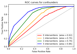
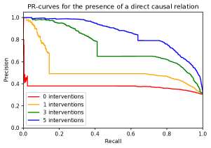
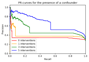
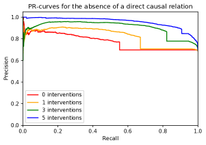
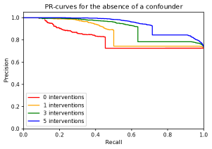
Figure 6: ROC curves (top) and PR curves (center, bottom) for directed edges (left) and confounders (right), for different numbers of single-variable interventions. All results shown here use $\sigma$-separation.

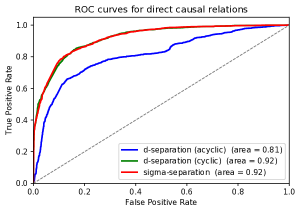
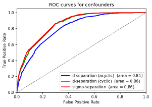
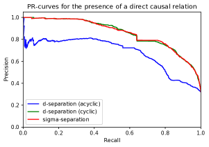
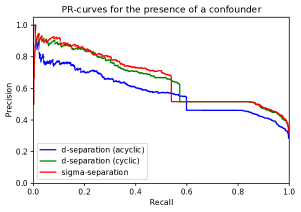
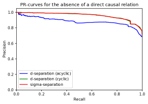
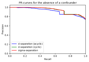
Figure 7: ROC curves (top) and PR curves (center, bottom) for directed edges (left) and confounders (right), for different encodings. All results shown here use observational and 5 interventional data sets.

References

- [1] F. Barthe, O. Guédon, S. Mendelson, and A. Naor. A probabilistic approach to the geometry of the -ball. Ann. Probab., 33(2):480–513, 2005.
- [2] V.I. Bogachev. Measure Theory. Vol. I, II. Springer, 2007.
- [3] S. Bongers, J. Peters, B. Schölkopf, and J. M. Mooij. Theoretical aspects of cyclic structural causal models. arXiv.org preprint, arXiv:1611.06221v2 [stat.ME], 2018.
- [4] T. Claassen and T. Heskes. Bayesian probabilities for constraint-based causal discovery. In IJCAI-13, pages 2992–2996, 2013.
- [5] T. Claassen, J.M. Mooij, and T. Heskes. Learning Sparse Causal Models is not NP-hard. In UAI-13, pages 172–181, 2013.
- [6] G. F. Cooper and E. Herskovits. A Bayesian method for the induction of probabilistic networks from data. Machine Learning, 9:309–347, 1992.
- [7] M. Drton, M. Eichler, and T. Richardson. Computing maximum likelihood estimates in recursive linear models with correlated errors. Journal of Machine Learning Research, 10:2329–2348, 2009.
- [8] R. Evans and T. Richardson. Maximum likelihood fitting of acyclic directed mixed graphs to binary data. In UAI-10, 2010.
- [9] R.J. Evans. Graphs for margins of Bayesian networks. Scand. J. Stat., 43(3):625–648, 2016.
- [10] R.J. Evans. Margins of discrete Bayesian networks. arXiv:1501.02103, pages 1–41, 2017. Submitted to Annals of Statistics.
- [11] R.J. Evans and T.S. Richardson. Markovian acyclic directed mixed graphs for discrete data. Ann. Statist., 42(4):1452–1482, 08 2014.
- [12] P. Forré and J. M. Mooij. Markov properties for graphical models with cycles and latent variables. arXiv:1710.08775, 2017.
- [13] M. Gebser, R. Kaminski, B. Kaufmann, and T. Schaub. Clingo = ASP + control: Extended report. Technical report, University of Potsdam, 2014. http://www.cs.uni-potsdam.de/wv/pdfformat/gekakasc14a.pdf.
- [14] D. Geiger and D. Heckerman. Learning Gaussian networks. In UAI-94, pages 235–243, 1994.
- [15] M. Gelfond. Answer sets. In Handbook of Knowledge Representation, pages 285–316. 2008.
- [16] I. Goodfellow, Y. Bengio, and A. Courville. Deep Learning. MIT Press, 2016.
- [17] D. Heckerman, C. Meek, and G. Cooper. A Bayesian approach to causal discovery. In C. Glymour and G. F. Cooper, editors, Computation, Causation, and Discovery, pages 141–166. MIT Press, 1999.
- [18] A. Hyttinen, F. Eberhardt, and P.O. Hoyer. Causal discovery for linear cyclic models. In Proceedings of the Fifth European Workshop on Probabilistic Graphical Models, 2010.
- [19] A. Hyttinen, F. Eberhardt, and M. Järvisalo. Constraint-based causal discovery: Conflict resolution with answer set programming. In UAI-14, pages 340–349, 2014.
- [20] V. Lifschitz. What is Answer Set Programming? In AAAI Conference on Artificial Intelligence, pages 1594–1597, 2008.
- [21] S. Magliacane, T. Claassen, and J.M. Mooij. Ancestral causal inference. In NIPS-16, pages 4466–4474. 2016.
- [22] C. Meek. Strong completeness and faithfulness in Bayesian networks. In UAI-95, pages 411–418, 1995.
- [23] J. M. Mooij, S. Magliacane, and T. Claassen. Joint causal inference from multiple contexts. arXiv.org preprint, https://arxiv.org/abs/1611.10351v3 [cs.LG], March 2018.
- [24] J. Pearl. Fusion, propagation and structuring in belief networks. Technical Report 3, UCLA Computer Science Department, 1986. Technical Report 850022 (R-42).
- [25] J. Pearl. Causality: Models, reasoning, and inference. Cambridge University Press, 2nd edition, 2009.
- [26] J. Peters, D. Janzing, and B. Schölkopf. Elements of Causal Inference: Foundation and Learning Algorithms. MIT press, 2017.
- [27] T. Richardson. A discovery algorithm for directed cyclic graphs. In UAI-96, pages 454–461. 1996.
- [28] T. Richardson. Markov properties for acyclic directed mixed graphs. Scand. J. Stat., 30(1):145–157, 2003.
- [29] T. Richardson and P. Spirtes. Automated discovery of linear feedback models. In C. Glymour and G. F. Cooper, editors, Computation, Causation, and Discovery, pages 253–304. MIT Press, 1999.
- [30] D. Rothenhäusler, C. Heinze, J. Peters, and N. Meinshausen. BACKSHIFT: Learning causal cyclic graphs from unknown shift interventions. In NIPS-15, pages 1513–1521. 2015.
- [31] P. Spirtes. Directed cyclic graphical representations of feedback models. In UAI-95, pages 491–499, 1995.
- [32] P. Spirtes, C. Glymour, and R. Scheines. Causation, Prediction, and Search. MIT press, 2000.
- [33] T.S. Verma and J. Pearl. Causal Networks: Semantics and Expressiveness. UAI-90, 4:69–76, 1990.
- [34] J. Zhang. On the completeness of orientation rules for causal discovery in the presence of latent confounders and selection bias. Artificial Intelligence, 172(16-17):1873–1896, 2008.