Non-Oberbeck-Boussinesq zonal flow generation

Abstract

Novel mechanisms for zonal flow (ZF) generation for both large relative density fluctuations and background density gradients are presented. In this non-Oberbeck-Boussinesq (NOB) regime ZFs are driven by the Favre stress, the large fluctuation extension of the Reynolds stress, and by background density gradient and radial particle flux dominated terms. Simulations of a nonlinear full-F gyro-fluid model confirm the predicted mechanism for radial ZF propagation and show the significance of the NOB ZF terms for either large relative density fluctuation levels or steep background density gradients.

I Introduction

Self-organization from turbulent to coherent states is a ubiquitous process in fluids. In particular, much interest and effort has been drawn to the formation of zonal flows (ZFs) Diamond et al. (2005); Fujisawa (2009); Gürcan and Diamond (2015). These coherent flows arise in atmospheres, in the form of banded cloud structures on Jupiter Heimpel, Aurnou, and Wicht (2005), Saturn’s north-polar hexagon Baines et al. (2009) or mid-latitude westerlies on earth and in the ocean as stationary jets Maximenko, Bang, and Sasaki (2005). In magnetized fusion plasmas ZFs are key players for the reduction of the radial transport of particles and heat and for the transition to improved confinement regimes in tokamaks Burrell (1997); Terry (2000); Hillesheim et al. (2016); Tynan et al. (2016); Schmitz (2017); Cziegler et al. (2017).

Reynolds stress is quintessential for ZF generation in all fluids Diamond and Kim (1991); Xu et al. (2000); Diamond et al. (2005); Fujisawa (2009); Müller et al. (2011); Xu et al. (2011); Yan et al. (2014); Gürcan and Diamond (2015), but in magnetized plasmas also other stresses like the Maxwell Craddock and Diamond (1991); Scott (2005) or the diamagnetic stress Smolyakov, Diamond, and Medvedev (2000); Madsen et al. (2017) can become significant. Virtually all of the work on ZF theory so far rely on $\delta{f}$ models Diamond and Kim (1991); Diamond et al. (2005); Guo and Diamond (2016), which invoke the so called Oberbeck-Boussinesq (or thin layer) approximation Oberbeck (1879); Boussinesq (1903). However, the latter breaks down, if the background density varies over more than one order of magnitude or if the relative density fluctuations exceed roughly $10$ percent. This for example prevails in the edge of tokamak fusion plasmas, where experimental measurements typically feature relative density fluctuation levels around the order $0.1$ in the edge and up to unity at the last closed flux surface Surko and Slusher (1983); Liewer (1985); Ritz et al. (1987); Fonck et al. (1993); Endler et al. (1995); McKee et al. (2001); Zweben et al. (2007, 2015); Gao et al. (2015). Moreover, typical edge background density gradient (e-folding) lengths reach from $50\rho_{s0}$ in low-confinement to $10\rho_{s0}$ in high-confinement tokamak plasmas Shao et al. (2016); Kobayashi et al. (2016). Here, $\rho_{s0}:=\sqrt{T_{e0}m_{i}}/(eB_{0})$ is the drift scale with reference electron temperature $T_{e0}$, ion particle charge $e$, ion mass $m_{i}$ and reference magnetic field $B_{0}$.

Non-Oberbeck-Boussinesq (NOB) effects on ZF generation are an unresolved issue. However, theoretical and experimental studies of poloidal ZFs in the edge of fusion plasmas indicate that unknown mechanisms beyond the Reynolds stress exist Kobayashi et al. (2013) and that steep background density gradients and large relative density fluctuations affect the poloidal ZF dynamics Müller et al. (2011); Windisch et al. (2011); Wang, Wen, and Diamond (2016). Moreover, the importance of large relative density fluctuations for toroidal momentum transport, as suggested by theoretical estimates in the strong and weak turbulence regime Wang, Wen, and Diamond (2015); Kosuga et al. (2017) and experimental measurements in the TORPEX and PANTA device Labit et al. (2011); Inagaki et al. (2016), point towards a similar significance for poloidal momentum transport.

In the following we generalize the theory of ZFs to NOB effects. To this end, we decompose the density and electric potential of a full-F gyro-fluid model of a magnetized plasma Madsen (2013) with the help of a density weighted Favre average Favre (1965). This well known decomposition strategy in compressible fluid dynamics (see e.g. Wilcox (2000)) is here for the first time introduced to plasma physics and enables us to disentangle the density fluctuations from the ZF dynamics, while retaining the relevant physical effects. As a result, we identify novel agents in the poloidal ZF dynamics, which become significant for high relative density fluctuations or steep background density gradients. We confirm the herein proposed NOB mechanism for radial advection of ZFs with the help of numerical simulations of a fully nonlinear model for drift wave-ZF dynamics. The exploited model is based on the specified extension of the Hasegawa-Wakatani model to the full-F framework. Additionally, we show how the ZF dynamics is distributed among the proposed NOB actors and provide scalings with collisionality, reference background density gradient length and the maximum of the relative density fluctuation amplitude.

II ZF theory

II.1 $\delta{f}$ formalism

We start our discussion with a short re-derivation of the conventional ZF equation and Reynolds stress from a cold ion $\delta{f}$ gyro-fluid model, which couples small relative density fluctuations to the electric potential via ${\mathbf{E}}\times{\mathbf{B}}$ advection and linear polarization Dorland and Hammett (1993); Beer and Hammett (1996); Scott (2010)

$$\frac{\partial}{\partial t}\delta{n}+{\mathbf{\nabla}}\cdot\left(\delta{n}{\mathbf{u}}_{E}\right)+\frac{1}{L_{n}B_{0}}\frac{\partial}{\partial y}\phi=\Lambda_{\delta},$$ (1a)

$$\frac{\partial}{\partial t}\delta{N}+{\mathbf{\nabla}}\cdot\left(\delta{N}{\mathbf{u}}_{E}\right)+\frac{1}{L_{n}B_{0}}\frac{\partial}{\partial y}\phi=0,$$ (1b)

$${\mathbf{\nabla}}\cdot\left(\frac{1}{\Omega_{0}}\frac{{\mathbf{\nabla}}_{\perp}\phi}{B_{0}}\right)=\delta{n}-\delta{N}.$$ (1c)

Here, $\delta{n}:=n/n_{G}-1$ is the relative electron density fluctuation, $\delta{N}:=N/n_{G}-1$ is the relative ion gyro-center density fluctuation, $\phi$ is the electric potential and $\Omega_{0}:=eB_{0}/m_{i}$ is the ion gyro-frequency. The reference background density $n_{G}(x)$ refers to a constant reference background gradient length $L_{n}:=-1/\partial_{x}\ln{(n_{G}/n_{0})}$ with constant reference density $n_{0}$. For the sake of simplicity the magnetic field $B=B_{0}$ is assumed constant and the unit vector in the magnetic field direction is $\hat{{\mathbf{b}}}:={\mathbf{B}}/B_{0}={\mathbf{\hat{e}}}_{z}$. The perpendicular gradient and the ${\mathbf{E}}\times{\mathbf{B}}$ drift velocity are defined by ${\mathbf{\nabla}}_{\perp}:=-\hat{{\mathbf{b}}}\times(\hat{{\mathbf{b}}}\times{\mathbf{\nabla}})$ and ${\mathbf{u}}_{E}:=\hat{{\mathbf{b}}}\times{\mathbf{\nabla}}\phi/B_{0}$, respectively. The term $\Lambda_{\delta}$ denotes a closure for the parallel dynamics, which is discussed later in more detail. Taking the time derivative over the polarization equation (1c) yields the $\delta{f}$ drift-fluid vorticity density equation

$$\frac{\partial}{\partial t}\mathcal{W}_{\delta}+{\mathbf{\nabla}}\cdot\left(\mathcal{W}_{\delta}{\mathbf{u}}_{E}\right)=\Omega_{0}n_{0}\Lambda_{\delta},$$ (2)

with the linear ${\mathbf{E}}\times{\mathbf{B}}$ vorticity density $\mathcal{W}_{\delta}:=n_{0}{\mathbf{\nabla}}_{\perp}^{2}\phi/B_{0}=\hat{{\mathbf{b}}}\cdot{\mathbf{\nabla}}\times\left(n_{0}{\mathbf{u}}_{E}\right)$. Now we apply the average over the “poloidal” y coordinate $\langle h\rangle:=L_{y}^{-1}\int_{0}^{L_{y}}dy\hskip 2.84526pth$ to Eq. (2), which is the 2D equivalent of a flux surface average. Reynolds decomposition $h=\langle h\rangle+\widetilde{h}$ and integration over the “radial” coordinate $x$ result in the $\delta{f}$ evolution equation for poloidal ZFs Diamond and Kim (1991)

$$\frac{\partial}{\partial t}\langle u_{y}\rangle= -\frac{\partial}{\partial x}\langle\widetilde{u_{x}}\widetilde{u_{y}}\rangle+\Omega_{0}\int_{x_{0}}^{x}dx\langle\Lambda_{\delta}\rangle.$$ (3)

Here, we introduced $u_{x}:=-\partial_{y}\phi/B_{0}$, $u_{y}:=\partial_{x}\phi/B_{0}$ and the anticipated Reynolds stress $\mathcal{R}:=\langle\widetilde{u_{x}}\widetilde{u_{y}}\rangle$ Reynolds (1895), where $\langle u_{x}u_{y}\rangle=\langle u_{x}\rangle\langle u_{y}\rangle+\langle\widetilde{u_{x}}\widetilde{u_{y}}\rangle$ and $\langle u_{x}\rangle=0$ was used. In passing we note that we assume that radial boundary conditions give rise to no additional terms in Eq. (3) and for the remainder of this letter.

II.2 Full-F formalism

In full-F theory the splitting of the gyro-fluid moment variables into fluctuating and background parts is avoided and the quasi-neutrality constraint for electrons and ions is rendered by the nonlinear polarization equation Madsen (2013). The cold ion full-F gyro-fluid model Wiesenberger, Madsen, and Kendl (2014); Held et al. (2016)

$$\frac{\partial}{\partial t}n+{\mathbf{\nabla}}\cdot\left(n{\mathbf{u}}_{E}\right)=\Lambda,$$ (4a)

$$\frac{\partial}{\partial t}N+{\mathbf{\nabla}}\cdot\left(N{\mathbf{U}}_{E}\right)=0,$$ (4b)

$${\mathbf{\nabla}}\cdot\left(\frac{N}{\Omega_{0}}\frac{{\mathbf{\nabla}}_{\perp}\phi}{B_{0}}\right)=n-N,$$ (4c)

evolves the full electron density ${n}$ and ion gyro-center density $N$. In the gyro-center ${\mathbf{E}}\times{\mathbf{B}}$ drift velocity by ${\mathbf{U}}_{E}:={\mathbf{u}}_{E}+{\mathbf{U}}_{p}$ the ponderomotive correction ${\mathbf{U}}_{p}:=-\hat{{\mathbf{b}}}\times{\mathbf{\nabla}}{\mathbf{u}}_{E}^{2}/(2\Omega_{0})$ appears. Both, the latter ponderomotive correction and the polarization charge nonlinearity on the left hand side of Eq. (4c) are crucial for energetic consistency and an exact momentum conservation law Scott and Smirnov (2010). We refer to the parallel closure term $\Lambda$ later on. In the long wavelength limit we can again reformulate Eqs. (4b) and (4c) into a drift-fluid vorticity density equation

$$\frac{\partial}{\partial t}\mathcal{W}+{\mathbf{\nabla}}\cdot\left(\mathcal{W}{\mathbf{u}}_{E}\right)-\Omega_{0}{\mathbf{\nabla}}\cdot\left(n{\mathbf{U}}_{p}\right)=\Omega_{0}\Lambda,$$ (5)

where the nonlinear ${\mathbf{E}}\times{\mathbf{B}}$ vorticity density is given by $\mathcal{W}:={\mathbf{\nabla}}\cdot\left(n{\mathbf{\nabla}}_{\perp}\phi/B_{0}\right)=\hat{{\mathbf{b}}}\cdot{\mathbf{\nabla}}\times\left(n{\mathbf{u}}_{E}\right)$. As above, we obtain the averaged poloidal momentum equation  Gürcan et al. (2007); Shurygin (2012); Wang, Wen, and Diamond (2016)

$$\frac{\partial}{\partial t}\langle nu_{y}\rangle= -\frac{\partial}{\partial x}\left(\langle n\rangle\mathcal{R}+\langle\widetilde{n}\widetilde{u_{x}}\rangle\langle u_{y}\rangle+\langle\widetilde{n}\widetilde{u_{x}}\widetilde{u_{y}}\rangle\right)$$

$$+\Omega_{0}\int_{x_{0}}^{x}dx\langle\Lambda\rangle.$$ (6)

The divergence of the full-F stress drive terms of Eq. (II.2) is related to the averaged radial flux of vorticity density minus the ponderomotive correction via the full-F Taylor identity

$$\langle\widetilde{u_{x}}\widetilde{\mathcal{W}}\rangle= \frac{\partial}{\partial x}\big{[}\langle n\rangle\mathcal{R}+\langle\widetilde{n}\widetilde{u_{x}}\rangle\langle u_{y}\rangle+\langle\widetilde{n}\widetilde{u_{x}}\widetilde{u_{y}}\rangle\big{]}$$

$$+\Omega_{0}\langle\widetilde{U_{p,x}}\widetilde{n}\rangle.$$ (7)

The interpretation of Eq. (II.2) is problematic since (i) absolute density fluctuations $\widetilde{n}$ arise instead of relative density fluctuations $\widetilde{n}/\langle n\rangle$, (ii) the time evolution of the averaged poloidal momentum $\langle nu_{y}\rangle$ is given in terms of the averaged poloidal velocity $\langle u_{y}\rangle$ and (iii) background density gradient $\partial_{x}\ln{\langle n\rangle}$ effects are not obvious. Despite these obstacles Eq. (II.2) has been recently used to show that the second term, occasionally misinterpreted as advective, and the cubic term can be comparable to the Reynolds stress related drive $\partial_{x}(\langle n\rangle\mathcal{R})$ Müller et al. (2011); Windisch et al. (2011); Wang, Wen, and Diamond (2016).

Thus, we go a step further and utilize a density weighted Favre decomposition instead of the Reynolds decomposition according to $h:=\left[\left[h\right]\right]+\widehat{h}$ and $\left[\left[h\right]\right]:=\langle nh\rangle/\langle n\rangle$ Favre (1965). Note that the Favre decomposition reduces to the Reynolds decomposition if the density $n$ is only a function of $x$. Now we combine the poloidal average of Eq. (4a) divided by $\langle n\rangle$

$$\frac{\partial}{\partial t}\ln{\langle n\rangle}= -\frac{\partial}{\partial x}\left[\left[u_{x}\right]\right]-\left[\left[u_{x}\right]\right]\frac{\partial}{\partial x}\ln{\langle n\rangle}$$

$$+\frac{\langle\Lambda\rangle}{\langle n\rangle}$$ (8)

with Eq. (II.2) divided by $\langle n\rangle$ to obtain a ZF evolution equation for the Favre averaged poloidal velocity

$$\frac{\partial}{\partial t}\left[\left[u_{y}\right]\right]= -\frac{\partial}{\partial x}\left[\left[\widehat{u_{x}}\widehat{u_{y}}\right]\right]-\left[\left[u_{x}\right]\right]\frac{\partial}{\partial x}\left[\left[u_{y}\right]\right]$$

$$-\left[\left[\widehat{u_{x}}\widehat{u_{y}}\right]\right]\frac{\partial}{\partial x}\ln{\langle n\rangle}$$

$$-\left[\left[u_{y}\right]\right]\frac{\langle\Lambda\rangle}{\langle n\rangle}+\frac{\Omega_{0}}{\langle n\rangle}\int_{x_{0}}^{x}dx\langle\Lambda\rangle,$$ (9)

where we used $\left[\left[u_{x}u_{y}\right]\right]=\left[\left[u_{x}\right]\right]\left[\left[u_{y}\right]\right]+\left[\left[\widehat{u_{x}}\widehat{u_{y}}\right]\right]$. The Favre stress $\mathcal{F}:=\left[\left[\widehat{u_{x}}\widehat{u_{y}}\right]\right]$ can be rewritten into

$$\mathcal{F}=\mathcal{R}-\left[\left[\widetilde{u_{x}}\right]\right]\left[\left[\widetilde{u_{y}}\right]\right]+\langle\widetilde{n}\widetilde{u_{x}}\widetilde{u_{y}}\rangle/\langle n\rangle.$$ (10)

Consequently, the first term $-\partial_{x}\mathcal{F}$ on the right hand side of Eq. (II.2) is the superposition of the conventional Reynolds stress drive $T_{1}:=-\partial_{x}\mathcal{R}$, the quadruple fluctuation term $T_{2}:=\partial_{x}\left(\left[\left[\widetilde{u_{x}}\right]\right]\left[\left[\widetilde{u_{y}}\right]\right]\right)$ and the triple fluctuation drive $T_{3}:=-\partial_{x}\left(\langle\widetilde{n}\widetilde{u_{x}}\widetilde{u_{y}}\rangle/\langle n\rangle\right)$. The novel second term on the right hand side of Eq. (II.2) represents radial advection of poloidal ZFs $\left[\left[u_{y}\right]\right]$. Its direction depends on the sign of the averaged radial particle flux $\langle\Gamma_{x}\rangle:=\langle n\rangle\left[\left[u_{x}\right]\right]$, which is typically positive, so that $T_{4}$ describes an outward pinch of ZFs. The novel third term $T_{5}:=\mathcal{F}/L_{\langle n\rangle}$ on the right hand side of Eq. (II.2) is proportional to the inverse of the background density gradient length $1/L_{\langle n\rangle}:=-\partial_{x}\ln{\langle n\rangle}$. This term is large for small reference background density gradient lengths $L_{n}$, or has large radially localized values if the density profile $\langle n\rangle$ develops into a staircase like pattern Dif-Pradalier et al. (2015). In contrast to the Favre stress drive $-\partial_{x}\mathcal{F}$, the background density gradient drive $T_{5}$ contributes to the ZF generation even if the Favre stress is radially homogeneous $\partial_{x}\mathcal{F}=0$. Remarkably, the background density gradient drive remains finite in the small relative density fluctuation limit, where the density $n$ is only a function of $x$ and the Favre stress $\mathcal{F}$ resembles the conventional Reynolds stress $\mathcal{R}$.

In order to interpret the dynamics of the background density gradient drive $T_{5}$ let us assume for a moment that the turbulent viscosity hypothesis $\mathcal{F}:=-\nu_{T}(x)\frac{\partial}{\partial x}\left[\left[u_{y}\right]\right]$ holds Diamond and Kim (1991); Pope (2000). In this case Eq. (II.2) reduces to a simple advection-diffusion equation for ZFs

$$\frac{\partial}{\partial t}\left[\left[u_{y}\right]\right]= -\left(\left[\left[u_{x}\right]\right]+V\right)\frac{\partial}{\partial x}\left[\left[u_{y}\right]\right]$$

$$+\frac{\partial}{\partial x}\left(\nu_{T}\frac{\partial}{\partial x}\left[\left[u_{y}\right]\right]\right)-\left[\left[u_{y}\right]\right]\frac{\langle\Lambda\rangle}{\langle n\rangle}$$

$$+\frac{\Omega_{0}}{\langle n\rangle}\int_{x_{0}}^{x}dx\langle\Lambda\rangle,$$ (11)

where the background density gradient pinch velocity $V:=\nu_{T}/L_{\langle n\rangle}$ appears now in addition to the radial outward pinch velocity $\left[\left[u_{x}\right]\right]$. The direction of the additional pinch depends on the sign of the turbulent viscosity $\nu_{T}$.

Finally, we extend the theory for energy transfer inside the kinetic ${\mathbf{E}}\times{\mathbf{B}}$ energy $E(t):=m_{i}\int dA\langle n{\mathbf{u}}_{E}^{2}\rangle/2$ to the full-F formalism. Here, the Favre decomposition $E=E_{0}+E_{1}$ is pivotal to derive the conservation laws for the zonal (or mean) $E_{0}(t):=m_{i}\int dA\langle n\rangle\left[\left[u_{y}\right]\right]^{2}/2$ and turbulent part $E_{1}(t):=m_{i}\int dA\langle n\rangle\widehat{{\mathbf{u}}}_{E}^{2}/2$ of the kinetic ${\mathbf{E}}\times{\mathbf{B}}$ energy and supersedes the Reynolds decomposition in the $\delta{f}$ formalism Scott (2005); Madsen et al. (2017). With the help of Eqs. (II.2) and  (II.2) we obtain the conservation laws for the zonal and turbulent kinetic ${\mathbf{E}}\times{\mathbf{B}}$ energy

$$\frac{\partial}{\partial t}E_{0}= \int dA\hskip 2.84526ptm_{i}\Big{(}\langle n\rangle\mathcal{F}\frac{\partial}{\partial x}\left[\left[u_{y}\right]\right]-\frac{\left[\left[u_{y}\right]\right]^{2}}{2}\langle\Lambda\rangle$$ (12a)

$$+\Omega_{0}\left[\left[u_{y}\right]\right]\int_{x_{0}}^{x}dx\langle\Lambda\rangle\Big{)},$$

$$\qquad\frac{\partial}{\partial t}E_{1}= \int dA\hskip 2.84526ptm_{i}\Big{(}-\langle n\rangle\mathcal{F}\frac{\partial}{\partial x}\left[\left[u_{y}\right]\right]+\frac{\left[\left[u_{y}\right]\right]^{2}}{2}\langle\Lambda\rangle$$ (12b)

$$-\Omega_{0}\left[\left[u_{y}\right]\right]\int_{x_{0}}^{x}dx\langle\Lambda\rangle-\frac{e}{m_{i}}\langle\phi\Lambda\rangle\Big{)}.$$

This unveils that the Favre stress term $\langle n\rangle\mathcal{F}\frac{\partial}{\partial x}\left[\left[u_{y}\right]\right]$ is the central mechanism for energy transfer between the zonal and turbulent kinetic ${\mathbf{E}}\times{\mathbf{B}}$ energy. As a consequence, density fluctuations (cf. Eq. (10)) manifest as an additional transfer channel in the full-F formalism.

III Parallel closures

Self-sustained drift wave turbulence is maintained by the non-adiabatic parallel coupling of the relative density fluctuations and the electric potential, which can arise due to various mechanisms. Here, we exemplarily consider resistive drift wave turbulence, which arises due to resistive friction between electrons and ions along the magnetic field line. This mechanism enters the 2D gyro-fluid models via the parallel closure terms ($\Lambda_{\delta}$ or $\Lambda$) of the Hasegawa-Wakatani (HW) type as summarized in Table 1.

Table 1: HW closures for $\delta{f}$ and full-F models.

	ordinary HW	modified HW
$\Lambda_{\delta}/(\alpha_{\delta}\Omega_{0})$	$e\phi/T_{e0}-\delta{n}$ Hasegawa and Wakatani (1983); Wakatani and Hasegawa (1984); Hasegawa and Wakatani (1987)	$e\widetilde{\phi}/T_{e0}-\widetilde{\delta{n}}$ Numata, Ball, and Dewar (2007)
${\Lambda}/(\alpha n_{0}\Omega_{0})$	$e\phi/T_{e0}-\ln\left(n/\langle n\rangle\right)$	$e\widetilde{\phi}/T_{e0}-\widetilde{\ln\left(n\right)}$

Here, we introduced the full-F adiabaticity parameter $\alpha:=T_{e0}k_{\parallel}^{2}/(\eta_{\parallel}e^{2}n_{0}\Omega_{0})$ with parallel wavenumber $k_{\parallel}$ and parallel Spitzer resistivity $\eta_{\parallel}:=0.51m_{e}\nu_{e}/(ne^{2})$ Spitzer (1956); Lingam et al. (2017). In the electron collision frequency $\nu_{e}$ the Coulomb logarithm is treated as a constant so that $\eta_{\parallel}$ has no explicit dependence on $n$. As opposed to this in $\delta{f}$ models the density dependence in the collision frequency $\nu_{e}(n)\approx\nu_{e0}$ is completely neglected so that $\alpha_{\delta}:=T_{e0}k_{\parallel}^{2}/(0.51m_{e}\nu_{e0}\Omega_{0})$ reduces to a parameter. Only then, the poloidal variations of the adiabaticity parameters vanish ($\widetilde{\alpha_{\delta}}=\widetilde{\alpha}=0$), and the full-F and $\delta{f}$ closures coincide in the limit of $\langle n\rangle\approx n_{G}$ and $\delta{n}\ll 1$.

IV Simulations

We use the open source library Feltor Wiesenberger and Held (2018) to numerically solve the full-F gyro-fluid Eqs.  (4) with the modified HW parallel closure of Table 1. Numerical stability is ensured by adding hyperdiffusive terms of second order $-\nu{\mathbf{\nabla}}_{\perp}^{4}n$ and $-\nu{\mathbf{\nabla}}_{\perp}^{4}N$ to the right hand side of Eqs. (4a) and (4b). Moreover, we append the right hand side of Eqs (4a) and (4b) by a density source of the form $\omega_{S}z\hskip 1.42262pt\Theta\left(z\right)$ with $z:=g(x)\left(n_{G}-\langle n\rangle\right)$ to maintain the initial profile in a small region $x\in\left[0,x_{b}\right]$. Here, we defined the Heaviside function $\Theta(z)$ and $g(x):=\left[1-\tanh{(x-x_{b})/\sigma_{b}}\right]/2$. The corresponding parameters are fixed to $\nu=5\times 10^{-4}c_{s0}\rho_{s0}^{3}$, $\omega_{S}=0.1\Omega_{0}$, $x_{b}=0.1L_{x}$ and $\sigma_{b}=0.5\rho_{s0}$ with cold ion sound speed $c_{s0}:=\rho_{s0}\Omega_{0}$. The box with size $L_{x}=L_{y}=128\rho_{s0}$ is resolved by a discontinuous Galerkin discretization with $P=3$ polynomial coefficients and at least $N_{x}=N_{y}=256$ equidistant grid cells. The initial (gyro-center) density fields $n({\mathbf{x}},0)=N({\mathbf{x}},0)=n_{G}(x)\left(1+\delta{n}_{0}({\mathbf{x}})\right)$ consist of the reference background density profile $n_{G}$, which is perturbed by a turbulent bath $\delta{n}_{0}({\mathbf{x}})$.

NOB effects on drift wave-ZF dynamics, as it is described by Eqs. (II.2) and (II.2) with $\langle\Lambda\rangle=0$, are in this setup studied by varying the adiabaticity parameter (or inverse collisionality) $\alpha$ and the reference background gradient length $L_{n}$. In Fig. 1 we show that $L_{n}$ crucially determines the time evolution of ZFs in the high collisionality regime with $\alpha=0.0005$. While stationary ZFs emerge for $L_{n}=128\rho_{s0}$, a radial outward pinch of ZFs occurs for a four times smaller reference background density gradient length $L_{n}=32\rho_{s0}$.

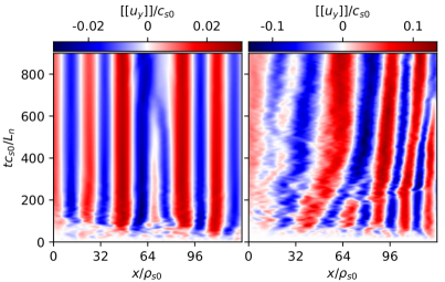
Figure 1: The spatio-temporal ZF evolution of the Favre averaged poloidal velocity $\left[\left[u_{y}\right]\right]$ is shown for two different reference density gradient lengths $L_{n}=\left\{128,32\right\}\rho_{s0}$ (left,right) in the high collisionality regime ($\alpha=0.0005$). Radial outward ZF advection occurs in the steep gradient regime (right).

In this steep gradient and high collisionality regime the ZF signature is no longer solely determined by the conventional Reynolds stress drive, which is illustrated in Fig. 2. The Reynolds stress drive $T_{1}$ is here comparable to the radial advection term $T_{4}$, which explains the observed radial outward propagation of ZFs in Fig. 1.

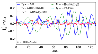
Figure 2: The radial profile of the terms of the right hand side of Eq. (II.2) for $\alpha=0.0005$ and $L_{n}=32\rho_{s0}$. The ZF signature of the radial advection term $T_{4}$ is comparable to the Reynolds stress $T_{1}$.

In the following the parametric dependence of each term $T_{i}$ on the right hand side of Eq. (II.2) is investigated. To this end, the contribution of each term $T_{i}$ on ZF evolution is measured by taking the $L^{2}$ norm, denoted by $\big{\|}h\big{\|}_{2}$, of the time integrated contribution. Following this, we propose a measure of the relative ZF contribution

$$M_{i} :=\frac{\big{\|}\int_{0}^{t_{1}}dt\hskip 1.42262ptT_{i}\big{\|}_{2}}{\sum_{j=1}^{5}\big{\|}\int_{0}^{t_{1}}dt\hskip 1.42262ptT_{j}\big{\|}_{2}}.$$ (13)

In Fig. 3a we show that the relative contribution $M_{i}$ of the NOB ZF terms ($T_{2},\dots,T_{5}$) decreases with the reference background density gradient length $L_{n}$ in the high collisionality regime ($\alpha=0.0005$). The summed up relative contribution of the NOB ZF terms exceeds the one of the conventional Reynolds stress for $L_{n}=32\rho_{s0}$. For steep reference background density gradients the radial advection term $T_{4}$ exhibits the largest relative contribution to the ZF dynamics of all the NOB terms.

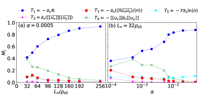
Figure 3: (a) The NOB ZF terms decrease with the reference background gradient length $L_{n}$ in the high collisionality regime ($\alpha=0.0005$). (b) For a fixed $L_{n}=32\rho_{s0}$ all the NOB ZF terms significantly contribute to the ZF dynamics in the high collisionality regime. As opposed to this, only the background density gradient drive $T_{5}$ remains alongside the Reynolds stress drive $T_{1}$ in the small collisionality regime.

In Fig. 3b the dependence of the relative importance of each term on the adiabaticity parameter $\alpha$ is depicted for a fixed reference background density gradient length $L_{n}=32\rho_{s0}$. While the conventional Reynolds stress term is again the dominating ZF contributor in particular for small collisionalities, all the NOB terms, except the background density gradient drive $T_{5}$, gain in importance for higher collisionalities. Interestingly, in the small collisionality regime ($\alpha\geq 0.01$) the background density gradient drive $T_{5}$ exceeds all the remaining NOB actors. The quadruple fluctuation drive $T_{2}$ is for all studied parameters the smallest contributor to the ZF dynamics.

The dependence of the ZF terms on the time averaged maximum of the relative density fluctuation level $\langle\big{\|}\widetilde{n}/\langle n\rangle\big{\|}_{\infty}\rangle_{t}$ is shown in Fig. 4. Here, we denote the time average by $\langle h\rangle_{t}$ and compute the maximum with the help of the supremum norm $\big{\|}h\big{\|}_{\infty}$. In Fig. 4 the conventional Reynolds stress drive $T_{1}$ contribution weakens with increasing relative density fluctuation level. The radial advection term $T_{4}$ and the triple fluctuation drive $T_{3}$ are the dominating NOB ZF contributors for high relative density fluctuations, while the background density gradient drive $T_{5}$ can be relevant likewise for small relative density fluctuations.

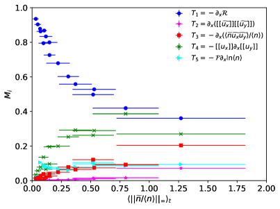
Figure 4: The relative contributions of the NOB ZF terms increase with the relative density fluctuation amplitude. In particular they can amount to roughly two thirds of the ZF dynamics.

V Conclusion

We have generalized the ZF equation (3) to account for NOB effects in Eq. (II.2). Most importantly, the former Reynolds stress $\mathcal{R}$ is replaced by the Favre stress $\mathcal{F}$, which adds to its predecessor in case of high relative density fluctuations. The latter is accompanied by two new agents in the NOB ZF Eq. (II.2). The first of these radially advects ZFs by the Favre averaged radial drift velocity, which is proportional to the averaged radial particle flux. The second term scales inversely with the background density gradient length and affects the ZF dynamics even if the relative density fluctuations are small or if the Favre stress is radially homogeneous. Thus, this term may be of significance in or during the formation of radial transport barriers, where steep density profiles form with strongly reduced radial particle transport.

Additionally we extended the ordinary and modified HW model to the full-F theory. We simulated the full-F gyro-fluid model with the modified HW closure to numerically corroborate our theoretical results. The simulations successfully reproduced the predicted radial advection of ZFs, which appeared for small reference background density gradient lengths and large averaged radial particle flux. Moreover, our numerical parameter study showed that the NOB ZF drives can be comparable to the Reynolds stress drive in the herein scanned parameter range. In particular the deviation between the Reynolds and Favre stress drive increases with the relative density fluctuation amplitude, collisionality and inversely with the reference background density gradient length. This deviation is mainly reasoned in the triple fluctuation drive. Its importance in steep background density gradient regimes is in qualitative agreement with the theoretical estimate in the strong turbulence regime Wang, Wen, and Diamond (2016). A similar dependence as for the Favre stress drive is found for the radial ZF advection mechanism. For the background density gradient drive only a dependence on the reference background density gradient is observed.

The presented results strongly argue in favor of the development and application of full-F gyro-fluid or gyro-kinetic models for simulation of fusion edge plasma turbulence, and in general demonstrate exemplarily the relevance of NOB effects for ZF formation in fluids and plasmas with large fluctuations and inhomogeneities. The latter conditions prevail e.g. during the low- to high-confinement mode transition. Thus, a consistent full-F simulation approach of this phenomenon is crucial to allow for the herein presented NOB ZF mechanisms.

Finally, we emphasize that the relative error between the Favre and Reynolds average of the poloidal velocity, derived to $|\left[\left[\widetilde{u_{y}}\right]\right]/\langle u_{y}\rangle|$, is typically below a few percent. Thus, our proposed NOB ZF theory is also applicable to experimental measurements of the Reynolds averaged poloidal velocity $\langle u_{y}\rangle$.

VI Acknowledgements

This work was supported by the Austrian Science Fund (FWF) Y398. R. K. was supported with financial subvention from the Research Council of Norway under grant 240510/F20. The computational results presented have been achieved using the Vienna Scientific Cluster (VSC) and the EUROfusion High Performance Computer (Marconi-Fusion). This work has been carried out within the framework of the EUROfusion Consortium and has received funding from the Euratom research and training programme 2014–2018 under grant agreement No 633053. The views and opinions expressed herein do not necessarily reflect those of the European Commission.

References

- Diamond et al. (2005) P. H. Diamond, S.-I. Itoh, K. Itoh, and T. S. Hahm, Plasma Physics and Controlled Fusion 47, R35 (2005).
- Fujisawa (2009) A. Fujisawa, Nuclear Fusion 49, 013001 (2009).
- Gürcan and Diamond (2015) Ö. D. Gürcan and P. H. Diamond, Journal of Physics A: Mathematical and Theoretical 48, 293001 (2015).
- Heimpel, Aurnou, and Wicht (2005) M. Heimpel, J. Aurnou, and J. Wicht, Nature 438, 193 (2005).
- Baines et al. (2009) K. H. Baines, T. W. Momary, L. N. Fletcher, A. P. Showman, M. Roos-Serote, R. H. Brown, B. J. Buratti, R. N. Clark, and P. D. Nicholson, Planetary and Space Science 57, 1671 (2009).
- Maximenko, Bang, and Sasaki (2005) N. A. Maximenko, B. Bang, and H. Sasaki, Geophysical Research Letters 32, L12607 (2005).
- Burrell (1997) K. H. Burrell, Physics of Plasmas 4, 1499 (1997).
- Terry (2000) P. W. Terry, Rev. Mod. Phys. 72, 109 (2000).
- Hillesheim et al. (2016) J. C. Hillesheim, E. Delabie, H. Meyer, C. F. Maggi, L. Meneses, E. Poli, and J. Contributors (EUROfusion Consortium, JET, Culham Science Centre, Abingdon, Oxon OX14 3DB, United Kingdom), Phys. Rev. Lett. 116, 065002 (2016).
- Tynan et al. (2016) G. R. Tynan, I. Cziegler, P. H. Diamond, M. Malkov, A. Hubbard, J. W. Hughes, J. L. Terry, and J. H. Irby, Plasma Physics and Controlled Fusion 58, 044003 (2016).
- Schmitz (2017) L. Schmitz, Nuclear Fusion 57, 025003 (2017).
- Cziegler et al. (2017) I. Cziegler, A. E. Hubbard, J. W. Hughes, J. L. Terry, and G. R. Tynan, Phys. Rev. Lett. 118, 105003 (2017).
- Diamond and Kim (1991) P. H. Diamond and Y. Kim, Physics of Fluids B: Plasma Physics 3, 1626 (1991).
- Xu et al. (2000) Y. H. Xu, C. X. Yu, J. R. Luo, J. S. Mao, B. H. Liu, J. G. Li, B. N. Wan, and Y. X. Wan, Phys. Rev. Lett. 84, 3867 (2000).
- Müller et al. (2011) H. Müller, J. Adamek, R. Cavazzana, G. Conway, C. Fuchs, J. Gunn, A. Herrmann, J. Horaček, C. Ionita, A. Kallenbach, M. Kočan, M. Maraschek, C. Maszl, F. Mehlmann, B. Nold, M. Peterka, V. Rohde, J. Schweinzer, R. Schrittwieser, N. Vianello, E. Wolfrum, M. Zuin, and the ASDEX Upgrade Team, Nuclear Fusion 51, 073023 (2011).
- Xu et al. (2011) G. S. Xu, B. N. Wan, H. Q. Wang, H. Y. Guo, H. L. Zhao, A. D. Liu, V. Naulin, P. H. Diamond, G. R. Tynan, M. Xu, R. Chen, M. Jiang, P. Liu, N. Yan, W. Zhang, L. Wang, S. C. Liu, and S. Y. Ding, Phys. Rev. Lett. 107, 125001 (2011).
- Yan et al. (2014) Z. Yan, G. R. McKee, R. Fonck, P. Gohil, R. J. Groebner, and T. H. Osborne, Phys. Rev. Lett. 112, 125002 (2014).
- Craddock and Diamond (1991) G. G. Craddock and P. H. Diamond, Phys. Rev. Lett. 67, 1535 (1991).
- Scott (2005) B. D. Scott, New Journal of Physics 7, 92 (2005).
- Smolyakov, Diamond, and Medvedev (2000) A. I. Smolyakov, P. H. Diamond, and M. V. Medvedev, Physics of Plasmas 7, 3987 (2000).
- Madsen et al. (2017) J. Madsen, J. J. Rasmussen, V. Naulin, and A. H. Nielsen, Physics of Plasmas 24, 062309 (2017).
- Guo and Diamond (2016) Z. B. Guo and P. H. Diamond, Phys. Rev. Lett. 117, 125002 (2016).
- Oberbeck (1879) A. Oberbeck, Ann. Phys. Chem (Berlin) 7, 271 (1879).
- Boussinesq (1903) J. Boussinesq, Theorie Analytique De La Chaleur, Vol. 2 (Gauthier-Villars, Paris, 1903).
- Surko and Slusher (1983) C. M. Surko and R. E. Slusher, Science 221, 817 (1983).
- Liewer (1985) P. C. Liewer, Nuclear Fusion 25, 543 (1985).
- Ritz et al. (1987) C. Ritz, D. Brower, T. Rhodes, R. Bengtson, S. Levinson, N. L. Jr., W. Peebles, and E. Powers, Nuclear Fusion 27, 1125 (1987).
- Fonck et al. (1993) R. J. Fonck, G. Cosby, R. D. Durst, S. F. Paul, N. Bretz, S. Scott, E. Synakowski, and G. Taylor, Phys. Rev. Lett. 70, 3736 (1993).
- Endler et al. (1995) M. Endler, H. Niedermeyer, L. Giannone, E. Kolzhauer, A. Rudyj, G. Theimer, and N. Tsois, Nuclear Fusion 35, 1307 (1995).
- McKee et al. (2001) G. McKee, C. Petty, R. Waltz, C. Fenzi, R. Fonck, J. Kinsey, T. Luce, K. Burrell, D. Baker, E. Doyle, X. Garbet, R. Moyer, C. Rettig, T. Rhodes, D. Ross, G. Staebler, R. Sydora, and M. Wade, Nuclear Fusion 41, 1235 (2001).
- Zweben et al. (2007) S. J. Zweben, J. A. Boedo, O. Grulke, C. Hidalgo, B. LaBombard, R. J. Maqueda, P. Scarin, and J. L. Terry, Plasma Physics and Controlled Fusion 49, S1 (2007).
- Zweben et al. (2015) S. Zweben, W. Davis, S. Kaye, J. Myra, R. Bell, B. LeBlanc, R. Maqueda, T. Munsat, S. Sabbagh, Y. Sechrest, D. Stotler, and the NSTX Team, Nuclear Fusion 55, 093035 (2015).
- Gao et al. (2015) X. Gao, T. Zhang, X. Han, S. Zhang, D. Kong, H. Qu, Y. Wang, F. Wen, Z. Liu, and C. Huang, Nuclear Fusion 55, 083015 (2015).
- Shao et al. (2016) L. M. Shao, E. Wolfrum, F. Ryter, G. Birkenmeier, F. M. Laggner, E. Viezzer, R. Fischer, M. Willensdorfer, B. Kurzan, T. Lunt, and the ASDEX Upgrade Team, Plasma Physics and Controlled Fusion 58, 025004 (2016).
- Kobayashi et al. (2016) T. Kobayashi, K. Itoh, T. Ido, K. Kamiya, S.-I. Itoh, Y. Miura, Y. Nagashima, A. Fujisawa, S. Inagaki, K. I. amd, and K. Hoshino, Scientific Reports 6, 30720 (2016).
- Kobayashi et al. (2013) T. Kobayashi, K. Itoh, T. Ido, K. Kamiya, S.-I. Itoh, Y. Miura, Y. Nagashima, A. Fujisawa, S. Inagaki, K. Ida, and K. Hoshino, Phys. Rev. Lett. 111, 035002 (2013).
- Windisch et al. (2011) T. Windisch, O. Grulke, V. Naulin, and T. Klinger, Plasma Physics and Controlled Fusion 53, 124036 (2011).
- Wang, Wen, and Diamond (2016) L. Wang, T. Wen, and P. Diamond, Nuclear Fusion 56, 106017 (2016).
- Wang, Wen, and Diamond (2015) L. Wang, T. Wen, and P. H. Diamond, Physics of Plasmas 22, 052302 (2015).
- Kosuga et al. (2017) Y. Kosuga, S.-I. Itoh, P. H. Diamond, and K. Itoh, Phys. Rev. E 95, 031203 (2017).
- Labit et al. (2011) B. Labit, C. Theiler, A. Fasoli, I. Furno, and P. Ricci, Physics of Plasmas 18, 032308 (2011).
- Inagaki et al. (2016) S. Inagaki, T. Kobayashi, Y. Kosuga, S.-I. Itoh, T. Mitsuzono, Y. Nagashima, H. Arakawa, T. Yamada, Y. Miwa, N. Kasuya, et al., Scientific reports 6, 22189 (2016).
- Madsen (2013) J. Madsen, Physics of Plasmas 20, 072301 (2013).
- Favre (1965) A. Favre, Journal de Mecanique 4, 361 (1965).
- Wilcox (2000) D. C. Wilcox, Turbulence Modeling for CFD (DCW Industries, 2000).
- Dorland and Hammett (1993) W. Dorland and G. W. Hammett, Physics of Fluids B 5, 812 (1993).
- Beer and Hammett (1996) M. A. Beer and G. W. Hammett, Physics of Plasmas 3, 4046 (1996).
- Scott (2010) B. Scott, Physics of Plasmas 17, 102306 (2010).
- Reynolds (1895) O. Reynolds, Philosophical Transactions of the Royal Society of London. A 186, 123 (1895).
- Wiesenberger, Madsen, and Kendl (2014) M. Wiesenberger, J. Madsen, and A. Kendl, Phys. Plasmas 21, 092301 (2014).
- Held et al. (2016) M. Held, M. Wiesenberger, J. Madsen, and A. Kendl, Nuclear Fusion 56, 126005 (2016).
- Scott and Smirnov (2010) B. Scott and J. Smirnov, Physics of Plasmas 17, 112302 (2010).
- Gürcan et al. (2007) Ö. D. Gürcan, P. H. Diamond, T. S. Hahm, and R. Singh, Physics of Plasmas 14, 042306 (2007).
- Shurygin (2012) R. V. Shurygin, Plasma Physics Reports 38, 93 (2012).
- Dif-Pradalier et al. (2015) G. Dif-Pradalier, G. Hornung, P. Ghendrih, Y. Sarazin, F. Clairet, L. Vermare, P. H. Diamond, J. Abiteboul, T. Cartier-Michaud, C. Ehrlacher, D. Estève, X. Garbet, V. Grandgirard, O. D. Gürcan, P. Hennequin, Y. Kosuga, G. Latu, P. Maget, P. Morel, C. Norscini, R. Sabot, and A. Storelli, Phys. Rev. Lett. 114, 085004 (2015).
- Pope (2000) S. B. Pope, Turbulent flows (Cambridge University Press, 2000).