The influence of absorbing boundary conditions on the transition path times statistics
	Michele Caraglio∗a, Stefanie Putb, Enrico Carlona, Carlo Vanderzandea,b‡
	We derive an analytical expression for the transition path time (TPT) distribution for a one-dimensional particle crossing a parabolic barrier. The solution is expressed in terms of the eigenfunctions and eigenvalues of the associated Fokker-Planck equation. The particle performs an anomalous dynamics generated by a power-law memory kernel, which includes memoryless Markovian dynamics as a limiting case. Our result takes into account absorbing boundary conditions, extending existing results obtained for free boundaries. We show that TPT distributions obtained from numerical simulations are in excellent agreement with analytical results, while the typically employed free boundary conditions lead to a systematic overestimation of the barrier height. These findings may be useful in the analysis of experimental results on transition path times. A web tool to perform this analysis is freely available.

1 Introduction

Quite some attention has been devoted in the past years to the study of transition path times (TPT) ^{1, 2, 3, 4, 5, 6, 7, 8, 9, 10, 11, 12, 13, 14, 15, 16, 17, 18, 19, 20, 21}. In a barrier-crossing process, such as the folding of biomolecules ²², transition paths are parts of a stochastic trajectory corresponding to an actual crossing event. Biomolecular folding is usually described as a transition between two stable conformations (the folded and unfolded states) using stochastic dynamics of a reaction coordinate moving on a double well potential landscape (see Fig. 1). Typically, the system spends most of its time close to one of the two minima, while transitions have very short duration. Despite the technical challenges due to the time resolution needed for TPT measurement, several experiments of the past few years determined average TPT in nucleic acids and protein folding ^{5, 8, 11, 18, 21}. The full probability distribution function of TPT was also obtained ¹⁴.

Transition paths are defined as those trajectories originating at a point $x_{a}$ ($x_{b}$), say, at one side of the barrier and ending in $x_{b}$ ($x_{a}$) at the opposite side (Fig. 1), without recrossing $x_{a}$ ($x_{b}$). Technically, this corresponds to imposing absorbing boundary conditions $P(x_{a},t)=P(x_{b},t)=0$, where $P(x,t)$ is the probability distribution of the particle position at time $t$. Current stochastic models employed to obtain TPT distributions use a parabolic barrier ^{3, 17, 19, 20}. As dealing with absorbing boundaries is challenging, free boundary conditions are instead preferred ^{5, 17}. This is a valid approximation as long as barriers are high compared to the thermal energy $k_{B}T$, since for very high barriers boundaries recrossings are highly unlikely. However, recent experiments analyzing TPT distributions in nucleic acid folding ¹⁴ estimated a barrier height of $\approx k_{B}T/2$. This value was obtained by fitting the data to the analytical form of the TPT distribution of the free boundary case, but the use of this distribution for barriers of the order of $k_{B}T$ or smaller is questionable.

Fig.  1: Sketch of a typical energy landscape as a function of a reaction coordinate $x$. The system fluctuates between the two minima. Transition paths are the parts of the trajectory originating in $x_{a}$ ($x_{b}$) and ending in $x_{b}$ ($x_{a}$) without crossing the two boundaries.

The aim of this paper is to calculate the TPT distribution for a parabolic barrier imposing absorbing boundaries at the two end points of the trajectories. This is done for a stochastic system whose evolution is described by a generalized Langevin equation with a power-law memory kernel (which also includes the Markovian dynamics in a limiting case). Anomalous dynamics is ubiquitous in macromolecular systems as polymers, as it is known from many examples ^{23, 24, 25, 26, 27, 28, 29, 30}. The calculation of the TPT distribution consists in expanding the solution of the Fokker-Planck equation in an infinite series of eigenfunctions (confluent hypergeometric functions). For the numerical estimate this series is truncated at a sufficiently high order. The results are in excellent agreement with numerical integration of the Langevin dynamics. Finally, we developed a web tool performing the fit of TPT distributions and providing an estimate of barrier height and friction coefficient in the Markovian case.

2 Generalized Langevin Equation

The formalism and theory follow closely the work of Goychuk and Hänggi ³¹ who considered the case of the escape out of a cusped-shape parabolic potential. The starting point is the Generalized Langevin Equation for an overdamped particle in a parabolic potential barrier $V(x)=-kx^{2}/2$ (note that the sign is reversed compared to the escape problem discussed in Ref. ³¹):

$$\int_{0}^{t}K(t-\tau)\ \accentset{\mbox{.}}{x}(\tau)d\tau=kx(t)+\xi(t)\;,$$ (1)

where $K(t)$ is a memory kernel and $\xi(t)$ is a random force with zero average $\langle\xi(t)\rangle=0$ and correlation given by the fluctuation-dissipation theorem

$$\langle\xi(t_{1})\xi(t_{2})\rangle=k_{B}TK(t_{1}-t_{2})\;,$$ (2)

In this paper we will consider a power-law memory kernel

$$K(t)=\dfrac{\eta_{\alpha}\,|t|^{-\alpha}}{\Gamma(1-\alpha)}\;,\qquad(0<\alpha<1)\;;$$ (3)

with $\eta_{\alpha}=\gamma\,\Gamma(3-\alpha)$. The Markovian limit is obtained as $\alpha\to 1^{-}$ leading to $K(t_{1}-t_{2})=2\gamma\delta(t_{1}-t_{2})$, with $\gamma$ the friction coefficient.

For a parabolic potential (1) can be mapped onto the following Fokker-Planck equation ^{32, 33, 34, 35, 31}

$$\dfrac{\partial P(x,t)}{\partial t} = D(t)\dfrac{\partial}{\partial x}\left(e^{\,\beta kx^{2}/2}\dfrac{\partial}{\partial x}e^{-\beta kx^{2}/2}P(x,t)\right)\;,$$ (4)

where $\beta=1/k_{B}T$ and $P(x,t)$ is the probability density of finding the particle in position $x$ at time $t$. $D(t)$ is a time-dependent diffusion coefficient given by ³¹

$$D(t)=\dfrac{k_{B}T}{k}\dfrac{d}{dt}\ln\theta(t)=\dfrac{k_{B}T}{k}\dfrac{\accentset{\mbox{.}}{\theta}(t)}{\theta(t)}\;,$$ (5)

where

$$\theta(t)=E_{\alpha}\left[\dfrac{k}{\eta_{\alpha}}t^{\alpha}\right]\;,$$ (6)

with $E_{\alpha}(z)=\sum_{n=0}^{\infty}z^{n}/\Gamma(\alpha n+1)$ the Mittag-Leffler function. In the Markovian limit $\alpha=1$ one has $E_{\alpha}(z)=e^{z}$ and, as expected, the time independent Einstein relation, $D=k_{B}T/\gamma$, is recovered from (5).

We seek a solution of Eq. (4) in the form of a spectral expansion $P(x,t)=\exp(\beta kx^{2}/4)\sum_{n}c_{n}Y_{n}(x)\varphi_{n}(t)$. Separation of variables leads to the following equation for the position-dependent part

$$Y^{\prime\prime}_{n}(x)-\left(\frac{\beta k}{2}+\frac{\beta^{2}k^{2}x^{2}}{4}\right)Y_{n}(x)=\lambda_{n}Y_{n}(x)\>,$$ (7)

while for the time-dependent part

$$\accentset{\mbox{.}}{\varphi}_{n}(t)=\lambda_{n}D(t)\varphi_{n}(t)\;.$$ (8)

The solution of the latter can be easily deduced from (5)

$$\varphi_{n}(t)=[\theta(t)]^{s_{n}}\;,$$ (9)

where $s_{n}\equiv\frac{k_{B}T}{k}\lambda_{n}$. Also the solutions of Eq. (7) are well known ³⁶. They are either even or odd functions in $x$ and can be written as

$$Y_{n}(x)=\left\{\begin{array}[]{l}e^{-\beta kx^{2}/4}\,{{}_{1}}F_{1}\left(\dfrac{s_{n}}{2}+\dfrac{1}{2};\dfrac{1}{2};\dfrac{\beta kx^{2}}{2}\right)\qquad\text{n=0,2,4\ldots}\\ \\ \sqrt{\beta k}\,x\,e^{-\beta kx^{2}/4}\,{{}_{1}}F_{1}\left(\dfrac{s_{n}}{2}+1;\dfrac{3}{2};\dfrac{\beta kx^{2}}{2}\right)\qquad\text{n=1,3,5\ldots}\end{array}\right.$$ (10)

where $\,{}_{1}F_{1}(a;b;z)$ is the Kummer confluent hypergeometric function. The boundary conditions $Y_{n}(\pm x_{0})=0$ fix the allowed values of $s_{n}$. Figure 2 shows a plot of the first five even and odd $Y_{n}(x)$ for $x_{0}=1$, $\beta=1$ and $k=10$. The values of $s_{n}$ for the first $10$ levels are also shown.

We note that Eq. (7) is analogous to the Schrödinger equation for a one-dimensional harmonic oscillator. In the ordinary quantum case one seeks normalizable wavefunctions decaying sufficiently fast at $\pm\infty$, which leads to the following values $s_{n}=\lambda_{n}/\beta k=-n-1$. One can recognize in this the energy levels of the one-dimensional quantum oscillator. In the present case, imposing vanishing functions at some finite $x$, as $Y_{n}(\pm x_{0})=0$, leads to non-integer values for $s_{n}$. Note however (Fig. 2) that $s_{n}$ for the lowest level are close to the quantum oscillator values $s_{n}\approx-n-1$. This is because the lowest states are strongly localized, therefore imposing vanishing functions at infinity or at some finite $x_{0}$ leads to a similar spectrum. The larger is the barrier ($\beta kx_{0}^{2}/2$), the closer is the spectrum of $s_{n}$ to that of the quantum oscillator.

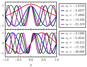
Fig.  2: Plot of normalized $Y_{n}(x)$ for $n=0,1,\ldots,9$ with $\beta=1$ and $k=10$. Absorbing boundary conditions are imposed in $x=\pm 1$, which leads to reported values of $s_{n}$ (obtained from numerical calculations).

The most general solution of the Fokker-Planck equation (4) can be expressed as a linear combination:

$$P(x,t)=\exp(\beta kx^{2}/4)\sum_{n=0}^{\infty}c_{n}Y_{n}(x)\left[\theta(t)\right]^{s_{n}}\;,$$ (11)

where the coefficients $\{c_{n}\}$ are fixed by the initial conditions. At $t=0$ particles are placed in $x=-x_{0}+\varepsilon$, which corresponds to $P(x,t=0)=\delta(x+x_{0}-\varepsilon)$ or

$$\delta(x+x_{0}-\varepsilon)=\exp(\beta kx^{2}/4)\sum_{n=0}^{\infty}c_{n}Y_{n}(x)\;,$$ (12)

since $\theta(0)=1$. The functions $Y_{n}(x)$ are orthogonal and we normalize them as follows:

$$\int_{-x_{0}}^{+x_{0}}Y_{n}^{2}(x)dx=1\;.$$ (13)

Multiplying both sides of Eq. (12) by $Y_{m}(x)$ and integrating in $-x_{0}\leq x\leq x_{0}$, we get

$$c_{m}=\exp\left[-\frac{\beta k}{4}(x_{0}-\varepsilon)^{2}\right]Y_{m}(-x_{0}+\varepsilon)\;,$$ (14)

so that Eq. (11) becomes:

$$P(x,t)=\exp\left\{\frac{\beta k}{4}\left[x^{2}-(-x_{0}+\varepsilon)^{2}\right]\right\}\sum_{n=0}^{\infty}Y_{n}(-x_{0}+\varepsilon)Y_{n}(x)[\theta(t)]^{s_{n}}\;.$$ (15)

We note that the coordinate-dependent functions $Y_{n}(x)$ do not depend on the friction coefficient $\gamma$ and on the anomalous exponent $\alpha$, while these affect the time-dependent part $\theta(t)$.

3 TPT distribution

The particle current associated to the Fokker-Planck equation is

$$j(x,t)\equiv-D(t)\left(e^{\,\beta kx^{2}/2}\dfrac{\partial}{\partial x}e^{-\beta kx^{2}/2}P(x,t)\right)\;.$$ (16)

If we indicate with $j_{\varepsilon}(x,t)$ the current obtained from the initial condition $P(x,t=0)=\delta(x+x_{0}-\varepsilon)$, the TPT distribution is given by the following relation ²²:

$$P_{TPT}(t)=\lim_{\varepsilon\rightarrow 0}\dfrac{\displaystyle j_{\varepsilon}(x_{0},t)}{\displaystyle\int_{0}^{\infty}j_{\varepsilon}(x_{0},t^{\prime})dt^{\prime}}\;.$$ (17)

Inserting Eq. (15) into Eq. (16) we get

$$j_{\varepsilon}(x_{0},t)=-D(t)e^{\frac{\beta k}{4}\left[x_{0}^{2}-(-x_{0}+\varepsilon)^{2}\right]}\sum_{n=0}^{\infty}Y_{n}(-x_{0}+\varepsilon)Y^{\prime}_{n}(x_{0})[\theta(t)]^{s_{n}}\;,$$ (18)

in the limit of small $\varepsilon$ and recalling that the boundary condition imposes $Y_{n}(-x_{0})=0$ we have $Y_{n}(-x_{0}+\varepsilon)\approx\varepsilon Y^{\prime}_{n}(-x_{0})$ and

$$j_{\varepsilon}(x_{0},t)=-\varepsilon D(t)e^{\frac{\beta k}{4}\left[x_{0}^{2}-(x_{0}-\varepsilon)^{2}\right]}\sum_{n=0}^{\infty}Y^{\prime}_{n}(-x_{0})Y^{\prime}_{n}(x_{0})[\theta(t)]^{s_{n}}\;.$$ (19)

The current is of order $\varepsilon$, however this factor cancels with the normalization constant in (17) hence the probability distribution function in the limit $\varepsilon\to 0$ remains finite:

$$P_{TPT}(t)=\dfrac{\displaystyle\sum_{n=0}^{\infty}Y^{\prime}_{n}(-x_{0})Y^{\prime}_{n}(x_{0})[\theta(t)]^{s_{n}}D(t)}{\displaystyle\sum_{n=0}^{\infty}Y^{\prime}_{n}(-x_{0})Y^{\prime}_{n}(x_{0})\int_{0}^{\infty}D(t^{\prime})[\theta(t^{\prime})]^{s_{n}}dt^{\prime}}\;.$$ (20)

Using Eq. (5) we get

$$\int_{0}^{\infty}D(t^{\prime})[\theta(t^{\prime})]^{s_{n}}dt^{\prime}=\dfrac{-1}{\beta ks_{n}}\;,$$ (21)

which finally yields

$$P_{TPT}(t)=-\dfrac{\displaystyle\sum_{n=0}^{\infty}Y^{\prime}_{n}(-x_{0})Y^{\prime}_{n}(x_{0})[\theta(t)]^{s_{n}-1}\accentset{\mbox{.}}{\theta}(t)}{\displaystyle\sum_{n=0}^{\infty}Y^{\prime}_{n}(-x_{0})Y^{\prime}_{n}(x_{0})\frac{1}{s_{n}}}\;.$$ (22)

This probability distribution can be evaluated numerically once the value of $x_{0}$ and of the parameters $k$, $\gamma$ and $\alpha$ are known. To do that it is convenient to recast Eq. (10) as

$$Y_{n}(x)=\left\{\begin{array}[]{l}e^{-\frac{\Delta U}{2}\left(x/x_{0}\right)^{2}}\,{{}_{1}}F_{1}\left(\dfrac{s_{n}}{2}+\dfrac{1}{2};\dfrac{1}{2};\Delta U\left(\dfrac{x}{x_{0}}\right)^{2}\right)\qquad\text{n=0,2,4\ldots}\\ \\ \sqrt{2\Delta U}\,\dfrac{x}{x_{0}}\,e^{-\frac{\Delta U}{2}\left(x/x_{0}\right)^{2}}\,{{}_{1}}F_{1}\left(\dfrac{s_{n}}{2}+1;\dfrac{3}{2};\Delta U\left(\dfrac{x}{x_{0}}\right)^{2}\right)\>\text{n=1,3,5\ldots}\end{array}\right.$$ (23)

where $\Delta U=\beta kx_{0}^{2}/2$ is the dimensionless barrier height. Thus the functions $Y_{n}(x)$ depend only on $\Delta U$ and on the rescaled coordinate $x/x_{0}$.

In the numerical evaluation of Eq. (22), we chose to truncate both series in $n$ when the relative increment obtained by summing one more term is lower than $10^{-6}$. The values of $s_{n}$ are obtained performing the classic Brent method to find a root ³⁷ with the initial guess

$$s_{n}\simeq-\dfrac{\pi^{2}}{2\Delta U}\left(\dfrac{n+1}{2}\right)^{2}-\dfrac{\Delta U+3}{6}+\mathcal{O}\left(n^{-1}\right)\qquad n=0,1,2,\ldots\;.$$ (24)

obtained from the asymptotic properties of hypergeometric functions ^{38, 39}. Figure 3 shows some plots of Eq. (22) for different $k$ and $\alpha$ and fixed $x_{0}=1$ and $\gamma=0.4$.

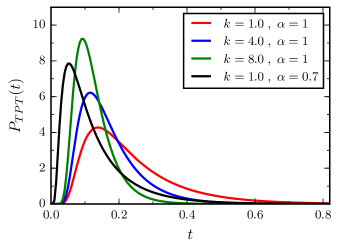
Fig.  3: Examples of TPT distributions $P_{TPT}(t)$ for $x_{0}=1$ and $\gamma=0.4$. Average TPT decreases with increasing energy barrier and decreasing $\alpha$. Typically, the distributions are obtained truncating the infinite series (22) to approx $n\leq 100$.

Fig.  4: Comparison between TPT distributions obtained with absorbing boundary conditions (Eq. (22) - solid lines) and free boundary conditions (Eq. (25) - dashed lines). The two expressions converge as $k$ increases, corresponding to an increase of the barrier height. The other parameters are $x_{0}=1$, $\gamma=0.4$ and $\alpha=1$.

4 The high barrier limit

The high barrier limit corresponds to the range of rescaled barrier heights $\Delta U\gg 1$. As mentioned in the Introduction for very high barriers one expects that TPT distributions are the same whether either free or absorbing boundary conditions are used. This is because stochastic trajectories will tend to cross the boundaries at $\pm x_{0}$ typically only once. The TPT distribution for a parabolic barrier with free boundaries was shown to be given by ²⁰

$$P_{TPT}(t)=-\dfrac{2}{\pi}\dfrac{\accentset{\mbox{.}}{G}(t)e^{-G^{2}(t)}}{1-Erf[\sqrt{\Delta U}]}\;,$$ (25)

where

$$G^{2}(t)\equiv\Delta U\dfrac{\theta(t)+1}{\theta(t)-1}\;.$$ (26)

and $\theta(t)$ the Mittag-Leffler function defined in (6). Figure 4 shows a comparison between Eq. (25) (dashed lines) and Eq. (22) (solid lines). The two expression tend indeed to the same limiting value as the barrier height increases (increasing $k$).

At long times, the Mittag-Leffler function converges to an exponential ⁴⁰ $\theta(t)\sim\exp(\Omega t)$ where we defined $\Omega\equiv(k/\eta_{\alpha})^{1/\alpha}$, which is an intrinsic rate set by the barrier stiffness $k$ and the noise amplitude $\eta_{\alpha}$. This implies that the free boundary distribution (25) decays asymptotically as ²⁰

$$P_{TPT}(t)\sim\exp(-\Omega t)$$ (27)

In the limit $t\to\infty$ the expression (22) is dominated by the lowest eigenvalue, hence it becomes

$$P_{TPT}(t)\sim\frac{\accentset{\mbox{.}}{\theta}(t)}{\left[\theta(t)\right]^{1-s_{0}}}\sim\exp(s_{0}\Omega t)$$ (28)

As discussed above, at high barrier $s_{n}$ converges to the quantum oscillator energy levels $s_{n}=-n-1$, which implies that (28) shows the same asymptotic decay as (27) in the high barrier limit. Note that the exponential decay (28) remains valid also for low barriers. In this case the decay rate is $|s_{0}|\Omega$, i.e. it differs from the intrinsic rate $\Omega$.

5 Fitting empirical distributions

TPT distributions obtained either from experiments or numerical simulations can be fitted to Eq. (22). An online tool performing the fits is freely available ⁴¹. In order to test the procedure we performed some Brownian Dynamics (BD) simulations for a particle moving in a double-well potential. We restricted the analysis to the Markovian case $\alpha=1$, which is easier to handle numerically as the noise is uncorrelated. Note, however, that the coordinate-dependent functions $Y_{n}(x)$ and the corresponding values of $s_{n}$ (whose calculations are computationally heavy) are independent of $\alpha$.

We considered the following piecewise parabolic potential (see Fig. 5b)

$$U(x)=\left\{\begin{array}[]{l}k(x+2x_{0})^{2}/2-kx_{0}^{2}/2\qquad x<-x_{0}\\ -kx^{2}/2+kx_{0}^{2}/2\qquad-x_{0}\leq x\leq x_{0}\\ k(x-2x_{0})^{2}/2-kx_{0}^{2}/2\qquad x>x_{0}\\ \end{array}\right.$$ (29)

which has two minima in $x=\pm 2x_{0}$ and a local maximum in $x=0$. $U(x)$ and its derivative are continuous, therefore there is no jump in the force which could be potentially harmful for the simulation.

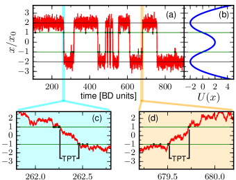
Fig.  5: a: Example of a BD trajectory of rescaled position $x/x_{0}$ vs. rescaled time $t/\beta\gamma x_{0}^{2}$ (this dimensionless variable is referred to as BD units in the graph axis). b: Plot of the piecewise parabolic potential (29) used in the simulation. c and d: Details of two parts of the trajectories emphasizing a transition path from $x_{0}$ to $-x_{0}$ (c) and from $-x_{0}$ to $x_{0}$ (d).

Figure 5a shows an example of a trajectory of rescaled position $x/x_{0}$ vs. rescaled time $t/\beta\gamma x_{0}^{2}$ (referred to as [BD units] in the graphs) obtained from BD simulations for a particle moving in the potential (29). The coordinate $x$ fluctuates between the two minima and the TPT are calculated from the crossings of the trajectories at $\pm x_{0}$ (see Fig. 5c and 5d). We tested Eq. (22) for several sets of the parameters $k$ and $\gamma$ (with $\alpha=1$). For each set we collected $10^{6}$ TPTs, from which a histogram was obtained. Figure 6 shows such a histogram (green bars ending with circles) for $\gamma=0.16$ and $\Delta U=1$. The solid red line is obtained by fitting the BD data to Eq. (22). The fit provides values of $\gamma$ and $\Delta U$ which are in close agreement to the input values (given in the caption of Fig. 6). The dashed line in Fig. 6 is a fit of the BD data to Eq. (25). Although the overall quality of the fit is good a closer look at the short time scales (inset (a)), the maximum (inset (b)) and the tail (inset (c)) show that Eq. (22) (solid lines) is a better fit to the data. Moreover the values of $\Delta U$ and $\gamma$ obtained from fitting the BD simulations to Eq. (25) deviate sensibly from the input data. For instance, one gets $\Delta U=1.57$ which is more than $50\%$ above the input value.

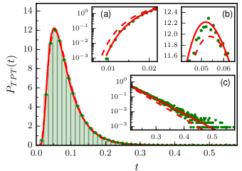
Fig.  6: Green bars: TPT histogram obtained from BD simulations with $\Delta U=1.0$ and $\gamma=0.16$. Red solid line: Best fit of the simulations to Eq. (22) yielding $\Delta U=1.0$ and $\gamma=0.16$ as fitting parameters. Red dashed line: Best fit of the simulations to Eq. (25) yielding $\Delta U=1.57$ and $\gamma=0.12$ as fitting parameters. Solid and dashed lines are hardly distinguishable on the scale of the main graph. The insets (a), (b) and (c) zoom in on the short time behavior, on the maximum and on the long time behavior of the TPT distribution showing that the solid line fits better the BD simulations (green circles) compared to the dashed line.

Table 1 summarizes the results of the fittings of the BD data. The first two columns give the values of $\Delta U$ and $\gamma$ used in the simulations. The two middle columns are the outputs of $\Delta U$ and $\gamma$ from fits of Eq. (22) and the the last two columns give the same parameters from fits of Eq. (25). An uncertainty on the fitted parameters is also given. The differences in the uncertainties in the two cases is due to a difference in the fitting procedure. While Eq. (25) has a simple analytical form and the search through the parameter space $(\Delta U,\gamma)$ for optimal fitting parameters is very fast and efficient, the fitting to Eq. (22) is much more complex. Each time a pair of values $(\Delta U,\gamma)$ is sampled one needs to compute the $s_{n}$ providing the absorbing boundary conditions $Y_{n}(\pm x_{0})=0$ and this has to be done for a sufficient number of terms so that one gets an accurate truncation of the infinite series. To avoid performing these calculations on the fly we considered a grid of fixed values $\Delta U_{k}=0.1k$ with $1\leq k\leq 200$ and $\gamma_{m}=0.01m$ with $1\leq m\leq 200$. We note that without any loss of generality one can set $x_{0}=1$ since

$$\int_{-x_{0}}^{+x_{0}}Y_{n}^{2}(x)dx=x_{0}\int_{-1}^{+1}\widetilde{Y_{n}}^{2}(y)dy\;,$$ (30)

where $\widetilde{Y_{n}}(y)\equiv Y_{n}(x_{0}\,y)$, and that the integral in the rhs term depends only on $\Delta U$. Hence from the $x_{0}=1$ case one can easily generalize the result to arbitrary $x_{0}$ with a simple rescaling.

Table 1:  Fitted values of $\Delta U$ and $\gamma$ on BD simulation data. The first two columns are the values used in the simulations. Columns $3$ and $4$ are obtained from fitting to Eq. (22) while columns $5$ and $6$ are from fitting to Eq. (25). Typically free boundary conditions (Eq. (25)) lead to an overestimate of the barrier height. This does not seem to be true for the case $\Delta U=4$, which is the highest value of the Table. However, it remains true if one fits to Eq. (25) while keeping $\gamma$ fixed to the input value.

BD simulations		Eq.(22) - Absorbing BC		Eq.(25) - Free BC
$\Delta U$	$\gamma$	$\Delta U\;(\pm 0.1)$	$\gamma\;(\pm 0.01)$	$\Delta U\;(\pm 0.01)$	$\gamma\;(\pm 0.01)$
$0.5$	$0.16$	$0.5$	$0.16$	$1.30$	$0.12$
$0.5$	$0.40$	$0.6$	$0.41$	$1.29$	$0.30$
$0.5$	$1.20$	$0.5$	$1.20$	$1.29$	$0.90$
$1.0$	$0.16$	$1.0$	$0.16$	$1.57$	$0.12$
$1.0$	$0.40$	$1.1$	$0.41$	$1.56$	$0.30$
$1.0$	$1.20$	$1.0$	$1.20$	$1.56$	$0.91$
$2.0$	$0.16$	$2.0$	$0.16$	$2.16$	$0.12$
$2.0$	$0.40$	$2.0$	$0.40$	$2.16$	$0.31$
$2.0$	$1.20$	$2.0$	$1.20$	$2.16$	$0.93$
$4.0$	$0.16$	$4.0$	$0.16$	$3.61$	$0.13$
$4.0$	$0.40$	$4.0$	$0.40$	$3.57$	$0.32$
$4.0$	$1.20$	$4.0$	$1.20$	$3.58$	$0.97$

For any sampled pair $(\Delta U_{k},\gamma_{m})$ the first $1000$ values of $s_{n}$ and of $\widetilde{Y_{n}}^{\prime}(\pm 1)$ were stored on a database. Using the stored data one can rapidly estimate the TPT distribution Eq. (22). Given an input distribution $\widetilde{P}(t)$ one obtains the optimal fitting values of $\Delta U$ and $\gamma$ by minimizing over the grid

$$\chi_{k,m}=\int_{0}^{\infty}dt\left[\widetilde{P}(t)-P_{TPT}^{AB}(t;\Delta U_{k},\gamma_{m})\right]^{2}P_{TPT}^{AB}(t;\Delta U_{k},\gamma_{m})\>,$$ (31)

where $P_{TPT}^{AB}(t;\Delta U_{k},\gamma_{m})$ is obtained from Eq. (22). Here one minimizes the squared difference of the two distributions and the multiplication by $P_{TPT}^{AB}(t;\Delta U_{k},\gamma_{m})$ ensure that more probable events have higher weight. The values of the third and fourth columns of Table 1 were obtained in this procedure, using for $\widetilde{P}(t)$ the distribution obtained by BD simulations. Obviously, as one uses a fixed grid of values for the parameters, the accuracy cannot exceed the grid spacing.

In dealing with complex systems, either experimental or numerical, only a limited sampling is feasible. In order to have some insights on the error of the parameters and their dependence on the sample size, we have binned the total $10^{6}$ TPTs obtained from BD simulations in subets of sizes $L=10^{3}$, $L=10^{4}$ and $L=10^{5}$. One obtains in this way $M=10^{6}/L$ independent samples of size $L$. To estimate the error we computed the standard deviations $\sigma_{\Delta U}$ and $\sigma_{\gamma}$ over the values of $\Delta U$ and $\gamma$ for the $M$ samples. The error was estimated as $\varepsilon_{\Delta U}\equiv\max(\sigma_{\Delta U},\Delta\Delta U)$ and $\varepsilon_{\gamma}\equiv\max(\sigma_{\gamma},\Delta\gamma)$, where $\Delta\Delta U=0.1$ and $\Delta\gamma=0.01$ are the grid spacings used. The data reported in Table 2 estimate the typical uncertainty expected for a given sampling size. For instance using a set of $L=10^{4}$ TPTs one expects an uncertainty of $0.1-0.2$ on $\Delta U$, while this error increases for smaller sets. For a reasonable accuracy on the fitting parameters from the TPT distribution one needs about $10^{4}$ values.

Finally, although this section discussed mainly the fitting of BD data, the same procedure can be used to fit distributions obtained from experiments. One just needs to use an experimentally determined distribution for $\widetilde{P}(t)$ in (31). An online server performing these fits is available ⁴¹.

Table 2:  Errors of the parameters evaluated for a given number of available TPTs, evaluated as discussed in the main text.

	$\varepsilon_{\Delta U}$				$\varepsilon_{\gamma}$
$(\Delta U,\gamma)$	$L=10^{5}$	$L=10^{4}$	$L=10^{3}$		$L=10^{5}$	$L=10^{4}$	$L=10^{3}$
$(0.5,0.16)$	0.1	0.14	0.30		0.01	0.01	0.015
$(0.5,0.40)$	0.1	0.12	0.32		0.01	0.01	0.027
$(0.5,1.20)$	0.1	0.1	0.31		0.01	0.025	0.082
$(1.0,0.16)$	0.1	0.14	0.44		0.01	0.01	0.025
$(1.0,0.40)$	0.1	0.13	0.37		0.01	0.01	0.029
$(1.0,1.20)$	0.1	0.11	0.36		0.01	0.027	0.085
$(2.0,0.16)$	0.1	0.15	0.45		0.01	0.01	0.012
$(2.0,0.40)$	0.1	0.17	0.46		0.01	0.011	0.031
$(2.0,1.20)$	0.1	0.13	0.44		0.01	0.026	0.083
$(4.0,0.16)$	0.1	0.2	0.6		0.01	0.01	0.02
$(4.0,0.40)$	0.1	0.2	0.63		0.01	0.013	0.03
$(4.0,1.20)$	0.1	0.2	0.64		0.01	0.029	0.083

6 Conclusions

In this paper we have derived an exact expression for the TPT distribution for a particle crossing a parabolic barrier in terms of the eigenfunctions and eigenvalues of the associated Fokker-Planck equation. We considered a power-law correlated noise characterized by an exponent $\alpha\leq 1$, see Eqs. (2) and (3), where the Markovian case is recovered in the limit $\alpha\to 1$. The TPT distribution is expressed as an infinite series (Eq. (22)) obtained by separating space and time coordinates, where the coordinate functions $Y_{n}(x)$ are independent of the value of $\alpha$. In contrast to previous work on TPT distributions we have explicitly taken into account absorbing boundary conditions, which implies $Y_{n}(\pm x_{0})=0$ at the end points of the transition paths $\pm x_{0}$. In a recent work ¹⁵ the TPT distribution was determined using a similar approach in which the eigenfunctions and eigenvalues of a Fokker Planck equation for a particle in a general potential landscape $V(x)$ were determined numerically. However in that work it was assumed that $D(t)\sim t^{\alpha-1}$ a result which is only correct in a linear potential or for an harmonic one at early times ⁴². For other potentials, the form of $D(t)$ is unknown and one can expect that the form chosen in ¹⁵ is valid in an early time regime where the diffusing particle sees a linear potential. In contrast, we have used the exact expression for $D(t)$ for a quadratic potential (Eq. (5)). Note that the coordinate-dependent eigenfunctions do not depend on $D(t)$.

In general, we expect that our result will be very well able to describe TPT-distributions that come from experiments or simulations on realistic models of proteins or nucleic acids if at least the transition path times are measured on intervals where the potential can be well approximated as a parabola. For this purpose a webtool performing analysis of TPT distributions has been made freely available ⁴¹. Deviations from the result obtained here could be caused by more complex free energy landscapes where, for example, the reaction coordinate has to cross more than one barrier or a multidimensional energy landscape.

References

- Berezhkovskii and Szabo 2005 A. Berezhkovskii and A. Szabo, J. Chem. Phys., 2005, 122, 014503.
- Dudko et al. 2006 O. K. Dudko, G. Hummer and A. Szabo, Phys. Rev. Lett., 2006, 96, 108101.
- Zhang et al. 2007 B. W. Zhang, D. Jasnow and D. M. Zuckerman, J. Chem. Phys., 2007, 126, 074504.
- Sega et al. 2007 M. Sega, P. Faccioli, F. Pederiva, G. Garberoglio and H. Orland, Phys. Rev. Lett., 2007, 99, 118102.
- Chung et al. 2009 H. S. Chung, J. M. Louis and W. A. Eaton, Proc. Natl. Acad. Sci. USA, 2009, 106, 11837–11844.
- Chaudhury and Makarov 2010 S. Chaudhury and D. E. Makarov, J. Chem. Phys., 2010, 133, 034118.
- Orland 2011 H. Orland, J. Chem. Phys., 2011, 134, 174114.
- Neupane et al. 2012 K. Neupane, D. B. Ritchie, H. Yu, D. A. N. Foster, F. Wang and M. T. Woodside, Phys. Rev. Lett., 2012, 109, 068102.
- Kim and Netz 2015 W. K. Kim and R. R. Netz, J. Chem. Phys., 2015, 143, 224108.
- Makarov 2015 D. E. Makarov, J. Chem. Phys., 2015, 143, 194103.
- Truex et al. 2015 K. Truex, H. S. Chung, J. M. Louis and W. A. Eaton, Phys. Rev. Lett., 2015, 115, 018101.
- Daldrop et al. 2016 J. O. Daldrop, W. K. Kim and R. R. Netz, EPL (Europhysics Letters), 2016, 113, 18004.
- Pollak 2016 E. Pollak, Phys. Chem. Chem. Phys., 2016, 18, 28872.
- Neupane et al. 2016 K. Neupane, D. A. Foster, D. R. Dee, H. Yu, F. Wang and M. T. Woodside, Science, 2016, 352, 239–242.
- Satija et al. 2017 R. Satija, A. Das and D. E. Makarov, J. Chem. Phys., 2017, 147, 152707.
- Berezhkovskii et al. 2017 A. M. Berezhkovskii, L. Dagdug and S. M. Bezrukov, J. Phys. Chem. B, 2017, 121, 5455.
- Laleman et al. 2017 M. Laleman, E. Carlon and H. Orland, J. Chem. Phys, 2017, 147, 214103.
- Neupane et al. 2017 K. Neupane, F. Wang and M. T. Woodside, Proc. Natl. Acad. Sci. USA, 2017, 201611602.
- Janakiraman 2018 D. Janakiraman, J. Phys. A: Math. Theor., 2018, 51, 285001.
- Carlon et al. 2018 E. Carlon, H. Orland, T. Sakaue and C. Vanderzande, arXiv:1806.11070, 2018.
- Neupane et al. 2018 K. Neupane, N. Q. Hoffer and M. T. Woodside, Phys. Rev. Lett., 2018, 121, 018102.
- Hummer 2004 G. Hummer, J. Chem. Phys., 2004, 120, 516–523.
- Dubbeldam et al. 2007 J. Dubbeldam, A. Milchev, V. Rostiashvili and T. A. Vilgis, EPL (Europhys. Lett.), 2007, 79, 18002.
- Sakaue 2007 T. Sakaue, Phys. Rev. E, 2007, 76, 021803.
- Panja et al. 2007 D. Panja, G. T. Barkema and R. C. Ball, Journal of Physics: Condensed Matter, 2007, 19, 432202.
- Dubbeldam et al. 2011 J. L. Dubbeldam, V. Rostiashvili, A. Milchev and T. A. Vilgis, Phys. Rev. E, 2011, 83, 011802.
- Walter et al. 2012 J.-C. Walter, A. Ferrantini, E. Carlon and C. Vanderzande, Phys. Rev. E, 2012, 85, 031120.
- Frederickx et al. 2014 R. Frederickx, T. In’t Veld and E. Carlon, Phys. Rev. Lett., 2014, 112, 198102.
- Vandebroek and Vanderzande 2015 H. Vandebroek and C. Vanderzande, Phys. Rev. E, 2015, 92, 060601.
- Sakaue et al. 2017 T. Sakaue, J.-C. Walter, E. Carlon and C. Vanderzande, Soft Matter, 2017, 13, 3174–3181.
- Goychuk and Hänggi 2007 I. Goychuk and P. Hänggi, Phys. Rev. Lett., 2007, 99, 200601.
- Wang and Tokuyama 2004 K. G. Wang and M. Tokuyama, Phys. A, 2004, 265, 341.
- Adelman 1976 S. A. Adelman, J. Chem. Phys., 1976, 64, 124.
- Hänggi and Thomas 1977 P. Hänggi and H. Thomas, Z. Phys. B, 1977, 26, 85.
- Hynes 1986 J. T. Hynes, J. Phys. Chem., 1986, 90, 3701.
- Abramowitz and Stegun 1964 M. Abramowitz and I. A. Stegun, Handbook of mathematical functions: with formulas, graphs, and mathematical tables, Courier Corporation, 1964, vol. 55.
- Brent 1973 R. P. Brent, Algorithms for Minimization Without Derivatives, Englewood Cliffs, NJ: Prentice-Hall, 1973.
-
38
For fixed and , the large -zeros of are given by
Setting , for even and , for odd leads to Eq. (24). - 39 NIST Digital Library of Mathematical Functions, http://dlmf.nist.gov/, Release 1.0.18 of 2018-03-27, F. W. J. Olver, A. B. Olde Daalhuis, D. W. Lozier, B. I. Schneider, R. F. Boisvert, C. W. Clark, B. R. Miller and B. V. Saunders, eds.
- Haubold et al. 2011 H. J. Haubold, A. M. Mathai and R. K. Saxena, Journal of Applied Mathematics, 2011, 2011, 298628.
- 41 See http://itf.fys.kuleuven.be/~tptwithab/.
- 42 Expanding Eq. (5) for short times and using the properties of the Mittag-Leffler function one gets indeed .