1

Decreasing the size of the Restricted Boltzmann machine

Yohei Saito
yoheis@sat.t.u-tokyo.ac.jp
Institute of Industrial Science, The University of Tokyo, 4-6-1, Komaba,
Meguro-ku, Tokyo 153-8505 Japan
Takuya Kato
takuya.kato.origami@gmail.com
Graduate School of Information Science and Technology,
Department of Mathematical informatics, The University of Tokyo, 7-3-1, Hongo,
Bunkyo-ku, Tokyo 113-8654, Japan

Abstract

In this paper, we propose a method to decrease the number of hidden units of the restricted Boltzmann machine while avoiding a decrease in the performance quantified by the Kullback-Leibler divergence. Our algorithm is then demonstrated by numerical simulations.

1 Introduction

The improvement of computer performance enables utilization of the exceedingly high representational powers of neural networks. Deep neural networks have been applied to various types of data, e.g. images, speech, and natural language, and have achieved great success (Bengio . (2013); He . (2016); Vaswani . (2017); Goodfellow . (2014); Oord . (2016)) both in discrimination and generation tasks. To increase performance, which stems from the hierarchical structures of neural networks (Hestness . (2017)), network size becomes larger, and computational burdens increase. Thus, demands for decreasing the network size are growing. In particular, various methods were proposed for compressing the sizes of discriminative models (Han . (2015); Guo . (2016); Cheng . (2017)). However, compression of generative models (Berglund . (2015)) has scarcely been discussed.

Discriminative models provide the probabilities that into which class the given data are classified (Christopher (2016)), and in most cases, their learning requires a supervisor, namely, a dataset with classification labels attached by humans. Thus, outputs of discriminative models can be intuitively interpreted by humans. However, some data are difficult for humans to properly classify. Even if possible, hand-labeling tasks are a troublesome labor. In such cases, generative models with unsupervised learning are effective, since they automatically find the data structure without hand-labels by learning the joint probabilities of data and classes. Therefore, it is expected that the compression of generative models with unsupervised learning will be required in the future. Furthermore, if the system’s performance can be preserved during compression, then the network size can be decreased while it is in use. To approximately maintain performance throughout compression, we consider removing the part of the system after decreasing its contribution to the overall performance. Our approach differs from the procedures in previous studies (Han . (2015); Guo . (2016); Cheng . (2017); Berglund . (2015)) that retrain systems after removing a part that contributes little to their performance.

In this paper, we deal with the restricted Boltzmann machine (RBM) (Smolensky (1986); Fischer  Igel (2012)). The RBM is one of the most important generative models with unsupervised learning, from the viewpoints of not only machine learning history (Bengio . (2013)) but also its wide applications, e.g., generation of new samples, classification of data (Larochelle  Bengio (2008)), feature extraction (Hinton  Salakhutdinov (2006)), pretraining of deep neural networks (Hinton  Salakhutdinov (2006); Hinton . (2006); Salakhutdinov  Larochelle (2010)), and solving many-body problems in physics (Carleo  Troyer (2017); Tubiana  Monasson (2017)). The RBM consists of visible units that represent observables, e.g., pixels of images, and hidden units that express correlations between visible units. An objective of the RBM is to generate plausible data by imitating the probability distribution from which true data are sampled. In this case, the performance of the RBM is quantified by the difference between the probability distribution of data and that of visible variables of the RBM, and it can be expressed by the Kullback-Leibler divergence (KLD). The RBM can exactly reproduce any probability distribution of binary data if it has a sufficient number of hidden units (Le Roux  Bengio (2008)). However, a smaller number of hidden units may be enough to capture the structure of the data. Therefore, in this paper, we aim to practically decrease the number of hidden units while avoiding an increase in the KLD between the model and data distributions (Figure 1).

The outline of this paper is as follows. In section 2, we give a brief review of the RBM. In section 3, we evaluate the deviation of the KLD associated with node removal and propose a method that decreases the number of hidden units while avoiding an increase in the KLD. Numerical simulations are demonstrated in section 4, and we summarize this paper in section 5. The details of calculations are shown in Appendices.

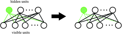
Figure 1: The graphical model of the RBM is shown. While approximately preserving the KLD, the target hidden unit and its edges (green) are removed from the main body of the RBM (from the left to right panel).

2 Brief introduction of the RBM

In this section, we briefly review the RBM, which is a Markov random field that consists of visible units, ${}^{t}\!{\boldsymbol{v}}=(v_{1},\ldots,v_{M})\in\{0,1\}^{M}\,$, and hidden units, ${}^{t}\!{\boldsymbol{h}}=(h_{1},\ldots,h_{N})\in\{0,1\}^{N}\,$. The joint probability that a configuration $({\boldsymbol{v}},{\boldsymbol{h}})$ is realized, $p({\boldsymbol{v}},{\boldsymbol{h}})\,$, is given by the energy function, $E({\boldsymbol{v}},{\boldsymbol{h}})\,$, as follows:

$$E({\boldsymbol{v}},{\boldsymbol{h}}) = -{}^{t}\!{\boldsymbol{b}}\,{\boldsymbol{v}}-{}^{t}\!{\boldsymbol{c}}\,{\boldsymbol{h}}-{}^{t}\!{\boldsymbol{v}}\,W\,{\boldsymbol{h}}$$ (1)

$$= -\sum_{i=1}^{M}b_{i}\,v_{i}-\sum_{j=1}^{N}c_{j}\,h_{j}-\sum_{i=1}^{M}\sum_{j=1}^{N}v_{i}\,w_{ij}\,h_{j}\,,$$

$$p({\boldsymbol{v}},{\boldsymbol{h}}) = \frac{{\rm e}^{-E({\boldsymbol{v}},{\boldsymbol{h}})}}{\sum_{{\boldsymbol{v}}^{\prime},{\boldsymbol{h}}^{\prime}}{\rm e}^{-E({\boldsymbol{v}}^{\prime},{\boldsymbol{h}}^{\prime})}}\,,$$ (2)

where ${}^{t}\!{\boldsymbol{b}}=(b_{1},\ldots,b_{M})\in\mathbb{R}^{M}$ and ${}^{t}\!{\boldsymbol{c}}=(c_{1},\ldots,c_{N})\in\mathbb{R}^{N}$ are the biases of the visible and hidden units, respectively, and $W=(w_{ij})\in\mathbb{R}^{M\times N}$ is the weight matrix . Below, we abbreviate all of the RBM parameters, ${\boldsymbol{b}}\,$, ${\boldsymbol{c}}\,$, and $W\,$, as ${\boldsymbol{\xi}}\,$.

By properly tuning ${\boldsymbol{\xi}}\,$, the probability distribution of the visible variables, $p({\boldsymbol{v}})=\sum_{\boldsymbol{h}}p({\boldsymbol{v}},{\boldsymbol{h}})\,$, can approximate the unknown probability distribution that generates real data, $q({\boldsymbol{v}})\,$. The performance of the RBM can be measured by the KLD of $p({\boldsymbol{v}})$ from $q({\boldsymbol{v}})\,$,

$$D_{\rm KL}({q}||{p})=\sum_{\boldsymbol{v}}q({\boldsymbol{v}})\,\ln\frac{q({\boldsymbol{v}})}{p({\boldsymbol{v}})}\,.$$ (3)

Hence, learning of the RBM is performed by updating the RBM parameters ${\boldsymbol{\xi}}$ so as to decrease the KLD. The gradient descent method is often employed to decrease the KLD as

$${\boldsymbol{\xi}}^{s+1}={\boldsymbol{\xi}}^{s}-\lambda\,\nabla_{\boldsymbol{\xi}}D_{\rm KL}({q}||{p})|_{{\boldsymbol{\xi}}={\boldsymbol{\xi}}^{s}}\,,$$ (4)

where ${\boldsymbol{\xi}}^{s}$ and ${\boldsymbol{\xi}}^{s+1}$ denote the RBM parameters at the $s$-th and $(s+1)$-th step of the learning process, respectively. A learning rate is represented by $\lambda\,(>0)\,$, and $\nabla_{\boldsymbol{\xi}}D_{\rm KL}({q}||{p})|_{{\boldsymbol{\xi}}={\boldsymbol{\xi}}^{s}}$ denotes the gradient of the KLD with respect to ${\boldsymbol{\xi}}$ at the $s$-th step. The gradient with respect to $b_{i},c_{j},$ and $w_{ij}$ can be written as

$$\frac{\partial D}{\partial b_{i}} = -\sum_{\boldsymbol{v}}v_{i}\,q({\boldsymbol{v}})+\left<v_{i}\right>_{p}\,,$$ (5)

$$\frac{\partial D}{\partial c_{j}} = -\sum_{\boldsymbol{v}}q({\boldsymbol{v}})\,p(h_{j}=1|{\boldsymbol{v}})+\left<h_{j}\right>_{p}\,,$$ (6)

$$\frac{\partial D}{\partial w_{ij}} = -\sum_{\boldsymbol{v}}v_{i}\,q({\boldsymbol{v}})\,p(h_{j}=1|{\boldsymbol{v}})+\left<v_{i}h_{j}\right>_{p}\,,$$ (7)

where $D_{\rm KL}({q}||{p})$ is abbreviated as $D$ and the expectation value with respect to $p({\boldsymbol{v}},{\boldsymbol{h}})$ as $\left<\cdot\right>_{p}\,$. The conditional probability, $p(h_{j}|{\boldsymbol{v}})\,$, is given by

$$p(h_{j}|{\boldsymbol{v}})=\frac{{\rm e}^{(c_{j}+\sum_{i}v_{i}w_{ij})\,h_{j}}}{1+{\rm e}^{c_{j}+\sum_{i}v_{i}w_{ij}}}\,.$$ (8)

If $D$ and $\nabla_{\boldsymbol{\xi}}D$ can be obtained, then the RBM reaches some local minimum of the KLD through a parameter update. However, neither of them can be calculated, since they not only contain the unknown probability $q({\boldsymbol{v}})$ but also the sum with respect to the large state space of the RBM. Thus, in Eq. (5), Eq. (6), and Eq. (7), One approximates $q({\boldsymbol{v}})$ by empirical distribution, or more practically, mini-batch, which are samples from the empirical distribution. One also evaluates the expectation values with respect to $p({\boldsymbol{v}},{\boldsymbol{h}})$, which are computationally expensive, by using the realizations obtained from Gibbs sampling, e.g. contrastive divergence (CD) (Hinton (2002)), persistent CD (PCD) (Tieleman (2008)), fast PCD (Tieleman  Hinton (2009)), and block Gibbs sampling with tempered transition (Salakhutdinov (2009)) or with parallel tempering (Cho . (2010); Desjardins . (2010)). Block Gibbs sampling in the RBM effectively updates the configuration, $({\boldsymbol{v}},{\boldsymbol{h}})\,$, by repeatedly using the conditional probabilities,

$$p({\boldsymbol{h}}|{\boldsymbol{v}}) = \prod_{j}p(h_{j}|{\boldsymbol{v}})=\prod_{j}\frac{{\rm e}^{(c_{j}+\sum_{i}v_{i}w_{ij})\,h_{j}}}{1+{\rm e}^{c_{j}+\sum_{i}v_{i}w_{ij}}}\,,$$ (9)

$$p({\boldsymbol{v}}|{\boldsymbol{h}}) = \prod_{i}p(v_{i}|{\boldsymbol{h}})=\prod_{i}\frac{{\rm e}^{(b_{i}+\sum_{j}h_{j}w_{ij})\,v_{i}}}{1+{\rm e}^{b_{i}+\sum_{j}h_{j}w_{ij}}}\,,$$ (10)

as transition matrices. In many cases, CD and PCD employ only a few block Gibbs sampling steps. In addition to $\nabla_{\boldsymbol{\xi}}D\,$, the KLD, which represents the performance of the RBM, is also intractable. Therefore, in order to monitor the learning progress, a different quantity is employed which can be considered to correlate to the KLD to a certain degree, e.g. the reconstruction error (Bengio . (2007); Taylor . (2007); Hinton (2012)), the product of the two probabilities ratio (Buchaca . (2013)), and the likelihood of a validation set obtained by tracking the partition function (Desjardins . (2011)).

3 Removal of hidden units

3.1 Removal cost and its gradient

The goal of this paper is not to propose a new method for optimization of the KLD, but to decrease the number of hidden units while avoiding an increase in the KLD. Suppose an RBM achieves, if not optimal, sufficient performance after the learning process at a fixed number of hidden units, $N\,$. Next, we remove the $k$-th hidden unit of the RBM so as not to increase the KLD. In order to compare the performances of two RBMs whose $k$-th hidden unit does or does not exist, we introduce ${\boldsymbol{h}}_{\backslash k}$ as a configuration of hidden units except for $h_{k}\,$, ${}^{t}\!{\boldsymbol{h}}_{\backslash k}=(h_{1},\ldots,h_{k-1},h_{k+1},\ldots,h_{N})\,$. The energy function and the probability distribution of the RBM after removal are given by

$$E_{\backslash k}({\boldsymbol{v}},{\boldsymbol{h}}_{\backslash k}) = -\sum_{i}b_{i}\,v_{i}-\sum_{j\neq k}c_{j}\,h_{j}-\sum_{i}\sum_{j\neq k}v_{i}\,w_{ij}\,h_{j}$$ (11)

$$= E({\boldsymbol{v}},{\boldsymbol{h}})|_{h_{k}=0}\,,$$

$$p_{\backslash k}({\boldsymbol{v}},{\boldsymbol{h}}_{\backslash k}) = \frac{{\rm e}^{-E_{\backslash k}({\boldsymbol{v}},{\boldsymbol{h}}_{\backslash k})}}{\sum_{{\boldsymbol{v}}^{\prime},{\boldsymbol{h}}^{\prime}_{\backslash k}}{\rm e}^{-E_{\backslash k}({\boldsymbol{v}}^{\prime},{\boldsymbol{h}}^{\prime}_{\backslash k})}}\,.$$ (12)

Then, we define a removal cost, $C_{k}\,$, as the difference of the KLD before and after removing the $k$-th hidden unit:

$$C_{k} \equiv D_{\rm KL}({q}||{p_{\backslash k}})-D_{\rm KL}({q}||{p})$$ (13)

$$= \sum_{\boldsymbol{v}}q({\boldsymbol{v}})\,\ln\frac{q({\boldsymbol{v}})}{p_{\backslash k}({\boldsymbol{v}})}-\sum_{\boldsymbol{v}}q({\boldsymbol{v}})\,\ln\frac{q({\boldsymbol{v}})}{p({\boldsymbol{v}})}$$

$$= -\sum_{\boldsymbol{v}}q({\boldsymbol{v}})\,\ln p(h_{k}=0|{\boldsymbol{v}})+\ln p(h_{k}=0)\,.$$

The details of the calculation and removal cost for several hidden units are shown in Appendix A. Thus, if $C_{k}$ satisfies $C_{k}\leq 0\,$, then the $k$-th hidden unit can be removed without increasing the KLD.

In most cases, however, there are no hidden units with non-positive removal costs. Thus, before removing a hidden unit, we first decrease its removal cost without increasing the KLD . For this purpose, we naively determine the parameter update at the $s$-th step in a removal process, $\Delta{\boldsymbol{\xi}}^{s}\,$, so that both $C_{k}$ and the KLD decrease at ${\cal O}(|\Delta{\boldsymbol{\xi}}^{s}|)$ (see Appendix B):

$$\Delta\xi_{i}^{s} = -\nu\cdot\theta\left(\frac{\partial D}{\partial\xi_{i}}\,\frac{\partial C_{k}}{\partial\xi_{i}}\right)\cdot\frac{\partial D}{\partial\xi_{i}}\,\bigg{|}_{{\boldsymbol{\xi}}={\boldsymbol{\xi}}^{s}}\,,$$ (14)

$$\theta(x) = \begin{cases}1&(x\geq 0)\\ 0&(x<0)\end{cases}\,,$$ (15)

where $\nu\,(>0)$ is the parameter change rate, and $\theta(x)$ is the step function. Evaluation of $\nabla_{\boldsymbol{\xi}}D$ can be performed using Eq. (5), Eq. (6), and Eq. (7), and $\nabla_{\boldsymbol{\xi}}C_{k}$ can be written as

$$\frac{\partial C_{k}}{\partial b_{i}} = \left<v_{i}\right>_{\bar{p}}-\left<v_{i}\right>_{p}\,,$$ (16)

$$\frac{\partial C_{k}}{\partial c_{j}} = \sum_{\boldsymbol{v}}q({\boldsymbol{v}})\,p(h_{k}=1|{\boldsymbol{v}})\,\delta_{kj}+\left<h_{j}\right>_{\bar{p}}-\left<h_{j}\right>_{p}\,,$$ (17)

$$\frac{\partial C_{k}}{\partial w_{ij}} = \sum_{\boldsymbol{v}}q({\boldsymbol{v}})\,v_{i}\,p(h_{k}=1|{\boldsymbol{v}})\,\delta_{kj}+\left<v_{i}h_{j}\right>_{\bar{p}}-\left<v_{i}h_{j}\right>_{p}\,,$$ (18)

where $\delta_{kj}$ is the Kronecker delta, and $\left<\cdot\right>_{p}$ and $\left<\cdot\right>_{\bar{p}}$ denote expectation values with respect to $p({\boldsymbol{v}},{\boldsymbol{h}})$ and $\bar{p}\equiv p({\boldsymbol{v}},{\boldsymbol{h}}_{\backslash k}|h_{k}=0)\,$, respectively. If $C_{k}\leq 0$ is satisfied after parameter updates, then the $k$-th hidden unit can be removed without increasing the KLD. When all of the RBM parameters satisfy $\partial D/\partial\xi_{i}\cdot\partial C_{k}/\partial\xi_{i}<0\,$, then $C_{k}$ cannot decrease without increasing the KLD, and the parameter update is stopped ($\Delta{\boldsymbol{\xi}}={\boldsymbol{0}}$) .

Note two properties of $C_{k}\,$. First, $-C_{k}$ can be interpreted as an additional cost of a new node. Thus, it may be employed when new nodes are added into an RBM whose performance is insufficient. Secondly, Eq. (13) can be applied to the Boltzmann machine (BM) (Ackley . (1987)), which is expressed as a complete graph consisting of visible and hidden units, and a special case of the BM called the deep Boltzmann machine (DBM) (Salakhutdinov  Hinton (2009)), which has hierarchical hidden layers with neighboring interlayer connections. However, in these cases, calculation of the conditional probability, $p(h_{k}=0|{\boldsymbol{v}})\,$, and gradients with respect to the model parameters are computationally expensive compared to the RBM.

3.2 Practical removal procedure

The removal process proposed in the previous subsection preserves the performance when $C_{k}\,$, $\nabla_{\boldsymbol{\xi}}C_{k}\,$, and $\nabla_{\boldsymbol{\xi}}D$ can be accurately evaluated. However, in most cases, $C_{k}$ and $\nabla_{\boldsymbol{\xi}}C_{k}$ are approximated using Gibbs sampling, as with $\nabla_{\boldsymbol{\xi}}D\,$. Thus, in order to reflect the variances of Gibbs sampling, we change both the parameter update rule and removal condition, Eq. (14) and Eq. (13), into more effective forms.

First, we modify the parameter update rule, Eq. (14), which may increase $D$ due to two reasons. The first is the inaccuracy of Gibbs sampling, and the second is the contribution from higher-order derivative terms of ${\cal O}(|\Delta{\boldsymbol{\xi}}|^{2})\,$. These problems also arise in the learning process. However, even if $D$ increases, it can decrease again through the update rule, Eq. (4). Since the difference between Eq. (4) and Eq. (14) is solely the existence of the step function, similar behavior is expected in the removal process. Unfortunately, Eq. (14) frequently increases $D$ due to the following. Since the removal cost is defined as the change in the KLD through node removal, it can be interpreted as the contribution of the node to the performance. Hence, when the performance increases, removal costs are expected to increase. This means that in the RBM parameter space, there are few directions along which both $D$ and $C_{k}$ decrease. However, since the step function in Eq. (14) allows the parameter update solely along these few directions, there are few opportunities to decrease $D\,$. Therefore, once $D$ increases, it rarely decreases by Eq. (14). As a result, a successive increase of $D$ occurs. In order to maintain the performance, we probabilistically accept updates which increase $C_{k}\,$. That is, we change the step function in Eq. (14), which gives either $0$ or $1$ deterministically, into a random variable, $z_{i}\in\{0,\,1\}\,$. Next, we determine the probability that $z_{i}$ takes $1\,$, that is, the acceptance probability of updates. The modified update rule is required to return to Eq. (14) when Gibbs sampling estimates are exactly obtained. For this purpose, we employ the ratio of the mean to the standard deviation and determine the modified update rule by

$$\overline{\Delta\xi_{i}^{s}} = -\nu\,z_{i}\,\overline{\partial_{i}D}\,|_{{\boldsymbol{\xi}}={\boldsymbol{\xi}}^{s}}\,,$$ (19)

$$p(z_{i}=1) = {\rm sig}\left(\frac{\sqrt{S}\cdot\overline{\partial_{i}D}}{\overline{\sigma_{D,i}}}\cdot\frac{\sqrt{S}\cdot\overline{\partial_{i}C_{k}}}{\overline{\sigma_{C,i}}}\right)\,,$$ (20)

$${\rm sig}(x) = \frac{{\rm e}^{x}}{1+{\rm e}^{x}}\,,$$ (21)

where $S$ is the number of Gibbs samples, and $\overline{\partial_{i}D}$ and $\overline{\partial_{i}C_{k}}$ represent sample means of $\partial D/\partial\xi_{i}$ and $\partial C_{k}/\partial\xi_{i}$, respectively. The unbiased standard deviations of $\partial D/\partial\xi_{i}$ and $\partial C_{k}/\partial\xi_{i}$ are denoted by $\overline{\sigma_{D,i}}$ and $\overline{\sigma_{C,i}}\,$, respectively. As the number of samples increases, Eq. (19) returns to Eq. (14) .

Secondly, we modify the removal condition, Eq. (13). Since node removal irreversibly decreases the representational power of the RBM, we carefully verify whether $C_{k}\leq 0$ is satisfied. However, since the logarithmic function in the second term of Eq. (13) drastically decreases in $p(h_{k}=0)<1\,$, a small sampling error in $p(h_{k}=0)$ results in a large error in $\ln p(h_{k}=0)\,$, which makes it difficult to evaluate the removal cost accurately by Gibbs sampling. Therefore, we employ an upper bound of $C_{k}$ as an effective removal cost, $C_{k}^{\prime}\,$:

$$C_{k} = -\sum_{\boldsymbol{v}}q({\boldsymbol{v}})\,\ln p(h_{k}=0|{\boldsymbol{v}})+\ln[1-p(h_{k}=1)]$$ (22)

$$\leq -\sum_{\boldsymbol{v}}q({\boldsymbol{v}})\,\ln p(h_{k}=0|{\boldsymbol{v}})-p(h_{k}=1)$$

$$\equiv C^{\prime}_{k}\,.$$

Then, consider the approximation of $C^{\prime}_{k}$ by Gibbs sampling,

$$\overline{C^{\prime}_{k}} \equiv -\frac{1}{S}\,\sum_{\alpha=1}^{S}\ln p(h_{k}=0|{\boldsymbol{v}}^{\alpha})-\frac{1}{S}\,\sum_{\alpha=1}^{S}h_{k}^{\alpha}\,,$$ (23)

where $\alpha$ is the sample index. Since samplings from $q({\boldsymbol{v}})$ and $p({\boldsymbol{v}},{\boldsymbol{h}})$ are independent, the first and second terms of Eq. (23) have no correlations. Thus, when the sampling size, $S\,$, is sufficiently large, the probability distribution of $\overline{C^{\prime}_{k}}$ can be approximated by the normal distribution, due to the central limit theorem:

$$\overline{C^{\prime}_{k}} \sim {\cal N}\left(C^{\prime}_{k},\frac{\sigma_{1}^{2}}{S}+\frac{\sigma_{2}^{2}}{S}\right)\,,$$ (24)

$$\sigma_{1}^{2} = \sum_{\boldsymbol{v}}q({\boldsymbol{v}})\,\left[\ln p(h_{k}=1|{\boldsymbol{v}})\right]^{2}-\left[\sum_{\boldsymbol{v}}q({\boldsymbol{v}})\,\ln p(h_{k}=1|{\boldsymbol{v}})\right]^{2}\,,$$ (25)

$$\sigma_{2}^{2} = p(h_{k}=1)-[p(h_{k}=1)]^{2}\,,$$ (26)

where ${\cal N}(\mu,\sigma^{2})$ denotes the normal distribution. The unbiased standard deviation of $\overline{C^{\prime}_{k}}$ is given by

$$\overline{\sigma_{C^{\prime}_{k}}}=\sqrt{\frac{\overline{\sigma_{1}^{2}}+\overline{\sigma_{2}^{2}}}{S}}\,,$$ (27)

where $\overline{\sigma_{1}^{2}}$ and $\overline{\sigma_{2}^{2}}$ are the unbiased variances of $\ln p(h_{k}|{\boldsymbol{v}})$ and $h_{k}\,$, respectively. Using $\overline{C^{\prime}_{k}}$ and $\overline{\sigma_{C^{\prime}_{k}}}$, we change the removal criterion from $C_{k}\leq 0$ into $\overline{C^{\prime}_{k}}+a\,\overline{\sigma_{C^{\prime}_{k}}}\leq 0\,$, where $a$ tunes the confidence intervals of $C^{\prime}_{k}\,$. By increasing $a\,$, we can decrease the probability that a hidden unit is wrongly removed when its true removal cost is positive, $C_{k}>0\,$. When $\overline{\sigma_{C^{\prime}_{k}}}/D$ is not small, this incorrect removal may harm the performance. Thus, a large $a$ is used to decrease the probability of an incorrect removal.

In summary, our node removal procedure is as follows (Alg. 1). First, we remove all hidden units that satisfy the modified removal condition. Then, at each parameter update step, we choose the smallest removal cost and decrease it using Eq. (19) until a hidden unit can be removed. The source code is available on GitHub at https://github.com/snsiorssb/RBM.

Algorithm 1 Node removal procedure

1:for number of removing iterations do

2:     repeat

3:         obtain $S$ realizations, $({\boldsymbol{v}}^{1},{\boldsymbol{h}}^{1}),\ldots,({\boldsymbol{v}}^{S},{\boldsymbol{h}}^{S})\,$ by $n$-step block Gibbs sampling (PCD-$n$).

4:         evaluate $\overline{C^{\prime}_{j}}$ for all remaining hidden units by using Eq. (23).

5:         determine a node to be removed, $k=\mathop{\rm arg~{}min}\limits_{j}\overline{C^{\prime}_{j}}\,$.

6:         evaluate $\overline{\sigma_{C^{\prime}_{k}}}$ by using Eq. (27).

7:         if $\overline{C^{\prime}_{k}}+a\,\overline{\sigma_{C^{\prime}_{k}}}\leq 0$ then

8:              remove the target node

9:              obtain $S$ realizations by Gibbs sampling (tempered transition, from $\beta_{0}=1$ to $\beta_{1}$ divided by $l$ intervals).

10:         end if

11:     until $\overline{C^{\prime}_{j}}+a\,\overline{\sigma_{C^{\prime}_{j}}}>0$ for any $j\,$.

12:     evaluate $\overline{\partial_{i}D}\,$, $\overline{\partial_{i}C_{k}}\,$, $\overline{\sigma_{D,i}}\,$, and $\overline{\sigma_{C,i}}\,$.

13:     determine $\overline{\Delta{\boldsymbol{\xi}}}$ from Eq. (19).

14:     ${\boldsymbol{\xi}}^{s+1}={\boldsymbol{\xi}}^{s}-\nu\,\overline{\Delta{\boldsymbol{\xi}}}\,$.

15:end for

4 Numerical simulation

In this section, we show that the proposed algorithm does not spoil the performance of the RBMs by using two different datasets. First, we used the $3\times 3$ Bars-and-Stripes dataset (MacKay  Mac Kay (2003)) (Fig. 2), which is small enough to allow calculation of the exact KLD during the removal processes. Next, we employed MNIST dataset of handwritten images (LeCun  Cortes (1998)) and verified that our algorithm also works in realistic-size RBMs.

Since parameter update after sufficient learning slightly changes $p({\boldsymbol{v}},{\boldsymbol{h}})\,$, it can be considered that short Markov chains are enough for convergence to $p({\boldsymbol{v}},{\boldsymbol{h}})$ after parameter updates. Thus, we used PCD (Tieleman (2008)) with $n$-step block Gibbs sampling (PCD-$n$) in both learning and removal processes, except for samplings immediately after a node removal. However, a change of $p({\boldsymbol{v}},{\boldsymbol{h}})$ caused by node removal is expected to be larger than that caused by parameter updates. Hence, PCD-$n$ with small $n$ may not converge to $p({\boldsymbol{v}},{\boldsymbol{h}})$ and may fail to sample from $p({\boldsymbol{v}},{\boldsymbol{h}})$ immediately after node removals. Thus, we carefully performed Gibbs sampling using tempered transition (Salakhutdinov (2009); Neal (1996)) at these times. In tempered transition, we linearly divided the inverse temperature from $\beta_{0}=1$ to $\beta_{1}=0.9$ into $l=100$ intervals. We did not use a validation set for early stopping or hyperparameter searches in both the learning and removal processes.

Figure 2: Examples of $3\times 3$ Bars-and-Stripes images are shown, which are generated as follows. First, a white square of $A\times A$ pixel is prepared. Next, each column of the square is painted black with probability $1/2\,$. Finally, the square is rotated $90^{\circ}$ with probability $1/2\,$. For $A=3\,$, $14$ different images are created.

4.1 Bars-and-Stripes

An artificial dataset called Bars-and-Stripes was used to demonstrate that our algorithm effectively works when the data distribution is completely known. Thus, we did not divide the dataset into training and test sets. First, we trained the RBM with $M=9$ visible units and $N=30$ hidden units using PCD-5 and PCD-1 with a batch size of $100$ and a fixed learning rate, $\lambda=10^{-2}\,$. After $50,000$ learning steps, we performed removal processes starting from the same trained RBM with a batch size of $1,000$ and a fixed parameter change rate, $\nu=10^{-2}\,$. During the beginning of the removal process, the typical value of $\overline{\sigma_{C^{\prime}_{k}}}/D$ was not small, that is, $\overline{\sigma_{C^{\prime}_{k}}}/D\sim 0.1\,$. Thus, we employed a strict removal criterion, $\overline{C_{k}^{\prime}}+3\,\overline{\sigma_{C^{\prime}_{k}}}\leq 0\,$.

The results are shown in Figures 3, 4, and 5. We stopped the removal processes after $10,000,000$ steps in Figure 3 and after $5,000,000$ steps in Figures 4 and 5. The removal procedure employing PCD-5 slowly decreases $N$ with small fluctuations of the KLD in all five trials (Figure 3). In particular, the removal cost in Figure 3 shows that if a hidden unit with the smallest removal cost is removed before it decreases, then the KLD increases approximately sevenfold. This result clearly shows that the update rule, Eq. (19), is useful for maintaining the performance during the removal processes. The removal procedure employing PCD-1 decreases $N$ more rapidly while approximately preserving the KLD in six out of eight trials (Figure 4), although some sharp peaks appear in the change of the KLD after node removals. However, two out of eight trials that employed PCD-1 fail to preserve the KLD (Figure 5).

First, we discuss the sharp peaks observed in Figure 4, which resulted from inaccurate estimates of $C^{\prime}_{k}$ or $\overline{\Delta{\boldsymbol{\xi}}}\,$. In order to distinguish among them, we enlarge peaks in the change of the KLD (Figure 6) and find that these peaks were caused by the failure of Gibbs sampling in parameter updates immediately after node removals rather than node removals themselves. This behavior supports the assumption that the change of $p({\boldsymbol{v}},{\boldsymbol{h}})$ caused by node removal can be large and can result in failure of Gibbs sampling. Nevertheless, owing to the tempered transition, most of the parameter updates after node removal produced rather small peaks in Figure 4.

Next, we discuss large fluctuations of the KLD in Figure 5. Failure of Gibbs sampling through parameter updates is expected to occur more frequently as the removal process continues for the same reason as in the learning process (Fischer  Igel (2010); Desjardins . (2010)). It can be considered that the problem in the learning process arises as follows. At the beginning of the learning process, the RBM parameters are approximately zero, and $p({\boldsymbol{v}})$ is almost a uniform distribution. As the leaning proceeds, each component of ${\boldsymbol{\xi}}$ is expected to move away from zero in order to adjust $p({\boldsymbol{v}})$ to the data distribution, $q({\boldsymbol{v}})\,$. In the removal process, components of ${\boldsymbol{\xi}}$ are also expected to move away from zero in order that the remaining system compensates for the roles of the removed hidden units. As one can find from Eq. (9) and Eq. (10), the transition matrices used in MCMC, $p({\boldsymbol{h}}|{\boldsymbol{v}})$ and $p({\boldsymbol{v}}|{\boldsymbol{h}})\,$, take almost either $0$ or $1$ in the region where $|{\boldsymbol{\xi}}|$ is large. Therefore, block Gibbs sampling behaves almost deterministically. Hence, dependence on the initial condition remains for a long time, or equivalently, it takes a long time to converge to $p({\boldsymbol{v}},{\boldsymbol{h}})$ even after a one-step parameter update in the large $|{\boldsymbol{\xi}}|$ region. Thus, the model distribution after parameter update, from which we should sample, may be quite different from the probability distribution after a few block Gibbs sampling steps. As a result, parameters are updated using inaccurate Gibbs samples. If these deviations are corrected by subsequent parameter updates, then the KLD decreases again. However, if the failure of Gibbs sampling continues for a long time, then the KLD drastically fluctuates. From Figure 5, it can be found that such a drastic increase in the KLD can emerge not only immediately after node removal (green line) but also later (blue line). Therefore, in order to prevent the problem resulting from a long convergence time of the block Gibbs sampling, the removal process should be stopped at some point in time as with the learning process.

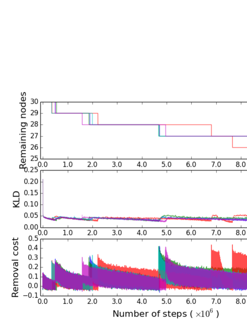
Figure 3: The number of hidden units $N$ (top), KLD (middle), and smallest removal cost (bottom) are shown as functions of the number of removal steps. The $3\times 3$ Bars-and-Stripes dataset was employed. PCD-5 was used for block Gibbs sampling. Each color corresponds to a different trial.

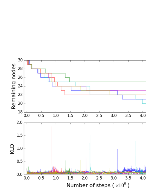
Figure 4: The number of hidden units $N$ (top), and KLD (bottom) are shown as functions of the number of removal steps. The $3\times 3$ Bars-and-Stripes dataset was employed. PCD-1 was used for block Gibbs sampling. Each color corresponds to a different trial.

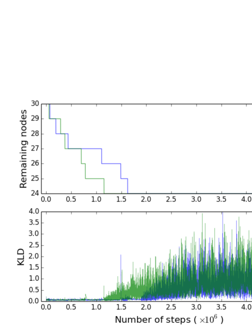
Figure 5: Two trials failed to keep the KLD in case of the PCD-1. Large fluctuations of the KLD appear immediately (green) and sufficiently (blue) after node removal.

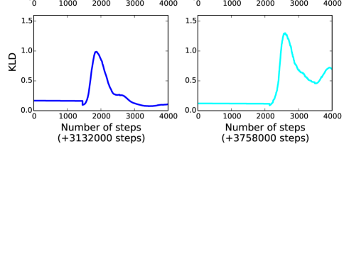
Figure 6: The peaks after the $3,000,000$th step (blue line) and before the $4,000,000$th step (cyan line) in Figure 4 are enlarged. These figures show that node removal slightly decreases the KLD, and parameter updates immediately following removal caused increases in the KLD.

4.2 MNIST

We used $60,000$ out of $70,000$ MNIST images for the evaluation of $C_{k}\,$, $\nabla_{\boldsymbol{\xi}}C_{k}\,$, and $\nabla_{\boldsymbol{\xi}}D$ in the learning and removal processes. Each pixel value was probabilistically set to $1$ proportional to its intensity (Salakhutdinov  Murray (2008); Tieleman (2008)). We first trained the RBM with $M=784$ visible units and $N=500$ hidden units using PCD-1 with a batch size of $1,000$ and fixed learning rate $\lambda=10^{-2}\,$. After $200,000$ learning steps, we performed the removal processes starting from the same trained RBM with a batch size of $1,000$ and a fixed parameter change rate, $\nu=10^{-2}\,$. In this case, the typical value of $\overline{\sigma_{C^{\prime}_{k}}}/D$ at the first removal step is small, that is, $\overline{\sigma_{C^{\prime}_{k}}}/D\sim 10^{-4}\,$. Thus, we employed $\overline{C_{k}^{\prime}}+\overline{\sigma_{C^{\prime}_{k}}}\leq 0$ as the removal criterion in order to quickly remove hidden units under the restriction that they do not drastically decrease the performance.

As mentioned in section 2, the KLD cannot be evaluated, owing to unknown probability $q({\boldsymbol{v}})$ and a large state space of the RBM. Thus, we employed an alternative evaluation criterion, namely, the KLD of $p({\boldsymbol{v}})$ from empirical distribution of samples generated from the test set, $q_{\rm d}({\boldsymbol{v}})\,$,

$$\widetilde{D} \equiv D_{\rm KL}({q_{\rm d}}||{p})$$ (28)

$$= \sum_{\boldsymbol{v}}q_{\rm d}({\boldsymbol{v}})\,\ln q_{\rm d}({\boldsymbol{v}})+\ln Z$$

$$+\sum_{\boldsymbol{v}}q_{\rm d}({\boldsymbol{v}})\,\left[\sum_{i}b_{i}\,v_{i}+\sum_{j}\ln\left(1+{\rm e}^{c_{j}+\sum_{i}v_{i}\,w_{ij}}\right)\right]\,,$$

where $Z$ is the normalization constant of $p({\boldsymbol{v}})$ and was evaluated by annealed importance sampling (AIS) (Neal (2001)). In the AIS, we used $100$ samples and linearly divided the inverse temperature from $\beta=0$ to $\beta=1$ into $10,000$ intervals. Since the evaluation of $Z$ by AIS takes a long time, we calculated $\widetilde{D}$ at every $50,000$ step. Between the intervals of evaluations of $\widetilde{D}\,$, we employed another evaluation criterion, the reconstruction error, for reference. The reconstruction error, $R\,$, can be easily calculated and is widely used to roughly estimate the performance of the RBM (Bengio . (2007); Taylor . (2007); Hinton (2012)):

$$R = -\frac{1}{S}\,\sum_{\alpha=1}^{S}\sum_{i=1}^{M}\left[v_{i}^{\alpha}\,\ln\widetilde{v}_{i}^{\alpha}+(1-v_{i}^{\alpha})\,\ln(1-\widetilde{v}_{i}^{\alpha})\right]\,,$$ (29)

$$\widetilde{v}_{i}^{\alpha} = \frac{{\rm e}^{b_{i}+\sum_{j}w_{ij}\widetilde{h}_{j}^{\alpha}}}{1+{\rm e}^{b_{i}+\sum_{j}w_{ij}\widetilde{h}_{j}^{\alpha}}}\,,$$ (30)

$$\widetilde{h}_{j}^{\alpha} = \frac{{\rm e}^{c_{j}+\sum_{i}v_{i}^{\alpha}w_{ij}}}{1+{\rm e}^{c_{j}+\sum_{i}v_{i}^{\alpha}w_{ij}}}\,,$$ (31)

where $\alpha$ denotes the index of a mini-batch, and ${\boldsymbol{v}}^{\alpha}$ is a sample from the training set.

The progress of the removal processes is shown in Figure 7, and samples of visible variables at the beginning and the end of the removal processes are presented in Figure 8. From the behavior of $N\,$, $\widetilde{D}\,$, and $R$ in Figure 7, it can be found that in a realistic-size RBM, our algorithm decreases the number of hidden units while avoiding a drastic increase in the KLD . We stopped three removal processes after $800,000$ steps, and the RBMs were compressed to $N\sim 400\,$. The number of removal steps is much larger than that of the learning steps. However, this is not a defect of our algorithm, since our motivation is not to quickly compress the RBM but to preserve its performance during the removal process. As a reference for the performance of the compressed RBMs, we trained the RBM with $N=400$ using the same setting employed in the learning of the RBM with $N=500\,$. The performance of this RBM was $\widetilde{D}=78.0\pm 0.3$ (where $\pm$ indicates $1\sigma$ confidence interval), which is almost the same performance of the RBMs after the removal process. This result suggests that our algorithm does not harm the performance, although we did not highly optimize the learning process for the RBMs with $N=400$ and $N=500\,$. The gradual increase of the upper side of $C^{\prime}_{k}$ in Figure 7 supports our intuitive explanation that the contribution of the remaining hidden units to the performance increases in order to maintain the performance. Thus, also in this case, an extremely long removal process can increase $|{\boldsymbol{\xi}}|$ and may lead to failure of Gibbs sampling. Thus, the removal process should be stopped before a successive increase in the KLD occurs. Since the KLD cannot be evaluated in large-size RBMs, we recommend monitoring the change in performance by employing some evaluation criterion used in the learning process in previous studies, e.g. the reconstruction error (Bengio . (2007); Taylor . (2007); Hinton (2012)), the product of the two probabilities ratio (Buchaca . (2013)), and the likelihood of a validation set obtained by tracking the partition functions (Desjardins . (2011)) .

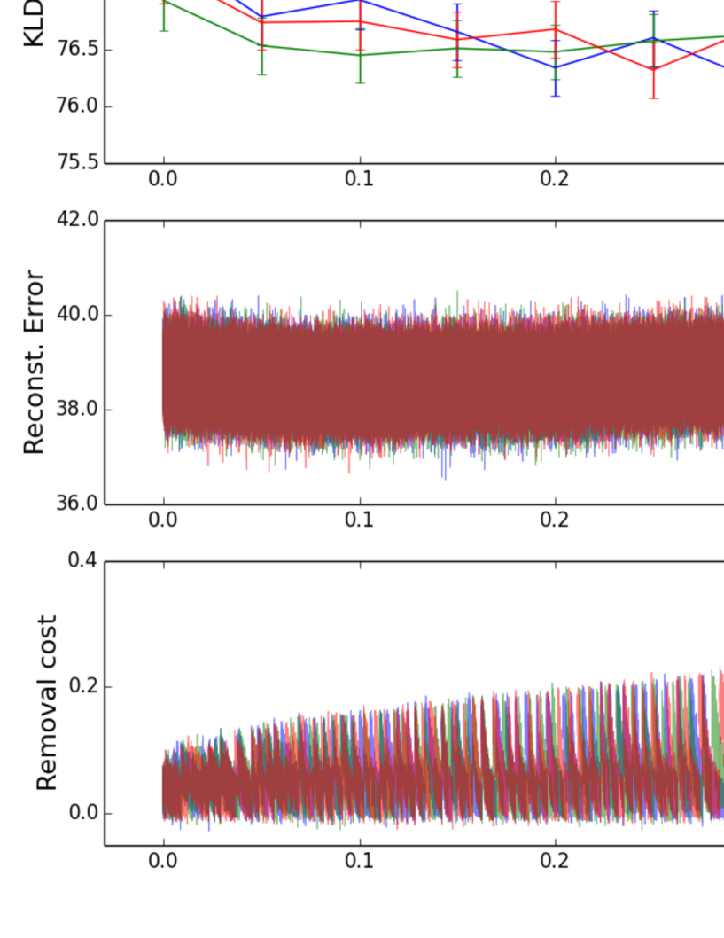
Figure 7: From the top to the bottom, the number of hidden units $N\,$, the KLD of $p({\boldsymbol{v}})$ from $q_{\rm d}({\boldsymbol{v}})\,$, the reconstruction error $R\,$, and the effective removal cost are shown as functions of the number of removal steps. MNIST handwritten images were employed as the dataset. Each color corresponds to a different trial. In the second panel from the top, the width of the KLD represents $1\sigma$ confidence intervals, and the negative log-likelihood (NLL), $-l\equiv\widetilde{D}-\sum_{\boldsymbol{v}}q_{\rm d}({\boldsymbol{v}})\,\ln q_{\rm d}({\boldsymbol{v}})\,$, is also shown for the evaluation of the performance together with $\widetilde{D}\,$.

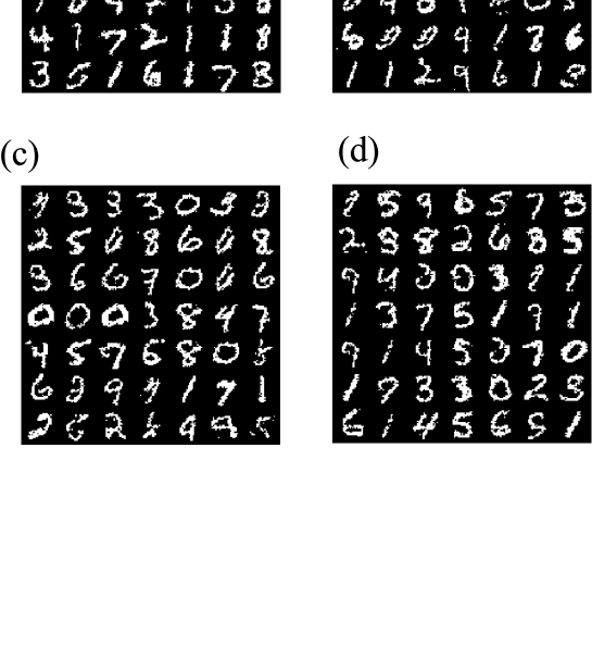
Figure 8: MNIST images are shown at the start and ends of the removal processes. (a) Samples of visible configurations at the $0$th step of the removal processes. (b, c, d) Samples of visible configurations at the $800,000$th step of the blue, green, and red lines in Figure 7, respectively.

5 Summary and discussion

In this paper, we aimed to decrease the number of hidden units of the RBM without affecting its performance. For this purpose, we have introduced the removal cost of a hidden unit and have proposed a method to remove it while avoiding a drastic increase in the KLD. Then, we have applied the proposed method to two different datasets and have shown that the KLD was approximately maintained during the removal processes. The increase in the KLD observed in the numerical simulations was caused by the failure of Gibbs sampling, which is also a problem in the learning process. The RBM has been facing difficulties such as accurately obtaining expectation values that are computationally expensive. Several kinds of Gibbs sampling methods have been proposed (Hinton (2002); Tieleman (2008); Tieleman  Hinton (2009); Salakhutdinov (2009); Cho . (2010); Desjardins . (2010)), which provide precise estimates and increase the performance of the RBM. However, more accurate Gibbs sampling methods require a longer time for evaluations. If expectation values can be precisely evaluated, then our algorithm is expected be more effective. We expect that physical implementation of the RBM (Dumoulin . (2014)) becomes an accurate and fast method for their evaluation.

Finally, we comment on another application of the removal cost. If the representational power of the system is sufficient, then an arbitrary hidden unit can be safely removed by decreasing its removal cost. Hence, by repeatedly adding and removing hidden units, entire hidden units of a system can be replaced. Such a procedure may be useful for reforming physically implemented systems that are difficult to copy and must not be halted.

6 Acknowledgment

This research is supported by JSPS KAKENHI Grant Number 15H00800.

Appendix A Derivation of Eq. (13)

For convenience, we introduce two unnormalized probabilities, $p^{*}({\boldsymbol{v}},{\boldsymbol{h}})={\rm e}^{-E({\boldsymbol{v}},{\boldsymbol{h}})}$ and $p^{*}_{\backslash k}({\boldsymbol{v}},{\boldsymbol{h}}_{\backslash k})={\rm e}^{-E({\boldsymbol{v}},{\boldsymbol{h}})}|_{h_{k}=0}\,$. Then, we can obtain $C_{k}$ as follows:

$$C_{k} = D_{\rm KL}({q}||{p_{\backslash k}})-D_{\rm KL}({q}||{p})$$ (32)

$$= \sum_{\boldsymbol{v}}q({\boldsymbol{v}})\,\ln\frac{q({\boldsymbol{v}})}{\sum_{{\boldsymbol{h}}_{\backslash k}}p_{\backslash k}({\boldsymbol{v}},{\boldsymbol{h}}_{\backslash k})}-\sum_{\boldsymbol{v}}q({\boldsymbol{v}})\,\ln\frac{q({\boldsymbol{v}})}{\sum_{\boldsymbol{h}}p({\boldsymbol{v}},{\boldsymbol{h}})}$$

$$= -\sum_{\boldsymbol{v}}q({\boldsymbol{v}})\,\ln\sum_{{\boldsymbol{h}}_{\backslash k}}p_{\backslash k}({\boldsymbol{v}},{\boldsymbol{h}}_{\backslash k})+\sum_{\boldsymbol{v}}q({\boldsymbol{v}})\,\ln\sum_{\boldsymbol{h}}p({\boldsymbol{v}},{\boldsymbol{h}})$$

$$= -\sum_{\boldsymbol{v}}q({\boldsymbol{v}})\,\ln\frac{\sum_{{\boldsymbol{h}}_{\backslash k}}p_{\backslash k}^{*}({\boldsymbol{v}},{\boldsymbol{h}}_{\backslash k})}{\sum_{{\boldsymbol{v}}^{\prime},{\boldsymbol{h}}^{\prime}_{\backslash k}}p_{\backslash k}^{*}({\boldsymbol{v}}^{\prime},{\boldsymbol{h}}^{\prime}_{\backslash k})}+\sum_{\boldsymbol{v}}q({\boldsymbol{v}})\,\ln\frac{\sum_{\boldsymbol{h}}p^{*}({\boldsymbol{v}},{\boldsymbol{h}})}{\sum_{{\boldsymbol{v}}^{\prime},{\boldsymbol{h}}^{\prime}}p^{*}({\boldsymbol{v}}^{\prime},{\boldsymbol{h}}^{\prime})}$$

$$= -\sum_{\boldsymbol{v}}q({\boldsymbol{v}})\,\ln\frac{\sum_{{\boldsymbol{h}}_{\backslash k}}p^{*}({\boldsymbol{v}},{\boldsymbol{h}})|_{h_{k}=0}}{\sum_{{\boldsymbol{v}}^{\prime},{\boldsymbol{h}}^{\prime}_{\backslash k}}p^{*}({\boldsymbol{v}}^{\prime},{\boldsymbol{h}}^{\prime})|_{h_{k}=0}}+\sum_{\boldsymbol{v}}q({\boldsymbol{v}})\,\ln\frac{\sum_{\boldsymbol{h}}p^{*}({\boldsymbol{v}},{\boldsymbol{h}})}{\sum_{{\boldsymbol{v}}^{\prime},{\boldsymbol{h}}^{\prime}}p^{*}({\boldsymbol{v}}^{\prime},{\boldsymbol{h}}^{\prime})}$$

$$= -\sum_{\boldsymbol{v}}q({\boldsymbol{v}})\,\ln\frac{\sum_{{\boldsymbol{h}}_{\backslash k}}p^{*}({\boldsymbol{v}},{\boldsymbol{h}})|_{h_{k}=0}}{\sum_{\boldsymbol{h}}p^{*}({\boldsymbol{v}},{\boldsymbol{h}})}+\ln\frac{\sum_{{\boldsymbol{v}}^{\prime},{\boldsymbol{h}}^{\prime}_{\backslash k}}p^{*}({\boldsymbol{v}}^{\prime},{\boldsymbol{h}}^{\prime})|_{h_{k}=0}}{\sum_{{\boldsymbol{v}}^{\prime},{\boldsymbol{h}}^{\prime}}p^{*}({\boldsymbol{v}}^{\prime},{\boldsymbol{h}}^{\prime})}$$

$$= -\sum_{\boldsymbol{v}}q({\boldsymbol{v}})\,\ln p(h_{k}=0|{\boldsymbol{v}})+\ln p(h_{k}=0)\,.$$

Next, consider the simultaneous removal of several hidden units. Suppose ${}^{t}\!{\boldsymbol{k}}=(k_{1},\ldots,k_{r})$ denotes the indices of the hidden units to be removed and define $p_{\backslash{\boldsymbol{k}}}({\boldsymbol{v}})$ as the probability distribution after removal of these hidden units. Following a similar calculation above, we obtain the removal cost for several hidden units:

$$C_{\boldsymbol{k}} \equiv D_{\rm KL}({q}||{p_{\backslash{\boldsymbol{k}}}})-D_{\rm KL}({q}||{p})$$ (33)

$$= -\sum_{\boldsymbol{v}}q({\boldsymbol{v}})\,\ln p(h_{k_{1}}=\cdots=h_{k_{r}}=0|{\boldsymbol{v}})$$

$$+\ln p(h_{k_{1}}=\cdots=h_{k_{r}}=0)\,.$$

In the case of the RBM, the first term of Eq. (33) can be simplified as

$$C_{\boldsymbol{k}} = D_{\rm KL}({q}||{p_{\backslash{\boldsymbol{k}}}})-D_{\rm KL}({q}||{p})$$ (34)

$$= -\sum_{\boldsymbol{v}}q({\boldsymbol{v}})\,\sum_{\alpha=1}^{r}\ln p(h_{k_{\alpha}}=0|{\boldsymbol{v}})$$

$$+\ln p(h_{k_{1}}=\cdots=h_{k_{r}}=0)\,.$$

This removal cost can be used to minimize the size of the RBM. Suppose $D_{0}$ is the KLD to be preserved. If some set of parameters, ${\boldsymbol{\xi}}\,$, satisfies $C_{\boldsymbol{k}}=0$ and $D=D_{0}\,$, then the hidden units whose indices are ${\boldsymbol{k}}$ can be removed simultaneously without changing the KLD. Furthermore, if one can find a set ${\boldsymbol{\xi}}$ that can remove as many hidden units as as possible, then the size of the RBM is minimized. However, finding such a set of parameters is difficult problem.

Appendix B Change of $D$ and $C_{k}$ by the naive update rule, Eq. (14)

In this Appendix, we show that the naive update rule, Eq. (14), decreases both $D$ and $C_{k}$ at ${\cal O}(|\Delta{\boldsymbol{\xi}}|)\,$. The change of $D$ and $C_{k}$ by Eq. (14) at ${\cal O}(|\Delta{\boldsymbol{\xi}}|)$ are given by

$$\frac{\partial D}{\partial\xi_{i}}\,\Delta\xi_{i} = -\nu\cdot\theta\left(\frac{\partial D}{\partial\xi_{i}}\,\frac{\partial C_{k}}{\partial\xi_{i}}\right)\cdot\left(\frac{\partial D}{\partial\xi_{i}}\right)^{2}\,,$$ (35)

$$\frac{\partial C_{k}}{\partial\xi_{i}}\,\Delta\xi_{i} = -\nu\cdot\theta\left(\frac{\partial D}{\partial\xi_{i}}\,\frac{\partial C_{k}}{\partial\xi_{i}}\right)\cdot\frac{\partial D}{\partial\xi_{i}}\cdot\frac{\partial C_{k}}{\partial\xi_{i}}\,.$$ (36)

In the case of $\partial D/\partial\xi_{i}\cdot\partial C_{k}/\partial\xi_{i}\geq 0\,$, Eq. (35) and Eq. (36) become

$$\frac{\partial D}{\partial\xi_{i}}\,\Delta\xi_{i} = -\nu\cdot\left(\frac{\partial D}{\partial\xi_{i}}\right)^{2}\leq 0\,,$$ (37)

$$\frac{\partial C_{k}}{\partial\xi_{i}}\,\Delta\xi_{i} = -\nu\cdot\frac{\partial D}{\partial\xi_{i}}\cdot\frac{\partial C_{k}}{\partial\xi_{i}}\leq 0\,,$$ (38)

and in the case of $\partial D/\partial\xi_{i}\cdot\partial C_{k}/\partial\xi_{i}<0\,$, Eq. (35) and Eq. (36) become

$$\frac{\partial D}{\partial\xi_{i}}\,\Delta\xi_{i} = 0\,,$$ (39)

$$\frac{\partial C_{k}}{\partial\xi_{i}}\,\Delta\xi_{i} = 0\,.$$ (40)

In both cases, Eq. (35) and Eq. (36) take non-positive values. Thus, this update rule decreases both $D$ and $C_{k}$ at ${\cal O}(|\Delta{\boldsymbol{\xi}}|)\,$.

References

- Ackley \BOthers. (\APACyear1987) \APACinsertmetastarackley1987learning{APACrefauthors}Ackley, D\BPBIH., Hinton, G\BPBIE.\BCBL \BBA Sejnowski, T\BPBIJ. \APACrefYearMonthDay1987. \BBOQ\APACrefatitleA learning algorithm for Boltzmann machines A learning algorithm for boltzmann machines.\BBCQ \BIn \APACrefbtitleReadings in Computer Vision Readings in computer vision (\BPGS 522–533). \APACaddressPublisherElsevier. \PrintBackRefs\CurrentBib
- Bengio \BOthers. (\APACyear2013) \APACinsertmetastarbengio2013representation{APACrefauthors}Bengio, Y., Courville, A.\BCBL \BBA Vincent, P. \APACrefYearMonthDay2013. \BBOQ\APACrefatitleRepresentation learning: A review and new perspectives Representation learning: A review and new perspectives.\BBCQ \APACjournalVolNumPagesIEEE transactions on pattern analysis and machine intelligence3581798–1828. \PrintBackRefs\CurrentBib
- Bengio \BOthers. (\APACyear2007) \APACinsertmetastarbengio2007greedy{APACrefauthors}Bengio, Y., Lamblin, P., Popovici, D.\BCBL \BBA Larochelle, H. \APACrefYearMonthDay2007. \BBOQ\APACrefatitleGreedy layer-wise training of deep networks Greedy layer-wise training of deep networks.\BBCQ \BIn \APACrefbtitleAdvances in neural information processing systems Advances in neural information processing systems (\BPGS 153–160). \PrintBackRefs\CurrentBib
- Berglund \BOthers. (\APACyear2015) \APACinsertmetastarberglund2015measuring{APACrefauthors}Berglund, M., Raiko, T.\BCBL \BBA Cho, K. \APACrefYearMonthDay2015. \BBOQ\APACrefatitleMeasuring the usefulness of hidden units in Boltzmann machines with mutual information Measuring the usefulness of hidden units in boltzmann machines with mutual information.\BBCQ \APACjournalVolNumPagesNeural Networks6412–18. \PrintBackRefs\CurrentBib
- Buchaca \BOthers. (\APACyear2013) \APACinsertmetastarbuchaca2013stopping{APACrefauthors}Buchaca, D., Romero, E., Mazzanti, F.\BCBL \BBA Delgado, J. \APACrefYearMonthDay2013. \BBOQ\APACrefatitleStopping criteria in contrastive divergence: Alternatives to the reconstruction error Stopping criteria in contrastive divergence: Alternatives to the reconstruction error.\BBCQ \APACjournalVolNumPagesarXiv preprint arXiv:1312.6062. \PrintBackRefs\CurrentBib
- Carleo \BBA Troyer (\APACyear2017) \APACinsertmetastarcarleo2017solving{APACrefauthors}Carleo, G.\BCBT \BBA Troyer, M. \APACrefYearMonthDay2017. \BBOQ\APACrefatitleSolving the quantum many-body problem with artificial neural networks Solving the quantum many-body problem with artificial neural networks.\BBCQ \APACjournalVolNumPagesScience3556325602–606. \PrintBackRefs\CurrentBib
- Cheng \BOthers. (\APACyear2017) \APACinsertmetastarcheng2017survey{APACrefauthors}Cheng, Y., Wang, D., Zhou, P.\BCBL \BBA Zhang, T. \APACrefYearMonthDay2017. \BBOQ\APACrefatitleA Survey of Model Compression and Acceleration for Deep Neural Networks A survey of model compression and acceleration for deep neural networks.\BBCQ \APACjournalVolNumPagesarXiv preprint arXiv:1710.09282. \PrintBackRefs\CurrentBib
- Cho \BOthers. (\APACyear2010) \APACinsertmetastarcho2010parallel{APACrefauthors}Cho, K., Raiko, T.\BCBL \BBA Ilin, A. \APACrefYearMonthDay2010. \BBOQ\APACrefatitleParallel tempering is efficient for learning restricted Boltzmann machines Parallel tempering is efficient for learning restricted boltzmann machines.\BBCQ \BIn \APACrefbtitleNeural Networks (IJCNN), The 2010 International Joint Conference on Neural networks (ijcnn), the 2010 international joint conference on (\BPGS 1–8). \PrintBackRefs\CurrentBib
- Christopher (\APACyear2016) \APACinsertmetastarchristopher2016pattern{APACrefauthors}Christopher, M\BPBIB. \APACrefYear2016. \APACrefbtitlePATTERN RECOGNITION AND MACHINE LEARNING. Pattern recognition and machine learning. \APACaddressPublisherSpringer-Verlag New York. \PrintBackRefs\CurrentBib
- Desjardins \BOthers. (\APACyear2011) \APACinsertmetastardesjardins2011tracking{APACrefauthors}Desjardins, G., Bengio, Y.\BCBL \BBA Courville, A\BPBIC. \APACrefYearMonthDay2011. \BBOQ\APACrefatitleOn tracking the partition function On tracking the partition function.\BBCQ \BIn \APACrefbtitleAdvances in neural information processing systems Advances in neural information processing systems (\BPGS 2501–2509). \PrintBackRefs\CurrentBib
- Desjardins \BOthers. (\APACyear2010) \APACinsertmetastardesjardins2010tempered{APACrefauthors}Desjardins, G., Courville, A., Bengio, Y., Vincent, P.\BCBL \BBA Delalleau, O. \APACrefYearMonthDay2010. \BBOQ\APACrefatitleTempered Markov chain Monte Carlo for training of restricted Boltzmann machines Tempered markov chain monte carlo for training of restricted boltzmann machines.\BBCQ \BIn \APACrefbtitleProceedings of the thirteenth international conference on artificial intelligence and statistics Proceedings of the thirteenth international conference on artificial intelligence and statistics (\BPGS 145–152). \PrintBackRefs\CurrentBib
- Dumoulin \BOthers. (\APACyear2014) \APACinsertmetastardumoulin2014challenges{APACrefauthors}Dumoulin, V., Goodfellow, I\BPBIJ., Courville, A\BPBIC.\BCBL \BBA Bengio, Y. \APACrefYearMonthDay2014. \BBOQ\APACrefatitleOn the Challenges of Physical Implementations of RBMs. On the challenges of physical implementations of rbms.\BBCQ \BIn \APACrefbtitleAAAI Aaai (\BVOL 2014, \BPGS 1199–1205). \PrintBackRefs\CurrentBib
- Fischer \BBA Igel (\APACyear2010) \APACinsertmetastarfischer2010empirical{APACrefauthors}Fischer, A.\BCBT \BBA Igel, C. \APACrefYearMonthDay2010. \BBOQ\APACrefatitleEmpirical analysis of the divergence of Gibbs sampling based learning algorithms for restricted Boltzmann machines Empirical analysis of the divergence of gibbs sampling based learning algorithms for restricted boltzmann machines.\BBCQ \BIn \APACrefbtitleInternational Conference on Artificial Neural Networks International conference on artificial neural networks (\BPGS 208–217). \PrintBackRefs\CurrentBib
- Fischer \BBA Igel (\APACyear2012) \APACinsertmetastarfischer2012introduction{APACrefauthors}Fischer, A.\BCBT \BBA Igel, C. \APACrefYearMonthDay2012. \BBOQ\APACrefatitleAn introduction to restricted Boltzmann machines An introduction to restricted boltzmann machines.\BBCQ \BIn \APACrefbtitleIberoamerican Congress on Pattern Recognition Iberoamerican congress on pattern recognition (\BPGS 14–36). \PrintBackRefs\CurrentBib
- Goodfellow \BOthers. (\APACyear2014) \APACinsertmetastargoodfellow2014generative{APACrefauthors}Goodfellow, I., Pouget-Abadie, J., Mirza, M., Xu, B., Warde-Farley, D., Ozair, S.\BDBLBengio, Y. \APACrefYearMonthDay2014. \BBOQ\APACrefatitleGenerative adversarial nets Generative adversarial nets.\BBCQ \BIn \APACrefbtitleAdvances in neural information processing systems Advances in neural information processing systems (\BPGS 2672–2680). \PrintBackRefs\CurrentBib
- Guo \BOthers. (\APACyear2016) \APACinsertmetastarguo2016dynamic{APACrefauthors}Guo, Y., Yao, A.\BCBL \BBA Chen, Y. \APACrefYearMonthDay2016. \BBOQ\APACrefatitleDynamic network surgery for efficient dnns Dynamic network surgery for efficient dnns.\BBCQ \BIn \APACrefbtitleAdvances In Neural Information Processing Systems Advances in neural information processing systems (\BPGS 1379–1387). \PrintBackRefs\CurrentBib
- Han \BOthers. (\APACyear2015) \APACinsertmetastarhan2015learning{APACrefauthors}Han, S., Pool, J., Tran, J.\BCBL \BBA Dally, W. \APACrefYearMonthDay2015. \BBOQ\APACrefatitleLearning both weights and connections for efficient neural network Learning both weights and connections for efficient neural network.\BBCQ \BIn \APACrefbtitleAdvances in neural information processing systems Advances in neural information processing systems (\BPGS 1135–1143). \PrintBackRefs\CurrentBib
- He \BOthers. (\APACyear2016) \APACinsertmetastarhe2016deep{APACrefauthors}He, K., Zhang, X., Ren, S.\BCBL \BBA Sun, J. \APACrefYearMonthDay2016. \BBOQ\APACrefatitleDeep residual learning for image recognition Deep residual learning for image recognition.\BBCQ \BIn \APACrefbtitleProceedings of the IEEE conference on computer vision and pattern recognition Proceedings of the ieee conference on computer vision and pattern recognition (\BPGS 770–778). \PrintBackRefs\CurrentBib
- Hestness \BOthers. (\APACyear2017) \APACinsertmetastarhestness2017deep{APACrefauthors}Hestness, J., Narang, S., Ardalani, N., Diamos, G., Jun, H., Kianinejad, H.\BDBLZhou, Y. \APACrefYearMonthDay2017. \BBOQ\APACrefatitleDeep Learning Scaling is Predictable, Empirically Deep learning scaling is predictable, empirically.\BBCQ \APACjournalVolNumPagesarXiv preprint arXiv:1712.00409. \PrintBackRefs\CurrentBib
- Hinton (\APACyear2002) \APACinsertmetastarhinton2002training{APACrefauthors}Hinton, G\BPBIE. \APACrefYearMonthDay2002. \BBOQ\APACrefatitleTraining products of experts by minimizing contrastive divergence Training products of experts by minimizing contrastive divergence.\BBCQ \APACjournalVolNumPagesNeural computation1481771–1800. \PrintBackRefs\CurrentBib
- Hinton (\APACyear2012) \APACinsertmetastarhinton2012practical{APACrefauthors}Hinton, G\BPBIE. \APACrefYearMonthDay2012. \BBOQ\APACrefatitleA practical guide to training restricted Boltzmann machines A practical guide to training restricted boltzmann machines.\BBCQ \BIn \APACrefbtitleNeural networks: Tricks of the trade Neural networks: Tricks of the trade (\BPGS 599–619). \APACaddressPublisherSpringer. \PrintBackRefs\CurrentBib
- Hinton \BOthers. (\APACyear2006) \APACinsertmetastarhinton2006fast{APACrefauthors}Hinton, G\BPBIE., Osindero, S.\BCBL \BBA Teh, Y\BHBIW. \APACrefYearMonthDay2006. \BBOQ\APACrefatitleA fast learning algorithm for deep belief nets A fast learning algorithm for deep belief nets.\BBCQ \APACjournalVolNumPagesNeural computation1871527–1554. \PrintBackRefs\CurrentBib
- Hinton \BBA Salakhutdinov (\APACyear2006) \APACinsertmetastarhinton2006reducing{APACrefauthors}Hinton, G\BPBIE.\BCBT \BBA Salakhutdinov, R\BPBIR. \APACrefYearMonthDay2006. \BBOQ\APACrefatitleReducing the dimensionality of data with neural networks Reducing the dimensionality of data with neural networks.\BBCQ \APACjournalVolNumPagesscience3135786504–507. \PrintBackRefs\CurrentBib
- Larochelle \BBA Bengio (\APACyear2008) \APACinsertmetastarlarochelle2008classification{APACrefauthors}Larochelle, H.\BCBT \BBA Bengio, Y. \APACrefYearMonthDay2008. \BBOQ\APACrefatitleClassification using discriminative restricted Boltzmann machines Classification using discriminative restricted boltzmann machines.\BBCQ \BIn \APACrefbtitleProceedings of the 25th international conference on Machine learning Proceedings of the 25th international conference on machine learning (\BPGS 536–543). \PrintBackRefs\CurrentBib
- LeCun \BBA Cortes (\APACyear1998) \APACinsertmetastarlecun1998mnist{APACrefauthors}LeCun, Y.\BCBT \BBA Cortes, C. \APACrefYearMonthDay1998. \BBOQ\APACrefatitleThe MNIST database of handwritten digits The mnist database of handwritten digits.\BBCQ \APACjournalVolNumPageshttp://yann. lecun. com/exdb/mnist/. \PrintBackRefs\CurrentBib
- Le Roux \BBA Bengio (\APACyear2008) \APACinsertmetastarle2008representational{APACrefauthors}Le Roux, N.\BCBT \BBA Bengio, Y. \APACrefYearMonthDay2008. \BBOQ\APACrefatitleRepresentational power of restricted Boltzmann machines and deep belief networks Representational power of restricted boltzmann machines and deep belief networks.\BBCQ \APACjournalVolNumPagesNeural computation2061631–1649. \PrintBackRefs\CurrentBib
- MacKay \BBA Mac Kay (\APACyear2003) \APACinsertmetastarmackay2003information{APACrefauthors}MacKay, D\BPBIJ.\BCBT \BBA Mac Kay, D\BPBIJ. \APACrefYear2003. \APACrefbtitleInformation theory, inference and learning algorithms Information theory, inference and learning algorithms. \APACaddressPublisherCambridge university press. \PrintBackRefs\CurrentBib
- Neal (\APACyear1996) \APACinsertmetastarneal1996sampling{APACrefauthors}Neal, R\BPBIM. \APACrefYearMonthDay1996. \BBOQ\APACrefatitleSampling from multimodal distributions using tempered transitions Sampling from multimodal distributions using tempered transitions.\BBCQ \APACjournalVolNumPagesStatistics and computing64353–366. \PrintBackRefs\CurrentBib
- Neal (\APACyear2001) \APACinsertmetastarneal2001annealed{APACrefauthors}Neal, R\BPBIM. \APACrefYearMonthDay2001. \BBOQ\APACrefatitleAnnealed importance sampling Annealed importance sampling.\BBCQ \APACjournalVolNumPagesStatistics and computing112125–139. \PrintBackRefs\CurrentBib
- Oord \BOthers. (\APACyear2016) \APACinsertmetastaroord2016wavenet{APACrefauthors}Oord, A\BPBIv\BPBId., Dieleman, S., Zen, H., Simonyan, K., Vinyals, O., Graves, A.\BDBLKavukcuoglu, K. \APACrefYearMonthDay2016. \BBOQ\APACrefatitleWavenet: A generative model for raw audio Wavenet: A generative model for raw audio.\BBCQ \APACjournalVolNumPagesarXiv preprint arXiv:1609.03499. \PrintBackRefs\CurrentBib
- Salakhutdinov (\APACyear2009) \APACinsertmetastarsalakhutdinov2009learning{APACrefauthors}Salakhutdinov, R. \APACrefYearMonthDay2009. \BBOQ\APACrefatitleLearning in Markov random fields using tempered transitions Learning in markov random fields using tempered transitions.\BBCQ \BIn \APACrefbtitleAdvances in neural information processing systems Advances in neural information processing systems (\BPGS 1598–1606). \PrintBackRefs\CurrentBib
- Salakhutdinov \BBA Hinton (\APACyear2009) \APACinsertmetastarsalakhutdinov2009deep{APACrefauthors}Salakhutdinov, R.\BCBT \BBA Hinton, G\BPBIE. \APACrefYearMonthDay2009. \BBOQ\APACrefatitleDeep Boltzmann Machines. Deep boltzmann machines.\BBCQ \BIn \APACrefbtitleAISTATS Aistats (\BVOL 1, \BPG 3). \PrintBackRefs\CurrentBib
- Salakhutdinov \BBA Larochelle (\APACyear2010) \APACinsertmetastarsalakhutdinov2010efficient{APACrefauthors}Salakhutdinov, R.\BCBT \BBA Larochelle, H. \APACrefYearMonthDay2010. \BBOQ\APACrefatitleEfficient learning of deep Boltzmann machines Efficient learning of deep boltzmann machines.\BBCQ \BIn \APACrefbtitleProceedings of the thirteenth international conference on artificial intelligence and statistics Proceedings of the thirteenth international conference on artificial intelligence and statistics (\BPGS 693–700). \PrintBackRefs\CurrentBib
- Salakhutdinov \BBA Murray (\APACyear2008) \APACinsertmetastarsalakhutdinov2008quantitative{APACrefauthors}Salakhutdinov, R.\BCBT \BBA Murray, I. \APACrefYearMonthDay2008. \BBOQ\APACrefatitleOn the quantitative analysis of deep belief networks On the quantitative analysis of deep belief networks.\BBCQ \BIn \APACrefbtitleProceedings of the 25th international conference on Machine learning Proceedings of the 25th international conference on machine learning (\BPGS 872–879). \PrintBackRefs\CurrentBib
- Smolensky (\APACyear1986) \APACinsertmetastarsmolensky1986information{APACrefauthors}Smolensky, P. \APACrefYearMonthDay1986. \APACrefbtitleInformation processing in dynamical systems: Foundations of harmony theory Information processing in dynamical systems: Foundations of harmony theory \APACbVolEdTR\BTR. \APACaddressInstitutionCOLORADO UNIV AT BOULDER DEPT OF COMPUTER SCIENCE. \PrintBackRefs\CurrentBib
- Taylor \BOthers. (\APACyear2007) \APACinsertmetastartaylor2007modeling{APACrefauthors}Taylor, G\BPBIW., Hinton, G\BPBIE.\BCBL \BBA Roweis, S\BPBIT. \APACrefYearMonthDay2007. \BBOQ\APACrefatitleModeling human motion using binary latent variables Modeling human motion using binary latent variables.\BBCQ \BIn \APACrefbtitleAdvances in neural information processing systems Advances in neural information processing systems (\BPGS 1345–1352). \PrintBackRefs\CurrentBib
- Tieleman (\APACyear2008) \APACinsertmetastartieleman2008training{APACrefauthors}Tieleman, T. \APACrefYearMonthDay2008. \BBOQ\APACrefatitleTraining restricted Boltzmann machines using approximations to the likelihood gradient Training restricted boltzmann machines using approximations to the likelihood gradient.\BBCQ \BIn \APACrefbtitleProceedings of the 25th international conference on Machine learning Proceedings of the 25th international conference on machine learning (\BPGS 1064–1071). \PrintBackRefs\CurrentBib
- Tieleman \BBA Hinton (\APACyear2009) \APACinsertmetastartieleman2009using{APACrefauthors}Tieleman, T.\BCBT \BBA Hinton, G. \APACrefYearMonthDay2009. \BBOQ\APACrefatitleUsing fast weights to improve persistent contrastive divergence Using fast weights to improve persistent contrastive divergence.\BBCQ \BIn \APACrefbtitleProceedings of the 26th Annual International Conference on Machine Learning Proceedings of the 26th annual international conference on machine learning (\BPGS 1033–1040). \PrintBackRefs\CurrentBib
- Tubiana \BBA Monasson (\APACyear2017) \APACinsertmetastartubiana2017emergence{APACrefauthors}Tubiana, J.\BCBT \BBA Monasson, R. \APACrefYearMonthDay2017. \BBOQ\APACrefatitleEmergence of compositional representations in restricted Boltzmann machines Emergence of compositional representations in restricted boltzmann machines.\BBCQ \APACjournalVolNumPagesPhysical review letters11813138301. \PrintBackRefs\CurrentBib
- Vaswani \BOthers. (\APACyear2017) \APACinsertmetastarvaswani2017attention{APACrefauthors}Vaswani, A., Shazeer, N., Parmar, N., Uszkoreit, J., Jones, L., Gomez, A\BPBIN.\BDBLPolosukhin, I. \APACrefYearMonthDay2017. \BBOQ\APACrefatitleAttention is all you need Attention is all you need.\BBCQ \BIn \APACrefbtitleAdvances in Neural Information Processing Systems Advances in neural information processing systems (\BPGS 6000–6010). \PrintBackRefs\CurrentBib