Chandrasekhar and sub-Chandrasekhar models for the X-ray emission of Type Ia supernova remnants (I): Bulk properties

Abstract

Type Ia supernovae originate from the explosion of carbon-oxygen white dwarfs in binary systems, but the exact nature of their progenitors remains elusive. The bulk properties of Type Ia supernova remnants, such as the radius and the centroid energy of the Fe K$\alpha$ blend in the X-ray spectrum, are determined by the properties of the supernova ejecta and the ambient medium. We model the interaction between Chandrasekhar and sub-Chandrasekhar models for Type Ia supernova ejecta and a range of uniform ambient medium densities in one dimension up to an age of 5000 years. We generate synthetic X-ray spectra from these supernova remnant models and compare their bulk properties at different expansion ages with X-ray observations from Chandra and Suzaku. We find that our models can successfully reproduce the bulk properties of most observed remnants, suggesting that Type Ia SN progenitors do not modify their surroundings significantly on scales of a few pc, although more detailed models are required to establish quantitative limits on the density of any such surrounding circumstellar material. Ambient medium density and expansion age are the main contributors to the diversity of the bulk properties in our models. Chandrasekhar and sub-Chandrasekhar progenitors make similar predictions for the bulk remnant properties, but detailed fits to X-ray spectra have the power to discriminate explosion energetics and progenitor scenarios.

1 Introduction

Type Ia supernovae (SNe Ia) are the thermonuclear explosions of white dwarf (WD) stars that are destabilized by mass accretion from a close binary companion. They are important for a wide range of topics in astrophysics, e.g. galactic chemical evolution (Kobayashi et al., 2006; Andrews et al., 2016; Prantzos et al., 2018), studies of dark energy (Riess et al., 1998; Perlmutter et al., 1999) and constraints on $\Lambda$CDM parameters (Betoule et al., 2014; Rest et al., 2014). Yet, basic aspects of SN Ia physics, such as the nature of their stellar progenitors and the triggering mechanism for the thermonuclear runaway, still remain obscure. Most proposed scenarios for the progenitor systems of SNe Ia fall into two broad categories: the single degenerate (SD), where the WD companion is a nondegenerate star, and the double degenerate (DD), where the WD companion is another WD (see Wang & Han, 2012; Maoz et al., 2014; Livio & Mazzali, 2018; Soker, 2018; Wang, 2018, for recent reviews).

In the SD scenario, the WD accretes material from its companion over a relatively long timescale (t$\,{\sim}\,10^{6}$ years) and explodes when its mass approaches the Chandrasekhar limit M${}_{\rm{Ch}}\,{\simeq}\,1.4\,M_{\odot}$ (Nomoto et al., 1984; Thielemann et al., 1986; Hachisu et al., 1996; Han & Podsiadlowski, 2004). Conversely, in most DD scenarios, the WD becomes unstable after a merger or a collision on a dynamical timescale (Iben & Tutukov, 1984) and explodes with a mass that is not necessarily close to M_Ch  (e.g., Raskin et al., 2009; van Kerkwijk et al., 2010; Kushnir et al., 2013). In theory, distinguishing between SD and DD systems should be feasible, given that some observational probes are sensitive to the duration of the accretion process or to the total mass prior to the explosion (e.g., Badenes et al., 2007, 2008a; Seitenzahl et al., 2013; Margutti et al., 2014; Scalzo et al., 2014; Yamaguchi et al., 2015; Chomiuk et al., 2016; Martínez-Rodríguez et al., 2016).

Sub-Chandrasekhar models (e.g., Woosley & Weaver, 1994; Sim et al., 2010; Woosley & Kasen, 2011) are a particular subset of both SD and DD SN Ia progenitors. To first order, the mass of $\rm{{}^{56}Ni}$ synthesized, and therefore the brightness of the supernova, is determined by the mass of the exploding WD. A sub-M_Ch WD cannot detonate spontaneously without some kind of external compression – double-detonations are frequently invoked (e.g., Shen et al., 2013; Shen & Bildsten, 2014; Shen & Moore, 2014; Shen et al., 2018). Here, a carbon-oxygen (C/O) WD accretes material from a companion and develops a helium-rich layer that eventually becomes unstable, ignites, and sends a shock wave into the core. This blast wave converges and creates another shock that triggers a carbon denotation, which explodes the WD. Violent mergers (e.g., Pakmor et al., 2012, 2013) are an alternative scenario where, right before the secondary WD is disrupted, carbon burning starts on the surface of the primary WD and a detonation propagates through the whole merger, triggering a thermonuclear runaway. Other studies present pure detonations of sub-M_Ch C/O WDs with different masses without addressing the question of how they were initiated. However, these studies are still able to reproduce many observables such as light curves, nickel ejecta masses, and isotopic mass ratios (Sim et al., 2010; Piro et al., 2014; Yamaguchi et al., 2015; Blondin et al., 2017; Martínez-Rodríguez et al., 2017; Goldstein & Kasen, 2018; Shen et al., 2018).

After the light from the supernova (SN) fades away, the ejecta expand and cool down until their density becomes comparable to that of the ambient medium, either the interstellar medium (ISM) or a more or less extended circumstellar medium (CSM) modified by the SN progenitor. At this point, the supernova remnant (SNR) phase begins. The ejecta drive a blast wave into the ambient medium (“forward shock”, FS), and the pressure gradient creates another wave back into the ejecta (“reverse shock”, RS; McKee & Truelove, 1995; Truelove & McKee, 1999).

Table 1: Total yields for the sub-M_Ch and M_Ch progenitor models. See Bravo et al. (2018) for details and extended yields.

Progenitor $M_{\rm{C}}$ $M_{\rm{O}}$ $M_{\rm{Ne}}$ $M_{\rm{Mg}}$ $M_{\rm{Si}}$ $M_{\rm{S}}$ $M_{\rm{Ar}}$ $M_{\rm{Ca}}$ $M_{\rm{Cr}}$ $M_{\rm{Mn}}$ $M_{\rm{Fe}}$ $M_{\rm{Ni}}$ $(M_{\odot})$ $(M_{\odot})$ $(M_{\odot})$ $(M_{\odot})$ $(M_{\odot})$ $(M_{\odot})$ $(M_{\odot})$ $(M_{\odot})$ $(M_{\odot})$ $(M_{\odot})$ $(M_{\odot})$ $(M_{\odot})$ SCH088 3.95E-03 1.40E-01 2.54E-03 1.99E-02 2.79E-01 1.66E-01 3.70E-02 3.72E-02 6.90E-03 2.68E-03 1.82E-01 1.19E-03 SCH097 1.62E-03 7.66E-02 8.24E-04 7.80E-03 2.09E-01 1.36E-01 3.26E-02 3.52E-02 1.12E-02 4.24E-03 4.50E-01 3.18E-03 SCH106 6.91E-04 3.74E-02 2.80E-04 2.61E-03 1.38E-01 9.62E-02 2.39E-02 2.63E-02 9.11E-03 3.46E-03 7.01E-01 1.54E-02 SCH115 2.75E-04 1.47E-02 8.99E-05 6.34E-04 7.66E-02 5.66E-02 1.47E-02 1.66E-02 6.31E-03 2.40E-03 9.25E-01 2.71E-02 DDT12 4.88E-03 1.75E-01 3.88E-03 2.64E-02 3.84E-01 2.34E-01 5.29E-02 5.32E-02 1.50E-02 7.12E-03 3.84E-01 3.15E-02 DDT16 2.52E-03 1.19E-01 1.83E-03 1.55E-02 3.05E-01 1.98E-01 4.79E-02 5.20E-02 2.02E-02 8.76E-03 5.70E-01 3.16E-02 DDT24 1.26E-03 7.15E-02 7.06E-04 7.26E-03 2.10E-01 1.42E-01 3.54E-02 3.98E-02 2.20E-02 1.00E-02 8.00E-01 3.23E-02 DDT40 5.33E-04 3.80E-02 2.62E-04 2.88E-03 1.35E-01 9.43E-02 2.38E-02 2.66E-02 1.59E-02 7.51E-03 9.69E-01 5.03E-02

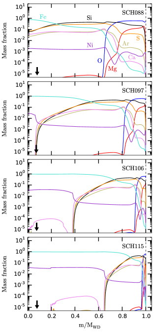
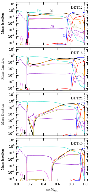
Figure 1: Chemical composition for our SN Ia models listed in Table 1. The vertical, dashed lines indicate the outer surface of each ejecta model. The arrows depict the locations of the RS at 538 years for $\rho_{\rm{amb}}\,=\,2\times 10^{-24}\,\rm{g\,cm^{-3}}$ (see the discussion in Section 2.3).

The X-ray emission from young (${\sim}$ a few 1000 years) SNRs is often-times dominated by strong emission lines from the shocked ejecta that can be used to probe the nucleosynthesis of the progenitor. These thermal (${\sim}\,10^{7}\,$K) X-ray spectra are as diverse as their SN progenitors, and not even remnants of similar ages are alike. Their evolution and properties depend on various factors such as the structure and composition of the ejecta, the energy of the explosion, and the structure of the CSM that is left behind by the progenitor (e.g., Badenes et al., 2003, 2007; Patnaude et al., 2012, 2017; Woods et al., 2017, 2018).

Therefore, young SNRs offer unique insights into both the supernova explosion and the structure of the ambient medium. They are excellent laboratories to study the SN phenomenon (e.g., Badenes et al., 2005, 2006, 2008b; Badenes, 2010; Vink, 2012; Lee et al., 2013, 2014, 2015; Slane et al., 2014; Patnaude et al., 2015). The X-ray spectra of SNRs, unlike the optical spectra of SNe Ia, allow us to explore these issues without having to consider the complexities of radiative transfer (e.g., Stehle et al., 2005; Tanaka et al., 2011; Ashall et al., 2016; Wilk et al., 2018), because the plasma is at low enough density to be optically thin to its own radiation.

It is known that M_Ch models interacting with a uniform ambient medium can successfully reproduce the bulk properties of SNRs, such as ionization timescales (Badenes et al., 2007), Fe K$\alpha$ centroid energies, Fe K$\alpha$ luminosities (Yamaguchi et al., 2014a), and radii (Patnaude & Badenes, 2017). However, there has been no exploration of the parameter space associated with the evolution of sub-M_Ch explosion models during the SNR stage for various dynamical ages. Here, we develop the first model grid of sub-M_Ch explosions in the SNR phase. We compare the bulk spectral and dynamical properties of M_Ch and sub-M_Ch models to the observed characteristics of Galactic and Magellanic Cloud Ia SNRs.

This paper is organized as follows. In Section 2, we describe our hydrodynamical SNR models and the derivation of synthetic X-ray spectra. In Section 3, we compare the bulk properties predicted by our model grid with observational data of Type Ia SNRs. Finally, in Section 4, we summarize our results and outline future analyses derived from our work.

2 Method

2.1 Supernova explosion models

We use the spherically symmetric M_Ch and sub-M_Ch explosion models introduced in Yamaguchi et al. (2015), Martínez-Rodríguez et al. (2017) and McWilliam et al. (2018), which are calculated with a version of the code described in Bravo & Martínez-Pinedo (2012), updated to account for an accurate coupling between hydrodynamics and nuclear reactions (Bravo et al., 2016, 2018). The M_Ch models are delayed detonations (Khokhlov, 1991) with a central density $\rho_{\rm{c}}=3\times 10^{9}\,\rm{g\,cm^{-3}}$, deflagration-to-detonation densities $\rho_{\rm{DDT}}$ $\rm{[10^{7}\,g\,cm^{-3}]}=$ $1.2,1.6,2.4,4.0$ and kinetic energies $E_{k}\,[10^{51}\,\rm{erg}]=1.18,1.31,1.43,1.49$. They are similar to the models DDTe, DDTd, DDTb, and DDTa ($\rho_{\rm{DDT}}$ $\rm{[10^{7}\,g\,cm^{-3}]}=$ $1.3,1.5,2.6,3.9$) by Badenes et al. (2003, 2005, 2006, 2008b). We label these explosions as DDT12, DDT16, DDT24, and DDT40.

The sub-M_Ch models are central detonations of C/O WDs with a core temperature $T_{\rm{c}}\,[\rm{K}]=10^{8}$, masses $M_{\rm{WD}}\,[M_{\odot}]=0.88,0.97,1.06,1.15$, and kinetic energies $E_{k}\,[10^{51}\,\rm{erg}]=0.92,1.15,1.33,1.46$, similar to the models by Sim et al. (2010). We label these explosions as SCH088, SCH097, SCH106, and SCH115. For both sets of models, the progenitor metallicity is $Z=0.009$ ($0.64\,Z_{\odot}$ taking $Z_{\odot}=0.014$, Asplund et al. 2009). We choose this value because it is close to the metallicity $Z=0.01$ employed by Badenes et al. (2003, 2005, 2006, 2008b) in their M_Ch progenitors. The intermediate-mass elements (Si, S, Ar, Ca) are produced in the outer region of the exploding WDs, whereas the iron-peak elements (Cr, Mn, Fe, Ni) are synthesized in the inner layers. Table 1 presents the total yields for some representative elements in these M_Ch and sub-M_Ch models. Figure 1 shows the chemical profiles as a function of the enclosed mass for each model.

2.2 Supernova remnant models

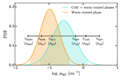
Figure 2: Log-normal probability distribution functions (PDFs) for the diffuse gas in the Milky Way (Berkhuijsen & Fletcher, 2008). The shaded contours represent the 2$\sigma$ regions for each PDF. The six $n_{\rm{amb}}$ values used in this work ($0.024,0.06,0.12,0.60,1.20,3.01\,\rm{cm^{-3}}$) are depicted along a black, horizontal line.

We study the time evolution of these SN Ia models with a self-consistent treatment of the nonequilibrium ionization (NEI) conditions in young SNRs performed by the cosmic ray-hydro-NEI code, hereafter ChN (Ellison et al., 2007; Patnaude et al., 2009; Ellison et al., 2010; Patnaude et al., 2010; Castro et al., 2012; Lee et al., 2012, 2014, 2015). ChN is a one-dimensional Lagrangian hydrodynamics code based on the multidimensional code VH-1 (e.g., Blondin & Lufkin, 1993). ChN simultaneously calculates the thermal and nonthermal emission at the FS and RS in the expanding SNR models. It couples hydrodynamics, NEI calculations, plasma emissivities, time-dependent photoionization, radiative cooling, forbidden-line emission, and diffusive shock acceleration, though we do not include diffusive shock acceleration in our calculations. ChN is a tested, flexible code that has successfully been used to model SNRs in several settings (e.g. Slane et al., 2014; Patnaude et al., 2015).

Young Ia SNRs are in NEI because, at the low densities involved ($n\,{\sim}\,1\,\rm{cm}^{-3}$), not enough time has elapsed since the ejecta were shocked to equilibrate the ionization and recombination rates (Itoh, 1977; Badenes, 2010). Consequently, these NEI plasmas are underionized when compared to collisional ionization equilibrium plasmas (Vink, 2012). The shock formation and initial plasma heating do not stem from Coulomb interactions, but from fluctuating electric and magnetic fields in these so-called collisionless shocks (Vink, 2012). In the ISM, the mean free path and the typical ages for particle-to-particle interactions are larger than those of SNRs ($\approx 10^{2}-10^{3}\,\rm{years},\approx 1-10\,\rm{pc}$).

The efficiency of electron heating at the shock transition, i.e., the value of $\beta=T_{e}/T_{i}$ at the shock, is not well determined (see, e.g., Borkowski et al., 2001). In principle, the value of $\beta$ can range between $\beta=\beta_{\rm{min}}=m_{e}/m_{i}$ and full equilibration ($\beta=1$), with partial equilibration being the most likely situation ($\beta_{\rm{min}}<\beta<1$, Borkowski et al., 2001; Ghavamian et al., 2007; Yamaguchi et al., 2014b). Here we set $\beta=\beta_{\rm{min}}$ for illustration purposes, even though previous studies (e.g., Badenes et al., 2005, 2006; Yamaguchi et al., 2014a) have shown that $\beta$ has an important effect on the Fe K$\alpha$ luminosities. This can be critical when trying to fit an SNR spectrum with a specific model, but here we are just interested in the bulk properties of the models, and we defer detailed fits to future work.

We consider uniform ambient media composed of hydrogen ($\rho_{\rm{amb}}=m_{H}\,n_{\rm{amb}}$, e.g. Badenes et al., 2003, 2006, 2008b; Patnaude & Badenes, 2017) with a range of densities: $\rho_{\rm{amb}}\,[10^{-24}\,\rm{g\,cm^{-3}}]=0.04,0.1,0.2,1.0,2.0,5.0\equiv$ $n_{\rm{amb}}\,[\rm{cm^{-3}}]=0.024,0.06,0.12,0.60,1.20,3.01$. We label each SNR model from the SN model and ambient medium density, e.g. SCH115_0p04, SCH115_0p1, SCH115_0p2, SCH115_1p0, SCH115_2p0, and SCH115_5p0. We have chosen these ambient densities to be in the same range considered by Patnaude et al. (2015). The three highest densities were used in the studies by Patnaude et al. (2012) and Yamaguchi et al. (2014a), so we will be able to compare our results to theirs. This makes a total of 48 SNR models that we evolve up to an expansion age of 5000 years. For each SNR model, we record a total of 30 time epochs, starting at 105 years. The time bins are linearly spaced at young ages and smoothly become logarithmically spaced at late ages. We also record 30 Lagrangian profiles in linearly spaced time bins for each model.

Our choice of ambient medium densities is motivated by observations of the ISM in the Milky Way. Interstellar gas can be found in five different phases (Ferrière, 1998, 2001): molecular ($T_{mol}\,{\sim}\ 10-20\ \rm{K}$, $n_{mol}\ {\sim}\ 10^{2}-10^{6}\ \rm{cm}^{-3}$), cold neutral ($T_{cold}\,{\sim}\ 50-100\ \rm{K}$, $n_{cold}\ {\sim}\ 20-50\ \rm{cm}^{-3}$), warm neutral ($T_{warm,n}\,{\sim}\ 6000-10000\ \rm{K}$, $n_{warm,n}\ {\sim}\ 0.2-0.5\ \rm{cm}^{-3}$), warm ionized ($T_{warm,i}\,{\sim}\ 8000\ \rm{K}$, $n_{warm,i}\ {\sim}\ 0.2-0.5\ \rm{cm}^{-3}$), and hot ionized ($T_{hot}\,{\sim}\ 10^{6}\ \rm{K}$, $n_{hot}\ {\sim}\ 0.0065\ \rm{cm}^{-3}$). Among these, the warm ionized phase has the highest filling factor and therefore is the most likely environment for Type Ia SNRs. Wolfire et al. (2003) gives a mean value for the neutral hydrogen density in the Galactic disk $\left<n_{HI}\right>\,=0.57\ \rm{cm}^{-3}$. More recently, Berkhuijsen & Fletcher (2008) fit log-normal distributions to the diffuse gas in the MW centered on $\left<n_{HI}\right>\,\approx 0.3\ \rm{cm}^{-3}$ (cold and warm ionized) and $\left<n_{HI}\right>\,\approx 0.1\ \rm{cm}^{-3}$ (warm ionized). We compare these distributions to our uniform density values in Figure 2.

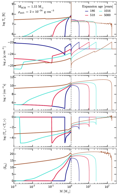
Figure 3: Time evolution of the electron temperature $T_{e}$, density $\rho$, ionization timescale $\tau=n_{e}t$, average efficiency of post-shock equilibration $T_{e}/\left<T_{i}\right>$ and average iron effective charge state $\left<z_{\rm{Fe}}\right>$ profiles as a function of the enclosed mass for model SCH115_2p0. The CD between the ejecta (thick lines) and the ambient medium swept up by the FS (thin lines) is depicted as a dashed, black vertical line, located at $1.15\,M_{\odot}$. The spatial location of the RS can be appreciated in the navy ($\sim 0.55\,M_{\odot}$), the crimson ($\sim 0.1\,M_{\odot}$) and the turquoise ($\sim 0.002\,M_{\odot}$) profiles.

Figure 3 shows the profile time evolution for a fiducial model, explosion progenitor SCH115 with an ambient density $\rho_{\rm{amb}}\,=\,2\times 10^{-24}\,\rm{g\,cm^{-3}}$. The profiles for 186 (navy), 518 (crimson), and 1016 (turquoise) years show the RS propagation toward the center of the SNR. After reaching the center, the RS bounces back and moves outwards into the previously shocked ejecta, creating more reflected shocks when it reaches the contact discontinuity (CD). This effect can be seen in the first and the second panel of Figure 3 ($T_{e}$ versus $M$, $\rho$ versus $M$) around $M\,{\sim}\,0.05\,M_{\odot}$ and $M\,{\sim}\,20\,M_{\odot}$ at 5000 years (brown).

$T_{e}$ increases with time in the inner layers after they are swept by the RS. As the SNR expands, the density $\rho$ of the shocked ejecta and ISM decreases steadily, and therefore the electron density $n_{e}$ diminishes with time. In ChN, the unshocked plasma is assumed to be 10% singly ionized.

The salient features in the evolution of this particular SNR model are representative of the entire grid. The ejecta with the highest ionization state are always found close to the contact discontinuity (CD), since they were shocked at an earlier age and higher density. Because this is also the densest region at all times, it has the highest emission measure and thus will dominate the spatially integrated X-ray emission. However, since the chemical composition of SN Ia ejecta is markedly stratified, it is often the case that different chemical elements sample different parts of the SNR structure, and therefore show different ionization timescales and electron temperatures (see the discussions in Badenes et al., 2003, 2005). This feature of the models is in good agreement with observations of young SNRs (e.g. Badenes et al., 2007).

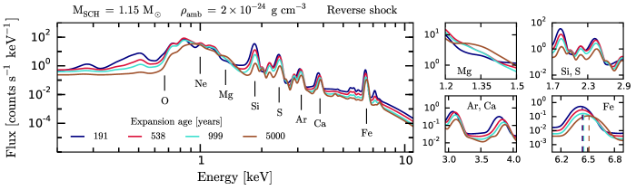
Figure 4: Integrated RS synthetic spectra normalized to $D=10$ kpc for the model shown in Figure 3 at the nearest time snapshots (see the explanation in the text). The relevant atomic transitions are labeled. The zoomed boxes depict different energy regions: Mg (up left), Si, S (up right), Ar, Ca (low left), and Fe (low right). The latter shows the time evolution of the Fe K$\alpha$ centroid energy (dashed, vertical lines).

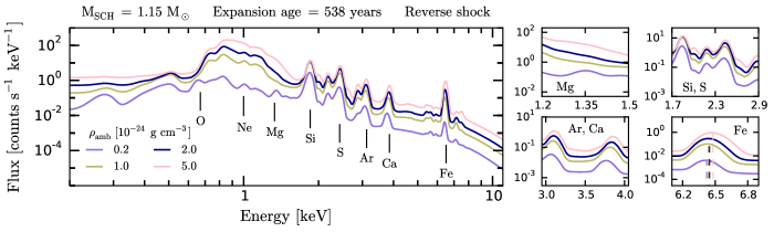
Figure 5: Integrated RS synthetic spectra normalized to $D=10$ kpc for model SCH115, for the four highest ambient densities ($\rho_{0p2}$, $\rho_{1p0}$, $\rho_{2p0}$, $\rho_{5p0}$) and a fixed expansion age of 538 years. The zoomed boxes are identical to those of Figure 4.

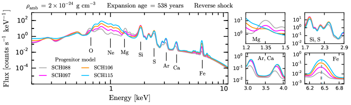
Figure 6: Integrated RS synthetic spectra normalized to $D=10$ kpc for models SCH088, SCH097, SCH106, and SCH115 at a fixed expansion age of 538 years and a fixed ambient density $\rho_{\rm{amb}}\,=\,2\times 10^{-24}\,\rm{g\,cm^{-3}}$. The zoomed boxes are identical to those of Figure 4.

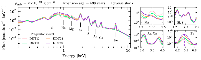
Figure 7: Integrated RS synthetic spectra normalized to $D=10$ kpc for models DDT12, DDT16, DDT24, and DDT40 at a fixed expansion age of 538 years and a fixed ambient density $\rho_{\rm{amb}}\,=\,2\times 10^{-24}\,\rm{g\,cm^{-3}}$. The zoomed boxes are identical to those of Figure 4.

2.3 Synthetic spectra

Our ejecta models determine the masses, chemical abundances, and initial velocities for each mass layer. We consider 19 elements: H, He, C, N, O, Ne, Na, Mg, Al, Si, P, S, Ar, Ca, Ti, Cr, Mn, Fe, and Ni, with a total of 297 ions. For each ion species $I$ corresponding to an element $X$, we calculate the differential emission measure (DEM) in 51 equally log-spaced $T_{e}$ bins between $10^{4}$ and $10^{9}$ K, normalized to a distance of $D=10$ kpc (Badenes et al., 2003, 2006):

$$(\rm{DEM})_{I,X}=n_{I}\,n_{e}\times\dfrac{dV}{dT_{e}}\times\dfrac{1}{4\pi D[cm]^{2}}\times\dfrac{10^{-14}}{\rm{angr}(X)}$$ (1)

where $n_{I},n_{e}$ are the ion and electron densities, $dV$ is the volume element for each layer, $\rm{angr}(X)$ are the XSPEC (Arnaud, 1996) default conversion factors for the solar abundances (Anders & Grevesse, 1989) and $10^{-14}$ is a normalization applied to the emissivities in XSPEC. We couple these DEMs to the atomic emissivity code PyAtomDB (AtomDB version 3.0.9; see, e.g., Foster et al., 2012, 2014) in order to calculate the emitted flux for each model at a given photon energy. We separate the RS and the FS contribution and generate nonconvolved photon spectra in 10000 equally spaced bins of size 1.2 eV between 0.095 and 12.094 keV. Thermal broadening and line splitting due to bulk motions are ignored in this version of the synthetic spectra, but we plan to include them in future versions.

Table 2: Data corresponding to the Ia SNRs in our sample.

Name	$E_{\,\rm{Fe}_{K\alpha}}$	$F_{\,\rm{Fe}_{K\alpha}}$1	Distance	$L_{\,\rm{Fe}_{K\alpha}}$	Radius	Age	References
	$\mathrm{eV}$	($\mathrm{10^{-5}\,ph\,cm^{-2}\,s^{-1}}$)	($\mathrm{kpc}$)	($\mathrm{10^{40}\,ph\,s^{-1}}$)	($\mathrm{pc}$)	($\mathrm{years}$)
Kepler	$6438\pm 1$	$34.6\pm 0.2$	$3.0-6.4$	$91\pm 66$	$2.3\pm 0.9$	$414$	1, 2, 3, 4
3C 397	$6556^{+4}_{-3}$	$13.7\pm 0.4$	$6.5-9.5$	$105\pm 39$	$5.3\pm 0.5$	$1350-5300$	5, 6
Tycho	$6431\pm 1$	$61.0\pm 0.4$	$2.5-3.0$	$55\pm 10$	$3.3\pm 0.3$	$446$	7, 8
RCW 86	$6408^{+4}_{-5}$	$14.0\pm 0.7$	$2.5$	$10.5\pm 0.5$	$16$	$1833$	9, 10, 11
SN 1006	$6429\pm 10$	$2.55\pm 0.43$	$2.2$	$1.5\pm 0.3$	$10$	$1012$	12
G337.2$-$0.7	$6505^{+26}_{-31}$	$0.21\pm 0.06$	$2.0-9.3$	$0.8\pm 1.1$	$4.9\pm 3.2$	$5000-7000$	13
G344.7$-$0.1	$6463^{+9}_{-10}$	$4.03\pm 0.33$	$14$	$95\pm 8$	$16$	$3000-6000$	14
G352.7$-$0.1	$6443^{+8}_{-12}$	$0.82\pm 0.08$	$7.5$	$5.5\pm 0.5$	$6$	${\sim}\,1600$	15, 16
N103B	$6545\pm 6$	$2.15\pm 0.10$	50	$643\pm 30$	$3.6$	${\sim}\,860$	17, 18, 19
0509$-$67.5	$6425^{+14}_{-15}$	$0.32\pm 0.04$	504	$96\pm 12$	$3.6$	${\sim}\,400$	18, 20, 21
0519$-$69.0	$6498^{+6}_{-8}$	$0.93\pm 0.05$	504	$278\pm 15$	$4.0$	${\sim}\,600$	18, 21, 22
G1.9+0.3	$6444$	-	${\sim}\,8.5$	1	${\sim}\,2.0$	${\sim}150$	23, 24
DEM L71	$6494\pm 58$	-	504	$26^{+8}_{-9}$	8.6	${\sim}\,4700$	25, 26, 27

We generate synthetic spectra for both RS and FS convolved with the Suzaku spectral and ancillary responses (Mitsuda et al., 2007). We choose Suzaku over Chandra or XMM–Newton for illustration purposes, given its superior spectral resolution around the K$\alpha$ transitions from Fe-peak elements ($\approx 5.5-8.0$ keV). For simplicity, we do not include the effect of interstellar absorption (relevant below $\sim$ 1 keV). In any case, most Ia SNRs have column densities smaller than $10^{22}\,\rm{cm^{-2}}$ (e.g., Lewis et al., 2003; Warren & Hughes, 2004; Badenes et al., 2006; Reynolds et al., 2007; Kosenko et al., 2010; Yamaguchi et al., 2014b). All the convolved and nonconvolved spectra are publicly available in a repository (https://github.com/hector-mr).

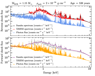
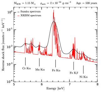
Figure 8: Left: Photon, Suzaku and XRISM spectra for model SCH115_2p0 at a fixed expansion age of 538 years (Top: Reverse shock. Bottom: Forward shock). Right: Zoomed-in reverse shock spectra around the Fe K$\alpha$ complex. The relevant atomic transitions are labeled.

Figure 4 shows the time evolution of the X-ray flux from the RS for the fiducial model shown in Figure 3. We do not show the thermal spectrum from the FS because it is very weak or absent in many young Type Ia SNRs, often being replaced by nonthermal synchrotron emission (e.g., Warren & Hughes, 2004; Warren et al., 2005; Cassam-Chenaï et al., 2008). While the ChN code has the capability to model the modification of the FS dynamics and spectrum due to particle acceleration processes (e.g., Slane et al., 2014), this falls outside the scope of the present work. The thermal RS flux shown in Figure 4 decreases with time because the ejecta density decreases steadily, and the emission measure scales as $n_{e}^{\,2}$. This effect usually dominates over the steady increase in $T_{e}$ due to electron-ion collisions in the shocked plasma (see Figure 3), which tends to increase the emitted flux. The centroids of the K$\alpha$ transitions move to higher energies with time, especially for Ca, Fe, and Ni, because those elements have a large range of charge states. For elements with lower atomic numbers, like Si and S, the centroid energies saturate when the He-like ions become dominant, and then the Ly$\alpha$ transitions from H-like ions begin to appear. For this fiducial model, the spectrum at 5000 years (brown) shows a Ti K$\alpha$ feature at $\approx 4.5$ keV.

Figure 5 shows the effect of varying the ambient medium density on the RS spectra for the same explosion model (SCH115) at a fixed expansion age of 538 years. Higher $\rho_{\rm{amb}}$ translate into higher ejecta densities due to a slower ejecta expansion. This yields higher fluxes and centroid energies for all transitions due to the increased rate of ionizing collisions. As $\rho_{\rm{amb}}$ increases, the Fe L-shell transitions dominate the flux around ${\sim}\,$1 keV. Figures 6 and 7 show the RS spectra for all sub-M_Ch and M_Ch progenitor models with the same $\rho_{\rm{amb}}\,\left(2\times 10^{-24}\,\rm{g\,cm^{-3}}\right)$ and expansion age (538 years). The differences between the models are largest in the bands dominated by the Fe L-shell and K-shell transitions. This is due to the different distribution of Fe-peak elements in the inner ejecta region for different models. In sub-M_Ch models with larger masses and M_Ch models with higher DDT transition densities, the Fe-peak elements extend further out in Lagrangian mass coordinate (see Figure 1). This translates into very different shocked masses of each element at a given age and ambient medium density for different explosion models, and therefore into large differences in the X-ray spectra. For Si and S, on the other hand, most of the ejected mass is already shocked at 538 years in all models ($M_{\rm{shocked}}=0.81,0.90,0.98,1.06\,M_{\odot}$ for models SCH088_2p0, SCH097_2p0, SCH106_2p0, SCH115_2p0, and $M_{\rm{shocked}}=1.16,1.18,1.20,1.21\,M_{\odot}$ for models DDT12_2p0, DDT16_2p0, DDT24_2p0, DDT40_2p0, shown in Figure 1), which translates into a smaller dynamic range of X-ray emitting masses and therefore smaller differences for the corresponding lines in the spectra. Elements like Mg and O are also fully shocked at this age, but their spectral blends show larger variations than those of Si and S because the dynamic range in ejected masses is much larger (see Table 1).

Our spectral models can also be convolved with the response matrices for future facilities, like the X-Ray Imaging and Spectroscopy Mission (XRISM, a.k.a. X-Ray Astronomy Recovery Mission, XARM, Tashiro et al., 2018) or Athena (Nandra et al., 2013). The left panel of Figure 8 shows the RS and FS spectra for model SCH115_2p0 at 538 years, unconvolved (photon flux) and after convolution with both Suzaku and XRISM responses. It is worth noting that XRISM will not be able to separate the FS and RS for the remnants in our sample. The improved energy resolution of XRISM reveals a wealth of transitions that cannot be seen with Suzaku, as shown in the right panel of Figure 8. There are two transitions at $\approx$ 5.4 and $\approx$ 5.65 keV in both the Suzaku and the XRISM synthetic spectrum that do not appear in real Suzaku observations. We defer this to a future study.

The one-dimensional nature of our models deserves some comments. Multidimensional hydrodynamics coupled with NEI calculations (Warren & Blondin, 2013; Orlando et al., 2016) are computationally expensive, and do not allow to produce extensive model grids for an exhaustive exploration of parameter space like the one we present here. The results from Warren & Blondin (2013), who studied the impact of clumping and Rayleigh-Taylor instabilities in the morphology and ionization (but not emitted spectra) of Type Ia SNRs in 3D, do not show major deviations from one-dimensional calculations.

3 Discussion

3.1 Type Ia SNRs: Bulk properties

Here we describe the bulk properties (expansion age, radius, Fe K$\alpha$ centroid, and Fe K$\alpha$ luminosity) of our M_Ch and sub-M_Ch models and compare them with the available observational data for Ia SNRs. We use the Fe K$\alpha$ blend because it is sensitive to the electron temperature and ionization timescale in SNRs, with the centroid energy being a strong function of mean charge state (Vink, 2012; Yamaguchi et al., 2014a, b). This results in a clear division between Ia SNRs, which tend to interact with a low-density ambient medium, and core collapse (CC) SNRs, which often evolve in the high density CSM left behind by their massive and short-lived progenitors (first noted by Yamaguchi et al. 2014b, see also Patnaude et al. 2015; Patnaude & Badenes 2017). In their analysis, Yamaguchi et al. (2014a) already found that the bulk properties of the SNRs identified as Ia in their sample (those with Fe K$\alpha$ centroid energies below 6.55 keV) were well reproduced by the M_Ch  uniform ambient medium models of Badenes et al. (2003, 2005). Here, we perform a more detailed comparison to our models, which also assume a uniform ambient medium, but are based on an updated code and atomic data, and include both M_Ch and sub-M_Ch progenitors. We also comment briefly on some individual objects of interest.

We calculate the Fe K$\alpha$ centroid energy $E_{\,\rm{Fe}_{K\alpha}}$ and luminosity $L_{\,\rm{Fe}_{K\alpha}}$ for each model as

$$E_{\,\rm{Fe}_{K\alpha}}=\dfrac{{\int_{E_{\rm{min}}}^{E_{\rm{max}}}\left(F\times\,E\right)\,dE}}{{\int_{E_{\rm{min}}}^{E_{\rm{max}}}F\,dE}}=\dfrac{{\sum_{i\subseteq}}\,F_{i}\times E_{i}\times dE_{i}}{{\sum_{i\subseteq}}\,F_{i}\times dE_{i}}$$ (2)

$$F_{\,\rm{Fe}_{K\alpha}}={\int_{E_{\rm{min}}}^{E_{\rm{max}}}}F\,dE={\sum_{i\subseteq}}\,F_{i}\times dE_{i}$$ (3)

$$L_{\,\rm{Fe}_{K\alpha}}=4\pi D[\textrm{cm}]^{2}\times\,F_{\,\rm{Fe}_{K\alpha}}$$ (4)

where $F$ is the differential flux from the nonconvolved spectrum after continuum subtraction, $dE$ is the constant (1.2 eV) energy step, and $E_{\rm{min}}-E_{\rm{max}}$ is an energy interval that covers the entire Fe K$\alpha$ complex (6.3 $-$ 6.9 keV). We only compute these numbers when the Fe K$\alpha$ emission is clearly above the continuum.

Table 2 summarizes the relevant observational properties of the 13 Type Ia SNRs in our sample. The data are taken from Yamaguchi et al. (2014a) (Suzaku observations). We also include the Chandra measurements for G1.9+0.3 (Borkowski et al., 2013) and the XMM–Newton results for DEM L71 (Maggi et al., 2016). The contours in Figures 9$-$12 show the parameter space spanned by our models, with symbols indicating the observed properties of individual SNRs. We display $L_{\,\rm{Fe}_{K\alpha}}$ versus $E_{\,\rm{Fe}_{K\alpha}}$ (Figure 9), $E_{\,\rm{Fe}_{K\alpha}}$ versus FS radius ($R_{\rm{FS}}$, Figure 10), $E_{\,\rm{Fe}_{K\alpha}}$ versus expansion age (Figure 11), and $R_{\rm{FS}}$ versus expansion age (Figure 12).

The main features of the models shown in these plots merit some comments. In Figures 9$-$11, for the models with $\rho_{1p0}$, $\rho_{2p0}$ and $\rho_{5p0}$, $E_{\,\rm{Fe}_{K\alpha}}$ decreases for a short time $\approx 1000-2000$ years after the explosion instead of increasing monotonically with time. This is due to the reheating of the shocked ejecta after the RS bounces at the SNR center. The reshocked material becomes denser and hotter, and therefore more luminous. This results in a lower luminosity-weighted ionization state for the shocked ejecta, which prior to RS bounce was dominated by the dense, highly ionized material close to the CD. As time goes on and the entire ejecta is reshocked, the material close to the CD dominates the spectrum again, and the ionization state continues to increase monotonically. The strength of this feature is due to the spherical symmetry of our models, at least to some extent, but we expect a qualitatively similar (if weaker) effect in reality. We note that, although our model predictions are qualitatively similar to those from Badenes et al. (2003, 2005, 2006), Yamaguchi et al. (2014a) and Patnaude et al. (2015), there are small deviations $-$ for instance, we predict a slightly higher $E_{\,\rm{Fe}_{K\alpha}}$ for the same ambient medium density and age (${\sim}$ 6.6 keV versus ${\sim}$ 6.5 keV). This is likely due to differences in the hydrodynamic code, atomic data, and explosion models. In addition, Patnaude et al. (2015) stopped their calculations when the RS first reached the center of the SNR, while we continue ours until the models reach an age of 5000 years.

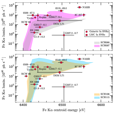
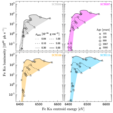
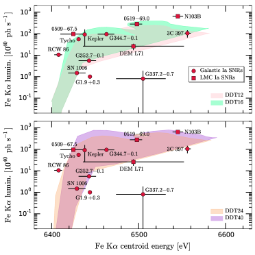
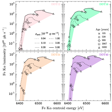
Figure 9: Left: Centroid energies and line luminosities of Fe K$\alpha$ emission from various Type Ia SNRs in our Galaxy (circles) and the LMC (squares). The shaded regions depict the Fe K$\alpha$ centroids and luminosities predicted by our theoretical sub-M_Ch and M_Ch models with various uniform ISM densities (SCH088: gray; SCH097: magenta; SCH106: orange; SCH115: blue; DDT12: pink; DDT16: green; DDT24: light brown; DDT40: purple). Right: Individual tracks for each model. The $L_{\,\rm{Fe}_{K\alpha}}$ $-$ $E_{\,\rm{Fe}_{K\alpha}}$ tracks corresponding to the two lowest ambient densities ($\rho_{0p04}$, $\rho_{0p1}$) do not appear in the plots because their $L_{\,\rm{Fe}_{K\alpha}}$ values are considerably small.

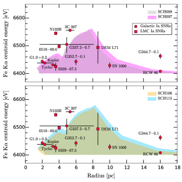
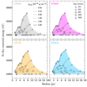
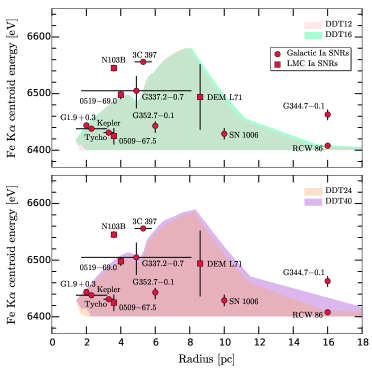
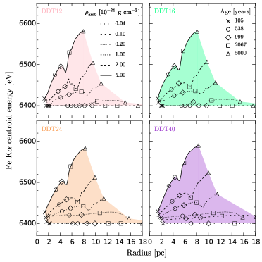
Figure 10: Fe K$\alpha$ centroid energy versus forward shock radius for the Type Ia SNRs in our sample. The shaded regions correspond to the models shown in Figure 9.

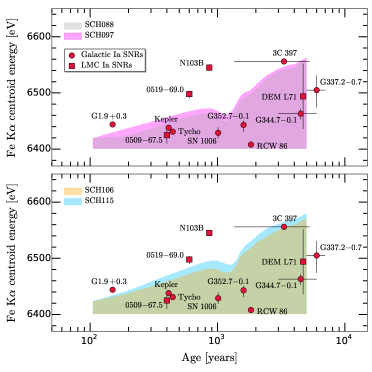
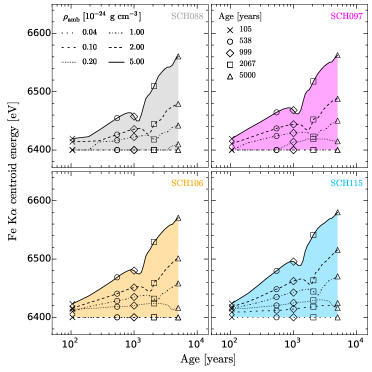
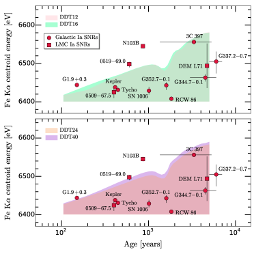
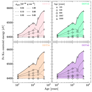
Figure 11: Fe K$\alpha$ centroid energy versus expansion age for the Type Ia SNRs in our sample. The shaded regions correspond to the models shown in Figures 9 and 10.

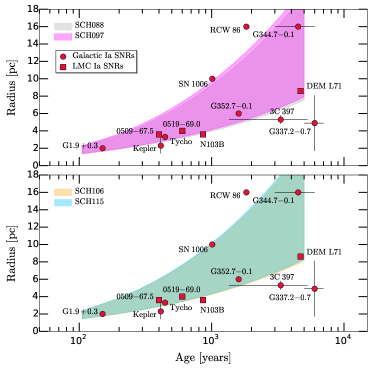
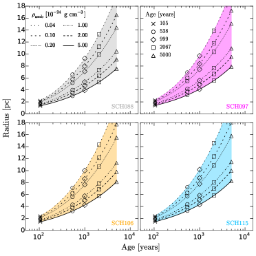
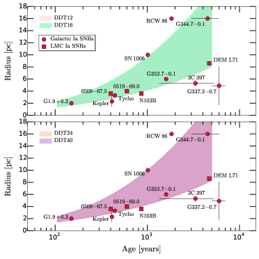
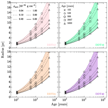
Figure 12: Forward shock radius versus expansion age for the Type Ia SNRs in our sample. The shaded regions correspond to the models shown in Figures 9, 10 and 11.

Figures 9$-$12 show that the parameter space covered by our spherically symmetric, uniform ambient medium models is in good agreement with the observed data. While there are exceptions, which we discuss in detail below, it is clear that our models are a good first approximation to interpret the bulk dynamics of real Type Ia SNRs, and can be used to infer their fundamental physical properties. For example, denser ambient media and more energetic progenitor models predict higher $E_{\,\rm{Fe}_{K\alpha}}$ and $L_{\,\rm{Fe}_{K\alpha}}$ at a given expansion age, as seen in Figure 9. Thus, the SNRs with the highest $L_{\,\rm{Fe}_{K\alpha}}$, like 0519$-$69.0 and 0509$-$67.5, are only compatible with the brightest, most Fe-rich progenitor models (SCH106, SCH115, DDT16, and DDT24). The Fe K$\alpha$ emission from SNR N103B, in particular, can only be reproduced by model DDT40 at the highest ambient medium density. As shown in Figures 10 and 12, $R_{\rm{FS}}$ has a weak dependence on the ejecta mass, but it is quite sensitive to the ambient density because $R_{\rm{FS}}\propto M^{1/3}\rho^{-1/3}$ (McKee & Truelove, 1995). Therefore, objects surrounded by low-density media (e.g. RCW 86, SN 1006, and G344.7$-$0.1) clearly stand apart from those evolving in high density media (e.g. 3C 397, N103B, and Kepler): the former have large $R_{\rm{FS}}$ and low $E_{\,\rm{Fe}_{K\alpha}}$ centroids, while the latter have small $R_{\rm{FS}}$ and high $E_{\,\rm{Fe}_{K\alpha}}$. We note that the ages of these remnants differ from one another. In general, the densities we infer from simple comparisons to our models are in good agreement with detailed studies of individual objects. For instance, Someya et al. (2014) and Williams et al. (2014) determined $n_{\rm{amb}}\gtrsim 2.0\,\rm{cm^{-3}}$ for N103B, and Leahy & Ranasinghe (2016) found $n_{\rm{amb}}\ {\sim}\ 2-5\,\rm{cm}^{-3}$ for 3C 397, which are close to the highest value of $\rho_{\rm{amb}}$ in our grid ($n_{\rm{amb}}=3.01\,\rm{cm^{-3}}$).

For all the observables shown in Figures 9$-$12, the main sources of variation in the models are the ambient density and the expansion age. This implies that the details of the energetics and chemical composition in the supernova model, and in particular whether the progenitor was M_Ch or sub-M_Ch, are not the main drivers for the bulk dynamics of Type Ia SNRs. This does not imply that our SNR models do not have the power to discriminate Type Ia SN explosion properties - detailed fits to the X-ray spectra of individual objects have shown that they can do this very well (e.g., Badenes et al., 2006, 2008a; Patnaude et al., 2012). However, the bulk SNR properties on their own are not very sensitive to the explosion properties, especially for objects whose expansion ages or distances are not well determined. To discriminate explosion properties, additional information needs to be taken into account, like specific line flux ratios (e.g. $\rm{Si\,\,K\alpha\,/\,Fe\,\,K\alpha}$, $\rm{S\,\,K\alpha\,/\,Fe\,\,K\alpha}$, and $\rm{Ar\,\,K\alpha\,/\,Fe\,\,K\alpha}$), which can distinguish M_Ch from sub-M_Ch progenitors, or even better, detailed fits to the entire X-ray spectrum, which can reveal a wealth of information about the explosion (e.g., Badenes et al., 2006, 2008a; Patnaude et al., 2012). We defer these applications of our models to future work.

To evaluate the degree to which a particular model works well for a given SNR, it is important to examine all its bulk properties at the same time. By doing this, we can single out individual objects whose bulk dynamics cannot be reproduced by our models, modulo any uncertainties in the expansion age and distance. Not surprisingly, the SNR that shows the largest deviation from our models is RCW 86. This remnant is known to be expanding into a low-density cavity, presumably excavated by a fast, sustained outflow from the SN progenitor (Badenes et al., 2007; Williams et al., 2011; Broersen et al., 2014), and therefore its $R_{\rm{FS}}$ is too large for its expansion age and $E_{\,\rm{Fe}_{K\alpha}}$. In addition, its classification as a Type Ia SNR is still under debate (Gvaramadze et al., 2017). The Galactic SNR G344.7$-$0.1 also shows a similar deviation, albeit less strong, but this might be related to an overestimated distance and $R_{\rm{FS}}$ (Yamaguchi et al., 2012b, and references therein).

Among the objects interacting with low-density media, the size of SN 1006 is compatible with our lowest-density models, which agrees with the value $n_{\rm{amb}}\ {\sim}\ 0.03\,\rm{cm}^{-3}$ found by Yamaguchi et al. (2008), and its $E_{\,\rm{Fe}_{K\alpha}}$ and $L_{\,\rm{Fe}_{K\alpha}}$ are within the parameter space covered by the models. We examine the case of SN 1006 in more detail in Section 3.2. Among the objects interacting with high density media, 3C 397 and N103B have $E_{\,\rm{Fe}_{K\alpha}}$ values that are too high for their physical sizes and expansion ages. This has been pointed out by Patnaude & Badenes (2017), and could be due to some sort of interaction with dense material, possibly (but not necessarily) a CSM modified by the SN progenitor (Safi-Harb et al., 2005; Williams et al., 2014; Li et al., 2017). Remarkably, the bulk dynamics of the Kepler SNR, which is often invoked as an example of CSM interaction in Type Ia SNRs (e.g., Reynolds et al., 2007; Chiotellis et al., 2012; Burkey et al., 2013) are compatible with a uniform ambient medium interaction, although a detailed spectral analysis suggests the presence of a small cavity around its progenitor system (Patnaude et al., 2012). Finally, the Galactic SNR G337.2$-$0.7 appears to be underluminous for its relatively high $E_{\,\rm{Fe}_{K\alpha}}$, but this could be due to the large uncertainty in its distance (Rakowski et al., 2006).

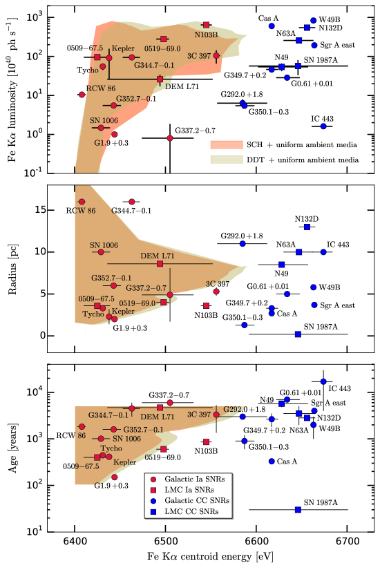
Figure 13: Fe K$\alpha$ luminosity, radius and expansion age as a function of the Fe K$\alpha$ centroid energy for Ia (red) and CC (blue) SNRs (Lovchinsky et al., 2011; Vogt & Dopita, 2011; Park et al., 2012; Tian & Leahy, 2014; Yamaguchi et al., 2014a, and references therein). For a more updated sample and further discussion, see Maggi & Acero (2017). The shaded regions depict the predictions from our theoretical M_Ch (khaki) and sub-M_Ch (dark orange) models with uniform ISM densities.

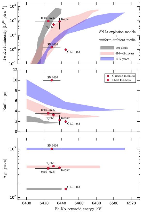
Figure 14: Fe K$\alpha$ luminosity, radius and expansion age as a function of the Fe K$\alpha$ centroid energy for G1.9+0.3, 0509$-$67.5, Kepler, Tycho, and SN 1006. The shaded regions depict the predictions from our theoretical M_Ch and sub-M_Ch models with uniform ISM densities for different expansion ages: 150 (black), 416$-$444 (light coral), and 1012 (blue) years.

We summarize our comparisons between models and data in Figure 13, which shows $L_{\,\rm{Fe}_{K\alpha}}$, $R_{\rm{FS}}$ and expansion age for our M_Ch and sub-M_Ch models and for the SNRs as a function of $E_{\,\rm{Fe}_{K\alpha}}$, the only property that can be determined from the observations alone. We re-emphasize that our uniform ambient medium, spherically symmetric models, can reproduce the bulk dynamics of most Type Ia SNRs quite well. This suggests that, unlike CC SN progenitors, most Type Ia SN progenitors do not strongly modify their circumstellar environments, as previously noted by Badenes et al. (2007), Yamaguchi et al. (2014a), Patnaude & Badenes (2017), and other authors. This conclusion is in good agreement with the (hitherto unsuccessful) attempts to detect prompt X-ray and radio emission from extragalactic Type Ia SNe (Margutti et al., 2014; Chomiuk et al., 2016), but we note that SNR studies probe spatial and temporal scales (${\sim}$ pc and ${\sim}\,10^{5}$ years, Patnaude & Badenes, 2017) that are more relevant for the pre-SN evolution of Type Ia progenitor models. In this sense, the lack of a strongly modified CSM sets Type Ia SNRs clearly apart from CC SNRs (Yamaguchi et al., 2014a), which we also include in Figure 13 for comparison. The only two SNRs with well-determined properties that are clearly incompatible with our uniform ambient medium models are RCW 86 and N103B. These SNRs are probably expanding into some sort of modified CSM. In the case of RCW 86, the modification is very strong, and clearly due to the formation of a large cavity by the progenitor. In the case of N103B (and perhaps also 3C 397), the modification could be due to some dense material left behind by the progenitor, but detailed models with nonuniform ambient media are required to verify or rule out this claim. In any case, it is clear from Figure 13 that the modification of the CSM by the progenitor in N103B must be much weaker than what is seen around typical CC SNRs.

3.2 Type Ia SNRs: Remnants with well-determined expansion ages

A reduced subset of Type Ia SNRs have well-determined ages, either because they are associated with historical SNe (Kepler, Tycho, and SN 1006 have ages of 414, 446, and 1012 years, respectively), because they have well-observed light echoes (0509$-$67.5 has an age of ${\sim}\,$ 400 years, Rest et al., 2008), or because their dynamics put very strong constraints on their age (G1.9+0.3 has an age of ${\sim}\,$ 150 years, Reynolds et al., 2008; Carlton et al., 2011; De Horta et al., 2014; Sarbadhicary et al., 2017). These objects are particularly valuable benchmarks for our models, because their known ages remove an important source of uncertainty in the interpretation of their bulk dynamics.

We perform more detailed comparisons for this set of objects by taking our models at 150 years (G1.9+0.3), 416$-$444 years (0509$-$67.5, Kepler, and Tycho) and 1012 years (SN 1006). Figure 14 shows the same quantities as Figure 13, but here we display the parameter space covered by our M_Ch and sub-M_Ch models at all densities for each of the three age ranges mentioned above. The models at 416$-$444 years can reproduce the observed properties of Kepler, Tycho, and 0509$-$67.5 quite well, even with the added constraints from the known expansion ages, but we stress that detailed fits to the entire X-ray spectra might reveal additional information (see Patnaude et al. 2012 for Kepler, Slane et al. 2014 for Tycho). In any case, we can say that the bulk dynamics of these three objects disfavor variations from a uniform medium interaction as large as those seen in typical CC SNRs. We note that we have made no attempt to quantify the extent of the deviation from a uniform ambient medium that could be accommodated while still yielding results that are consistent with the observations, as it is beyond the scope of the present work.

For SN 1006, $R_{\rm{FS}}$, $E_{\,\rm{Fe}_{K\alpha}}$, and $L_{\,\rm{Fe}_{K\alpha}}$ are well reproduced by our models at 1012 years; though, given its surrounding ambient density and physical size, $E_{\,\rm{Fe}_{K\alpha}}$ is larger than can be explained by a uniform ambient medium interaction. For G1.9+0.3, $R_{\rm{FS}}$ and $L_{\,\rm{Fe}_{K\alpha}}$ are close to the values predicted by our models at 150 years, but $E_{\,\rm{Fe}_{K\alpha}}$ is too high to be reconciled with a uniform ambient medium interaction. In both cases, the bulk properties of the SNRs might indicate an early interaction with some sort of modified CSM. For SN 1006, this might be a low-density cavity, perhaps smaller in size than the SNR. For G1.9+0.3, a thin, dense shell that changed the ionization state without strongly affecting the dynamics might have been involved, as suggested by Chakraborti et al. (2016). In both cases, a detailed exploration of the parameter space for CSM interaction in Type Ia SNRs is required to confirm or rule out specific scenarios.’

4 Conclusions

We have presented a new grid of one-dimensional models for young SNRs arising from the interaction between Type Ia explosions with different M_Ch and sub-M_Ch progenitors and a uniform ambient medium. We have generated synthetic X-ray spectra for each model at different expansion ages, separating the reverse and forward shock contributions. Our model spectra are publicly available, and can easily be convolved with the spectral responses of current and future X-ray missions like Chandra, XRISM, and Athena. We have studied the bulk spectral and dynamical properties of our models (Fe K$\alpha$ centroid energies and luminosities, radii, and expansion ages), and have found that they provide an excellent match to the observations of most known Type Ia SNRs, indicating that the majority of SN Ia progenitors do not seem to substantially modify their surroundings on scales of a few parsecs, at least in comparison with CC SN progenitors. In our models, the ambient medium density and expansion age are the main contributors to the diversity of the bulk SNR properties, but detailed fits to X-ray spectra can discriminate progenitor properties. We have also identified a few objects that cannot be easily reproduced by SNR models with a uniform ambient medium interaction, notably RCW 86, which is known to be a cavity explosion, and N103B, which is probably interacting with dense material of some sort. A detailed exploration of the parameter space for CSM interaction in Type Ia SNRs is required to gain further insight from these objects.

References

- Anders & Grevesse (1989) Anders, E., & Grevesse, N. 1989, Geochim. Cosmochim. Acta, 53, 197
- Andrews et al. (2016) Andrews, B. H., Weinberg, D. H., Schönrich, R., & Johnson, J. A. 2016, ArXiv e-prints, arXiv:1604.08613
- Arnaud (1996) Arnaud, K. A. 1996, in Astronomical Society of the Pacific Conference Series, Vol. 101, Astronomical Data Analysis Software and Systems V, ed. G. H. Jacoby & J. Barnes, 17
- Ashall et al. (2016) Ashall, C., Mazzali, P. A., Pian, E., & James, P. A. 2016, MNRAS, 463, 1891
- Asplund et al. (2009) Asplund, M., Grevesse, N., Sauval, A. J., & Scott, P. 2009, ARA&A, 47, 481
- Astropy Collaboration et al. (2013) Astropy Collaboration, Robitaille, T. P., Tollerud, E. J., et al. 2013, A&A, 558, A33
- Badenes (2010) Badenes, C. 2010, Proceedings of the National Academy of Science, 107, 7141
- Badenes et al. (2005) Badenes, C., Borkowski, K. J., & Bravo, E. 2005, ApJ, 624, 198
- Badenes et al. (2006) Badenes, C., Borkowski, K. J., Hughes, J. P., Hwang, U., & Bravo, E. 2006, ApJ, 645, 1373
- Badenes et al. (2003) Badenes, C., Bravo, E., Borkowski, K. J., & Domínguez, I. 2003, ApJ, 593, 358
- Badenes et al. (2008a) Badenes, C., Bravo, E., & Hughes, J. P. 2008a, ApJ, 680, L33
- Badenes et al. (2007) Badenes, C., Hughes, J. P., Bravo, E., & Langer, N. 2007, ApJ, 662, 472
- Badenes et al. (2008b) Badenes, C., Hughes, J. P., Cassam-Chenaï, G., & Bravo, E. 2008b, ApJ, 680, 1149
- Berkhuijsen & Fletcher (2008) Berkhuijsen, E. M., & Fletcher, A. 2008, MNRAS, 390, L19
- Betoule et al. (2014) Betoule, M., Kessler, R., Guy, J., et al. 2014, A&A, 568, A22
- Blondin & Lufkin (1993) Blondin, J. M., & Lufkin, E. A. 1993, ApJS, 88, 589
- Blondin et al. (2017) Blondin, S., Dessart, L., Hillier, D. J., & Khokhlov, A. M. 2017, MNRAS, 470, 157
- Borkowski et al. (2001) Borkowski, K. J., Lyerly, W. J., & Reynolds, S. P. 2001, ApJ, 548, 820
- Borkowski et al. (2013) Borkowski, K. J., Reynolds, S. P., Hwang, U., et al. 2013, ApJ, 771, L9
- Bravo et al. (2018) Bravo, E., Badenes, C., & Martínez-Rodríguez, H. 2018, Accepted for publication in MNRAS
- Bravo et al. (2016) Bravo, E., Gil-Pons, P., Gutiérrez, J. L., & Doherty, C. L. 2016, A&A, 589, A38
- Bravo & Martínez-Pinedo (2012) Bravo, E., & Martínez-Pinedo, G. 2012, Phys. Rev. C, 85, 055805
- Broersen et al. (2014) Broersen, S., Chiotellis, A., Vink, J., & Bamba, A. 2014, MNRAS, 441, 3040
- Burkey et al. (2013) Burkey, M. T., Reynolds, S. P., Borkowski, K. J., & Blondin, J. M. 2013, ApJ, 764, 63
- Carlton et al. (2011) Carlton, A. K., Borkowski, K. J., Reynolds, S. P., et al. 2011, ApJ, 737, L22
- Cassam-Chenaï et al. (2008) Cassam-Chenaï, G., Hughes, J. P., Reynoso, E. M., Badenes, C., & Moffett, D. 2008, ApJ, 680, 1180
- Castro et al. (2013) Castro, D., Lopez, L. A., Slane, P. O., et al. 2013, ApJ, 779, 49
- Castro et al. (2012) Castro, D., Slane, P., Ellison, D. C., & Patnaude, D. J. 2012, ApJ, 756, 88
- Chakraborti et al. (2016) Chakraborti, S., Childs, F., & Soderberg, A. 2016, ApJ, 819, 37
- Chiotellis et al. (2012) Chiotellis, A., Schure, K. M., & Vink, J. 2012, A&A, 537, A139
- Chomiuk et al. (2016) Chomiuk, L., Soderberg, A. M., Chevalier, R. A., et al. 2016, ApJ, 821, 119
- De Horta et al. (2014) De Horta, A. Y., Filipovic, M. D., Crawford, E. J., et al. 2014, Serbian Astronomical Journal, 189, 41
- Ellison et al. (2007) Ellison, D. C., Patnaude, D. J., Slane, P., Blasi, P., & Gabici, S. 2007, ApJ, 661, 879
- Ellison et al. (2010) Ellison, D. C., Patnaude, D. J., Slane, P., & Raymond, J. 2010, ApJ, 712, 287
- Ferrière (1998) Ferrière, K. 1998, ApJ, 497, 759
- Ferrière (2001) Ferrière, K. M. 2001, Reviews of Modern Physics, 73, 1031
- Foster et al. (2014) Foster, A., Smith, R. K., Yamaguchi, H., Ji, L., & Wilms, J. 2014, in American Astronomical Society Meeting Abstracts, Vol. 223, American Astronomical Society Meeting Abstracts #223, 232.03
- Foster et al. (2012) Foster, A. R., Ji, L., Smith, R. K., & Brickhouse, N. S. 2012, ApJ, 756, 128
- Ghavamian et al. (2007) Ghavamian, P., Laming, J. M., & Rakowski, C. E. 2007, ApJ, 654, L69
- Giacani et al. (2009) Giacani, E., Smith, M. J. S., Dubner, G., et al. 2009, A&A, 507, 841
- Goldstein & Kasen (2018) Goldstein, D. A., & Kasen, D. 2018, ApJ, 852, L33
- Gvaramadze et al. (2017) Gvaramadze, V. V., Langer, N., Fossati, L., et al. 2017, Nature Astronomy, 1, 0116
- Hachisu et al. (1996) Hachisu, I., Kato, M., & Nomoto, K. 1996, ApJ, 470, L97
- Han & Podsiadlowski (2004) Han, Z., & Podsiadlowski, P. 2004, MNRAS, 350, 1301
- Hughes et al. (2003) Hughes, J. P., Ghavamian, P., Rakowski, C. E., & Slane, P. O. 2003, ApJ, 582, L95
- Hunter (2007) Hunter, J. D. 2007, Computing in Science and Engineering, 9, 90
- Iben & Tutukov (1984) Iben, Jr., I., & Tutukov, A. V. 1984, ApJS, 54, 335
- Itoh (1977) Itoh, H. 1977, PASJ, 29, 813
- Khokhlov (1991) Khokhlov, A. M. 1991, A&A, 245, 114
- Kobayashi et al. (2006) Kobayashi, C., Umeda, H., Nomoto, K., Tominaga, N., & Ohkubo, T. 2006, ApJ, 653, 1145
- Kosenko et al. (2010) Kosenko, D., Helder, E. A., & Vink, J. 2010, A&A, 519, A11
- Kushnir et al. (2013) Kushnir, D., Katz, B., Dong, S., Livne, E., & Fernández, R. 2013, ApJ, 778, L37
- Leahy & Ranasinghe (2016) Leahy, D. A., & Ranasinghe, S. 2016, ApJ, 817, 74
- Lee et al. (2012) Lee, S.-H., Ellison, D. C., & Nagataki, S. 2012, ApJ, 750, 156
- Lee et al. (2014) Lee, S.-H., Patnaude, D. J., Ellison, D. C., Nagataki, S., & Slane, P. O. 2014, ApJ, 791, 97
- Lee et al. (2015) Lee, S.-H., Patnaude, D. J., Raymond, J. C., et al. 2015, ApJ, 806, 71
- Lee et al. (2013) Lee, S.-H., Slane, P. O., Ellison, D. C., Nagataki, S., & Patnaude, D. J. 2013, ApJ, 767, 20
- Lewis et al. (2003) Lewis, K. T., Burrows, D. N., Hughes, J. P., et al. 2003, ApJ, 582, 770
- Li et al. (2017) Li, C.-J., Chu, Y.-H., Gruendl, R. A., et al. 2017, ApJ, 836, 85
- Livio & Mazzali (2018) Livio, M., & Mazzali, P. 2018, Phys. Rep., 736, 1
- Lovchinsky et al. (2011) Lovchinsky, I., Slane, P., Gaensler, B. M., et al. 2011, ApJ, 731, 70
- Maggi & Acero (2017) Maggi, P., & Acero, F. 2017, A&A, 597, A65
- Maggi et al. (2016) Maggi, P., Haberl, F., Kavanagh, P. J., et al. 2016, A&A, 585, A162
- Maoz et al. (2014) Maoz, D., Mannucci, F., & Nelemans, G. 2014, ARA&A, 52, 107
- Margutti et al. (2014) Margutti, R., Parrent, J., Kamble, A., et al. 2014, ApJ, 790, 52
- Martínez-Rodríguez et al. (2016) Martínez-Rodríguez, H., Piro, A. L., Schwab, J., & Badenes, C. 2016, ApJ, 825, 57
- Martínez-Rodríguez et al. (2017) Martínez-Rodríguez, H., Badenes, C., Yamaguchi, H., et al. 2017, ApJ, 843, 35
- McKee & Truelove (1995) McKee, C. F., & Truelove, J. K. 1995, Phys. Rep., 256, 157
- McWilliam et al. (2018) McWilliam, A., Piro, A. L., Badenes, C., & Bravo, E. 2018, ApJ, 857, 97
- Mitsuda et al. (2007) Mitsuda, K., Bautz, M., Inoue, H., et al. 2007, PASJ, 59, S1
- Nandra et al. (2013) Nandra, K., Barret, D., Barcons, X., et al. 2013, ArXiv e-prints, arXiv:1306.2307
- Nomoto et al. (1984) Nomoto, K., Thielemann, F.-K., & Yokoi, K. 1984, ApJ, 286, 644
- Orlando et al. (2016) Orlando, S., Miceli, M., Pumo, M. L., & Bocchino, F. 2016, ApJ, 822, 22
- Pakmor et al. (2012) Pakmor, R., Edelmann, P., Röpke, F. K., & Hillebrandt, W. 2012, MNRAS, 424, 2222
- Pakmor et al. (2013) Pakmor, R., Kromer, M., Taubenberger, S., & Springel, V. 2013, ApJ, 770, L8
- Pannuti et al. (2014) Pannuti, T. G., Kargaltsev, O., Napier, J. P., & Brehm, D. 2014, ApJ, 782, 102
- Park et al. (2012) Park, S., Hughes, J. P., Slane, P. O., et al. 2012, ApJ, 748, 117
- Park et al. (2013) Park, S., Badenes, C., Mori, K., et al. 2013, ApJ, 767, L10
- Patnaude & Badenes (2017) Patnaude, D., & Badenes, C. 2017, Supernova Remnants as Clues to Their Progenitors, ed. A. W. Alsabti & P. Murdin, 2233
- Patnaude et al. (2012) Patnaude, D. J., Badenes, C., Park, S., & Laming, J. M. 2012, ApJ, 756, 6
- Patnaude et al. (2009) Patnaude, D. J., Ellison, D. C., & Slane, P. 2009, ApJ, 696, 1956
- Patnaude et al. (2015) Patnaude, D. J., Lee, S.-H., Slane, P. O., et al. 2015, ApJ, 803, 101
- Patnaude et al. (2017) —. 2017, ApJ, 849, 109
- Patnaude et al. (2010) Patnaude, D. J., Slane, P., Raymond, J. C., & Ellison, D. C. 2010, ApJ, 725, 1476
- Pérez & Granger (2007) Pérez, F., & Granger, B. E. 2007, Computing in Science and Engineering, 9, 21. http://ipython.org
- Perlmutter et al. (1999) Perlmutter, S., Aldering, G., Goldhaber, G., et al. 1999, ApJ, 517, 565
- Pietrzyński et al. (2013) Pietrzyński, G., Graczyk, D., Gieren, W., et al. 2013, Nature, 495, 76
- Piro et al. (2014) Piro, A. L., Thompson, T. A., & Kochanek, C. S. 2014, MNRAS, 438, 3456
- Prantzos et al. (2018) Prantzos, N., Abia, C., Limongi, M., Chieffi, A., & Cristallo, S. 2018, MNRAS, 476, 3432
- Price-Whelan et al. (2018) Price-Whelan, A. M., Sipőcz, B. M., Günther, H. M., et al. 2018, ArXiv e-prints, arXiv:1801.02634
- Rakowski et al. (2006) Rakowski, C. E., Badenes, C., Gaensler, B. M., et al. 2006, ApJ, 646, 982
- Raskin et al. (2009) Raskin, C., Timmes, F. X., Scannapieco, E., Diehl, S., & Fryer, C. 2009, MNRAS, 399, L156
- Rest et al. (2005) Rest, A., Suntzeff, N. B., Olsen, K., et al. 2005, Nature, 438, 1132
- Rest et al. (2008) Rest, A., Matheson, T., Blondin, S., et al. 2008, ApJ, 680, 1137
- Rest et al. (2014) Rest, A., Scolnic, D., Foley, R. J., et al. 2014, ApJ, 795, 44
- Reynolds et al. (2008) Reynolds, S. P., Borkowski, K. J., Green, D. A., et al. 2008, ApJ, 680, L41
- Reynolds et al. (2007) Reynolds, S. P., Borkowski, K. J., Hwang, U., et al. 2007, ApJ, 668, L135
- Reynoso & Goss (1999) Reynoso, E. M., & Goss, W. M. 1999, AJ, 118, 926
- Riess et al. (1998) Riess, A. G., Filippenko, A. V., Challis, P., et al. 1998, AJ, 116, 1009
- Safi-Harb et al. (2005) Safi-Harb, S., Dubner, G., Petre, R., Holt, S. S., & Durouchoux, P. 2005, ApJ, 618, 321
- Sankrit et al. (2005) Sankrit, R., Blair, W. P., Delaney, T., et al. 2005, Advances in Space Research, 35, 1027
- Sarbadhicary et al. (2017) Sarbadhicary, S. K., Chomiuk, L., Badenes, C., et al. 2017, ArXiv e-prints, arXiv:1709.05346
- Scalzo et al. (2014) Scalzo, R. A., Ruiter, A. J., & Sim, S. A. 2014, MNRAS, 445, 2535
- Seitenzahl et al. (2013) Seitenzahl, I. R., Cescutti, G., Röpke, F. K., Ruiter, A. J., & Pakmor, R. 2013, A&A, 559, L5
- Shen & Bildsten (2014) Shen, K. J., & Bildsten, L. 2014, ApJ, 785, 61
- Shen et al. (2013) Shen, K. J., Guillochon, J., & Foley, R. J. 2013, ApJ, 770, L35
- Shen et al. (2018) Shen, K. J., Kasen, D., Miles, B. J., & Townsley, D. M. 2018, ApJ, 854, 52
- Shen & Moore (2014) Shen, K. J., & Moore, K. 2014, ApJ, 797, 46
- Sim et al. (2010) Sim, S. A., Röpke, F. K., Hillebrandt, W., et al. 2010, ApJ, 714, L52
- Slane et al. (2014) Slane, P., Lee, S.-H., Ellison, D. C., et al. 2014, ApJ, 783, 33
- Soker (2018) Soker, N. 2018, Science China Physics, Mechanics, and Astronomy, 61, 49502
- Someya et al. (2014) Someya, K., Bamba, A., & Ishida, M. 2014, PASJ, 66, 26
- Stehle et al. (2005) Stehle, M., Mazzali, P. A., Benetti, S., & Hillebrandt, W. 2005, MNRAS, 360, 1231
- Tanaka et al. (2011) Tanaka, M., Mazzali, P. A., Stanishev, V., et al. 2011, MNRAS, 410, 1725
- Tashiro et al. (2018) Tashiro, M., Maejima, H., Toda, K., et al. 2018, in Society of Photo-Optical Instrumentation Engineers (SPIE) Conference Series, Vol. 10699, Society of Photo-Optical Instrumentation Engineers (SPIE) Conference Series, 10699
- Thielemann et al. (1986) Thielemann, F.-K., Nomoto, K., & Yokoi, K. 1986, A&A, 158, 17
- Tian & Leahy (2011) Tian, W. W., & Leahy, D. A. 2011, ApJ, 729, L15
- Tian & Leahy (2014) —. 2014, ApJ, 783, L2
- Truelove & McKee (1999) Truelove, J. K., & McKee, C. F. 1999, ApJS, 120, 299
- van der Heyden et al. (2003) van der Heyden, K. J., Bleeker, J. A. M., Kaastra, J. S., & Vink, J. 2003, A&A, 406, 141
- Van Der Walt et al. (2011) Van Der Walt, S., Colbert, S. C., & Varoquaux, G. 2011, ArXiv e-prints, arXiv:1102.1523
- van Kerkwijk et al. (2010) van Kerkwijk, M. H., Chang, P., & Justham, S. 2010, ApJ, 722, L157
- Vink (2012) Vink, J. 2012, A&A Rev., 20, 49
- Vogt & Dopita (2011) Vogt, F., & Dopita, M. A. 2011, Ap&SS, 331, 521
- Wang (2018) Wang, B. 2018, Research in Astronomy and Astrophysics, 18, 049
- Wang & Han (2012) Wang, B., & Han, Z. 2012, New A Rev., 56, 122
- Warren & Blondin (2013) Warren, D. C., & Blondin, J. M. 2013, MNRAS, 429, 3099
- Warren & Hughes (2004) Warren, J. S., & Hughes, J. P. 2004, ApJ, 608, 261
- Warren et al. (2005) Warren, J. S., Hughes, J. P., Badenes, C., et al. 2005, ApJ, 634, 376
- Wilk et al. (2018) Wilk, K. D., Hillier, D. J., & Dessart, L. 2018, MNRAS, 474, 3187
- Williams et al. (2011) Williams, B. J., Blair, W. P., Blondin, J. M., et al. 2011, ApJ, 741, 96
- Williams et al. (2014) Williams, B. J., Borkowski, K. J., Reynolds, S. P., et al. 2014, ApJ, 790, 139
- Wolfire et al. (2003) Wolfire, M. G., McKee, C. F., Hollenbach, D., & Tielens, A. G. G. M. 2003, ApJ, 587, 278
- Woods et al. (2017) Woods, T. E., Ghavamian, P., Badenes, C., & Gilfanov, M. 2017, Nature Astronomy, 1, 263
- Woods et al. (2018) —. 2018, ArXiv e-prints, arXiv:1807.03798
- Woosley & Kasen (2011) Woosley, S. E., & Kasen, D. 2011, ApJ, 734, 38
- Woosley & Weaver (1994) Woosley, S. E., & Weaver, T. A. 1994, ApJ, 423, 371
- Yamaguchi et al. (2012a) Yamaguchi, H., Koyama, K., & Uchida, H. 2012a, ArXiv e-prints, arXiv:1202.1594
- Yamaguchi et al. (2012b) Yamaguchi, H., Tanaka, M., Maeda, K., et al. 2012b, ApJ, 749, 137
- Yamaguchi et al. (2008) Yamaguchi, H., Koyama, K., Katsuda, S., et al. 2008, PASJ, 60, S141
- Yamaguchi et al. (2014a) Yamaguchi, H., Badenes, C., Petre, R., et al. 2014a, ApJ, 785, L27
- Yamaguchi et al. (2014b) Yamaguchi, H., Eriksen, K. A., Badenes, C., et al. 2014b, ApJ, 780, 136
- Yamaguchi et al. (2015) Yamaguchi, H., Badenes, C., Foster, A. R., et al. 2015, ApJ, 801, L31