Petri Net Reductions
for Counting Markings

Abstract

We propose a method to count the number of reachable markings of a Petri net without having to enumerate these first. The method relies on a structural reduction system that reduces the number of places and transitions of the net in such a way that we can faithfully compute the number of reachable markings of the original net from the reduced net and the reduction history. The method has been implemented and computing experiments show that reductions are effective on a large benchmark of models.

1 Introduction

Structural reductions are an important class of optimization techniques for the analysis of Petri Nets (PN for short). The idea is to use a series of reduction rules that decrease the size of a net while preserving some given behavioral properties. These reductions are then applied iteratively until an irreducible PN is reached on which the desired properties are checked directly. This approach, pioneered by Berthelot [2, 3], has been used to reduce the complexity of several problems, such as checking for boundedness of a net, for liveness analysis, for checking reachability properties [10] or for LTL model checking [5].

In this paper, we enrich the notion of structural reduction by keeping track of the relation between the markings of an (initial) Petri net, $N_{1}$, and its reduced (final) version, $N_{2}$. We use reductions of the form $(N_{1},Q,N_{2})$, where $Q$ is a system of linear equations that relates the (markings of) places in $N_{1}$ and $N_{2}$. The reductions are tailored so that the state space of $N_{1}$ (its set of reachable markings) can be reconstructed from that of $N_{2}$ and equations $Q$. In particular, when $N_{1}$ is totally reduced ($N_{2}$ is then the empty net), the state space of $N_{1}$ corresponds with the set of non-negative integer solutions to $Q$. Then $Q$ acts as a symbolic representation for sets of markings, in much the same way one can use decision diagrams or SAT-based techniques.

In practice, reductions often lead to an irreducible non-empty residual net. In this case, we can still benefit from an hybrid representation combining the state space of the residual net (expressed, for instance, using a decision diagram) and the symbolic representation provided by linear equations. This approach can provide a very compact representation of the state space of a net. Therefore it is suitable for checking reachability properties, that is whether some reachable marking satisfies a given set of linear constraints. However, checking reachability properties could benefit of more aggressive reductions since it is not generally required there that the full state space is available (see e.g. [10]). For particular properties, it could be more efficient to only approximate the set of reachable markings, and therefore to use more aggressive reduction rules (see e.g. [10]).

At the opposite, we focus on computing a (symbolic) representation of the full state space. A positive outcome of our choice is that we can derive a method to count the number of reachable markings of a net without having to enumerate them first.

Computing the cardinality of the reachability set has several applications. For instance, it is a straightforward way to assess the correctness of tools—all tools should obviously find the same results on the same models. This is the reason why this problem was chosen as the first category of examination in the recurring Model-Checking Contest (MCC) [6, 7]. We have implemented our approach in the framework of the TINA toolbox [4] and used it on the large set of examples provided by the MCC (see Sect. 7). Our results are very encouraging, with numerous instances of models where our performances are several orders of magnitude better than what is observed with the best available tools.

Outline. We first define the notations used in the paper then describe the reduction system underlying our approach, in Sect. 3. After illustrating the approach on a full example, in Sect. 4, we prove in Sect. 5 that the equations associated with reductions allow one to reconstruct the state space of the initial net from that of the reduced one. Section 6 discusses how to count markings from our representation of a state space while Sect. 7 details our experimental results. We conclude with a discussion on related works and possible future directions.

2 Petri Nets

Some familiarity with Petri nets is assumed from the reader. We recall some basic terminology. Throughout the text, comparison ($=$, $\geq$) and arithmetic operations ($-$, $+$) are extended pointwise to functions.

A marked Petri net is a tuple $N=({P},{T},{\mathbf{Pre}},{\mathbf{Post}},m_{0})$ in which $P$, $T$ are disjoint finite sets, called the places and transitions, $\mathbf{Pre},\mathbf{Post}:{T}\to({P}\to\mbox{${\mathbb{N}}$})$ are the pre and post condition functions, and $m_{0}:P\to\mbox{${\mathbb{N}}$}$ is the initial marking.

Figure 1 gives an example of Petri net, taken from [18], using a graphical syntax: places are pictured as circles, transitions as squares, there is an arc from place $p$ to transition $t$ if $\mathbf{Pre}(t)(p)>0$, and one from transition $t$ to place $p$ if $\mathbf{Post}(t)(p)>0$. The arcs are weighted by the values of the corresponding pre or post conditions (default weight is 1). The initial marking of the net associates integer 1 to place $p_{0}$ and 0 to all others.

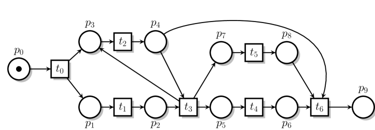
Figure 1: An example Petri net

A marking $m:P\to\mbox{${\mathbb{N}}$}$ maps a number of tokens to every place. A transition $t$ in $T$ is said enabled at $m$ if $m\geq\mathbf{Pre}(t)$. If enabled at $m$, transition $t$ may fire yielding a marking $m^{\prime}=m-\mathbf{Pre}(t)+\mathbf{Post}(t)$. This is written ${m\smash[t]{\stackrel{{\scriptstyle t}}{{\rightarrow}}}m^{\prime}}$, or simply $m\stackrel{{\scriptstyle}}{{\rightarrow}}m^{\prime}$ when only markings are of interest. Intuitively, places hold integers and together encode the state (or marking) of a net; transitions define state changes.

The reachability set, or state space, of $N$ is the set of markings $\mathcal{R}(N)=\{\,m\leavevmode\nobreak\ \mid\leavevmode\nobreak\ m_{0}\stackrel{{\scriptstyle*}}{{\rightarrow}}m\,\}$, where $\stackrel{{\scriptstyle*}}{{\rightarrow}}$ is the reflexive and transitive closure of $\stackrel{{\scriptstyle}}{{\rightarrow}}$.

A firing sequence $\sigma$ over $T$ is a sequence $t_{1},\dots,t_{n}$ of transitions in $T$ such that there are some markings $m_{1}\dots,m_{n+1}$ with $\smash[t]{m_{1}\stackrel{{\scriptstyle t_{1}}}{{\rightarrow}}m_{2}\land\dots\land m_{n}\stackrel{{\scriptstyle t_{n}}}{{\rightarrow}}m_{n+1}}$. This can be written $m_{1}\stackrel{{\scriptstyle\sigma}}{{\rightarrow}}m_{n+1}$. Its displacement, or marking change, is $\Delta(\sigma)=\Sigma_{i=1}^{n}(\mathbf{Post}(t_{i})-\mathbf{Pre}(t_{i}))$, where $\Delta:P\to\mbox{${\mathbb{Z}}$}$, and its hurdle $H(\sigma)$ is the smallest marking (pointwise) from which the sequence is firable.
Displacements (or marking changes) and hurdles are discussed in [8], where the existence and uniqueness of hurdles is proved. As an illustration, the displacement of sequence $t_{2}t_{5}t_{3}$ in the net Figure 1 is $\{(p_{2},-1),(p_{5},1),(p_{9},1)\}$ (and 0 for all other places, implicitly), its hurdle is $\{(p_{2},1),(p_{3},1),(p_{7},1)\}$.

The postset of a transition $t$ is $t^{\bullet}=\{\,p\mid\mathbf{Post}(t)(p)>0\,\}$, its preset is ${}^{\bullet}t=\{\,p\mid\mathbf{Pre}(t)(p)>0\,\}$. Symmetrically for places, $p^{\bullet}=\{\,t\mid\mathbf{Pre}(t)(p)>0\,\}$ and ${}^{\bullet}p=\{\,t\mid\mathbf{Post}(t)(p)>0\,\}$.

A net is ordinary if all its arcs have weight one; for all transition $t$ in $T$, and place $p$ in $P$, we have $\mathbf{Pre}(t)(p)\leq 1$ and $\mathbf{Post}(t)(p)\leq 1$. Otherwise it is said generalized.

A net $N$ is bounded if there is an (integer) bound $b$ such that $m(p)\leq b$ for all $m\in\mathcal{R}(N)$ and $p\in P$. The net is said safe when the bound is $1$. All nets considered in this paper are assumed bounded.

The net in Figure 1 is ordinary and safe. Its state space holds 14 markings.

3 The Reduction System

We describe our set of reduction rules using three main categories. For each category, we give a property that can be used to recover the state space of a net, after reduction, from that of the reduced net.

3.1 Removal of Redundant Transitions

A transition is redundant when its effects can always be achieved by firing instead an alternative sequence of transitions. Our definition of redundant transitions slightly strengthens that of bypass transitions in [15]. It is not fully structural either, but makes it easier to identify special cases structurally.

Definition 3.1 (Redundant transition).

Given a net $(P,T,\mathbf{Pre},\mathbf{Post},m_{0})$, a transition $t$ in $T$ is redundant if there is a firing sequence $\sigma$ over $T\setminus\{t\}$ such that $\Delta(t)=\Delta(\sigma)$ and $H(t)\geq H(\sigma)$. $\blacksquare$

There are special cases that do not require to explore combinations of transitions. This includes identity transitions, such that $\Delta(t)=0$, and duplicate transitions, such that for some other transition $t^{\prime}$ and integer $k$, $\Delta(t)=k.\Delta(t^{\prime})$. Finding redundant transitions using Definition 3.1 can be convenient too, provided the candidate $\sigma$ are restricted (e.g. in length). Figure 2 (left) shows some examples of redundant transitions. Clearly, removing a redundant transition from a net does not change its state space.

Theorem 3.1.

If net $N^{\prime}$ is the result of removing some redundant transition in net $N$ then $\mathcal{R}(N)=\mathcal{R}(N^{\prime})$

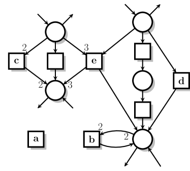
identity (a,b), duplicate (c) general redundant (d,e)

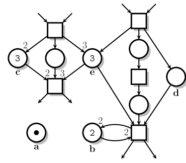
constant (a,b), duplicate (c) general redundant (d,e)

Figure 2: Some examples of redundant transitions (left) and places (right)

3.2 Removal of Redundant Places

A place is redundant if it never restricts the firing of its output transitions. Removing redundant places from a net preserves its language of firing sequences [3]. We wish to avoid enumerating marking for detecting such places, and further be able to recover the marking of a redundant place from those of the other places. For these reasons, our definition of redundant places is a slightly strengthened version of that of structurally redundant places in [3] (last clause is an equation).

Definition 3.2 (redundant place).

Given a net $(P,T,\mathbf{Pre},\mathbf{Post},m_{0})$, a place $p$ in $P$ is redundant if there is some set of places $I$ from $P\setminus\{p\}$, some valuation $v:(I\cup\{p\})\rightarrow(\mbox{${\mathbb{N}}$}-\{0\})$, and some constant $b\in\mbox{${\mathbb{N}}$}$ such that, for any $t\in T$:

1. The weighted initial marking of $p$ is not smaller than that of $I$:

   $b=v(p).m_{0}(p)-\Sigma_{q\in I}v(q).m_{0}(q)$

2. To fire $t$, the difference between its weighted precondition on $p$ and that on $I$ may not be larger than $b$: $v(p).\mathbf{Pre}(t)(p)-\Sigma_{q\in I}v(q).\mathbf{Pre}(t)(q)\leq b$

3. When $t$ fires, the weighted growth of the marking of $p$ is equal to that of $I$:

   $v(p).(\mathbf{Post}(t)(p)-\mathbf{Pre}(t)(p))=\Sigma_{q\in I}v(q).(\mathbf{Post}(t)(q)-\mathbf{Pre}(t)(q))$ $\blacksquare$

This definition can be rephrased as an integer linear programming problem [17], convenient in practice for computing redundant places in reasonably sized nets (say when $|P|\ \leq 50$). Like with redundant transitions, there are special cases that lead to easily identifiable redundant places. These are constant places—those for which set $I$ in the definition is empty—and duplicated places, when set $I$ is a singleton. Figure 2 (right) gives some examples of such places.

From Definition 3.2, we can show that the marking of a redundant place $p$ can always be computed from the markings of the places in $I$ and the valuation function $v$. Indeed, for any marking $m$ in $\mathcal{R}(N)$, we have $v(p).m(p)=\Sigma_{q\in I}v(q).m(q)+b$, where the constant $b$ derives from the initial marking $m_{0}$. Hence we have a relation $k_{p}.m(p)=\rho_{p}(m)$, where $k_{p}=v(p)$ and $\rho_{p}$ is some linear expression on the places of the net.

Theorem 3.2.

If $N^{\prime}$ is the result of removing some redundant place $p$ from net $N$, then there is an integer constant $k\in\mbox{${\mathbb{N}}$}^{*}$, and a linear expression $\rho$, such that, for all marking $m$: $m\cup\{(p,(1/k).\rho(m))\}\in\mathcal{R}(N)\Leftrightarrow m\in\mathcal{R}(N^{\prime})$.

3.3 Place Agglomerations

Conversely to the rules considered so far, place agglomerations do not preserve the number of markings of the nets they are applied to. They constitute the cornerstone of our reduction system; the purpose of the previous rules is merely to simplify the net so that agglomeration rules can be applied. We start by introducing a convenient notation.

Definition 3.3 (Sum of places).

A place $a$ is the sum of places $p$ and $q$, written $a=p\boxplus q$, if: $m_{0}(a)=m_{0}(p)+m_{0}(q)$ and, for all transition $t$, $\mathbf{Pre}(t)(a)=\mathbf{Pre}(t)(p)+\mathbf{Pre}(t)(q)$ and $\mathbf{Post}(t)(a)=\mathbf{Post}(t)(p)+\mathbf{Post}(t)(q)$. $\blacksquare$

Clearly, operation $\boxplus$ is commutative and associative. We consider two categories of place agglomeration rules; each one consisting in the simplification of a sum of places. Examples are shown in Fig. 3.

	$\rightarrow$
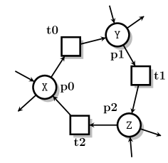
	$\rightarrow$

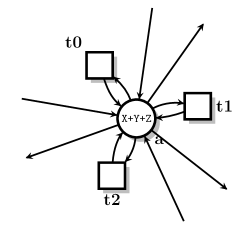
Figure 3: Agglomeration examples: chain (top), loop (for $n=3$, bottom)

Definition 3.4 (Chain agglomeration).

Given a net $(P,T,\mathbf{Pre},\mathbf{Post},m_{0})$, a pair of places $p$, $q$ in $P$ can be chain agglomerated if there is some $t\in T$ such that: ${}^{\bullet}t=\{p\}$; $t^{\bullet}=\{q\}$; $\mathbf{Pre}(t)(p)=\mathbf{Post}(t)(q)=1$; ${}^{\bullet}q=\{t\}$; and $m_{0}(q)=0$. Their agglomeration consists of replacing places $p$ and $q$ by a place $a$ equal to their sum: $a=p\boxplus q$. $\blacksquare$

Definition 3.5 (Loop agglomeration).

A sequence of $n$ places $(\pi_{i})_{i=0}^{n-1}$ can be loop agglomerated if the following condition is met:

$$(\forall i<n)(\exists t\in T)(\mathbf{Pre}(t)=\{(\pi_{i},1)\}\land\mathbf{Post}(t)=\{(\pi_{(i+1)(\text{mod}\ {n})},1)\})\leavevmode\nobreak\ .$$

Their agglomeration consists of replacing places $\pi_{0},\dots,\pi_{n-1}$ by a single place, $a$, defined as their sum: $a=\boxplus_{i=0}^{n-1}{\pi_{i}}$. $\blacksquare$

Clearly, whenever some place $a$ of a net obeys $a=p\boxplus q$ for some places $p$ and $q$ of the same net, then place $a$ is redundant in the sense of definition 3.2. The effects of agglomerations on markings are stated by Theorem 3.3.

Theorem 3.3.

Let $N$ and $N^{\prime}$ be the nets before and after agglomeration of some set of places $A$ as place $a$. Then for all markings $m$ over $(P\setminus A)$ and $m^{\prime}$ over $A$ we have: $(m\cup m^{\prime})\in\mathcal{R}(N)\Leftrightarrow m\cup\{(a,\Sigma_{p\in A}m^{\prime}(p)\}\in\mathcal{R}(N^{\prime})$.

Proof.

Assume $N$ is a net with set of places $P$. Let us first consider the case of the chain agglomeration rule in Fig. 3 (top). We have to prove that for all marking $m$ of $P\setminus\{p,q\}$ and for all values $x,y$ in ${\mathbb{N}}$:

$$m\cup\{(p,x),(q,y)\}\in\mathcal{R}(N)\Leftrightarrow m\cup\{(a,x+y)\}\in\mathcal{R}(N^{\prime})$$

Left to right (L): Let $N^{+}$ be net $N$ with place $a=p\boxplus q$ added. Clearly, $a$ is redundant in $N^{+}$, with $v(a)=v(p)=v(q)=1$. So $N$ and $N^{+}$ admit the same firing sequences, and for any $m\in\mathcal{R}(N^{+})$, we have $m(a)=m(p)+m(q)$. Next, removing places $p$ and $q$ from $N^{+}$ (the result is net $N^{\prime}$) can only relax firing constraints, hence any $\sigma$ firable in $N^{+}$ (and thus in $N$) is also firable in $N^{\prime}$, which implies the goal.

Right to left (R): we use two intermediate properties ($\forall m,x,u,v$ implicit). We write $m\sim m^{\prime}$ when $m$ and $m^{\prime}$ agree on all places except $p$, $q$ and $a$, and $m\approx m^{\prime}$ when $m\sim m^{\prime}\land m(p)=m^{\prime}(a)\land m(q)=0$.

Property (1): $m\cup\{(a,x)\}\in\mathcal{R}(N^{\prime})\Rightarrow m\cup\{(p,x),(q,0)\}\in\mathcal{R}(N)$.

Since $\Delta(t)=0$, any marking reachable in $N^{\prime}$ is reachable by a sequence not containing $t$, call these sequences $t$-free. Property (1) follows from a simpler relation, namely (Z): whenever $m\approx m^{\prime}$ ($m\in\mathcal{R}(N)$, $m^{\prime}\in\mathcal{R}(N^{\prime})$) and $\smash[t]{m^{\prime}\stackrel{{\scriptstyle\delta}}{{\rightarrow}}w^{\prime}}$, ($\delta$ $t$-free), then there is a sequence $\omega$ such that $m\stackrel{{\scriptstyle\omega}}{{\rightarrow}}w$ and $w\approx w^{\prime}$.

Any $t$-free sequence firable in $N^{\prime}$ but not in $N$ can be written $\sigma.t^{\prime}.\gamma$, where $\sigma$ is firable in $N$ and transition $t^{\prime}$ is not firable in $N$ after $\sigma$. Let $w$, $w^{\prime}$ be the markings reached by $\sigma$ in $N$ and $N^{\prime}$, respectively. Since $\sigma$ is firable in $N$, we have $w\approx w^{\prime}$, by (L) and the fact that $\sigma$ is $t$-free (only $t$ can put tokens in $q$). That $t^{\prime}$ is not firable at $w$ but firable at $w^{\prime}$ is only possible if $t^{\prime}$ is some output transition of $a$ since $w\sim w^{\prime}$ and the preconditions of all other transitions of $N^{\prime}$ than $a$ are identical in $N$ and $N^{\prime}$. That is, $t^{\prime}$ must be an output transition of either or both $p$ or $q$ in $N$. If $t^{\prime}$ has no precondition on $q$ in $N$, then it ought to be firable at $w$ in $N$ since $w(p)=w^{\prime}(a)$. So $t^{\prime}$ must have a precondition on $q$; we have $w(q)\not\geq\mathbf{Pre}(t^{\prime})(q)$ in $N$ and $w^{\prime}(a)\geq\mathbf{Pre}^{\prime}(t^{\prime})(a)$ in $N^{\prime}$. Therefore, we can fire transition $t$ $n$ times from $w$ in $N$, where $n=\mathbf{Pre}(t^{\prime})(q)$, since $w^{\prime}(a)=w(p)$ and $t^{\prime}$ is enabled at $w^{\prime}$, and this leads to a marking enabling $t^{\prime}$. Further, firing $t^{\prime}$ at that marking leaves place $q$ in $N$ empty since only transition $t$ may put tokens in $q$. Then the proof of Property (1) follows from (Z) and the fact that Definition 3.4 ensures $m_{0}\approx m_{0}^{\prime}$.

Property (2): if $m\cup\{(p,x),(q,0)\}\in\mathcal{R}(N)$ and $(u+v=x)$ then $m\cup\{(p,u),(q,v)\}\in\mathcal{R}(N)$.

Obvious from Definition 3.4: the tokens in place $p$ can be moved one by one into place $q$ by firing $t$ in sequence $v$ times.

Combining Property (1) and (2) is enough to prove (R), which completes the proof for chain agglomerations. The proof for loop agglomerations is similar.∎

3.4 The Reduction System

The three categories of rules introduced in the previous sections constitute the core of our reduction system. Our implementation actually adds to those a few special purpose rules. We mention three examples of such rules here, because they play a significant role in the experimental results of Sect. 7, but without technical details. These rules are useful on nets generated from high level descriptions, that often exhibit translation artifacts like dead transitions or source places.

The first extra rule is the dead transition removal rule. It is sometimes possible to determine statically that some transitions of a net are never firable. A fairly general rule for identifying statically dead transitions is proposed in [5]. Removal of statically dead transitions from a net has no effects on its state space.

A second rule allows us to remove a transition $t$ from a net $N$ when $t$ is the sole transition enabled in the initial marking and $t$ is firable only once. Then, instead of counting the markings reachable from the initial marking of the net, we count those reachable from the output marking of $t$ in $N$ and add 1. Removing such transitions often yields structurally simpler nets.

Our last example is an instance of simple rules that can be used to do away with very basic (sub-)nets, containing only a single place. This is the case, for instance, of the source-sink nets defined below. These rules are useful if we want to fully reduce a net. We say that a net is totally reduced when its set of places and transitions are empty ($P=T=\emptyset$).

Definition 3.6 (Source-sink pair).

A pair $(p,t)$ in net $N$ is a source-sink pair if ${}^{\bullet}p=\emptyset$, $p^{\bullet}=\{t\}$, $\mathbf{Pre}(t)=\{(p,1)\}$ and $\mathbf{Post}(t)=\emptyset$. $\blacksquare$

Theorem 3.4 (Source-sink pairs).

If $N^{\prime}$ is the result of removing a source-sink pair $(p,t)$ in net $N$ then $(\forall z\leq m_{0}(p))(\forall m)(m\cup\{(p,z)\}\in\mathcal{R}(N)\Leftrightarrow m\in\mathcal{R}(N^{\prime}))$.

Omitting for the sake of clarity the first two extra rules mentioned above, our final reduction system resumes to removal of redundant transitions (referred to as the T rule) and of redundant places (R rule), agglomeration of places (A rules) and removal of source-sink pairs (L rule).

Rules T have no effects on markings. For the other three rules, the effect on the markings can be captured by an equation or an inequality. These have shape $v_{p}.m(p)=\sum_{q\neq p}v_{q}.m(q)+b$ for redundant places, where $b$ is a constant, shape $m(a)=\Sigma_{p\in A}m(p)$ for agglomerations, and shape $m(p)\leq k$ for source-sink pairs, where $k$ is some constant. In all these equations, the terms $m(q)$ are marking variables; variable $m(q)$ is associated with the marking of place $q$. For readability, we will often use the name of the place instead of its associated marking variable. For instance, the marking equation $2.m(p)=3.m(q)+4$, resulting from a (R) rule, would be simply written $2.p=3.q+4$.

We show in Sect. 5 that the state space of a net can be reconstructed from that of its reduced net and the set of (in)equalities collected when a rule is applied. Before considering this result, we illustrate the effects of reductions on a full example.

4 An Illustrative Example — HouseConstruction

.

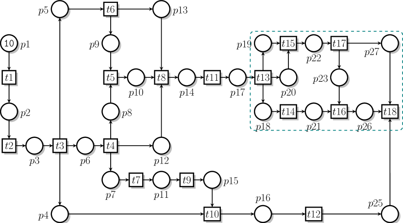
Figure 4: HouseConstruction-10 example net

We take as example a model provided in the Model Checking Contest (MCC, http://mcc.lip6.fr), a recurring competition of model-checking tools [6]. This model is a variation of a Petri net model found in [14], which is itself derived from the PERT chart of the construction of a house found in [11]. The model found in the MCC collection, reproduced in Fig. 4, differs from that of [14] in that it omits time constraints and a final sink place. In addition, the net represents the house construction process for a number of houses simultaneously rather than a single one. The number of houses being built is represented by the marking of place $p_{1}$ of the net ($10$ in the net represented in Fig. 4).

We list in Fig. 5 a possible reduction sequence for our example net, one for each line. To save space, we have omitted the removal of redundant transitions. For each reduction, we give an indication of its kind (R, A, …), the marking equation witnessing the reduction, and a short description. The first reduction, for instance, says that place $p_{19}$ is removed, being a duplicate of place $p_{20}$. At the second step, places $p11$ and $p7$ are agglomerated as place $a1$, a “fresh” place not found in the net yet.

R |- p19 = p20 p19 duplicate A |- a1 = p11 + p7 agglomeration A |- a2 = p17 + p14 agglomeration A |- a3 = p2 + p1 agglomeration A |- a4 = p21 + p18 agglomeration A |- a5 = p22 + p20 agglomeration A |- a6 = p25 + p16 agglomeration A |- a7 = p15 + a1 agglomeration A |- a8 = p3 + a3 agglomeration R |- p12 = p10 + p8 p12 redundant R |- p13 = p10 + p9 p13 redundant R |- a4 = a5 + p23 a4 redundant R |- p27 = p23 + p26 p27 redundant

R |- p4 = p6 + a7 p4 redundant A |- a9 = a2 + p10 agglomeration A |- a10 = a6 + a7 agglomeration A |- a11 = p23 + a5 agglomeration A |- a12 = p9 + p5 agglomeration A |- a13 = a11 + p26 agglomeration A |- a14 = a13 + a9 agglomeration R |- a12 = p6 + p8 a12 redundant R |- a10 = a14 + p8 a10 redundant A |- a15 = a14 + p8 agglomeration A |- a16 = p6 + a8 agglomeration A |- a17 = a15 + a16 agglomeration L |- a17 <= 10 a17 source

Figure 5: Reduction traces for net HouseConstruction-10

Each reduction is associated with an equation or inequality linking the markings of the net before and after application of a rule. The system of inequalities gathered is shown below, with agglomeration places $a_{i}$ eliminated. We show in the next section that the set of solutions of this system, taken as markings, is exactly the set of reachable markings of the net.

$$\begin{array}[]{c}\begin{array}[]{rcl@{~~~~~~~~~~~~~~~~}rcl}p19&=&p20\hfil\leavevmode\nobreak\ \leavevmode\nobreak\ \leavevmode\nobreak\ \leavevmode\nobreak\ \leavevmode\nobreak\ \leavevmode\nobreak\ \leavevmode\nobreak\ \leavevmode\nobreak\ \leavevmode\nobreak\ \leavevmode\nobreak\ \leavevmode\nobreak\ \leavevmode\nobreak\ \leavevmode\nobreak\ \leavevmode\nobreak\ \leavevmode\nobreak\ \leavevmode\nobreak\ &p4&=&p6+p15+p11+p7\\ p12&=&p10+p8\hfil\leavevmode\nobreak\ \leavevmode\nobreak\ \leavevmode\nobreak\ \leavevmode\nobreak\ \leavevmode\nobreak\ \leavevmode\nobreak\ \leavevmode\nobreak\ \leavevmode\nobreak\ \leavevmode\nobreak\ \leavevmode\nobreak\ \leavevmode\nobreak\ \leavevmode\nobreak\ \leavevmode\nobreak\ \leavevmode\nobreak\ \leavevmode\nobreak\ \leavevmode\nobreak\ &p9+p5&=&p6+p8\\ p13&=&p10+p9\hfil\leavevmode\nobreak\ \leavevmode\nobreak\ \leavevmode\nobreak\ \leavevmode\nobreak\ \leavevmode\nobreak\ \leavevmode\nobreak\ \leavevmode\nobreak\ \leavevmode\nobreak\ \leavevmode\nobreak\ \leavevmode\nobreak\ \leavevmode\nobreak\ \leavevmode\nobreak\ \leavevmode\nobreak\ \leavevmode\nobreak\ \leavevmode\nobreak\ \leavevmode\nobreak\ &p21+p18&=&p22+p20+p23\\ p27&=&p23+p26\hfil\leavevmode\nobreak\ \leavevmode\nobreak\ \leavevmode\nobreak\ \leavevmode\nobreak\ \leavevmode\nobreak\ \leavevmode\nobreak\ \leavevmode\nobreak\ \leavevmode\nobreak\ \leavevmode\nobreak\ \leavevmode\nobreak\ \leavevmode\nobreak\ \leavevmode\nobreak\ \leavevmode\nobreak\ \leavevmode\nobreak\ \leavevmode\nobreak\ \leavevmode\nobreak\ &\end{array}\\ \vspace{-6pt}\begin{array}[]{rcl}p25+p16+p15+p11+p7&=&p26+p23+p22+p20+p17+p14+p10+p8\\ p26+p23+p22+p20+p17&+&p14+p10+p8+p6+p3+p2+p1\leq 10\\ \end{array}\\ \end{array}$$

This example is totally reduced using the sequence of reductions listed. And we have found other examples of totally reducible net in the MCC benchmarks. In the general case, our reduction system is not complete; some nets may be only partially reduced, or not at all.

When a net is only partially reducible, the inequalities, together with an explicit or logic-based symbolic description of the reachability set of the residual net, yield a hybrid representation of the state space of the initial net. Such hybrid representations are still suitable for model checking reachability properties or counting markings.

Order of application of reduction rules. Our reduction system does not constrain the order in which reductions are applied. Our tool attempts to apply them in an order that minimizes reduction costs.

The rules can be classified into “local” rules, detecting some structural patterns on the net and transforming them, like removal of duplicate transitions or places, or chain agglomerations, and ‘’non-local” rules, like removal of redundant places in the general case (using integer programming). Our implementation defers the application of the non-local rules until no more local rule can be applied. This decreases the cost of non-local reductions as they are applied to smaller nets.

Another issue is the confluence of the rules. Our reduction system is not confluent: different reduction sequences for the same net could yield different residual nets. This follows from the fact that agglomeration rules do not preserve in general the ordinary character of the net (that all arcs have weight 1), while agglomeration rules require that the candidate places are connected by arcs of weight 1 to the same transition.

An example net exhibiting the problem is shown in Fig. 6(a). Agglomeration of places $p3$ and $p4$ in this net, followed by removal of identity transitions, yields the net in Fig. 6(b). Place $a1$ in the reduced net is the result of agglomerating $p3$ and $p4$; this is witnessed by equation $a1=p3+p4$. Note that the arcs connecting place $a1$ to transitions $t0$ and $t1$ both have weight 2.

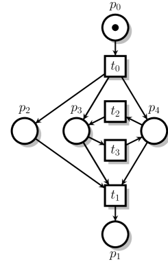
(a)

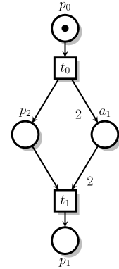
(b)

Figure 6: Non confluence example

Next, place $p2$ in the reduced net is a duplicate of place $a1$, according to the definitions of Sect. 3.2, the corresponding equation is $2.p2=a1$. But, from the same equation, $a1$ is a duplicate of $p2$ as well. But removing $p2$ or $a1$ have differents effects:

• If $a1$ is removed, then we can fully reduce the net by the following sequence of reductions:

  A |- a2 = p1 + p2	agglomeration
  A |- a3 = a2 + p0	agglomeration
  R |- a3 = 1	constant place

• If $p2$ is removed instead, then the resulting net cannot be reduced further: places $p0$, $a1$ and $p1$ cannot be agglomerated because of the presence of arcs with weight larger than 1.

Confluence of the system could be easily obtained by restricting the agglomeration rules so that no arcs with weight larger than 1 could be produced. But it is more effective to favour the expressiveness of our reduction rules.

Alternatively, agglomeration rules could be generalized to handle arbitrary weights on the arcs linking the agglomerated places; this is a scheduled improvement of our reduction system.

5 Correctness of Markings Reconstruction

We prove that we can reconstruct the markings of an (initial) net, before application of a rule, from that of the reduced net. This property ensues from the definition of a net-abstraction relation, defined below.

We start by defining some notations useful in our proofs. We use $\mathcal{U},\mathcal{V},\dots$ for finite sets of non-negative integer variables. We use $Q,Q^{\prime}$ for systems of linear equations (and inequalities) and the notation $\mathbf{V}(Q)$ for the set of variables occurring in $Q$. The system obtained by concatenating the relations in $Q_{1}$ and $Q_{2}$ is denoted $(Q_{1};Q_{2})$ and the “empty system” is denoted $\emptyset$.

A valuation $e$ of $\mbox{${\mathbb{N}}$}^{\mathcal{V}}$ is a solution of $Q$, with $\mathcal{V}=\mathbf{V}(Q)$, if all the relations in $Q$ are (trivially) valid when replacing all variables $x$ in $\mathcal{V}$ by their value $e(x)$. We denote $\langle Q\rangle$ the subset of $\mbox{${\mathbb{N}}$}^{\mathbf{V}(Q)}$ consisting in all the solutions of $Q$.

If $E\subseteq\mbox{${\mathbb{N}}$}^{\mathcal{V}}$ then $E\downarrow\mathcal{U}$ is the projection of $E$ over variables $\mathcal{U}$, that is the subset of $\mbox{${\mathbb{N}}$}^{\mathcal{U}}$ obtained from $E$ by restricting the domain of its elements to $\mathcal{U}$. conversely, we use $E\uparrow\mathcal{U}$ to denote the lifting of $E$ to $\mathcal{U}$, that is the largest subset $E^{\prime}$ of $\mbox{${\mathbb{N}}$}^{\mathcal{U}}$ such that $E^{\prime}\downarrow\mathcal{V}=E$.

Definition 5.1 (Net-abstraction).

A triple $(N_{1},Q,N_{2})$ is a net-abstraction, or simply an abstraction, if $N_{1}$, $N_{2}$ are nets with respective sets of places $P_{1}$, $P_{2}$ (we may have $P_{1}\cap P_{2}\not=\emptyset)$, $Q$ is a linear system of equations, and:

$$\mathcal{R}(N_{1})=\left((\mathcal{R}(N_{2})\uparrow\mathcal{V})\cap(\langle Q\rangle\uparrow\mathcal{V})\right)\downarrow P_{1}\qquad\text{where }\mathcal{V}=\mathbf{V}(Q)\cup P_{1}\cup P_{2}\leavevmode\nobreak\ .$$

Intuitively, $N_{2}$ is an abstraction of $N_{1}$ (through $Q$) if, from every reachable marking $m\in\mathcal{R}(N_{2})$, the markings obtained from solutions of $Q$—restricted to those solutions such that $x=m(x)$ for all “place variable” $x$ in $P_{2}$—are always reachable in $N_{1}$. The definition also entails that all the markings in $\mathcal{R}(N_{1})$ can be obtained this way.

Theorem 5.1 (Net-abstractions from reductions).

For any nets $N$, $N_{1}$, $N_{2}$:

1. $(N,\emptyset,N)$ is an abstraction;

2. If $(N_{1},Q,N_{2})$ is an abstraction then $(N_{1},Q^{\prime},N_{3})$ is an abstraction if either:

   • $Q^{\prime}=Q$ and $N_{3}$ is obtained from $N_{2}$ by removing a redundant transition (see Sect. 3.1);

   • $Q^{\prime}=(Q;k.p=l)$ and $N_{3}$ is obtained from $N_{2}$ by removing a redundant place $p$ and $k.p=l$ is the associated marking equation (see Sect. 3.2);

   • $Q^{\prime}=(Q;a=\Sigma_{p\in A}(p))$, where $a\not\in\mathbf{V}(Q)$ and $N_{3}$ is obtained from $N_{2}$ by agglomerating the places in $A$ as a new place, $a$ (see Sect. 3.3);

   • $Q^{\prime}=(Q;p\leq k)$ and $N_{3}$ is obtained from $N_{2}$ by removal of a source-sink pair $(p,t)$ with $m_{0}(p)=k$ (see Sect. 3.4).

Proof.

Property (1) is obvious from Definition 5.1. Property (2) is proved by case analysis. First, let $\mathcal{V}=\mathbf{V}(Q)\cup P_{1}\cup P_{2}$ and $\mathcal{U}=\mathcal{V}\cup P_{3}$ and notice that for all candidate $(N_{1},Q^{\prime},N_{3})$ we have $\mathbf{V}(Q^{\prime})\cup P_{1}\cup P_{3}=\mathcal{U}$. Then, in each case, we know $(H):\mathcal{R}(N_{1})=(\mathcal{R}(N_{2})\uparrow\mathcal{V}\cap\langle Q\rangle\uparrow\mathcal{V})\downarrow P_{1}$ and we must prove $(G):\mathcal{R}(N_{1})=(\mathcal{R}(N_{3})\uparrow\mathcal{U}\cap\langle Q^{\prime}\rangle\uparrow\mathcal{U})\downarrow P_{1}$.

Case (T) : $Q^{\prime}=Q$. By Th. 3.1, we have $P_{3}=P_{2}$, hence $\mathcal{V}=\mathcal{U}$, and $\mathcal{R}(N_{3})=\mathcal{R}(N_{2})$. Replacing $\mathcal{R}(N_{2})$ by $\mathcal{R}(N_{3})$ and $\mathcal{V}$ by $\mathcal{U}$ in (H) yields (G).

Case (R) : By Th. 3.2 we have : $\mathcal{R}(N_{2})=\mathcal{R}(N_{3})\uparrow P_{2}\cap\langle k.p=l\rangle\uparrow P_{2}$. replacing $\mathcal{R}(N_{2})$ by this value in $(H)$ yields $\mathcal{R}(N_{1})=((\mathcal{R}(N_{3})\uparrow P_{2}\cap\langle k.p=l\rangle\uparrow P_{2})\uparrow\mathcal{V}\cap\langle Q\rangle\uparrow\mathcal{V})\downarrow P_{1}$. Since $P_{2}\subseteq\mathcal{V}$, we may safely lift to $\mathcal{V}$ instead of $P_{2}$, so: $\mathcal{R}(N_{1})=(\mathcal{R}(N_{3})\uparrow\mathcal{V}\cap\langle k.p=l\rangle\uparrow\mathcal{V}\cap\langle Q\rangle\uparrow\mathcal{V})\downarrow P_{1}$. Which is equivalent to: $\mathcal{R}(N_{1})=(\mathcal{R}(N_{3})\uparrow\mathcal{V}\cap\langle Q;k.p=l\rangle\uparrow\mathcal{V})\downarrow P_{1}$, and equal to (G) since $P_{3}\subseteq\mathcal{V}$ and $Q^{\prime}=(Q;k.p=l)$.

Case (A): Let $S_{p}$ denotes the value $\Sigma_{p\in A}(p)$. By Th. 3.3 we have: $\mathcal{R}(N_{2})=(\mathcal{R}(N_{3})\uparrow(P_{2}\cup P_{3})\cap\langle a=S_{p}\rangle\uparrow(P_{2}\cup P_{3}))\downarrow P_{2}$. Replacing $\mathcal{R}(N_{2})$ by this value in $(H)$ yields: $\mathcal{R}(N_{1})=(((\mathcal{R}(N_{3})\uparrow(P_{2}\cup P_{3})\cap\langle a=S_{p}\rangle\uparrow(P_{2}\cup P_{3}))\downarrow P_{2})\uparrow\mathcal{V}\cap\langle Q\rangle\uparrow\mathcal{V})\downarrow P_{1}$. Instead of $\mathcal{V}$, we may lift to $\mathcal{U}$ since $\mathcal{U}=\mathcal{V}\cup\{a\}$, $a\not\in\mathbf{V}(Q)$ and $a\not\in P_{1}$, so: $\mathcal{R}(N_{1})=(((\mathcal{R}(N_{3})\uparrow(P_{2}\cup P_{3})\cap\langle a=S_{p}\rangle\uparrow(P_{2}\cup P_{3}))\downarrow P_{2})\uparrow\mathcal{U}\cap\langle Q\rangle\uparrow\mathcal{U})\downarrow P_{1}$. Projection on $P_{2}$ may be omitted since $P_{2}\cup P_{3}=P_{2}\cup\{a\}$ and $a\not\in\mathbf{V}(Q)$, leading to:

$\mathcal{R}(N_{1})=((\mathcal{R}(N_{3})\uparrow(P_{2}\cup P_{3})\cap\langle a=S_{p}\rangle\uparrow(P_{2}\cup P_{3}))\uparrow\mathcal{U}\cap\langle Q\rangle\uparrow\mathcal{U})\downarrow P_{1}$.

Since $P_{2}\cup P_{3}\subseteq\mathcal{U}$, this is equivalent to: $\mathcal{R}(N_{1})=(\mathcal{R}(N_{3})\uparrow\mathcal{U}\cap\langle a=S_{p}\rangle\uparrow\mathcal{U}\cap\langle Q\rangle\uparrow\mathcal{U})\downarrow P_{1}$. Grouping equations yields: $\mathcal{R}(N_{1})=(\mathcal{R}(N_{3})\uparrow\mathcal{U}\cap\langle Q;a=S_{p}\rangle\uparrow\mathcal{U})\downarrow P_{1}$, which is equal to (G) since $Q^{\prime}=(Q;a=S_{p})$.

case (L): The proof is similar to that of case (R) and is based on the relation $\mathcal{R}(N_{2})=\mathcal{R}(N_{3})\uparrow P_{2}\cap\langle p\leq k\rangle\uparrow P_{2}$, obtained from Th. 3.4. ∎

Theorem 5.1 states the correctness of our reduction systems, since we can compose reductions sequentially and always obtain a net-abstraction. In particular, if a net $N$ is fully reducible, then we can derive a system of linear equations $Q$ such that $(N,Q,\emptyset)$ is a net-abstraction. In this case the reachable markings of $N$ are exactly the solutions of $Q$, projected on the places of $N$. If the reduced net, say $N_{r}$, is not empty then each marking $m\in\mathcal{R}(N_{r})$ represents a set of markings $\langle Q\rangle_{m}\subset\mathcal{R}(N)$: the solution set of $Q$ in which the places of the residual net are constrained as in $m$, and then projected on the places of $N$. Moreover the family of sets $\{\,\langle Q\rangle_{m}\leavevmode\nobreak\ \mid\leavevmode\nobreak\ m\in\mathcal{R}(N_{r})\}$ is a partition of $\mathcal{R}(N)$.

6 Counting Markings

We consider the problem of counting the markings of a net $N$ from the set of markings of the residual net $N_{r}$ and the (collected) system of linear equations $Q$. For totally reduced nets, counting the markings of $N$ resumes to that of counting the number of solutions in non negative integer variables of system $Q$. For partially reduced nets, a similar process must be iterated over all markings $m$ reachable in $N_{r}$ (a better implementation will be discussed shortly).

Available methods. Counting the number of integer solutions of a linear system of equations (inequalities can always be represented by equations by the addition of slack variables) is an active area of research.

A method is proposed in [1], implemented in the tool Azove, for the particular case where variables take their values in $\{0,1\}$. The method consists of building a Binary Decision Diagram for each equation, using Shannon expansion, and then to compute their conjunction (this is done with a specially tailored algorithm). The number of paths of the BDD gives the expected result. Our experiments with Azove show that, although the tool can be fast, its performances on larger system heavily depend on the ordering chosen for the BDD variables, a typical drawback of decision diagram based techniques. In any case, its usage in our context would be limited to safe nets.

For the general case, the current state of the art can be found in the work of De Loera et al. [12, 13] on counting lattice points in convex polytopes. Their approach is implemented in a tool called LaTTe; it relies on algebraic and geometric methods; namely the use of rational functions and the decomposition of cones into unimodular cones. Our experiments with LaTTe show that it can be conveniently used on systems with, say, less than $50$ variables. For instance, LaTTe is strikingly fast (less than $1$s) at counting the number of solutions of the system computed in Sect. 4. Moreover, its running time does not generally depend on the constants found in the system. As a consequence, computing the reachability count for $10$ or, say, $10^{12}$ houses takes exactly the same time.

An ad-hoc method. Though our experiments with LaTTe suffice to show that these approaches are practicable, we implemented our own counting method. Its main benefits over LaTTe, important for practical purposes, are that it can handle systems with many variables (say thousands), though it can be slower than LaTTe on small systems. Another reason for finding an alternative to LaTTe is that it provides no builtin support for parameterized systems, that is in the situation where we need to count the solutions of many instances of the same linear system differing only by some constants.

Our solution takes advantage of the stratified structure of the systems obtained from reductions, and it relies on combinatorial rather than geometric methods. While we cannot describe this tool in full details, we illustrate our approach and the techniques involved on a simple example.

Consider the system of equations obtained from the PN corresponding to the dashed zone of Fig. 4. This net consists of places in the range $p_{18}$—$p_{27}$ and is reduced by our system to a single place, $a_{13}$. The subset of marking equations related to this subnet is:

$$\begin{array}[]{l@{\hspace{6em}}l}R\vdash p_{19}=p_{20}\hfil\hskip 60.00009pt&R\vdash p_{27}=p_{23}+p_{26}\\ A\vdash a_{4}=p_{21}+p_{18}\hfil\hskip 60.00009pt&A\vdash a_{11}=p_{23}+a_{5}\\ A\vdash a_{5}=p_{22}+p_{20}\hfil\hskip 60.00009pt&A\vdash a_{13}=a_{11}+p_{26}\\ R\vdash a_{4}=a_{5}+p_{23}\hfil\hskip 60.00009pt\\ \end{array}\hskip 40.00006pt(Q)$$

Assume place $a_{13}$ is marked with $n$ tokens. Then, by Th. 5.1, the number of markings of the original net corresponding with marking $a_{13}=n$ in the reduced net is the number of non-negative integer solutions to system $(Q,a_{13}=n)$. Let us define the function $A_{13}:\mbox{${\mathbb{N}}$}\longrightarrow\mbox{${\mathbb{N}}$}$ that computes that number.

We first simplify system $(Q)$. Note that no agglomeration is involved in the redundancy (R) equations for $p_{19}$ and $p_{27}$, so these equations have no effects on the marking count and can be omitted. After elimination of variable $a_{5}$ and some rewriting, we obtain the simplified system $(Q^{\prime})$:

$$\begin{array}[]{l@{\hspace{6em}}l}A\vdash a_{4}=p_{21}+p_{18}\hfil\hskip 60.00009pt&R\vdash a_{4}=a_{11}\\ A\vdash a_{11}=p_{23}+p_{22}+p_{20}\hfil\hskip 60.00009pt&A\vdash a_{13}=a_{11}+p_{26}\end{array}\hskip 40.00006pt(Q^{\prime})$$

Let $(\!({k})\!)({x})$ denote the expression ${x+k-1}\choose{k-1}$, which denotes the number of ways to put $x$ tokens into $k$ slots. The first equation is $a_{4}=p_{21}+p_{18}$. If $a_{4}=x$, its number of solutions is $(\!({2})\!)({x})=x+1$. The second equation is $a_{11}=p_{23}+p_{22}+p_{20}$. If $a_{11}=x$, its number of solutions is $(\!({3})\!)({x})=\frac{(x+2)(x+1)}{2}$.

Now consider the system consisting of the first two equations and the redundancy equation $a_{4}=a_{11}$. If $a_{11}=x$, its number of solutions is $(\!({2})\!)({x})\times(\!({3})\!)({x})$ (the variables in both equations being disjoint). Finally, by noticing that $a_{11}$ can take any value between $0$ and $n$, we get:

$\displaystyle A_{13}(n)=\sum_{a_{11}=0}^{n}(\!({2})\!)({a_{11}})\times(\!({3})\!)({a_{11}})$

This expression is actually a polynomial, namely $\frac{1}{8}n^{4}+\frac{11}{12}n^{3}+\frac{19}{8}n^{2}+\frac{31}{12}n+1$.
By applying the same method to the whole net of Fig. 4, we obtain an expression involving six summations, which can be reduced to the following 18th-degree polynomial in the variable $X$ denoting the number of tokens in place $p_{1}$.

$${\scriptscriptstyle\begin{split}\tfrac{11}{19401132441600}X^{18}+\tfrac{1}{16582164480}X^{17}+\tfrac{2491}{836911595520}X^{16}+\tfrac{1409}{15567552000}X^{15}\\ {}+\tfrac{3972503}{2092278988800}X^{14}+\tfrac{161351}{5535129600}X^{13}+\tfrac{32745953}{96566722560}X^{12}+\tfrac{68229017}{22353408000}X^{11}\\ {}+\tfrac{629730473}{29262643200}X^{10}+\tfrac{83284643}{696729600}X^{9}+\tfrac{3063053849}{5852528640}X^{8}+\tfrac{74566847}{41472000}X^{7}\\ {}+\tfrac{1505970381239}{313841848320}X^{6}+\tfrac{32809178977}{3353011200}X^{5}+\tfrac{259109541797}{17435658240}X^{4}+\tfrac{41924892461}{2594592000}X^{3}\\ {}+\tfrac{4496167537}{381180800}X^{2}+\tfrac{62925293}{12252240}X^{1}+1\end{split}}$$

In the general case of partially reduced nets, the computed polynomial is a multivariate polynomial with at most as many variables as places remaining in the residual net. When that number of variables is too large, the computation of the final polynomial is out of reach, and we only make use of the intermediate algebraic term.

7 Computing Experiments

We integrated our reduction system and counting method with a state space generation tool, tedd, in the framework of our TINA toolbox for analysis of Petri nets [4] (www.laas.fr/tina). Tool tedd makes use of symbolic exploration and stores markings in a Set Decision Diagram [19]. For counting markings in presence of agglomerations, one has the choice between using the external tool LaTTe or using our native counting method discussed in Sect. 6.

Benchmarks. Our benchmark is constituted of the full collection of Petri nets used in the Model Checking Contest [6, 9]. It includes $627$ nets, organized into $82$ classes (simply called models). Each class includes several nets (called instances) that typically differ by their initial marking or by the number of components constituting the net. The size of the nets vary widely, from $9$ to $50\,000$ places, $7$ to $200\,000$ transitions, and $20$ to $1\,000\,000$ arcs. Most nets are ordinary (arcs have weight $1$) but a significant number are generalized nets. Overall, the collection provides a large number of PN with various structural and behavioral characteristics, covering a large variety of use cases.

Reduction ratio and prevalence. Our first results are about how well the reductions perform. We provide two different reduction strategies: compact, that applies all reductions described in Sect. 3, and clean, that only applies removal of redundant places and transitions. The reduction ratios on number of places (number of places before and after reduction) for all the MCC instances are shown in Fig. 7, sorted in descending order. We overlay the results for our two reduction strategies (the lower, in light color, for clean and the upper, in dark, for compact). We see that the impact of strategy clean alone is minor compared to compact. Globally, Fig. 7 shows that reductions have a significant impact on about half the models, with a very high impact on about a quarter of them. In particular, there is a surprisingly high number of models that are totally reducible by our approach (about $19$% of the models are fully reducible).

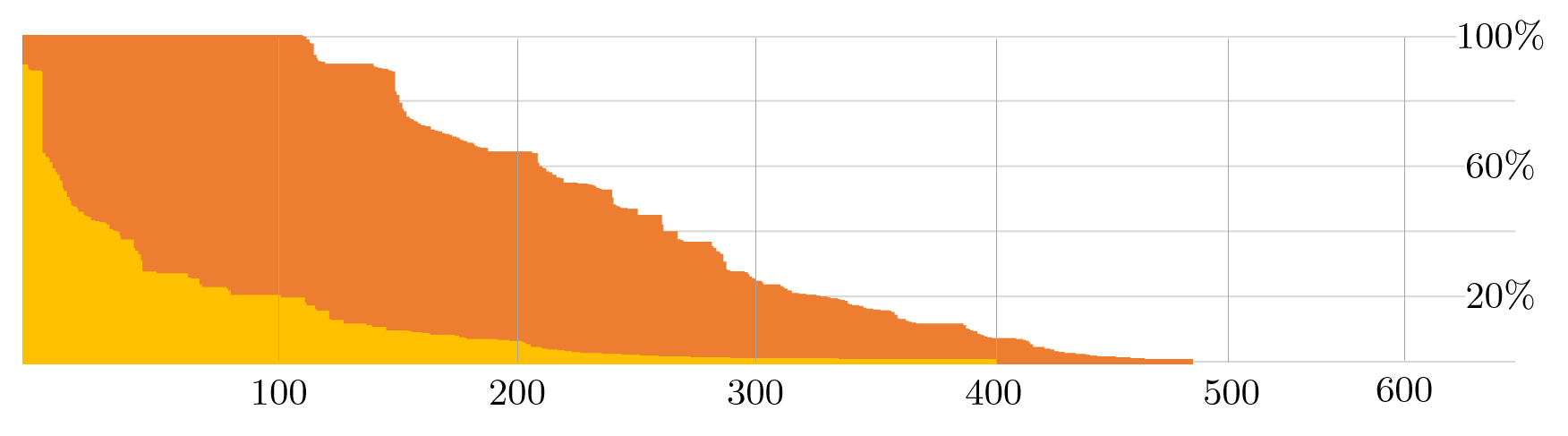
Figure 7: Distribution of reduction ratios (place count) over the $627$ PN instances.

Computing time of reductions. Many of the reduction rules implemented have a cost polynomial in the size of the net. The rule removing redundant places in the general case is more complex as it requires to solve an integer programming problem. For this reason we limit its application to nets with less than $50$ places. With this restriction, reductions are computed in a few seconds in most cases, and in about $3$ minutes for the largest nets. The restriction is necessary but, because of it, we do not reduce some nets that would be fully reducible otherwise.

Impact on the marking count problem. In our benchmark, there are $169$ models, out of $627$, for which no tool was ever able to compute a marking count. With our method, we could count the markings of at least $14$ of them.

Net instance	size		MCC	tedd	tedd	speed
	$\sharp$ places	$\sharp$ states	(best)	native	LaTTe	up
BART-050	11 822	1.88e118	2 800	346	-	2800346/[0]///
BART-060	14 132	8.50e141	-	496	-	$\infty$
DLCround-13a	463	2.40e17	9	0.33	-	90.33/[0]///
FlexibleBarrier-22a	267	5.52e23	5	0.25	-	50.25/[0]///
NeighborGrid-d4n3m2c23	81	2.70e65	330	0.21	44	3300.21/[0]///
NeighborGrid-d5n4m1t35	1 024	2.85e614	-	340	-	$\infty$
Referendum-1000	3 001	1.32e477	29	12	-	2912/[0]///
RobotManipulation-00050	15	8.53e12	94	0.1	0.17	940.1/[0]///
RobotManipulation-10000	15	2.83e33	-	102	0.17	$\infty$
Diffusion2D-50N050	2 500	4.22e105	1 900	5.84	-	19005.84/[0]///
Diffusion2D-50N150	2 500	2.67e36	-	5.86	-	$\infty$
DLCshifumi-6a	3 568	4.50e160	950	6.54	-	9506.54/[0]///
Kanban-1000	16	1.42e30	240	0.11	0.24	2400.11/[0]///
HouseConstruction-100	26	1.58e24	630	0.4	0.85	6300.4/[0]///
HouseConstruction-500	26	2.67e36	-	30	0.85	$\infty$
Airplane-4000	28 019	2.18e12	2520	102	-	2520102/[0]///
AutoFlight-48a	1127	1.61e51	19	3.57	-	193.57/[0]///
DES-60b	519	8.35e22	2300	364	-	2300364/[0]///
Peterson-4	480	6.30e8	470	35.5	-	47035.5/[0]///
Peterson-5	834	1.37e11	-	1200	-	$\infty$

Table 1: Computation times (in seconds) and speed-up for counting markings on some totally (top) and partially (bottom) reduced nets

If we concentrate on tractable nets—instances managed by at least one tool in the MCC 2017—our approach yields generally large improvements on the time taken to count markings; sometimes orders of magnitude faster. Table 1 (top) lists the CPU time (in seconds) for counting the markings on a selection of fully reducible instances. We give the best time obtained by a tool during the last MCC (third column) and compare it with the time obtained with tedd, using two different ways of counting solutions (first with our own, native, method then with LaTTe). We also give the resulting speed-up. These times also include parsing and applying reductions. An absent value ($-$) means that it cannot be computed in less than 1 hour with 16 Gb of storage.

Concerning partially reducible nets, the improvements are less spectacular in general though still significant. Counting markings in this case is more expensive than for totally reduced nets. But, more importantly, we have to build in that case a representation of the state space of the residual net, which is typically much more expensive than counting markings. Furthermore, if using symbolic methods for that purpose, several other parameters come into play that may impact the results, like the choice of an order on decision diagram variables or the particular kind of diagrams used. Nevertheless, improvements are clearly visible on a number of example models; some speedups are shown in Table 1 (bottom). Also, to minimize such side issues, instead of comparing tedd with compact reductions with the best tool performing at the MCC, we compared it with tedd without reductions or with the weaker clean strategy. In that case, compact reductions are almost always effective at reducing computing times.

Finally, there are also a few cases where applying reductions lower performances, typically when the reduction ratio is very small. For such quasi-irreducible nets, the time spent computing reductions is obviously wasted.

8 Related Work and Conclusion

Our work relies on well understood structural reduction methods, adapted here for the purpose of abstracting the state space of a net. This is done by representing the effects of reductions by a system of linear equations. To the best of our knowledge, reductions have never been used for that purpose before.

Linear algebraic techniques are widely used in Petri net theory but, again, not with our exact goals. It is well known, for instance, that the state space of a net is included in the solution set of its so-called “state equation”, or from a basis of marking invariants. But these solutions, though exact in the special case of live marked graphs, yield approximations that are too coarse. Other works take advantage of marking invariants obtained from semiflows on places, but typically for optimizing the representation of markings in explicit or symbolic enumeration methods rather than for helping their enumeration, see e.g. [16, 20]. Finally, these methods are only remotely related to our.

Another set of related work concerns symbolic methods based on the use of decision diagrams. Indeed they can be used to compute the state space size. In such methods, markings are computed symbolically and represented by the paths of some directed acyclic graph, which can be counted efficiently. Crucial for the applicability of these methods is determining a “good” variable ordering for decision diagram variables, one that maximizes sharing among the paths. Unfortunately, finding a convenient variable ordering may be an issue, and some models are inherently without sharing. For example, the best symbolic tools participating to the MCC can solve our illustrative example only for $p_{1}\leq 100$, at a high cost, while we compute the result in a fraction of a second for virtually any possible initial marking of $p_{1}$.

Finally, though not aimed at counting markings nor relying on reductions, the work reported in [18] is certainly the closest to our. It defines a method for decomposing the state space of a net into the product of “independent sets of submarkings”. The ideas discussed in the paper resemble what we achieved with agglomeration. In fact, the running example in [18], reproduced here in Figure 1, is a fully reducible net in our approach. But no effective methods are proposed to compute decompositions.

Concluding remarks. We propose a new symbolic approach for representing the state space of a PN relying on systems of linear equations. Our results show that the method is almost always effective at reducing computing times and memory consumption for counting markings. Even more interesting is that our methods can be used together with traditional explicit and symbolic enumeration methods, as well as with other abstraction techniques like symmetry reductions for example. They can also help for other problems, like reachability analysis.

There are many opportunities for further research. For the close future, we are investigating richer sets of reductions for counting markings and application of the method to count not only the markings, but also the number of transitions of the reachability graph. Model-checking of linear reachability properties is another obvious prospective application of our methods. On the long term, a question to be investigated is how to obtain efficiently fully equational descriptions of the state spaces of bounded Petri nets.

References

- [1] Markus Behle and Friedrich Eisenbrand. 0/1 vertex and facet enumeration with BDDs. In 9th Workshop on Algorithm Engineering and Experiments. SIAM, 2007.
- [2] Gérard Berthelot. Checking properties of nets using transformations. In European Workshop on Applications and Theory in Petri Nets, pages 19–40. Springer, 1985.
- [3] Gérard Berthelot. Transformations and decompositions of nets. In Advanced Course on Petri Nets, pages 359–376. Springer, 1986.
- [4] Bernard Berthomieu, Pierre-Olivier Ribet, and François Vernadat. The tool TINA–construction of abstract state spaces for Petri nets and Time Petri nets. International journal of production research, 42(14):2741–2756, 2004.
- [5] Javier Esparza and Claus Schröter. Net reductions for LTL model-checking. In Advanced Research Working Conference on Correct Hardware Design and Verification Methods, pages 310–324. Springer, 2001.
- [6] Fabrice Kordon et al. Complete Results for the 2017 Edition of the Model Checking Contest. http://mcc.lip6.fr/, June 2017.
- [7] Fabrice Kordon et al. MCC’2017 - The seventh model checking contest. Transactions on Petri Nets and Other Models of Concurrency, 2018 (to appear).
- [8] Michel Hack. Decidability questions for Petri Nets. PhD thesis, Massachusetts Institute of Technology, 1976.
- [9] L. M. Hillah and F. Kordon. Petri Nets Repository: a tool to benchmark and debug Petri Net tools. In 38th International Conference on Petri Nets and Other Models of Concurrency (Petri Nets), volume 10258 of LNCS. Springer, June 2017.
- [10] Jonas F Jensen, Thomas Nielsen, Lars K Oestergaard, and Jiří Srba. TAPAAL and reachability analysis of P/T nets. In Transactions on Petri Nets and Other Models of Concurrency XI, pages 307–318. Springer, 2016.
- [11] Ferdinand K Levy, Gerald L Thompson, and JD Wiest. Introduction to the critical-path method. Industrial Scheduling, Prentice-Hall, Englewood Cliffs (NJ), 1963.
- [12] Jesús A. De Loera, Raymond Hemmecke, and Matthias Köppe. Algebraic and Geometric Ideas in the Theory of Discrete Optimization. SIAM, 2013.
- [13] Jesús A. De Loera, Raymond Hemmecke, Jeremiah Tauzer, and Ruriko Yoshida. Effective lattice point counting in rational convex polytopes. Journal of Symbolic Computation, 38(4), 2004.
- [14] James Lyle Peterson. Petri Net Theory and the Modeling of Systems. Prentice Hall PTR, Upper Saddle River, NJ, USA, 1981.
- [15] Laura Recalde, Enrique Teruel, and Manuel Silva. Improving the decision power of rank theorems. In 1997 IEEE Int. Conf. on Systems, Man, and Cybernetics, 1997. Computational Cybernetics and Simulation, volume 4, pages 3768–3773, 1997.
- [16] Karsten Schmidt. Using Petri net invariants in state space construction. Tools and Algorithms for the Construction and Analysis of Systems, pages 473–488, 2003.
- [17] Manuel Silva, Enrique Teruel, and José Manuel Colom. Linear algebraic and linear programming techniques for the analysis of place/transition net systems. In Advanced Course on Petri Nets, pages 309–373. Springer, 1996.
- [18] Christian Stahl. Decomposing Petri net State Spaces. In 18th German Workshop on Algorithms and Tools for Petri Nets (AWPN 2011), Hagen, Germany, Sep 2011.
- [19] Yann Thierry-Mieg, Denis Poitrenaud, Alexandre Hamez, and Fabrice Kordon. Hierarchical set decision diagrams and regular models. In TACAS–Tools and Algorithms for the Construction and Analysis of Systems, pages 1–15, 2009.
- [20] Karsten Wolf. Generating Petri net state spaces. Petri Nets and Other Models of Concurrency–ICATPN 2007, pages 29–42, 2007.