usine: semi-analytical models for Galactic cosmic-ray propagation

Abstract

I present the first public releases (v3.4 and v3.5) of the usine code for cosmic-ray propagation in the Galaxy (https://lpsc.in2p3.fr/usine). It contains several semi-analytical propagation models previously used in the literature (leaky-box model, 2-zone 1D and 2D diffusion models) for the calculation of nuclei ($Z=1-30$), anti-protons, and anti-deuterons. For minimisations, the geometry, transport, and source parameters of all models can be enabled as free parameters, whereas nuisance parameters are enabled on solar modulation levels, cross sections (inelastic and production), and systematics of the CR data. With a single ASCII initialisation file to configure runs, its many displays, and the speed associated to semi-analytical approaches, usine should be a useful tool for beginners, but also for experts to perform statistical analyses of high-precision cosmic-ray data.

PROGRAM SUMMARY

Program Title: usine.
Journal Reference:
Catalogue identifier:
Licensing provisions: none.
Programming language: C++
Computer: PC and Mac.
Operating system: UNIX(Linux), MacOS X.
RAM: $\sim$200-300 Mb (depends on run option and model configuration).
Keywords: Cosmic Rays, Transport, Diffusion.
Classification: 1.1 Cosmic Rays.
External routines/libraries: root cern.
Nature of problem: Semi-analytical models for GCR transport.
Solution method: Partial derivatives on spatial coordinates solved analytically, partial derivatives on energy coordinates solved numerically (finite difference).
Restrictions: Electronic capture decay not fully implemented.
Running time: a couple of models per second (depends on model, number of energy bins, and number of cosmic rays).

1 Introduction and context

The transport of Galactic cosmic rays (GCRs) from their sources to the Solar neighbourhood depends on many ingredients. Charged particles travel through and interact with the radiation field, the plasma, and the gas in the Galaxy. The propagation is formally described by a set of coupled MHD equations tying the CRs, gas, and magnetic field together. However, despite the impressive advances made in numerical computation in the last decade, this ‘first principle’ approach remains challenging. For the practical purpose of interpreting CR data, a phenomenological diffusion/convection approach developed half a century ago [30] is still in used for the recent high statistic PAMELA [48] and AMS-02 [e.g., 2] data.

The phenomenological approach itself is not entirely devoid of difficulties, as it amounts to solve a second order differential equation in space and momentum (see Sect. 2) with possibly non-trivial spatial dependences of the transport coefficients and geometries. Moreover, one needs to solve a triangular matrix of coupled equations since for a given nucleus, all heavier nuclei contribute to its source term. Several approaches have been explored to solve these equations.

Weighted-slab and leaky-box (LB) models

In the weighted slab approach [30], the problem is reduced to that of solving a set of coupled first-order differential equations on the path length $X$, followed by a weighted integration on the path-length distribution ${\rm PLD}(X)$. This separates fragmentation effects from other transport processes, the PLD being closely related to the associated geometry and distribution of sources [e.g., 41]. The even simpler LB model [14] is a special case of the weighted slab approach with ${\rm PLD}(X)=\exp(-X/\lambda_{\rm esc}(E))$, where $\lambda_{\rm esc}(E)$ is the escape length. These models rely on the fact that no matter how complicated the geometry and spatial dependence of the ingredients are, they amount to an effective grammage crossed by the CRs, or equivalently, to an escape probability from (or confinement time in) the geometry. The leakage lifetime approximation was formally established by [31], showing at the same time that this LB approach fails and should not be used for high energy leptons, while [49] showed that it also fails for low-energy radioactive species. Further complications and limitations of the weighted slab approach, even for stable species, were highlighted in [50]. For these reasons, the weighted-slab model has been slowly abandoned, while the LB model, valid for stable species, has become less used.

Finite difference schemes

With the growing wealth of CR data on nuclei, anti-nuclei, and leptons, there was a pressing need in the 90’s to describe all the species in a unified framework. Solving the diffusion equation came the public code GALPROP [57], relying on finite difference numerical scheme [13]; GALPROP rapidly became the new reference in the field. This approach allows a more realistic description of the Galaxy: there is a unique system of algebraic equations per coordinate system, which applies to any spatial and energy dependence of the Galaxy parameters (transport, gas, and sources). However, the difficulty lies in choosing an optimal solver to ensure a reasonable speed and numerical stability of the solution. More recently, two other public codes based on optimised or different solvers (also based on finite differences) were released, namely DRAGON [21, 22] and PICARD [34]. These next generation codes have been specifically designed to tackle difficult questions, such as the impact of 3D spatial structures in the sources and gas, anisotropic diffusion, etc.

Stochastic differential equations

The diffusion equation can also be solved by Monte Carlo random walk [10]. It was first used for a consistent calculation of electrons and nuclei in [63]. However, although simple in principle, this approach is computationally demanding. It requires a large number of particles to be tracked to limit the statistical errors on the predicted quantities, probably explaining why it remained for a long time limited to a few studies [9, 11, 24, 23, 36]. A benefit of this approach is that it can track the details related to the density probability functions of CRs reaching us or leaving the sources in time and space. Owing to the simplicity and computational efficiency on modern computer architectures, solvers for stochastic differential equations are becoming widespread [56] with a public code available [35]. This Monte Carlo approach was used in the latest release of CRPROPA3.1 [47], a code for extragalactic propagation, whose low-energy extension now includes galactic propagation.

Semi-analytical approach and the usine package

In semi-analytical approaches, simplifying assumptions are made so that standard analysis methods (Fourier transform, Bessel expansion, Green functions) can be used to solve analytically the spatial derivatives [e.g., 65] and/or the momentum derivatives [e.g., 39]. The main limitation of these models is that they require a simple geometry and a simple spatial distribution of the ingredients entering the calculation (convection, diffusion, energy gains and losses). Moreover, each time a new configuration is considered, the new solution must be calculated and implemented, which differs for nuclei and leptons. The main benefit of these models is that they remain much faster than any numerical model (and by definition less sensitive to numerical instabilities). They may also provide insight into the main dependences on the ingredients through their solution. Historically, this approach was the first developed. The two-zone diffusion model (thin disc and thick diffusive halo) in 1D [32] or 2D [65] remain useful and provide a complementary approach to analyse recent data on nuclei and anti-nuclei [19, 52, 27].

The usine package implements several semi-analytical models. The present version has a simple text-user interface, and running or fitting CR data with usine depends on a single initialisation ASCII file (no code recompilation needed). It also provides many pop-up and comparison plots, making it a useful tool for both beginners and experts in the field. The code and its documentation are distributed through gitlab (see below).

The paper is organised as follows: Sect 2 recalls the master equation for Galactic CR propagation. The code is described in Sect. 3 and the input ingredients in Sect. 4. All usine runs rely on an ASCII initialisation file, which is described in Sect. 5, and run examples are provided in Sect. 6. I conclude and briefly comment on the undergoing developments for the next release in Sect. 7. This article describes usine v3.4, used in [1], but it also highlights in A the improved v3.5, used for AMS-02 data analyses in [15, 29, 7].

2 Transport equation

Cosmic-ray propagation in the Galaxy can be described by a diffusion equation [3, 54, 58]:

$$\!\!\!\!\!\!\!\frac{\partial n(\vec{r},p,t)}{\partial t} + \vec{\nabla}\cdot(-K\vec{\nabla}n+\vec{V}_{c}n)$$

$$+ \frac{\partial}{\partial p}\left[\dot{p}n+\frac{p}{3}\,(\vec{\nabla}\cdot\vec{V}_{c})n\right]-\frac{\partial}{\partial p}\,p^{2}K_{pp}\frac{\partial}{\partial p}\,\frac{1}{p^{2}}\,n$$

$$= {\rm Source}(\vec{r},p,t)-{\rm Sink}(\vec{r},p,t),$$

with $n(\vec{r},p,t)$ the CR density per particle momentum $p$, $K$ the spatial diffusion coefficient, $\vec{V}_{c}$ the convection velocity, $\dot{p}\equiv dp/dt$ the momentum losses, and $K_{pp}$ the diffusion coefficient in momentum space for reacceleration. This equation is formally the continuity equation (first line) with the energy current (second line), and source and sink terms (last line) detailed below.

Source terms

• Primary origin Diffusive shock acceleration (e.g., in supernova remnants) is the favoured mechanism to accelerate all species, with an injection spectrum $\propto R^{-\alpha}$ with $\alpha\approx 2$ ($R=pc/Ze$ is the rigidity). The CRs accelerated in sources are denoted primaries for short (e.g., ¹H, ¹⁶O, ³⁰Si…).

• Secondary origin Nuclear interactions of primary CRs on the interstellar medium (ISM) give rise to secondary particles ($e^{+}$, $e^{-}$, $\gamma$, $\nu$), anti-nuclei ($\bar{p}$, $\bar{d}$, …), and secondary nuclei as fragments of heavier CR nuclei. These CRs are denoted secondaries for short (e.g., Li to B isotopes).

• Tertiary origin Non-annihilating inelastic nuclear interactions are reactions in which the particles survive the interactions, but loose some of their energy (e.g., in resonances). This effect was first accounted for in $\bar{p}$ by [61]. This reaction actually both provides a net loss of particles at the energy of interaction, and a gain at lower energies coming from the redistribution of the particles in energy. These redistributed CRs are often denoted tertiaries for short, as they involve re-interactions of secondary CRs.

• Radioactive origin Unstable CRs are net sources for their progeny. The CR fraction decaying is set by the competition between decay times (e.g., 1.387 Myr for ¹⁰Be) and escape time from the Galaxy (tens of Myrs at a few GeV/n)—for instance, 15% of ¹⁰B at 10 GeV/n comes the $\beta$-decay of secondary ¹⁰Be [28]. Another decay type is electronic capture (EC) decay, in which CR ions must attach first an electron [see 40, for a review], the effective half-life being a competition between electron attachment, stripping, and EC-decay [e.g., 42].

Sink terms

• Destruction Inelastic interactions on the ISM destroy CRs. The interaction time is constant above GeV/n energies, but gradually becomes a sub-dominant process as the escape time steadily decreases with energy. Also, heavy nuclei are more prone to destruction than lighter ones, as cross sections typically scale as $A^{2/3}$.

• Redistribution A fraction of anti-nuclei which suffer non-annihilating interactions disappears. This is this very fraction that feeds the tertiary source term described above.

• Decay When unstable species decay, they change their nature. The various decay channels are the ones mirroring those described above in the radioactive source term.

All models in this release are steady-state models, including the LB model, and the 1D and 2D 2-zone (thin disc, thick halo) diffusion models. The latter two only allow for a constant convective wind perpendicular to the disc, isotropic and spatial-independent diffusion coefficients, constant gas density in the thin disc, and sources located in the thin disc only. I do not repeat the equations and their solutions as they are already detailed in [51] for the LB model, and [52] for the 1D and 2D models. In practice, for all usine models, Eq (2) is taken per unit of kinetic energy per nucleon $E_{k/n}$. We have $(dn/dE_{k/n})=(A/\beta)\times(dn/dp)$ and the CR density is related to CR fluxes by $\psi=v/(4\pi)\times n$. As experiments provide their data in different energy units $E_{u}$, usine converts them in (m^-2 s^-1 sr${}^{-1}~{}E_{u}^{-1}$), with $E_{u}$ the rigidity $R$ (GV), the total $E$ or kinetic $E_{k}$ energy (GeV), or the kinetic energy per nucleon $E_{k/n}$ (GeV/n). The domain of validity of the current usine models is from tens of MeV/n to tens of PeV/n (maximum energy of Galactic sources). The initialisation files (see next) in this release allow to calculate anti-deuterons, antiprotons, all stable and $\beta$-unstable CR nuclei from $Z=1-30$, but not EC-unstable secondary species; the latter require a specific solution which is not not implemented yet.

3 Description of the code

The code usine is written in C++ (with classes). It relies on the root cern library and wrappers for displays and minimisation routine. The code’s structure is standard, with headers in include/*.h, sources in src/*.cc, compiled libraries in lib/, objects in obj/, and one executable in bin/. The other directories present in the package are:

• FunctionParser/ third-party library to handle formulae for many usine parameters (diffusion coefficient, source spectrum, etc.);

• inputs/ necessary ASCII files to initialise and run usine (see Sect. 4);

• tests/ reference test files to check that the installation is successful and usine ready to run, based on both unit and integration tests;

• doc/ usine documentation (sphinx with readthedocs theme).

The usine package and its documentation are available at https://lpsc.in2p3.fr/usine. The compilation relies on cmake (files CmakeLists.txt and FindROOT.cmake), see the documentation for details. During the development, both static (cppcheck) and dynamic (valgrind) code analyses were performed to track and fix code errors, memory leaks, etc.

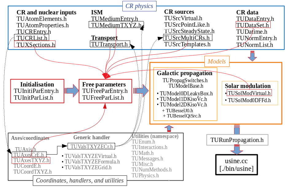
Figure 1: Organisation chart of usine classes.

The present version of the usine code was recently used to hint at the presence of a break in the diffusion coefficient from recent AMS-02 B/C data [27]. It was also used to rank the most important cross sections involved in Li, Be, B, C, and N fluxes for CR studies [28]. These two studies can be easily repeated and extended with the usine package as delivered, as illustrated in Sect. 6.

About previous unreleased versions

The first usine version was developed last century. With a growing interest for semi-analytical models, especially in the context of dark matter indirect detection, a public release was planned in the early 00’s, but was delayed for all these years: the first unreleased usine version (in C) was used to implement for the first time automated scan of the propagation parameter space [44, 45] and to study the impact of the local under-density on radioactive cosmic-rays [17]; the second unreleased version (in C/C++, interfaced with root cern) included anti-protons and anti-deuterons [18, 19], and was also interfaced, for the first time in the field, with a Markov Chain Monte Carlo engine [51, 52, 53, 12] to extract probability density functions of the fit parameters.

3.1 Code structure

Figure 1 shows a sketch of USINE classes grouped by items, underlying the most relevant features of the code. A detailed description of class members and their role is provided in the header files (include/TU*.h):

CR physics

(blue box, top): classes for CR base ingredients, with CR charts, data, and cross-sections set from input files (see Sect. 4).

Coordinates, handlers, and utilities

(grey box, bottom): one of the most important class in usine is TUValsTXYZCrE.h, a handler for formulae (or values on a grid), dependent on generic CR, energy, and space-time coordinates. The dashed arrows indicate the classes involved and where TUValsTXYZCrE.h is used (for transport, ISM description, and source parameters).

Models

(orange box, right-hand side): dedicated classes for Galactic propagation and Solar modulation models.

Initialisation

(red box, left-hand side): class reading the parameter file (see Sect. 5) to set and initialise all classes for a run.

Free parameters

(red box, centre): class handling all fit-able parameters. Red arrows connecting red boxes highlight classes with free parameters (spatial coordinates, cross sections, ISM, transport, sources, Solar modulation), see Sect. 5.5 for the syntax.

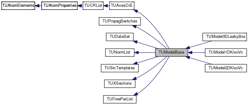
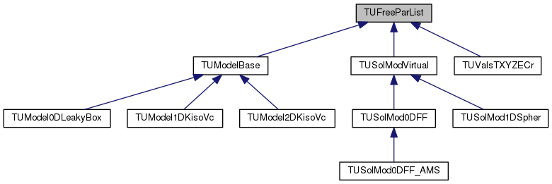
Figure 2: Inheritance diagram in usine for propagation model classes (top) and free parameters (bottom).

3.2 Inheritance diagrams

Two important classes in usine largely rely on inheritance and are shown in Fig. 2, as obtained running doxygen with graphviz enabled. First, all propagation models inherit from TUModelBase.h (top panel). The latter class gathers all ingredients shared by any model: it inherits from CR list (charts/properties) and energy ‘axis’, propagation switches (physics effects switched on or off), CR data, list of data on which to normalise primary fluxes, CR source templates (to be used as CR sources), cross-sections (inelastic, production, etc.), and a list of free parameters for the model; it also has, as members, transport parameters, ISM description, source description, and a list of all free parameters (model and ingredients). Second, free parameters for all relevant classes are stored in a TUFreeParList.h object. They are themselves collected in a global list of free parameters (bottom panel). This allows a very simple declaration of the parameters the user wishes to let free in a minimisation (see Sect. 5.5).

3.3 Focus on selected functions

I highlight in this section several important general-purpose functions, i.e. independent of the propagation model selected. All these functions belong to one of the c++ class listed in Fig. 1, and their identifiers are thus class::function.

Energy losses: TUInteractions::DEdtIonCoulomb()

Function to calculate Coulomb and ionisation losses in the ISM.

Secondaries: TUXSections::SecondaryProduction()

Integrates on all incoming projectile ($P$) energies, $E_{k/n}^{\rm in}$, the differential production cross sections of $F$ at $E_{k/n}^{\rm out}$:

$$\!\!\!\!\!\frac{dQ_{\rm sec}^{P\rightarrow F}}{dE_{k/n}^{\rm out}}(E_{k/n}^{\rm out})\!\! = \!\!\int_{0}^{\infty}dE_{k/n}^{\rm in}\;\frac{dN^{P}}{dE_{k/n}^{\rm in}}(E_{k/n}^{\rm in})$$

$$\times \!\!n_{\rm ISM}\times v^{\rm in}\times A_{F}\times\frac{d\sigma^{P+{\rm ISM}\rightarrow F}}{dE_{\rm tot}^{\rm out}}.$$

The extra factor $A_{F}$ originates from the conversion from differential kinetic energy per nucleon to differential total energy, which is the format of production cross sections files (see Sect. 4.4).

Tertiaries: TUXSections::TertiaryProduction()

$$\!\!\!\!\!\frac{dQ_{\rm ter}^{P}}{dE_{k/n}^{\rm out}}(E_{k/n}^{\rm out})\!\!\! = \!\!\!\int_{E_{k/n}^{\rm out}}^{\infty}\frac{dN^{P}}{dE_{k/n}^{\rm in}}(E_{k/n}^{\rm in})n_{\rm ISM}v^{\rm out}A_{P}\frac{d\sigma^{P+{\rm ISM}\rightarrow P}}{dE_{k}^{\rm out}}dE_{k/n}^{\rm in}$$ (3)

$$- \!\!\frac{dN^{P}}{dE_{k/n}^{\rm out}}(E_{k/n}^{\rm out})\times n_{\rm ISM}\times v^{\rm out}\times\sigma^{\rm ina}(E_{k/n}^{\rm out}),$$

with $\sigma^{\rm ina}$ the inelastic non-annihilating cross section. The extra factor $A_{P}$ originates from the conversion from total to kinetic energy per nucleon in the differential cross section. This equation is solved iteratively [e.g., 16], as implemented in each model class—for instance TUModel1DKisoVc::IterateTertiariesN0(). In usine, the tertiary contribution can be selected for any user-specified CR species (see Table 2), as long as the associated cross-section files exist. However, in practice, this contribution is only implemented where it matters, i.e. for anti-nuclei.

Solver for energy: TUModelBase::InvertForELossGain()

Fluxes are mostly power laws and kinetic energy per nucleon is approximately conserved in nuclear fragmentation reactions (straight-ahead approximation). This is the motivation to solve the second order differential equation in energy, Eq. (2), on a logarithmic scale in kinetic energy per nucleon. More specifically, for the model considered, one can always rewrite, after solving for the spatial coordinates (I omit the index $j$ and the $E_{k/n}$ dependence for readability):

$$n+A\frac{d}{d\ln E_{k/n}}\left(Bn-C\frac{dn}{d\ln E_{k/n}}\right)=S,$$

with $A,B,C$ and $S$ terms depending on the model parameters, energy losses and gains, and source and sink terms. Using a finite difference scheme with boundary conditions (see gENUM_BCTYPE in Table 1), this amounts to a tridiagonal matrix inversion that is inverted in TUNumMethods::SolveEq_1D2ndOrder_Explicit(). A detailed description of the chosen boundary conditions, their associated coefficients in the matrix, and the impact on the solution, as well as the stability of the numerical scheme, is provided in Sect. 3.1, App.C, and App D of [15] respectively.

Flux calculation: TUValsTXYZECr::OrphanVals()

The arguments of the function are quantity (e.g., B/C, O, etc.), energy type and grid (kEKN, kR…) on which to calculate quantity (see gENUM_ETYPE in Table 1), position in the model, and modulation model and level. The function proceeds as follow: (i) identify all isotopes in quantity, (ii) calculate IS flux for all isotopes at desired position, (iii) modulate all isotopes on same kinetic per nucleon grid, (iv) convert all results on desired grid and type (e.g., kR via a log-log interpolation), and finally (v) combine all the isotopic fluxes in the desired quantity.

$\chi^{2}$ calculation: TURunPropagation::Chi2_TOAFluxes()

The default configuration for the $\chi^{2}$ calculation is to loop over all time periods $t$ (corresponding to different modulation levels), all energy types $e$ selected of all quantities $q$ selected:

$$\chi^{2}_{\rm base}=\sum_{t,e,\,q}\left(\sum_{k=0}^{n(t,e,q)}\frac{({\rm data}_{k}-{\rm model}_{k})^{2}}{\sigma_{k}^{2}}\right),$$ (4)

with $n(t,e,q)$ the number of data and $\sigma_{k}$ the error on data. This calculation is modified for the following cases:

• Asymmetric error bars: I rely on the standard procedure, i.e. use in Eq. (4) the upper error $\sigma^{\rm up}$ (resp. $\sigma^{\rm lo}$) if the model is above the data (resp. below the data).

• Energy bin sizes: experiments provide the isotropic flux in the $i-$th energy bin, that is the number of events divided by the bin size. Rather than use the model value at the data mean energy, a more accurate calculation is to compare the data to

  $${\rm model}_{i}=\frac{\int_{E_{i}}^{E_{i+1}}{\rm model}(E)dE}{(E_{i+1}-E_{i})}.$$

  I assume that we have a power-law in the bin, $J=a\times E^{b}$, so that

  $${\rm model}_{i}\approx\frac{J_{i+1}\times E_{i+1}-J_{i}\times E_{i}}{(b+1)\times E_{i+1}-E_{i}},$$

  with $b=\ln(J_{i+1}/J_{i})/\ln(E_{i+1}/E_{i})$. This assumption can be refined by adding intermediate points (on which the power-law approximation is also assumed) : this is controlled by the parameter fNExtraInBinRange (see Table 5).

• Covariance: if a covariance matrix is provided (see Sect. 4.3) for a given $(t,e,q)$ dataset of $N_{E}$ energies, the corresponding term in Eq. (4) is replaced with:

  $$\chi^{2}_{\rm cov}=\sum_{\alpha}\sum_{i,j=0}^{n_{E},n_{E}}({\rm data}_{i}-{\rm model}_{i})({\cal C}^{\alpha})^{-1}_{ij}({\rm data}_{j}-{\rm model}_{j}),$$ (5)

  with ${\cal C}^{\alpha}_{ij}$ the covariance matrix provided by the user for the systematics $\alpha$ (several systematics with a different covariance may exist for a given set of data).

• Nuisance parameters: this version enables Gaussian-distributed nuisance parameters (see Sect. 5.5), each parameter ${\cal N}$ adding a contribution:

  $$\chi^{2}_{\rm nuis}=(\frac{{\cal N}-{\cal N}_{0}}{\sigma_{\cal N}})^{2}.$$ (6)

  Note that if a systematic error is set as nuisance parameter, it amounts to a model bias. For $N_{s}$ types of systematics set as nuisance for a given quantity, the model calculation reads

  $$\!\!\!{\rm model}_{k}\!\! = \!\!{\rm model}^{\rm true}_{k}\times{\rm bias}_{k}$$

  $$= \!\!{\rm model}^{\rm true}_{k}\times\Pi_{\alpha=0\dots N_{s}}(1+\nu^{\alpha}\times\sigma^{\alpha}_{k}),$$

  with $\nu^{\alpha}$ the error nuisance parameters for systematics $\alpha$ (centred on 0, variance 1), and $\sigma^{\alpha}_{k}$ the relative error for the energy $k$ read from the diagonal of the covariance matrix (we do not need the off-diagonal terms of the covariance matrix in that case, but I still use it as it was easier to implement it this way). In this very specific case, the systematics is not added in $\chi^{2}_{\rm cov}$, but only as a standard $\chi^{2}_{\rm nuis}$ (see above). The bias is accounted for and displayed in the result plots after minimisation (see Sect. 6.3).

3.4 Enumerators and keywords

The code contains many enumerators (enum key), most of them being relevant for developers only. The ones relevant for users are gathered in Table 1. They are used for parameter values in the initialisation file (Sect. 5) and/or as arguments of the executable ./bin/usine (Sect. 6). The complete list of enumerators is defined in include/TUEnum.h.

Table 1: Important usine enumerators and associated keywords.

Enumerators	Keywords	Description
gENUM_ETYPE⋆	kEKN	Kinetic E per nuc [GeV/n]​​​
	kR	Rigidity [GV]
	kETOT	Total energy [GeV]
	kEK	Kinetic energy [GeV]
gENUM_ERRTYPE§	kERRSTAT	Statistical only
	kERRSYST	Systematic only
	kERRTOT	Stat.+ syst. in quadrature​​​
	kERRCOV	Covariance matrix of errors​​​​
gENUM_FCNTYPE∘	kFORMULA	Formula (equation)
	kGRID	Values on a grid
gENUM_BCTYPE†	kNOCHANGE	Solution w/o = w/ E-losses​​​
	kD2NDLNEKN2_ZERO​​​	$\partial^{2}n/\partial(\ln E_{k/n})^{2}=0$
	kNOCURRENT	$j_{E}=0$
	kDFDP_ZERO	Flux derivative null
gENUM_PROPAG_MODEL​​​	kMODEL0DLEAKYBOX​​​​​	Leaky-box model
	kMODEL1DKISOVC​​​	1D diffusion model
	kMODEL2DKISOVC​​​	2D diffusion model
gENUM_SOLMOD_MODEL​​	kSOLMOD0DFF	Force-Field approximation​​​

^⋆ Energy type/unit for fits or displays.
^§ Data errors for fits or displays.
^∘ Parametrisation types for diffusion coefficient, source spectrum, etc.
^† Boundary condition at low or high energy end.

4 Input ASCII files (ingredients)

Galactic cosmic-ray propagation requires many inputs, which are handled by as many classes in usine, as shown in Fig. 1. Input files are ASCII files and default choices are given in inputs/. Users can feed to usine their own files and can locate them anywhere, as long as the path to the file is provided in the initialisation file. I give a short description below, and refer the reader to the online documentation for more details on the file format.

4.1 Atomic properties and CR charts

The file atomic_properties.dat gathers atomic properties for all possible CR elements. Some of these properties may be used for propagation, e.g. to account for an acceleration bias in source terms or for the calculation of electron attachment and stripping for electronic-capture (EC) decay.

The files crcharts_*.dat provide charts (mass, Z, A…) for CRs, and we only need to consider stable nuclei and unstable whose half-life is not too small compared to the propagation time. Ghost nuclei, unused for most usine runs, are also listed: they are short-lived isotopes whose decay chain leads to a stable (or long-lived) CR [40], and they enter the calculation of the cumulative cross-section into a given CR [e.g., 28].

4.2 Solar system (SS) abundances

Ideally, SS abundances should be used for comparison purpose after retro-propagating CR measurements back to the sources. However, propagation runs focusing on transport parameters use fixed values for the isotopic composition of elements, because CR isotopic data are scarce and only exist at low energy. The isotopic abundances of GCR sources can be initialised from solarsystem_abundances2003.dat, which gathers SS abundances for long-lived and stable isotopes and elements up to Uranium.

4.3 Cosmic-ray data and covariance matrix

The files crdata_*.dat contains list of data points (energy, value, date, name of experiment, etc.) directly retrieved from the cosmic-ray data base, CRDB [46]. One can also create her/his own data file from recent measurements or simulated data, and add it to the list of files to load in the initialisation file (Sect. 5). All energy types (gENUM_ETYPE) listed in Table 1 are enabled, so that CR data can be as a function of kinetic energy per nucleon, rigidity, etc.

The use of a covariance matrix of errors for minimisation is enabled in usine, and it requires one covariance matrix file per measurement (e.g., in directory CRDATA_COVARIANCE/). Actually, for past measurements, at best, only the overall uncertainties (statistical and systematics combined) were provided. In more recent data, at least statistical and systematic uncertainties are provided separately (format of data gathered in CRDB). Recent experiments (e.g., AMS02) go further and provide also systematics broken down in various contributions. However, this may not be sufficient for the model analysis of high-precision data, which may require the error correlations between different energies for all types of errors in the instrument, as encoded in the covariance matrix. The other option to deal with systematics uncertainties is via nuisance parameters (see Sect. 5.5), and it is not clear yet which is the best way to account for them.

4.4 Cross sections

The directories XS_NUCLEI/ and XS_ANTINUC/ provide energy-dependent cross sections for nuclei and anti-nuclei respectively, for both inelastic and production cross sections (straight-ahead or differential). For nuclei, production cross section files come in two flavours: those in which reactions for ‘ghosts’ (i.e. short-lived nuclei [40, 42]) are explicitly provided (XS_NUCLEI/GHOST_SEPARATELY/), and those with cumulative cross sections (XS_NUCLEI/). For instance, ${}^{10}{\rm B}$ has a single ghost nucleus, and its cumulative cross section from a CR species $X$ reads

$$\sigma^{\rm cumul}_{{\rm X}\rightarrow^{10}{\rm B}}=\sigma_{{\rm X}\rightarrow{\rm{}^{10}B}}+\sigma_{{\rm X}\rightarrow{\rm{}^{10}C}}\times{\cal B}r({\rm{}^{10}B}\rightarrow{\rm{}^{10}C})\,,$$

with ${\cal B}r({\rm{}^{10}B}\!\!\rightarrow\!\!{\rm{}^{10}C})=100\%$. Note that the heavier the species, the more ghost there are in general, though with smaller branching ratios. Whether files from XS_NUCLEI/ or XS_NUCLEI/GHOST_SEPARATELY/ are used, only stable and ‘long-lived’ ($\gtrsim$ kyr) species are propagated in usine; in the latter case, cumulative cross sections are re-calculated and weighted from the branching ratios of ghosts listed in crcharts_*.dat files (see online documentation). I recommend the user to rely on files with cumulative cross sections, unless separate cross sections are required for a specific use (e.g., [28]). Indeed, using cumulated cross sections ensures much faster propagation calculations for the same result. Speed and flexibility are also the reasons why I preferred pre-calculated cross sections over re-calculation for each run.

The format, content, and references for usine cross-section files (inelastic and production) are given in the online documentation. Some of the production cross sections were for instance obtained running WNEW [e.g., 64] and YIELDX [e.g., 62] codes with the usine or GALPROP [28] list of ghosts. For more details and references on the various models behind these cross sections, we refer the reader to [28] and [16, 20, 8, 18, 66, 37, 7] for nuclei and anti-nuclei respectively.

5 Initialisation file, models, and parameters

Any calculation with usine starts by loading an ASCII usine-formatted initialisation file. The file usage is flexible enough so that there is no need to recompile the code or go into it. The price to pay is a complicated syntax for the parameter values, which are described in a specific section of the code documentation. I only focus here on the structure and goal of the initialisation file.

The quantities initialised are the list of CRs to propagate and their parents (and associated charts), the energy ranges for the various species (nuclei, anti-nuclei, leptons), the cross sections and CR data to use, and then the propagation (ISM, source, transport) and solar modulation models. The parameters to fit, their range, and whether to use them as free or nuisance parameters is also completely handled by the same ASCII file.

5.1 Initialisation file syntax

Table 2: Example of base parameters from the initialisation file (Sect. 5). Only the last column (Value) should be edited.

Group    Subgroup	Parameter	Multi-entry?   Value
Base @ CRData	@ fCRData	@ M=1 @ $USINE/inputs/crdata….dat†
Base @ CRData	@ NormList	@ M=0 @ H,He:PAMELA$|$20$|$kEkn;C,N,O,F,Ne,Na,Mg,Al,Si:HEAO$|$10.6$|$kEkn
Base @ EnergyGrid	@ NBins	@ M=0 @ 129
Base @ EnergyGrid	@ NUC_EknRange	@ M=0 @ [5.e-2,5.e3]
Base @ EnergyGrid	@ ANTINUC_EknRange​​​	@ M=0 @ [5e-2,1.e2]
Base @ ListOfCRs	@ fAtomicProperties​​	@ M=0 @ $USINE/inputs/atomic_properties.dat†
Base @ ListOfCRs	@ fChartsForCRs	@ M=0 @ $USINE/inputs/crcharts….dat†
Base @ ListOfCRs	@ IsLoadGhosts	@ M=0 @ false
Base @ ListOfCRs	@ ListOfCRs	@ M=0 @ [2H-BAR,30Si]
Base @ ListOfCRs	@ ListOfParents	@ M=0 @ 2H-bar:1H-bar,1H,4He;1H-bar:1H,4He
Base @ ListOfCRs	@ PureSecondaries	@ M=0 @ Li,Be,B
Base @ ListOfCRs	@ SSRelativeAbund	@ M=0 @ $USINE/inputs/solarsystem_abundances2003.dat†
Base @ MediumCompo	@ Targets	@ M=0 @ H,He
Base @ XSections	@ Tertiaries	@ M=0 @ 1H-bar,2H-bar
Base @ XSections	@ fTotInelAnn	@ M=1 @ $USINE/inputs/XS_NUCLEI/sigInel….dat†
Base @ XSections	@ fProd	@ M=1 @ $USINE/inputs/XS_NUCLEI/sigProd….dat†
Base @ XSections	@ fProd	@ M=1 @ $USINE/inputs/XS_ANTINUC/dSdEProd….dat†
Base @ XSections	@ fTotInelNonAnn	@ M=1 @ $USINE/inputs/XS_ANTINUC/sigInelNONANN….dat†
Base @ XSections	@ fdSigdENAR	@ M=1 @ $USINE/inputs/XS_ANTINUC/dSdENAR….dat†

^† Any environment variable in file names (e.g., $USINE) is correctly interpreted.

An initialisation file consists of lines whose syntax is group @subgroup @parameter @M=…@value with many predefined keywords (see Tables 2 to 5). The rationale behind this choice is the following:

Group/subgroup/parameter

A parameter belongs to a subgroup, which itself belongs to a group. This allows to easily associate a parameter to a given physics ingredient and organise it in the initialisation file—the list of keywords is of course a matter of the developer’s taste, and for the user’s point of view, it is just what it is (not editable).

Multiple-entry parameter

Most of the time, parameters are single-valued ones (M=false or 0). However, CR data and cross-section files are enable for multiple-entries (M=true or 1), i.e. several files: in such case, the files are read sequentially, and the last read values always override previously read ones (if applies).

Value

This is editable by the user, to select files, parameter values, source spectrum energy dependences, fit parameters…each parameter value has a specific syntax.

We stress that the information (usage, specific syntax, example values) on any usine keyword can be accessed from the online documentation using the search box.

5.2 Base parameters

Base parameters consist in parameters that are required regardless of the propagation model used. Examples of base parameters are given in Table 2, and they correspond to:

• Base@CRData: selection of generic data sets and specific list of experiment and quantities (in the data sets) to renormalise the model to. For instance, the value H,He:PAMELA$|$20$|$kEkn;C,N,O,… in Table 2 means that usine will search for available H and He PAMELA data closest to 20 GeV/n (and a different set for C, N, O…), and use these points to renormalise the associated source terms keeping relative isotopic abundances fixed (unless these source terms are explicitly set as fit parameters).

• Base@EnergyGrid: different families of species (nuclei and anti-nuclei) are calculated on different kinetic energy per nucleon ranges, $[E_{\rm k/n}^{\rm min}-E_{\rm k/n}^{\rm max}]$, all on $N_{\rm bins}$ logarithmically-spaced bins:

  $$E_{\rm k/n}^{i}=E_{\rm k/n}^{\rm min}\times\Delta^{i},\quad{\rm with}\;\;\Delta=\left(\frac{E_{\rm k/n}^{\rm max}}{E_{\rm k/n}^{\rm min}}\right)^{1/(N_{\rm bins}-1)}.$$ (8)

  For anti-nuclei, integrations are involved (primary and tertiary source terms) and a doubling step integration is implemented to check the convergence on the available grid: the optimal number of bins to take is

  $$N_{\rm bins}=2^{j}+1.$$ (9)

  Note that E-range for nuclei should be larger than that for anti-nuclei, otherwise the high-energy flux of the latter is underestimated (protons at $E_{p}$ create $\bar{p}$ at $E_{\bar{p}}<E_{p}$).

• Base@ListOfCRs: (i) selection of atomic and nuclear charts files to select propagated CRs—value [2H-BAR,30Si] in Table 2 means all (anti-)nuclei from $\bar{d}$ to ³⁰Si; (ii) selection of the list of parents producing them—value1H-bar:1H,4He in Table 2 means that the parents for $\bar{p}$ are set to ¹H and ⁴He only; (iii) set the list of possible pure secondary species—Li,Be,B in Table 2 means that there is no source term for all isotopes of these elements.

• Base@MediumCompo: Choice of the ISM target elements for the propagation (e.g., H,He in Table 2). Any list is possible, without any change in the code (everything is allocated dynamically), but keep in mind that the production cross sections on these elements must then be provided.

• Base@XSections: Choice of the cross section files used for propagation. Internally, the code loops on all the files (all parameters are multi-entry ones). It fills and checks that all the cross sections associated to the list of CRs, parents (Base@ListOfCRs), and ISM targets (Base@MediumCompo) are found (inelastic and production cross-sections).

5.3 Model parameters

Table 3: Example of model parameters from the initialisation file (Sect. 5). Only the last column (Value) should be edited.

Group                     Subgroup	Parameter	Multi-entry?   Value
Model1DKisoVc​ @​ Geometry	@ ParNames	@ ​M=0​ @ L,h,rhole†
Model1DKisoVc​ @​ Geometry	@ ParUnits	@ ​M=0​ @ kpc,kpc,kpc†
Model1DKisoVc​ @​ Geometry	@ ParVals	@ ​M=0​ @ 8.,0.1,0.
Model1DKisoVc​ @​ Geometry	@ XAxis	@ ​M=0​ @ z:[0,L],10,LIN
Model1DKisoVc​ @​ Geometry	@ XSun	@ ​M=0​ @ 0.
Model1DKisoVc​ @​ ISM	@ Density	@ ​M=1​ @ HI:FORMULA$|$0.867
Model1DKisoVc​ @​ ISM	@ Density	@ ​M=1​ @ …
Model1DKisoVc​ @​ ISM	@ Te	@ ​M=0​ @ FORMULA$|$1.e4
Model1DKisoVc​ @​ SrcSteadyState​​​​​​​	@ Species​​​​​​​	@ ​M=1​ @ STD$|$ALL
Model1DKisoVc​ @​ SrcSteadyState​​​​​​​	@ SpectAbundInit​​​​​​​	@ ​M=1​ @ STD$|$kSSISOTFRAC,kSSISOTABUND,kFIPBIAS
Model1DKisoVc​ @​ SrcSteadyState​​​​​​​	@ SpectTempl​​​​​​​	@ ​M=1​ @ STD$|$POWERLAW$|$q
Model1DKisoVc​ @​ SrcSteadyState​​​​​​​	@ SpectValsPerCR​​​​​​​	@ ​M=1​ @ STD$|$q[PERCR:DEFAULT=1e-5];alpha[SHARED:2.];eta_s[SHARED:-1]​​​​​​​​​​​​​​
Model1DKisoVc​ @​ SrcSteadyState​​​​​​​	@ SpatialTempl​​​​​​​	@ ​M=1​ @ STD$|$-
Model1DKisoVc​ @​ SrcSteadyState​​​​​​​	@ SpatialValsPerCR​​​​​​​	@ ​M=1​ @ STD$|$-
Model1DKisoVc​ @​ Transport	@ ParNames	@ ​M=0​ @ Va,Vc,K0,delta,eta_t,Rb,Db,sb
Model1DKisoVc​ @​ Transport	@ ParUnits	@ ​M=0​ @ km/s,km/s,kpc^2/Myr,-,-,GV,-,-
Model1DKisoVc​ @​ Transport	@ ParVals	@ ​M=0​ @ 85,19,0.035,0.6,-0.1,125.,0.2,0.01
Model1DKisoVc​ @​ Transport	@ Wind	@ ​M=1​ @ W0:FORMULA$|$Vc†
Model1DKisoVc​ @​ Transport	@ VA	@ ​M=0​ @ FORMULA$|$Va†
Model1DKisoVc​ @​ Transport	@ K	@ ​M=1​ @ K00:FORMULA$|$beta^eta_t*K0*Rig^delta*(1+(Rig/Rb)^(Db/sb))^(-sb)​​​​​​​​​​​​​​
Model1DKisoVc @ Transport	@ Kpp	@ ​M=0​ @ FORMULA$|$(4./3.)*(Va*1.022712e-3*beta*Etot)^2/(K00*delta*…)​​​​​​​​​​​​​​
TemplSpectrum​ @​ POWERLAW	@ ParNames	@ ​M=0​ @ q,alpha,eta_s
TemplSpectrum​ @​ POWERLAW	@ ParUnits	@ ​M=0​ @ /(GeV/n/m3/Myr)†,-,-
TemplSpectrum​ @​ POWERLAW	@ Definition	@ ​M=0​ @ FORMULA$|$q*beta^(eta_s)*Rig^(-alpha)

$\dagger$ These values cannot be edited by the user, they are intrinsic properties of the model.

Each propagation model is associated with a keyword in the initialisation file, with 3 enabled models: Model0DLeakyBox [51], Model1DKisoVc [52], and Model2DKisoVc [44, 16, 52]. There are several mandatory subgroups for any galactic propagation models, and the syntax of their parameter values is illustrated in Table 3 for the 1D model, Model1DKisoVc. Note that geometry and ISM parameter names and units are uniquely associated to a given semi-analytical models and should never be modified.

• Model1DKisoVc@Geometry: Geometry, coordinate system, and Sun’s position for the model. Here, we have as parameters the half-halo size $L$ [kpc], the thin-disc half-size $h$ [kpc] (whose value should better not be changed), and a possible gas underdensity $rhole$ [kpc] (as described in [17, 52]). The 1D geometry is a linear grid in $z$ (first axis Xaxis) from 0 to $L$, and all geometry parameter names are enabled as free parameters.

• Model1DKisoVc@ISM: ISM parameters for the model. In all implemented models, the gas density is constant in the thin disc, so we do not need to declare specific free parameters for the ISM, and simply specify the ISM densities (HI, HII, H2, and heavier elements) and properties (e.g., $T^{\circ}$).

  Table 4: Example of model parameters from the initialisation file (Sect. 5). Only the last column (Value) should be edited.

  Group          Subgroup	Parameter	Multi-entry?   Value
  UsineRun@Calculation	@ BC_NUC_LE	@ M=0 @ kD2NDLNEKN2_ZERO
  UsineRun@Calculation	@ BC_NUC_HE	@ M=0 @ kNOCHANGE
  UsineRun@Calculation	@ EPS_ITERCONV	@ M=0 @ 1.e-6
  UsineRun@Calculation	@ EPS_INTEGR	@ M=0 @ 1.e-4
  UsineRun@Calculation	@ EPS_NORMDATA	@ M=0 @ 1.e-10
  UsineRun@Calculation	@ IsUseNormList	@ M=0 @ true
  UsineRun@Display	@ QtiesExpsEType	@ M=0 @ ALL
  UsineRun@Display	@ ErrType	@ M=0 @ kERRSTAT
  UsineRun@Display	@ FluxPowIndex	@ M=0 @ 2.8
  UsineRun@Models	@ Propagation	@ M=1 @ Model1DKisoVc
  UsineRun@Models	@ SolarModulation	@ M=1 @ SolMod0DFF
  UsineRun@OnOff	@ IsDecayBETA	@ M=0 @ true
  UsineRun@OnOff	@ IsDestruction	@ M=0 @ true
  UsineRun@OnOff	@ …	@ M=0 @ true

• Model1DKisoVc@SrcSteadyState: steady-state source description (CR content, spectra, and spatial distribution if needed) based on templates for the spectra and spatial distributions. For the model shown in Table 3, I defined a spectral template, TemplSpectrum@POWERLAW. The syntax for formulae is that of fparser, and in this example, the generic spectrum is:

  $${\rm Template}=q\times\beta^{eta\_s}\times R^{-alpha},$$ (10)

  where Rig, beta, gamma, p, Ekn, Ek, Etot are interpreted by usine as the CR rigidity, $\beta$, $\gamma$, etc. The template spectrum must always have a normalisation parameter (here $q$). The syntax to define the source spectrum for a specific list of species, is (i) to pick a name for this source (here STD); (ii) to specify which template it is based on and what is the normalisation parameter for this template (here POWERLAW with q); (iii) to specify how many free parameters will be created and their default value (all parameters of templates are enabled as free parameters). In this example, there is one free parameter per CR (q_1H, q_2H…q_30Si (internally created in usine), and universal free parameters eta_s and alpha. Note that for the 1D model, there is no source spatial dependence, so the associated parameter values are empty (-).

• Model1DKisoVc@Transport: usine enables the most generic description for the transport parameters, i.e. diffusion tensor $K_{ij}$, wind vector $W_{i}$, and reacceleration ($V_{a}$ and $K_{pp}$). For the isotropic and homogeneous diffusion, with constant wind perpendicular to the disc, the 1D and 2D models only allow for the components K00 and W0. As for the source spectrum, any function of (Rig, beta, gamma, p, Ekn, Ek, Etot) and user-defined names is enabled. In the example of Table 3,

  $$K_{00}=\beta^{\eta_{t}}K_{0}R^{\delta}\times\left[1+\left(\frac{R}{R_{b}}\right)^{\delta_{b}/s_{b}}\right]^{-s_{b}},$$ (11)

  corresponding to a broken power-law as used in [27]. Any of the transport parameters declared in Model1DKisoVc@Transport@ParNames can be used as a fit parameter.

5.4 Run parameters

These parameters are related to the selection of models (propagation and solar modulation), numerical precision for propagation calculation, and quantities to show in displays, as illustrated in Table 4.

• UsineRun@Calculation: this includes boundary conditions (BC) to use on both low and high-energy ends (see keywords in Table 1), the relative precision for integrations (e.g., secondary contribution from differential cross sections), iterative procedure (e.g, tertiaries for anti-nuclei), and normalisation to data.

• UsineRun@Display: this is purely for display purpose, to select which data will be shown with which errors. Use ALL to display all available data (see Sect. 4), or the syntax Qty1,Qty2:Exp1,Exp2:EType1;Qty3:Exp3:EType2. The error shown are selected from gENUM_ERRTYPE (see Table 1).

• UsineRun@Models: Propagation and Solar modulation models to use in run are selected from gENUM_PROPAG_MODEL and gENUM_SOLMOD_MODEL (see Table 1).

• UsineRun@OnOff: All physics effects—decay, inelastic interaction, energy losses, etc.—can be enabled or disabled in usine. This is especially useful for comparison purpose (see Sect. 6).

5.5 Fit parameters

Table 5: Example of fit parameters from the initialisation file (Sect. 5). Only the last column (Value) should be edited.

Group    Subgroup	Parameter	Multi-entry?   Value
UsineFit @ Config	@ Minimiser	@ M=0 @ Minuit2
UsineFit @ Config	@ Algorithm	@ M=0 @ combined
UsineFit @ Config	@ …
UsineFit @ TOAData	@ QtiesExpsEType	@ M=0 @ B/C:AMS:KR
UsineFit @ TOAData	@ ErrType	@ M=0 @ kERRCOV:$USINE/inputs/CRDATA_COVARIANCE/
UsineFit @ TOAData	@ EminData	@ M=0 @ 1.e-5
UsineFit @ TOAData	@ EmaxData	@ M=0 @ 1.e10
UsineFit @ TOAData	@ TStartData	@ M=0 @ 1950-01-01_00:00:00
UsineFit @ TOAData	@ TStopData	@ M=0 @ 2100-01-01_00:00:00
UsineFit @ FreePars	@ CRs	@ M=1 @ HalfLifeBETA_10Be:NUISANCE,LIN,[1.3,1.5],1.387,0.012
UsineFit @ FreePars	@ DataErr	@ M=1 @ SCALE_AMS02_201105201605__BC:NUISANCE,LIN,[-10,10],0.,1.
UsineFit @ FreePars	@ DataErr	@ M=1 @ UNF_AMS02_201105201605__BC:NUISANCE,LIN,[-10,10],0.,1.
UsineFit @ FreePars	@ Modulation	@ M=1 @ phi_AMS02_201105201605_:NUISANCE,LIN,[0.3,,1.1],0.73,0.2
UsineFit @ FreePars	@ SrcSteadyState	@ M=1 @ alpha:NUISANCE,LIN,[1.7.,2.5],2.3,0.1
UsineFit @ FreePars	@ Transport	@ M=1 @ eta_t:FIT,LIN,[-3,3],0.,0.1
UsineFit @ FreePars	@ Transport	@ M=1 @ delta:FIT,LIN,[0.2,0.9],0.6,0.02
UsineFit @ FreePars	@ XSection	@ M=1 @ EnhancePowHE_ALL:NUISANCE,LIN,[0.,2.],1.,1.
UsineFit @ FreePars	@ XSection	@ M=1 @ Norm_16O+H:NUISANCE,LIN,[0.7,1.3],1.,0.05
UsineFit @ FreePars	@ XSection	@ M=1 @ Norm_12C+H->11B:NUISANCE,LIN,[0.5,2.],1.,0.2
UsineFit @ FreePars	@ XSection	@ M=1 @ EAxisScale_12C+H->11B:NUISANCE,LIN,[0.5,1.5],1.,0.5

The implementation of minimisers in usine is based on the ROOT::Math::Minimizer wrapper. A minimisation run, based on $\chi^{2}$ (see Sect. 3), requires additional parameters, as illustrated in Table 5. The syntax of these parameters is detailed in the documentation, as it can be quite involved for free parameters.

• UsineFit@Config: selection of the minimiser configuration and its parameters. I use as default minuit2 (see online manual) and minos can be switched on to properly get uncertainties on the free parameters.

• UsineFit@TOAData: selection of CR data on which to fit, and whether to use covariance or not (if exists, see 4.3). For instance, in Table 5, I fit on B/C:AMS:KR, that is B/C$(R)$ from AMS data using a covariance matrix to be searched in the directory $USINE/inputs/CRDATA COVARIANCE, with no sub-selection on the energy and time ranges.

• UsineFit@FreePars: geometry, ISM, source, and transport parameters can all in principle be set as free parameters. In addition, modulation parameters and data error uncertainties (for all data periods used in the fit) can be added as nuisance parameters. The syntax of a fit or nuisance parameter is name:X,Y,[min,max],init,sigma. Use X = FIT to declare as a fit parameter or X = NUISANCE to assume a Gaussian distributed parameter ${\cal N}(\mu)=$ init, $\sigma=$ sigma, see Eq. (6); use Y = LIN or LOG to sample the parameter as name or $\log_{10}$(name). Note that values outside [min,max] are strongly penalised. In Table 5, I have for instance:

  • fit parameters: the universal slope alpha of the source spectrum (parameter SrcSteadyState), and the transport coefficients eta_t and delta (parameters Transport);

  • nuisance parameters: $t_{1/2}^{{}^{10}\rm Be}$ (parameter CRs), solar modulation level of the specified AMS data (parameter Modulation), inelastic and production cross-sections (parameters XSection), specific error systematics (parameters DataErr).

6 Executable, options, and outputs: run examples

The executable is a command-line with various options and arguments,

./bin/usine -option arg1 arg2...

where option redirects to specific runs (standard calculation, extra plots, minimisation), arg1 is always the initialisation file (see Sect. 5), and arg2 is generally an output directory.

Options

The five families of options are:

• ./bin/usine -l: local flux calculation showing only selected quantities;

• ./bin/usine -m: minimisation-related options, with -m1 to list fit-able parameters, and -m2 to perform minimisations;

• ./bin/usine -e: extra calculations and comparison plots via an interactive session;

• ./bin/usine -i: input files/properties to display CR data, cross sections, etc.;

• ./bin/usine -t: test functions for usine.

Each option comes with a mandatory list of arguments, which is self-explanatory for all the options above: the USAGE line gives the arguments, and the line EXAMPLE gives default values for all arguments (that can be run directly).

Initialisation files

Several initialisation files are shipped with this release: inputs/init.TEST.par is a test-only file, used to check the installation of usine classes and all models. We also provide one file per usine model: inputs/init.Model0D.par, inputs/init.Model1D.par, and inputs/init.Model2D.par for the LB, 1D, and 2D models respectively. Their settings allow to roughly match B/C AMS-02 data, and they can be used as a starting point for more elaborate analyses within these models. Note that with the choice of parameters, the 1D and 2D models differ by less than $0.1\%$, and the 1D and LB models by less than 2% over the AMS-02 B/C rigidity range. We also provide in the documentation additional configurations resulting for the full B/C analysis performed in [29].

Outputs

The outputs of any given run are ASCII files and images saved in the user-selected output directory (e.g., $USINE/output/ in the examples below). Available ASCII files are a log file of the run (usine.last_run.log), a backup of the initialisation file last run (usine.last_run.init.par), and many result files for propagated fluxes and ratios (local_fluxes*.out). Most usine options also produce ASCII files (description and timestamp in the header) associated to the shown plots (saved as .pdf and .png, and root cern macros .C files). Outputs related to the calculation of IS and TOA fluxes are similar for all models, only differing in their name. The spatial distribution of fluxes can be calculated for 1D and 2D models, but it is not an output yet in this release.

6.1 Local fluxes: ./bin/usine -l

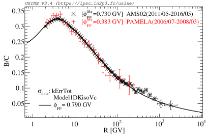
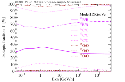
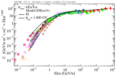
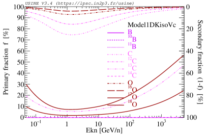
Figure 3: Plots from option -l. The left panels illustrate the display of a ratio and a flux in different energy unit ($R$ and $E_{k/n}$). For all user-selected CRs, usine also displays the energy-dependent fraction of all associated isotopes (top right), and the fraction of primary and secondary origin for each corresponding isotopes and elements (bottom right). See corresponding command line and full figure description in Sect. 6.1.

This option runs and calculates local fluxes, ratios, etc. for several modulation levels. Many plots and files are produced from the command line:
./bin/usine -l inputs/init.Model1D.par $USINE/output "B/C,B,C,O:KEKN:0.,1.;B/C:kR:0.79" 2.8 1 1 1

Figure 3 shows, from top to bottom, (i) B/C vs $R$ at selected modulation level along with selected CR data, (ii) C multiplied by $E_{k/n}^{2.8}$ vs $E_{k/n}$, (iii) isotopic fractions (form IS fluxes) vs $E_{k}{/n}$ for all isotopes involved in the selection, and (iv) primary (left axis) or secondary ($100-$primary, right axis) content of IS fluxes vs $E_{k/n}$ for all quantities involved in the selection.

6.2 Extra plots: ./bin/usine -e

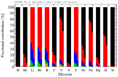
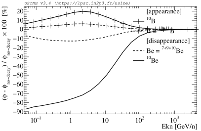
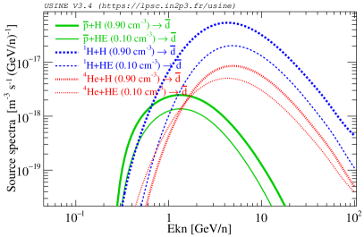
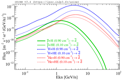
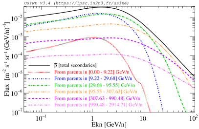
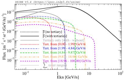
Figure 4: Sample of plots from option -e and sub-options D. Top panels: elemental fractional origins at three energies (left panel, see text for details), and impact of decay on propagated CR flux for an unstable species, its daughter, and associated elements (right panel). Middle panels: anti-deuteron contributions from CR projectiles and ISM targets separately at source (left panel, primary species folded to cross sections), or after propagation (right panel). Bottom panels: anti-proton spectrum broken-down in contributions from various energy ranges for parents (left-panel) or tertiaries (right panel). See corresponding command line and full figure description in Sect. 6.2.

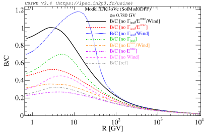
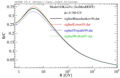
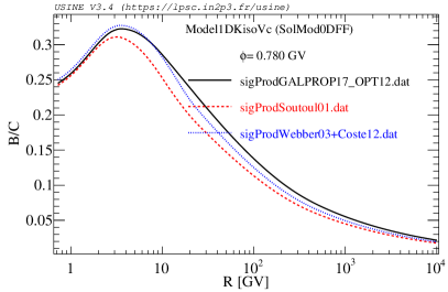
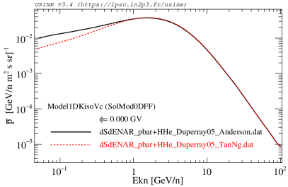
Figure 5: Plots from option -e and sub-options E. Calculations switching on and off several propagation effects for B/C (top left); effect of using different sets of inelastic (top right) and production (bottom left) cross sections on B/C; effects of using two different schemes for non-annihilating rescattering cross sections for anti-protons (bottom right). See corresponding command line and full figure description in Sect. 6.2.

An interactive session in which the user can loop on sub-options is started via the command line:
./bin/usine -e inputs/init.Model1D.par $USINE/output 1 1 1

Plots from sub-options -D

Figure 4 shows from top left to bottom right:

• D0: relative contributions per production process for elemental fluxes (isotopes not shown) at 1, 10, and 100 GeV/n: primary (black), secondary (1, 2, and $>2$ steps in red, blue, and green), radioactive (orange);

• D3: relative fraction of IS flux in excess or disappeared for $\beta$-radioactive isotope ¹⁰Be and its daughter ¹⁰B. The relative fraction for the element Be and B are also shown: the impact of decay is diluted by the other stable isotopes of the element);

• D5: separated source terms (before propagation) for CR+ISM reactions leading to $\bar{d}$;

• D6: separated $\bar{d}$ contributions (after propagation) for CR+ISM reactions;

• D7: secondary $\bar{p}$ contributions from different primary CR energy ranges;

• D8: tertiary $\bar{p}$ contribution. The black lines show the calculated flux without (dotted) and with (solid) the tertiary contribution: non-annihilating rescattering of $\bar{p}$ on the ISM deplete $\bar{p}$ at high energies and redistribute them at lower energies. The various colours show the contributions of various energy ranges.

Plots from sub-options -E

Figure 5 shows from top left to bottom right: From top left to bottom right:

• E2: comparison plot switching on/off physics effects during propagation (all other parameters being equal). In this example for B/C(R), the inelastic cross sections, reacceleration, and galactic wind have been switched-off in turns or together, compared to the reference (grey line).;

• E3: comparison plot using different inelastic cross-section parametrisations for nuclei;

• E4: comparison plot using different production cross-section parametrisations for nuclei;

• E8: comparison plot using different tertiary differential (redistribution) cross sections for $\bar{p}$.

6.3 Extra plots: ./bin/usine -m

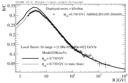
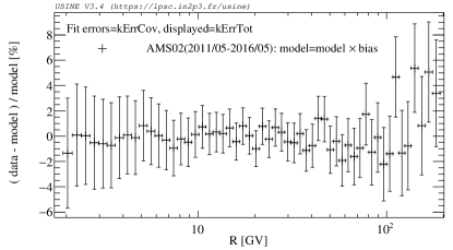
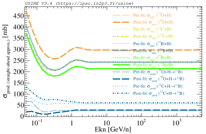
Figure 6: Plots from minimisation option -m2. In this example, based on inputs/init.TEST.par with modifications, the top panel illustrates the presence of a nuisance parameter on the data systematics (thin vs thick line), the middle panel shows residuals between data and best-fit model, and the bottom panel shows a comparison of pre- and post-fit cross-section nuisance parameters. See corresponding command line and full figure description in Sect. 6.3.

Minimisation runs with fit parameters, and possibly nuisance parameters and covariance matrix are performed with the command line:
./bin/usine -m2 inputs/init.TEST.par $USINE/output_fit 1 1 1

In addition to the information relative to the fit, several plots are displayed on screen, as illustrated in Fig. 6, from top to bottom:

• Best-fit obtained along with the data selected for display. If nuisance parameters are used for systematics errors of the fit data, both the model (thick line) and the biased model (thin line) are shown, with ${\rm bias}(R_{k})=\Pi_{l=0…n}(1+\nu_{l}\times\sigma_{l}(R_{k}))$.

• Residual between (biased)-model and data selected for the fit. The error bars correspond to the relative data errors.

• If specific cross sections are enabled as nuisance parameters (see Sect. 5.5), show the pre-fit (thin lines/small symbols) and post-fit cross sections (thick lines/large symbols) for comparison.

7 Conclusions

The usine code is a library for galactic cosmic-ray propagation, solving the diffusion equation for several semi-analytical models (LB, 1D-, and 2D-diffusion models). The code structure easily allows to add more complicated models, because many inputs, functions (to calculate primaries, secondaries, tertiaries…), and displays are of generic design and do not belong to any particular model.

A run configuration (ingredients, fixed and free parameters) is fully specified by a single ASCII file. To help navigate among the various inputs and keywords, an online documentation details all the files content and format, as well as the many keywords usage. Almost any model parameter (geometry, source, diffusion, ISM, Solar modulation level) can be set as a free parameter for minimisation studies. In addition, nuisance parameters on CR properties (e.g. decay time), cross sections (normalisation, high-energy dependence, etc.), and CR data (or correlation matrix) are enabled. These specificities were developed and taken advantage of to provide sound statistical analyses of recent high-precision AMS-02 data in [15, 29, 7].

Thanks to the speed of semi-analytical models, usine can also be used in an interactive mode, in which the calculation of IS fluxes is done once: a simple text interface allows users to loop on displayed fluxes and ratios at any modulation level. Extra plots for isotopic and primary fractions in CR fluxes, impact of decay, comparison of results using several cross-section files, etc. are also provided, and all associated data are saved in ASCII files. We stress that fluxes and ratios can be calculated for several energy units (rigidity, kinetic energy per nucleon, etc.), naturally matching units provided in different CR measurements. The latter can be extracted from CRDB [46], whose format is directly the one required by usine.

Many improvements are possible for a future release. My wish list would be the inclusion of electrons and positrons in 1D and 2D models following [6], the inclusion of dark matter contributions in 2D models (as was present in the second unreleased version of the code), the interface with MCMC engines, add splines as alternative to formulae in calculations, the proper inclusion of EC-decay CRs in propagation, 1D spherically symmetric Solar modulation model, and the extension of CR list and cross-section files for very heavy CRs ($Z>30$).

Appendix A Main features of usine v3.5

usine v3.5 was developed for the AMS-02 B/C and $\overline{p}$ analyses carried out in [15, 29, 7]. With respect to v3.4, it has more flexibility in the fit parameters and more plots for minimisation analyses. We list below the main improvements, and refer the reader to the version release notes for the full changes.

• Nuclear inelastic cross sections (inputs/XS_NUCLEI/) on He for the files sigInelBarashenkov94.dat, sigInelWellish97.dat, and sigInelWellish97.dat are now correctly based on [25]. I also removed sigInelLetaw83.dat because it is an older and less accurate version of sigInelWellish97.dat.

• New initialisation parameters for minimizer strategy and to save in ASCII files the covariance matrix of best-fit parameters (and Hessian).

• New prefixes to enable linear combination of cross section nuisance parameters (as described in [15]) and further flexibility in the selection of reactions.

• New keyword FIXED and unlimited range enabled for FIT and NUISANCE if minimiser allows.

• Source parameters (slope, normalisation, etc.) can now be SHARED (same for all CRs), PERCR (one per CR), PERZ (one per element), or LIST (any combination).

• Residuals and score plotted for minimisation, and plots of scans, profile likelihood, and contours enabled (with minuit) for FIT and NUISANCE parameters.

• For ./bin/usine -e runs, the detailed values of all the model free parameters are now shown in a display, and outputs results are now saved in ASCII files.

• New ./bin/usine -u to (i) show 1D and 2D probability density functions drawn from the covariance matrix of best-fit parameters, and (ii) show median and confidence levels on any quantity, as calculated from drawing samples of parameters from the best-fit values and covariance matrix, see Fig. 7. This option is only possible if the best-fit and covariance matrix of best-fit parameters were obtained previously with the -m2 option).

• Refactoring of several function in TURunPropagation to (i) separate calculation step to display step (new class TURunOutputs is used to store results and plot them); (ii) break-down $\chi^{2}$ function into more readable functions ($\chi^{2}$ from nuisance, $\chi^{2}$ from data, etc.).

• New ./bin/usine_pbar executable to propagate transport, source, and cross-section uncertainties to antiprotons. This was developed and used for the analysis in [7].

Figure 7: Plots from option -u. The top panel shows the probability density function of two parameters from the best-fit and covariance matrix of best-fit parameters of model big with AMS-02 B/C data [29], here for 10000 drawn values (option -u1). Bottom panel shows $1\sigma$ contours calculated from 100 drawn values of the same transport parameters for Li/C (option -u2).

References

- AMS Collaboration et al. [2016] AMS Collaboration, M. Aguilar, L. Ali Cavasonza, et al. Precision Measurement of the Boron to Carbon Flux Ratio in Cosmic Rays from 1.9 GV to 2.6 TV with the Alpha Magnetic Spectrometer on the International Space Station. Phys. Rev. Lett., 117(23):231102, December 2016. doi: 10.1103/PhysRevLett.117.231102.
- AMS Collaboration et al. [2017] AMS Collaboration, M. Aguilar, L. Ali Cavasonza, et al. Observation of the Identical Rigidity Dependence of He, C, and O Cosmic Rays at High Rigidities by the Alpha Magnetic Spectrometer on the International Space Station. Phys. Rev. Lett., 119(25):251101, December 2017. doi: 10.1103/PhysRevLett.119.251101.
- Berezinskii et al. [1990] V. S. Berezinskii, S. V. Bulanov, V. A. Dogiel, and V. S. Ptuskin. Astrophysics of cosmic rays. 1990.
- Bernard et al. [2012] G. Bernard, T. Delahaye, P. Salati, and R. Taillet. Variance of the Galactic nuclei cosmic ray flux. A&A, 544:A92, August 2012. doi: 10.1051/0004-6361/201219502.
- Binns et al. [2016] W. R. Binns, M. H. Israel, E. R. Christian, A. C. Cummings, G. A. de Nolfo, K. A. Lave, R. A. Leske, R. A. Mewaldt, E. C. Stone, T. T. von Rosenvinge, and M. E. Wiedenbeck. Observation of the 60Fe nucleosynthesis-clock isotope in galactic cosmic rays. Science, 352:677–680, May 2016. doi: 10.1126/science.aad6004.
- Boudaud et al. [2017] M. Boudaud, E. F. Bueno, S. Caroff, Y. Genolini, V. Poulin, V. Poireau, A. Putze, S. Rosier, P. Salati, and M. Vecchi. The pinching method for Galactic cosmic ray positrons: Implications in the light of precision measurements. A&A, 605:A17, September 2017. doi: 10.1051/0004-6361/201630321.
- Boudaud et al. [2019] Mathieu Boudaud, Yoann Génolini, Laurent Derome, Julien Lavalle, David Maurin, Pierre Salati, and Pasquale D. Serpico. AMS-02 antiprotons are consistent with a secondary astrophysical origin. arXiv e-prints, art. arXiv:1906.07119, Jun 2019.
- Bringmann and Salati [2007] T. Bringmann and P. Salati. Galactic antiproton spectrum at high energies: Background expectation versus exotic contributions. Phys. Rev. D, 75(8):083006, April 2007. doi: 10.1103/PhysRevD.75.083006.
- Brunetti and Codino [2000] M. T. Brunetti and A. Codino. Age of Cosmic-Ray Protons Computed Using Simple Configurations of the Galactic Magnetic Field. ApJ, 528:789–798, January 2000. doi: 10.1086/308186.
- Chandrasekhar [1943] S. Chandrasekhar. Stochastic Problems in Physics and Astronomy. Reviews of Modern Physics, 15:1–89, January 1943. doi: 10.1103/RevModPhys.15.1.
- Codino and Plouin [2006] A. Codino and F. Plouin. The Extension and Shape of the Collecting Zones of the Galactic Cosmic Rays from Helium to Iron. ApJ, 639:173–184, March 2006. doi: 10.1086/499201.
- Coste et al. [2012] B. Coste, L. Derome, D. Maurin, and A. Putze. Constraining Galactic cosmic-ray parameters with nuclei. A&A, 539:A88, March 2012. doi: 10.1051/0004-6361/201117927.
- Crank and Nicolson [1947] J. Crank and P. Nicolson. A practical method for numerical evaluation of solutions of partial differential equations of the heat-conduction type. Proceedings of the Cambridge Philosophical Society, 43:50, 1947. doi: 10.1017/S0305004100023197.
- Davis [1960] L. Davis, Jr. On the diffusion of cosmic rays in the galaxy. International Cosmic Ray Conference, 3:220, 1960.
- Derome et al. [2019] L. Derome, D. Maurin, P. Salati, M. Boudaud, Y. Génolini, and P. Kunzé. Fitting B/C cosmic-ray data in the AMS-02 era: a cookbook. arXiv e-prints, April 2019.
- Donato et al. [2001] F. Donato, D. Maurin, P. Salati, A. Barrau, G. Boudoul, and R. Taillet. Antiprotons from Spallations of Cosmic Rays on Interstellar Matter. ApJ, 563:172–184, December 2001. doi: 10.1086/323684.
- Donato et al. [2002] F. Donato, D. Maurin, and R. Taillet. beta -radioactive cosmic rays in a diffusion model: Test for a local bubble? A&A, 381:539–559, January 2002. doi: 10.1051/0004-6361:20011447.
- Donato et al. [2008] F. Donato, N. Fornengo, and D. Maurin. Antideuteron fluxes from dark matter annihilation in diffusion models. Phys. Rev. D, 78(4):043506, August 2008. doi: 10.1103/PhysRevD.78.043506.
- Donato et al. [2009] F. Donato, D. Maurin, P. Brun, T. Delahaye, and P. Salati. Constraints on WIMP Dark Matter from the High Energy PAMELA Data. Physical Review Letters, 102(7):071301, February 2009. doi: 10.1103/PhysRevLett.102.071301.
- Duperray et al. [2005] R. Duperray, B. Baret, D. Maurin, G. Boudoul, A. Barrau, L. Derome, K. Protasov, and M. Buénerd. Flux of light antimatter nuclei near Earth, induced by cosmic rays in the Galaxy and in the atmosphere. Phys. Rev. D, 71(8):083013, April 2005. doi: 10.1103/PhysRevD.71.083013.
- Evoli et al. [2008] C. Evoli, D. Gaggero, D. Grasso, and L. Maccione. Cosmic ray nuclei, antiprotons and gamma rays in the galaxy: a new diffusion model. J. Cosmology Astropart. Phys., 10:018, October 2008. doi: 10.1088/1475-7516/2008/10/018.
- Evoli et al. [2017] C. Evoli, D. Gaggero, A. Vittino, G. Di Bernardo, M. Di Mauro, A. Ligorini, P. Ullio, and D. Grasso. Cosmic-ray propagation with DRAGON2: I. numerical solver and astrophysical ingredients. J. Cosmology Astropart. Phys., 2:015, February 2017. doi: 10.1088/1475-7516/2017/02/015.
- Farahat [2010] A. Farahat. Markov stochastic technique to determine galactic cosmic ray sources distribution. Journal of Astrophysics and Astronomy, 31:81–88, June 2010. doi: 10.1007/s12036-010-0008-7.
- Farahat et al. [2008] A. Farahat, M. Zhang, H. Rassoul, and J. J. Connell. Cosmic Ray Transport and Production in the Galaxy: A Stochastic Propagation Simulation Approach. ApJ, 681:1334-1340, July 2008. doi: 10.1086/588374.
- Ferrando et al. [1988] P. Ferrando, W. R. Webber, P. Goret, J. C. Kish, D. A. Schrier, A. Soutoul, and O. Testard. Measurement of 12C, 16O, and 56Fe charge changing cross sections in helium at high energy, comparison with cross sections in hydrogen, and application to cosmic-ray propagation. Phys. Rev. C, 37:1490–1501, April 1988. doi: 10.1103/PhysRevC.37.1490.
- Genolini et al. [2017] Y. Genolini, P. Salati, P. D. Serpico, and R. Taillet. Stable laws and cosmic ray physics. A&A, 600:A68, April 2017. doi: 10.1051/0004-6361/201629903.
- Génolini et al. [2017] Y. Génolini, P. D. Serpico, M. Boudaud, S. Caroff, V. Poulin, L. Derome, J. Lavalle, D. Maurin, V. Poireau, S. Rosier, P. Salati, and M. Vecchi. Indications for a High-Rigidity Break in the Cosmic-Ray Diffusion Coefficient. Physical Review Letters, 119(24):241101, December 2017. doi: 10.1103/PhysRevLett.119.241101.
- Génolini et al. [2018] Y. Génolini, D. Maurin, I. V. Moskalenko, and M. Unger. Current status and desired precision of the isotopic production cross sections relevant to astrophysics of cosmic rays: Li, Be, B, C, and N. Phys. Rev. C, 98(3):034611, September 2018. doi: 10.1103/PhysRevC.98.034611.
- Genolini et al. [2019] Y. Genolini, M. Boudaud, P. Ivo Batista, S. Caroff, L. Derome, J. Lavalle, A. Marcowith, D. Maurin, V. Poireau, V. Poulin, S. Rosier, P. Salati, P. D. Serpico, and M. Vecchi. Cosmic-ray transport from AMS-02 B/C data: benchmark models and interpretation. arXiv: 1904.08917, April 2019.
- Ginzburg and Syrovatskii [1969] V. L. Ginzburg and S. I. Syrovatskii. The origin of cosmic rays. 1969.
- Jones [1970] F. C. Jones. Examination of the “Leakage-Lifetime” Approximation in Cosmic-Ray Diffusion. Phys. Rev. D, 2:2787–2802, December 1970. doi: 10.1103/PhysRevD.2.2787.
- Jones et al. [2001] F. C. Jones, A. Lukasiak, V. Ptuskin, and W. Webber. The Modified Weighted Slab Technique: Models and Results. ApJ, 547:264–271, January 2001. doi: 10.1086/318358.
- Kahneman [2011] Daniel Kahneman. Thinking, fast and slow. Farrar, Straus and Giroux, New York, 2011. ISBN 9780374275631 0374275637.
- Kissmann [2014] R. Kissmann. PICARD: A novel code for the Galactic Cosmic Ray propagation problem. Astroparticle Physics, 55:37–50, March 2014. doi: 10.1016/j.astropartphys.2014.02.002.
- Kopp et al. [2012] A. Kopp, I. Büsching, R. D. Strauss, and M. S. Potgieter. A stochastic differential equation code for multidimensional Fokker-Planck type problems. Computer Physics Communications, 183:530–542, March 2012. doi: 10.1016/j.cpc.2011.11.014.
- Kopp et al. [2014] A. Kopp, I. Büsching, M. S. Potgieter, and R. D. Strauss. A stochastic approach to Galactic proton propagation: Influence of the spiral arm structure. New A, 30:32–37, July 2014. doi: 10.1016/j.newast.2014.01.006.
- Korsmeier et al. [2018] Michael Korsmeier, Fiorenza Donato, and Mattia Di Mauro. Production cross sections of cosmic antiprotons in the light of new data from the NA61 and LHCb experiments. Phys. Rev. D, 97(10):103019, May 2018. doi: 10.1103/PhysRevD.97.103019.
- Lee [1979] M. A. Lee. A statistical theory of cosmic ray propagation from discrete galactic sources. ApJ, 229:424–431, April 1979. doi: 10.1086/156970.
- Lerche and Schlickeiser [1988] I. Lerche and R. Schlickeiser. On the energy spectrum of galactic primary cosmic rays - Results from the transport equation. Ap&SS, 145:319–354, June 1988. doi: 10.1007/BF00642108.
- Letaw et al. [1984] J. R. Letaw, R. Silberberg, and C. H. Tsao. Propagation of heavy cosmic-ray nuclei. ApJS, 56:369–391, November 1984. doi: 10.1086/190989.
- Lezniak [1979] J. A. Lezniak. The extension of the concept of the cosmic-ray path-length distribution to nonrelativistic energies. Ap&SS, 63:279–293, July 1979. doi: 10.1007/BF00638903.
- Maurin [2001] D. Maurin. Propagation des rayons cosmiques dans un modèle de diffusion : une nouvelle estimation des paramètres de diffusion et du flux d’antiprotons secondaires. PhD thesis, Université de Savoie, Février 2001. URL http://tel.archives-ouvertes.fr/docs/00/04/78/51/PDF/tel-00008773.pdf.
- Maurin and Taillet [2003] D. Maurin and R. Taillet. Spatial origin of Galactic cosmic rays in diffusion models. II. Exotic primary cosmic rays. A&A, 404:949–958, June 2003. doi: 10.1051/0004-6361:20030563.
- Maurin et al. [2001] D. Maurin, F. Donato, R. Taillet, and P. Salati. Cosmic Rays below Z=30 in a Diffusion Model: New Constraints on Propagation Parameters. ApJ, 555:585–596, July 2001. doi: 10.1086/321496.
- Maurin et al. [2002] D. Maurin, R. Taillet, and F. Donato. New results on source and diffusion spectral features of Galactic cosmic rays: I B/C ratio. A&A, 394:1039–1056, November 2002. doi: 10.1051/0004-6361:20021176.
- Maurin et al. [2014] D. Maurin, F. Melot, and R. Taillet. A database of charged cosmic rays. A&A, 569:A32, September 2014. doi: 10.1051/0004-6361/201321344.
- Merten et al. [2017] L. Merten, J. Becker Tjus, H. Fichtner, B. Eichmann, and G. Sigl. CRPropa 3.1 - a low energy extension based on stochastic differential equations. J. Cosmology Astropart. Phys., 6:046, June 2017. doi: 10.1088/1475-7516/2017/06/046.
- PAMELA Collaboration et al. [2014] PAMELA Collaboration, O. Adriani, G. C. Barbarino, et al. The PAMELA Mission: Heralding a new era in precision cosmic ray physics. Phys. Rep., 544:323–370, November 2014. doi: 10.1016/j.physrep.2014.06.003.
- Prishchep and Ptuskin [1975] V. L. Prishchep and V. S. Ptuskin. Decaying nuclei and the age of cosmic rays in the galaxy. Ap&SS, 32:265–271, February 1975. doi: 10.1007/BF00643139.
- Ptuskin et al. [1996] V. S. Ptuskin, F. C. Jones, and J. F. Ormes. On Using the Weighted Slab Approximation in Studying the Problem of Cosmic-Ray Transport. ApJ, 465:972, July 1996. doi: 10.1086/177482.
- Putze et al. [2009] A. Putze, L. Derome, D. Maurin, L. Perotto, and R. Taillet. A Markov Chain Monte Carlo technique to sample transport and source parameters of Galactic cosmic rays. I. Method and results for the Leaky-Box model. A&A, 497:991–1007, April 2009. doi: 10.1051/0004-6361/200810824.
- Putze et al. [2010] A. Putze, L. Derome, and D. Maurin. A Markov Chain Monte Carlo technique to sample transport and source parameters of Galactic cosmic rays. II. Results for the diffusion model combining B/C and radioactive nuclei. A&A, 516:A66, June 2010. doi: 10.1051/0004-6361/201014010.
- Putze et al. [2011] A. Putze, D. Maurin, and F. Donato. p, He, and C to Fe cosmic-ray primary fluxes in diffusion models. Source and transport signatures on fluxes and ratios. A&A, 526:A101, February 2011. doi: 10.1051/0004-6361/201016064.
- Schlickeiser [2002] R. Schlickeiser. Cosmic Ray Astrophysics. 2002.
- Soutoul et al. [1998] A. Soutoul, R. Legrain, A. Lukasiak, F. B. McDonald, and W. R. Webber. Evidence from Voyager and ISEE-3 spacecraft. Data for the decay of secondary K-electron capture isotopes during the propagation of cosmic rays in the Galaxy. A&A, 336:L61–L64, August 1998.
- Strauss and Effenberger [2017] R. D. T. Strauss and F. Effenberger. A Hitch-hiker’s Guide to Stochastic Differential Equations - Solution Methods for Energetic Particle Transport in Space Physics and Astrophysics. Space Sci. Rev., March 2017. doi: 10.1007/s11214-017-0351-y.
- Strong and Moskalenko [1998] A. W. Strong and I. V. Moskalenko. Propagation of Cosmic-Ray Nucleons in the Galaxy. ApJ, 509:212–228, December 1998. doi: 10.1086/306470.
- Strong et al. [2007] A. W. Strong, I. V. Moskalenko, and V. S. Ptuskin. Cosmic-Ray Propagation and Interactions in the Galaxy. Annual Review of Nuclear and Particle Science, 57:285–327, November 2007. doi: 10.1146/annurev.nucl.57.090506.123011.
- Taillet and Maurin [2003] R. Taillet and D. Maurin. Spatial origin of Galactic cosmic rays in diffusion models. I. Standard sources in the Galactic disk. A&A, 402:971–983, May 2003. doi: 10.1051/0004-6361:20030318.
- Taillet et al. [2004] R. Taillet, P. Salati, D. Maurin, E. Vangioni-Flam, and M. Cassé. The Effects of Discreteness of Galactic Cosmic-Ray Sources. ApJ, 609:173–185, July 2004. doi: 10.1086/421059.
- Tan and Ng [1983] L. C. Tan and L. K. Ng. Prediction of interstellar antiproton flux using a nonuniform galactic disk model. ApJ, 269:751–764, June 1983. doi: 10.1086/161084.
- Tsao et al. [1998] C. H. Tsao, R. Silberberg, and A. F. Barghouty. Partial Cross Sections of Nucleus-Nucleus Reactions. ApJ, 501:920–926, July 1998. doi: 10.1086/305863.
- Webber and Rockstroh [1997] W. R. Webber and J. M. Rockstroh. Monte Carlo calculations of cosmic ray electron and nuclei diffusion in the galaxy–a comparison of data and predictions. Advances in Space Research, 19:817–820, May 1997. doi: 10.1016/S0273-1177(96)00153-6.
- Webber et al. [1990] W. R. Webber, J. C. Kish, and D. A. Schrier. Formula for calculating partial cross sections for nuclear reactions of nuclei with E ~ 200 MeV/nucleon in hydrogen targets. Phys. Rev. C, 41:566–571, February 1990. doi: 10.1103/PhysRevC.41.566.
- Webber et al. [1992] W. R. Webber, M. A. Lee, and M. Gupta. Propagation of cosmic-ray nuclei in a diffusing galaxy with convective halo and thin matter disk. ApJ, 390:96–104, May 1992. doi: 10.1086/171262.
- Winkler [2017] Martin Wolfgang Winkler. Cosmic ray antiprotons at high energies. Journal of Cosmology and Astro-Particle Physics, 2017(2):048, Feb 2017. doi: 10.1088/1475-7516/2017/02/048.