Jointly learning relevant subgraph patterns and nonlinear models of their indicators

Abstract.

Classification and regression in which the inputs are graphs of arbitrary size and shape have been paid attention in various fields such as computational chemistry and bioinformatics. Subgraph indicators are often used as the most fundamental features, but the number of possible subgraph patterns are intractably large due to the combinatorial explosion. We propose a novel efficient algorithm to jointly learn relevant subgraph patterns and nonlinear models of their indicators. Previous methods for such joint learning of subgraph features and models are based on search for single best subgraph features with specific pruning and boosting procedures of adding their indicators one by one, which result in linear models of subgraph indicators. In contrast, the proposed approach is based on directly learning regression trees for graph inputs using a newly derived bound of the total sum of squares for data partitions by a given subgraph feature, and thus can learn nonlinear models through standard gradient boosting. An illustrative example we call the Graph-XOR problem to consider nonlinearity, numerical experiments with real datasets, and scalability comparisons to naïve approaches using explicit pattern enumeration are also presented.

1. Introduction

Graphs are fundamental data structures for representing combinatorial objects. However, precisely because of their combinatorial nature, it is usually difficult to understand the underlying trends in large datasets of graphs. The rapid increase in data in recent years also includes data represented as graphs, and thus supervised learning in which the inputs are graphs of arbitrary size and shape has gained considerable attention. This problem commonly arises in diverse fields such as cheminformatics (Kashima et al., 2003; Tsuda, 2007; Saigo et al., 2008; Saigo et al., 2009; Mahé and Vert, 2009; Vishwanathan et al., 2010; Shervashidze et al., 2011; Takigawa and Mamitsuka, 2013, 2017), and bioinformatics (Borgwardt et al., 2005; Karklin et al., 2005; Takigawa et al., 2011) as well as wide computer-science applications such as computer vision (Harchaoui and Bach, 2007; Nowozin et al., 2007; Barra and Biasotti, 2013; Bai et al., 2014), and natural language processing (Kudo et al., 2005).

The present paper investigates the supervised learning of a function $f:\mathcal{G}\to\mathcal{Y}$ from finite pairs of input graphs and output values, where $\mathcal{G}$ is a set of graphs and $\mathcal{Y}$ is a label space such as $\{-1,+1\}$ and $\mathbb{R}$. In general settings, the most fundamental and widely used features are indicators of subgraph patterns. Since the number of possible subgraph patterns are intractably large due to the combinatorial explosion, we need to use a heuristically limited class of subgraph patterns or to search for relevant patterns during the learning phase.

In addition to extensive studies on graph kernels (Kashima et al., 2003; Borgwardt et al., 2005; Harchaoui and Bach, 2007; Mahé and Vert, 2009; Vishwanathan et al., 2010; Shervashidze et al., 2011; Barra and Biasotti, 2013; Bai et al., 2014), joint learning of relevant subgraph patterns and classification/regression models by their indicators has also been developed (Kudo et al., 2005; Nowozin et al., 2007; Saigo et al., 2008; Saigo et al., 2009; Takigawa and Mamitsuka, 2017). This approach would not overlook any important features, but need some technical tricks to efficiently search for relevant subgraph patterns from combinatorially huge candidates. The previous methods use $\ell_{1}$ regularization for linear models of all possible subgraph indicators, and thus can select relevant subgraph patterns. In contrast, any practical graph kernels are based on all subgraphs in a predefined class, and do not try to select some relevant subsets of subgraph features. Note that the all-subgraphs kernel is known to be theoretically hard(Gärtner et al., 2003).

In the present paper, we investigate nonlinear models with all possible subgraph indicators. The following are the contributions of the present study:

• We present two lesser-recognized facts to make sure the difference between linear and nonlinear models of substructural indicators: (1) For a closely related problem of supervised learning from itemsets, the hypothesis space of the nonlinear model of all possible sub-itemset indicators is equivalent to that of the linear model; (2) Nevertheless, for the indicators of connected subgraphs, the hypothesis space of the nonlinear model is strictly larger than that of the linear model. (Section 4)

• We develop a novel efficient supervised learning algorithm for joint learning of all relevant subgraph features and a nonlinear models of their indicators. Unlike existing approaches based on $\ell_{1}$-regularized linear models, the proposed algorithm is based on gradient tree boosting with base regression trees selecting each splitter out of all subgraph indicators with an efficient pruning based on the new bound in Theorem 5.1. (Section 5)

• We empirically demonstrate that (i) for the Graph-XOR dataset, the proposed nonlinear method actually outperforms several linear methods, which implies the existence of problems requiring nonlinear hypotheses, (ii) For several real datasets, we also observe similar superiority of the nonlinear models for some datasets, while it also turns out that the performance of linear models is fairly comparable for some datasets. (Section 6)

1.1. Related Research and Our Motivation

Although not discussed explicitly, most previous studies (Kudo et al., 2005; Nowozin et al., 2007; Saigo et al., 2008; Saigo et al., 2009; Takigawa and Mamitsuka, 2017) yielded linear models with respect to subgraph indicators as Boolean variables. However, this would not be obvious at first glance because these studies were based on boosting such as Adaboost (Kudo et al., 2005) and LPBoost (Saigo et al., 2009), which are usually expected to produce nonlinear models. However, this is not the case because these studies used decision stumps with respect to a single subgraph feature as base learners.

The research of the present paper starts with our observation that replacing the decision stumps in these existing methods with decision trees is far from straightforward. This is because the previous methods are based on efficient pruning with specifically derived bounds to find a single best subgraph pattern, and use the indicator as a base learner at each iteration.

One naïve method to obtain nonlinear models of subgraph indicators is to enumerate some candidate subgraphs from training graphs, explicitly construct 0-1 indicator-feature vectors of test graphs by solving subgraph-isomorphism directly, and apply a general nonlinear supervised learning to those feature vectors. The performance with all small-size subgraphs occurred in the given graphs is known to be comparable for cheminformatics datasets(Wale et al., 2008). However these approaches would not scale well as we see later in Section 6.3. Another good known heuristic idea is to use $r$-neighborhood subgraphs with radius $r$ at each node as seen in ECFP(Rogers and Hahn, 2010) and graph convolutions(Kearnes et al., 2016; Gilmer et al., 2017). Unfortunately, the complete enumeration would not scale well either in this case, and usually requires some tricks such as feature hashing, feature folding, or feature embedding through neural nets, all of which are very interesting approaches but beyond the scope of this paper.

Note that it is not difficult to use the number of occurrences of subgraph $g$ in $G$ as features instead of just 0-1 subgraph indicators. Although not discussed herein, this case can be investigated as a weighted version of indicators, and similar properties would hold.

2. Preliminaries

2.1. Notations

Let $[n]$ be $\{1,2,\dots,n\}$, and let $\mathbb{I}(P)$ denote the indicator of $P$, i.e., $\mathbb{I}(P)=1$ if $P$ is true, else $0$. We denote as $G\sqsupseteq g$ the subgraph isomorphism that $G$ contains a subgraph that is isomorphic to $g$ and its negation as $G\not\sqsupseteq g$. Thus, a subgraph indicator $\mathbb{I}(G\sqsupseteq g)=1$ if $G\sqsupseteq g$, otherwise 0. We also denote the training set of input graphs $G_{i}\in\mathcal{G}$ and output responses $y_{i}\in\mathcal{Y}$ as

(1) $$\mathcal{D}=\{(G_{1},y_{1}),(G_{2},y_{2}),\dots,(G_{N},y_{N})\},$$

where $\mathcal{G}$ is a set of all finite-size, connected, discretely-labeled, undirected graphs. We denote $\mathcal{G}_{N}=\{G_{i}\mid i\in[N]\}$, and the set of all possible connected subgraphs as $\mathcal{S}_{N}=\bigcup_{G\in\mathcal{G}_{N}}\{g\mid G\sqsupseteq g\}$.

2.2. Search Space for Subgraphs

In supervised learning from graphs, we represent each input graph $G_{i}\in\mathcal{G}_{N}$ by the characteristic vector $(\mathbb{I}(G_{i}\sqsupseteq g)\mid g\in\mathcal{S})$ with a set $\mathcal{S}$ of relevant subgraph features. However, since $\mathcal{S}$ is not explicitly available when the learning phase starts, we need to jointly search and construct $\mathcal{S}$ during the learning process. In order to define an efficient search space for $\mathcal{S}_{N}$, i.e., any subgraphs occurring in $\mathcal{G}_{n}$, the techniques for frequent subgraph mining, which enumerates all subgraphs that appear in more than $m$ input graphs for a given $m$, are useful. Note that any subgraph feature $g\in\mathcal{S}_{N}$ can occur multiple times at multiple locations in a single graph, but $\mathbb{I}(G_{i}\sqsupseteq g)=1$.

In the present paper, we use the search space of the gSpan algorithm (Yan and Han, 2002), which performs a depth-first search on the tree-shaped search spaces on $\mathcal{S}_{N}$, referred to collectively as an enumeration tree, as shown in Figure 1. Each node of the enumeration tree holds a subgraph feature $g^{\prime}$ that extends the subgraph feature $g$ at the parent node by one edge, namely, $g^{\prime}\sqsupseteq g$.

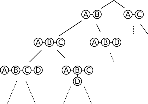
Figure 1. An enumeration tree

The following anti-monotone property of subgraph isomorphism over the enumeration tree on $\mathcal{S}_{N}$ can be used to derive the efficient search-space pruning of the gSpan algorithm:

(2) $$G_{i}\not\sqsupseteq g\Rightarrow G_{i}\not\sqsupseteq g^{\prime}\quad\text{for}\quad g^{\prime}\sqsupseteq g.$$

2.3. Gradient Tree Boosting

Gradient tree boosting (GTB) (Friedman, 2001; Mason et al., 2000) is a general algorithm for supervised learning to predict a response $y$ from a predictor $\bm{x}$. For a given hypothesis space $\mathcal{H}$, the goal is to minimize the empirical risk $L(f)=N^{-1}\sum_{i\in[N]}\ell(y_{i},f(\bm{x}_{i}))$ of $f\in\mathcal{H}$, which is the average of a loss function $\ell(y,f(\bm{x}))$ over the training data $\{(\bm{x}_{i},y_{i})\}_{i\in[N]}$.

GTB is an additive ensemble model of regression trees $T_{i}(\bm{x})$ of the form for fixed-stepsize cases:

$$f_{k}(\bm{x})=T_{0}+\eta\sum_{i\in[k]}T_{i}(\bm{x})$$

where $T_{0}$ is the mean of response variables in the training data, $\eta$ is the stepsize, and $T_{i}(\bm{x})$ is the $i$-th regression tree as a base learner. To fit the model to the training data, GTB performs the following gradient-descent-like iterations as a boosting procedure:

$$f_{0}(\bm{x})\leftarrow\arg\min_{c}\sum_{i\in[N]}\ell(y_{i},c),$$

$$\quad\text{and}\quad f_{k}(\bm{x})\leftarrow f_{k-1}(\bm{x})+\eta\,T_{k}(\bm{x}),$$

where $T_{k}(\bm{x})$ is a regression tree to best approximate the values of negative functional gradient $-\nabla_{f_{k-1}}L(f_{k-1})$ at $f_{k-1}$ obtained by fitting a regression tree to the data $\left\{\left(\bm{x}_{i},r_{i}\right)\right\}_{i\in[N]}$, where

$$r_{i}=-\left[\frac{\partial\,\ell(y_{i},f(\bm{x}_{i}))}{\partial f(\bm{x}_{i})}\right]_{f(\bm{x})=f_{k-1}(\bm{x}_{i})}$$

Our experiments focus on binary classification tasks with $y\in\{-1,+1\}$, and thus we use the logistic loss $\ell(y,\mu)=\log(1+\exp(-2y\mu))$. Note that even for classification, GTB must fit regression trees instead of classification trees in order to approximate real-valued functions.

The primary hyperparameters of GTB that we consider are the following three parameters: a max tree-depth $d$, a stepsize $\eta$, and the number of trees $k$.

2.4. Regression Trees

The internal regression-tree fitting is performed by the recursive partitioning below:

1. Each node in the regression tree receives a subset $\mathcal{D}^{\prime}\subseteq\mathcal{D}$ from the parent node.

2. If a terminal condition is satisfied, the node becomes a leaf decision node with a prediction value by the average of the response values in $\mathcal{D}^{\prime}$.

3. Otherwise, the node becomes an internal node that tries to find the best partition of $\mathcal{D}^{\prime}$ to $\mathcal{D}_{1}$ and $\mathcal{D}_{0}=\mathcal{D}^{\prime}\setminus\mathcal{D}_{1}$ that minimizes the total sum of squares of residual error $r$:

   $$\min_{\scalebox{1.0}{$\mathcal{D}_{1},\mathcal{D}_{0}$}}\bigl{[}\mathrm{TSS}(\mathcal{D}_{1})+\mathrm{TSS}(\mathcal{D}_{0})\bigr{]}.$$

   The subsets $\mathcal{D}_{1}$ and $\mathcal{D}_{0}$ are further sent to the child nodes, and Step (1) is then recursively applied to each subset at the child nodes.

$\mathrm{TSS}$ here is the total sum of squares of residual error $r$:

(3) $$\mathrm{TSS}(\mathcal{D})=\frac{1}{2}\sum_{i\in[N]}(r_{i}-\bar{r})^{2},\,\,\bar{r}=\frac{1}{N}\sum_{i\in[N]}r_{i}.$$

3. Problem Setting and Challenges

Our goal is learning a nonlinear model $f$ over all possible subgraph indicators $\mathbb{I}(G\sqsupseteq g)$ for $g\in\mathcal{S}_{N}$. As we will see in Section 4, arbitrary functions of subgraph indicators have a unique multi-linear polynomial form

$$f(G)=\sum_{S\subseteq\mathcal{S}_{N}}c_{S}\prod_{g\in S}\mathbb{I}(G\sqsupseteq g).$$

Input graphs are implicitly represented as a bag of subgraph features, and hence as feature vectors in which the elements are an intractably large number of binary variables of each subgraph indicator. The main challenge is how to learn the relevant features $g$ from such combinatorially large space $\mathcal{S}_{N}$ with also jointly learning the classifier $f$ over those features $\mathbb{I}(G\sqsupseteq g)$ for $g\in\mathcal{S}_{N}$. Other technical challenges are (1) feature vectors are binary valued and takes finite discrete values only at the vertices of a very high-dimensional Boolean hypercube; (2) feature vectors are strongly correlated due to subgraph isomorphism.

4. Pseudo-Boolean Functions of Substructural Indicators

We first investigate the difference between linear and nonlinear models. Any subgraph indicator $\mathbb{I}(G\sqsupseteq g)$ is a 0-1 Boolean variable, and thus the hypothesis space that we can consider with respect to these variables is a family of pseudo-Boolean functions, regardless of whether they are linear or nonlinear. A real-valued function $f:\{0,1\}^{d}\to\mathbb{R}$ on the Boolean hypercube $\{0,1\}^{d}$ is called pseudo-Boolean.

In this section, we explain the inequivalence of linear and nonlinear models of all possible subgraph indicators. Theorem 4.1, contrasting the difference from closely related problems for itemsets, suggests an advantage of the proposed nonlinear approach, and an illustrative example we call Graph-XOR indicating that linear models cannot learn is presented in Section 6.1.

Theorem 4.1.

(1) The hypothesis space of the nonlinear model of all possible sub-itemset indicators is equivalent to that of the linear model. (2) The hypothesis space of the nonlinear model of all possible connected subgraph indicators is strictly larger than that of the linear model.

This result is based on the following fundamental property of pseudo-Boolean functions.

Lemma 4.2.

(P.L. Hammer, 1963; Hammer and Rudeanu, 1968) Every pseudo-Boolean function $f:\{0,1\}^{d}\to\mathbb{R}$ has a unique multi-linear polynomial representation:

$$f(x_{1},\dots,x_{d})=\sum_{S\subseteq[d]}c_{S}\prod_{j\in S}x_{j},\quad x_{j}\in\{0,1\},\,\,c_{S}\in\mathbb{R}.$$

4.1. Sub-Itemset Indicators

Let $x_{j}\in\{0,1\}$ be a Boolean variable defined by $x_{j}=\mathbb{I}(j\in I)$ for an item $j\in[d]$ in a itemset $I\subseteq[d]$. Then we can see that linear and nonlinear models of sub-itemset indicators $\mathbb{I}(S\subseteq I),S\subseteq[d]$ are equivalent as a hypothesis space on itemsets. For any function $f:2^{[d]}\to\mathbb{R}$, we have

$$f(I) =\sum_{P\subseteq 2^{[d]}}c_{P}\prod_{S\in P}\mathbb{I}(S\subseteq I)=\sum_{U\in 2^{[d]}}c_{U}\mathbb{I}(U\subseteq I)$$

$$=\sum_{U\subseteq[d]}c_{U}\prod_{j\in U}\mathbb{I}(j\in I)$$

where $U=\bigcup_{S\in P}S$. Theorem 4.1 (1) follows from this simple fact. Note that including the negation terms, as in decision tree learning, does not change the hypothesis space because it can be represented as $\mathbb{I}(S\not\subseteq I)=1-\mathbb{I}(S\subseteq I)$.

4.2. Connected-Subgraph Indicators

As for subgraph indicators $\mathbb{I}(G\sqsupseteq g)$, the standard setting implicitly assumes that subgraph feature $g$ is a connected graph. This would be primarily because the complete search for subgraph patterns, including disconnected graphs, is practically impossible, given that even a set of all connected graphs $\mathcal{S}_{N}$ in $\mathcal{G}_{N}$, is already intractably huge in practice.

The difference between linear model $f_{L}(G)$ and nonlinear model $f_{NL}(G)$ is not constantly zero:

$$f_{L}(G) = c_{0}+\sum_{g\in\mathcal{S}_{N}}c_{g}\mathbb{I}(G\sqsupseteq g)$$

$$f_{NL}(G) = c_{0}+\sum_{g\in\mathcal{S}_{N}}c_{g}\mathbb{I}(G\sqsupseteq g)$$

$$+\sum_{S\subseteq\mathcal{S}_{N},|S|\geqslant 2}c_{S}\prod_{g\in S}\mathbb{I}(G\sqsupseteq g)$$

from which Theorem 4.1 (2) follows. This also implies that if we consider connected-subgraph-set indicators for the co-occurrence of several connected subgraphs, then the linear model is equivalent to the nonlinear model as a hypothesis space, and more importantly it is identical to $f_{NL}(G)$, which is the hypothesis space covered by the proposed algorithm in Section 5. Note that connected-subgraph-set indicators differ from the indicators of general subgraphs, including disconnected-subgraph-set indicators, because any subgraph feature $g\in\mathcal{S}$ can occur multiple times at different partially overlapped locations in a single graph. The hypothesis space by general subgraph indicators is beyond the scope of the present paper, and, in practice, the complete search for such indicators is computationally too challenging.

5. Proposed Method

In this section, we present a novel efficient method to produce a nonlinear prediction model based on gradient tree boosting with all possible subgraph indicators. Existing boosting-based methods (Kudo et al., 2005; Nowozin et al., 2007; Saigo et al., 2009) are based on simple but efficiently searchable base-learners of decision stumps (equivalent to subgraph indicators, as demonstrated previously) and construct an efficient pruning algorithm for this single best subgraph search at each iteration. In contrast, the proposed approach involves this subgraph search at finding an optimal split at each internal node of regression trees, while keeping the other outer loops the same as in GTB, as explained in Section 2.3. More specifically, we need to efficiently perform the following optimization over all possible subgraphs in $\mathcal{S}_{N}$:

(4) $$\min_{\scalebox{1.0}{$g\in\mathcal{S}_{N}$}}\Bigl{[}\mathrm{TSS}(\mathcal{D}_{1}(g))+\mathrm{TSS}(\mathcal{D}_{0}(g))\Bigr{]}$$

where $\mathrm{TSS}$ is the total sum of squares defined as (3), $\mathcal{D}_{1}(g)=\{(G_{i},r_{i})\in\mathcal{D}\mid G\sqsupseteq g\}$ and $\mathcal{D}_{0}(g)=\{(G_{i},r_{i})\in\mathcal{D}\mid G\not\sqsupseteq g\}$.

Here, $|\mathcal{S}_{N}|$ is too intractably huge to solve (4) by exhaustively testing subgraph $g\in\mathcal{S}_{N}$ in order, and thus we perform a branch and bound search over the enumerate tree on $\mathcal{S}_{N}$ with the following lower bound for the total sum of squares of expanded subgraphs:

Theorem 5.1.

Given $\mathcal{D}_{1}(g)$ and $\mathcal{D}_{0}(g)$, for any subgraph $g^{\prime}\sqsupseteq g$,

(5) $$\mathrm{TSS}(\mathcal{D}_{1}(g^{\prime}))+\mathrm{TSS}(\mathcal{D}_{0}(g^{\prime}))\geq\\ \min_{\scalebox{1.0}{$(\diamond,k)$}}\Big{[}\mathrm{TSS}(\mathcal{D}_{1}(g)\setminus S_{\diamond,k})+\mathrm{TSS}(\mathcal{D}_{0}(g)\cup S_{\diamond,k})\Big{]}$$

where $(\diamond,k)\in\{\leq,>\}\times\{2,\dots,|\mathcal{D}_{1}(g)-1|\}$, and $S_{\diamond,k}\subset\mathcal{D}_{1}(g)$, such that $S_{\leq,k}$ is a set of $k$ pair $(G_{i},r_{i})$ selected from $\mathcal{D}_{1}(g)$ in descending order of residual error $r_{i}$, and $S_{>,k}$ is that in increasing order. Note that $\setminus$, $\cup$ are set difference and set union respectively.

Proof.

The result follows from the property (2). See Appendix A for details. ∎

The entire procedure of the proposed algorithm is illustrated in Alg. 1 and 2. The novel algorithm for the optimal subgraph search of (4) using the bound (5) is described in detail in Alg. 3. In order to solve (4), the proposed algorithm uses a depth-first search on the enumerate tree over $\mathcal{S}_{N}$. The procedure at each subgraph $g$ is as follows:

1. Calculate the total sum of squares tss $\leftarrow\mathrm{TSS}(\mathcal{D}_{1}(g)+\mathcal{D}_{0}(g))$ of subgraph $g$.

2. Update min_tss by tss if min_tss $>$ tss.

3. Calculate bound (5) and if min_tss $<$ bound, then prune all child nodes of $g$.

Input: Training data $\mathcal{D}=\{(G_{1},y_{1}),(G_{2},y_{2}),\dots,(G_{N},y_{N})\}$, and stepsize $\eta$

Output: Prediction model $f:G\to\mathcal{Y}$

Function GradientTreeBoosting ($\mathcal{D}$)

       $f\leftarrow 1/N\sum_{i=1}^{N}y_{i}$ ;

       for $k=$1, 2, … do

             for $i\leftarrow 1$ to $N$ do

                   $r_{i}^{(k)}\leftarrow-\left[\frac{\partial\,\ell(y_{i},T(G_{i}))}{\partial T(G_{i})}\right]_{T(G)=T_{k-1}(G_{i})}$

             end for

            $T_{k}\leftarrow$ BuildRegressionTree ($\{(G_{i},r_{i}^{(k)})\mid i\in[N]\}$) ;

              $\triangleright$ Alg. 2

             $f\leftarrow f+\eta\,T_{k}$ ;

            

       end for

      return $f$

Alg. 1 Gradient Tree Boosting for Graphs

Input: Training data $\mathcal{D}=\{(G_{1},r_{1}),(G_{2},r_{2}),\dots,(G_{N},r_{N})\}$

Output: Regression tree $T$

Function BuildRegressionTree ($\mathcal{D}$)

       if the terminal condition is satisfied then

             make a leaf node in $T$ with the mean of $r_{i}$ ;

            

      else

             $g\leftarrow$ FindBestSplit ($\mathcal{D}$) ;

              $\triangleright$ Alg. 3

             make an internal node $v$ in $T$ with $g$ ;

             the left child of $v$ $\leftarrow$ BuildRegressionTree ($\mathcal{D}_{1}(g)$) ;

             the right child of $v$ $\leftarrow$ BuildRegressionTree ($\mathcal{D}_{0}(g)$) ;

            

       end if

      return T

Alg. 2 Regression Tree Learning for Graphs

Input: Training data $\mathcal{D}=\{(G_{1},r_{1}),(G_{2},r_{2}),\dots,(G_{N},r_{N})\}$

Output: Minimizer subgraph $g^{*}$ of (4)

Function FindBestSplit ($\mathcal{D}$)

       repeat

             $g$ $\leftarrow$ the next node of the enumeration tree by DFS ;

             tss $\leftarrow\mathrm{TSS}(\mathcal{D}_{1}(g))+\mathrm{TSS}(\mathcal{D}_{0}(g))$ ;

             if tss $<\textnormal{{min\_tss}}$ then

                   min_tss $\leftarrow$ tss ;

                   $g^{*}$ $\leftarrow$ $g$ ;

                  

             end if

            $\textnormal{{bound}}\leftarrow$ $\min_{(\diamond,k)}[\mathrm{TSS}(\mathcal{D}_{1}(g)\setminus S_{\diamond,k})+\mathrm{TSS}(\mathcal{D}_{0}(g)\cup S_{\diamond,k})]$ ;

              $\triangleright$ Theorem 5.1

             if min_tss $<\textnormal{{bound}}$ then

                   prune all children of $g$ in the enumeration tree ;

                  

             end if

            

      until the enumeration tree search ends;

      return $g^{*}$ ;

      

Alg. 3 Optimal Subgraph Search for Best Split

In the entire procedure, the most time-consuming part is the subgraph search (Alg. 3), which is repeatedly called during the learning process. Hence, introducing memorization, whereby we store expensive calls and return the cached results when the same pattern occurs again, can considerably speed up the entire process. First, we can store the result of minimization $\min_{\scalebox{1.0}{$g\in\mathcal{S}_{N}$}}(\mathrm{TSS}(\mathcal{D}_{1}(g))+\mathrm{TSS}(\mathcal{D}_{0}(g)))$ for each already checked $g$ and $\mathcal{D}$. Second, the subgraph search can be entirely skipped until we need to check any subgraph that has not been checked in any previous iterations.

6. Numerical Experiments

6.1. The Graph-XOR Problem

The linear separability has long been discussed using the XOR (or parity in general) example, and we present the same key example for graphs, referred to as Graph-XOR, where linear models cannot learn the target rule even when noiseless examples are provided.

The Graph-XOR dataset includes 1,035 graphs of seven nodes and six edges, where 506 are positives with $y=+1$ and 529 negatives with $y=-1$. As illustrated in Figure 3, each graph is generated by connecting two subgraphs by one node \raisebox{-0.7pt}{\footnotesize{D}}⃝. The component subgraphs are selected from the 18 types shown in Figure 3, where all three-node path graphs with candidate nodes {\raisebox{-0.7pt}{\footnotesize{A}}⃝, \raisebox{-0.7pt}{\footnotesize{B}}⃝, \raisebox{-0.7pt}{\footnotesize{C}}⃝}, and are randomly classified into two groups. Note that $\raisebox{-0.7pt}{\footnotesize{A}}⃝\text{--}\raisebox{-0.7pt}{\footnotesize{B}}⃝\text{--}\raisebox{-0.7pt}{\footnotesize{C}}⃝$ is isomorphic to $\raisebox{-0.7pt}{\footnotesize{C}}⃝\text{--}\raisebox{-0.7pt}{\footnotesize{B}}⃝\text{--}\raisebox{-0.7pt}{\footnotesize{A}}⃝$ and this duplicate redundancy due to the graph isomorphism is removed. The response value $y$ of a graph is $-1$ if two subgraphs are selected from the same group, otherwise $+1$.

Table 2 shows the performance results for the Graph-XOR data by two-fold cross validations. We use the proposed nonlinear method and two linear methods, namely, the proposed algorithm with maximum tree-depth ($d$) $=1$, i.e., with decision stumps, and a state-of-the-art (but linear) method for graphs, gBoost (Saigo et al., 2009). The hyperparameter tuning is performed for the ranges described in Table 1, and the best parameters are also listed in Table 2. Figures 4 and 5 show the accuracy and loss changes for the test data with regard to the max tree depth ($d$) and the max subgraph size ($x$). Here “subgraph size” means the number of edges.

The results shown in Table 2 clearly demonstrate that the linear models, including our model with $d=1$, fail, but the nonlinear methods work well. This is also theoretically supported by Theorem 4.1. Figure 4 also shows that only the behavior of $d=1$ differ from those of the other depths. Moreover, note that this problem at least requires subgraph features of size 2 (i.e., two edges), but searching excessively large subgraphs results in overfitting, as we see for $x$ $\geqslant 4$ in Figure 5.

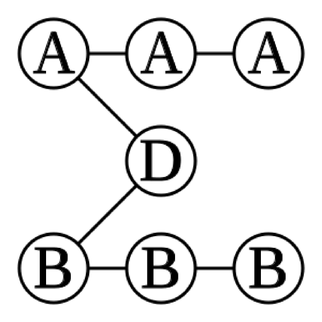
$y=+1$

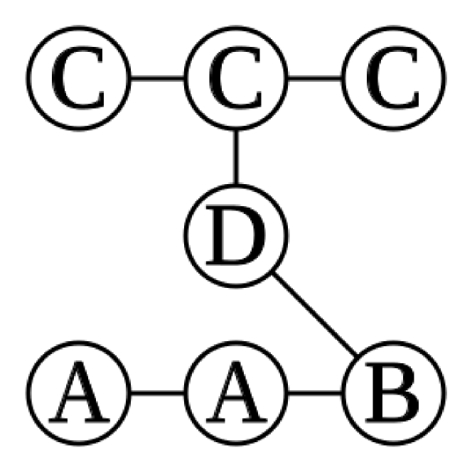
$y=+1$

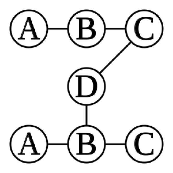
$y=-1$

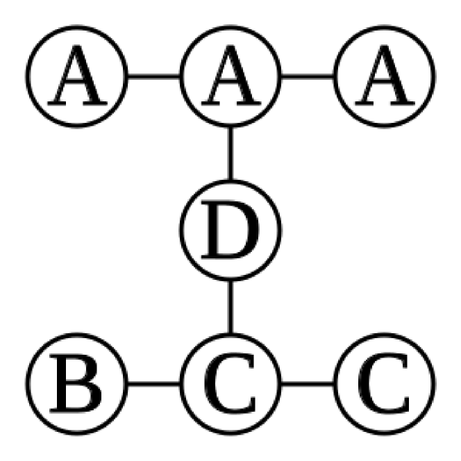
$y=-1$

Figure 2. Examples of the Graph-XOR data

Group 1	Group 2
\raisebox{-0.7pt}{\footnotesize{A}}⃝–\raisebox{-0.7pt}{\footnotesize{A}}⃝–\raisebox{-0.7pt}{\footnotesize{A}}⃝	\raisebox{-0.7pt}{\footnotesize{B}}⃝–\raisebox{-0.7pt}{\footnotesize{B}}⃝–\raisebox{-0.7pt}{\footnotesize{B}}⃝
\raisebox{-0.7pt}{\footnotesize{C}}⃝–\raisebox{-0.7pt}{\footnotesize{C}}⃝–\raisebox{-0.7pt}{\footnotesize{C}}⃝	\raisebox{-0.7pt}{\footnotesize{A}}⃝–\raisebox{-0.7pt}{\footnotesize{A}}⃝–\raisebox{-0.7pt}{\footnotesize{B}}⃝
\raisebox{-0.7pt}{\footnotesize{A}}⃝–\raisebox{-0.7pt}{\footnotesize{B}}⃝–\raisebox{-0.7pt}{\footnotesize{B}}⃝	\raisebox{-0.7pt}{\footnotesize{A}}⃝–\raisebox{-0.7pt}{\footnotesize{B}}⃝–\raisebox{-0.7pt}{\footnotesize{A}}⃝
\raisebox{-0.7pt}{\footnotesize{B}}⃝–\raisebox{-0.7pt}{\footnotesize{A}}⃝–\raisebox{-0.7pt}{\footnotesize{B}}⃝	\raisebox{-0.7pt}{\footnotesize{B}}⃝–\raisebox{-0.7pt}{\footnotesize{B}}⃝–\raisebox{-0.7pt}{\footnotesize{C}}⃝
\raisebox{-0.7pt}{\footnotesize{B}}⃝–\raisebox{-0.7pt}{\footnotesize{C}}⃝–\raisebox{-0.7pt}{\footnotesize{C}}⃝	\raisebox{-0.7pt}{\footnotesize{B}}⃝–\raisebox{-0.7pt}{\footnotesize{C}}⃝–\raisebox{-0.7pt}{\footnotesize{B}}⃝
\raisebox{-0.7pt}{\footnotesize{C}}⃝–\raisebox{-0.7pt}{\footnotesize{B}}⃝–\raisebox{-0.7pt}{\footnotesize{C}}⃝	\raisebox{-0.7pt}{\footnotesize{A}}⃝–\raisebox{-0.7pt}{\footnotesize{A}}⃝–\raisebox{-0.7pt}{\footnotesize{C}}⃝
\raisebox{-0.7pt}{\footnotesize{A}}⃝–\raisebox{-0.7pt}{\footnotesize{C}}⃝–\raisebox{-0.7pt}{\footnotesize{C}}⃝	\raisebox{-0.7pt}{\footnotesize{A}}⃝–\raisebox{-0.7pt}{\footnotesize{C}}⃝–\raisebox{-0.7pt}{\footnotesize{A}}⃝
\raisebox{-0.7pt}{\footnotesize{C}}⃝–\raisebox{-0.7pt}{\footnotesize{A}}⃝–\raisebox{-0.7pt}{\footnotesize{C}}⃝	\raisebox{-0.7pt}{\footnotesize{A}}⃝–\raisebox{-0.7pt}{\footnotesize{B}}⃝–\raisebox{-0.7pt}{\footnotesize{C}}⃝
\raisebox{-0.7pt}{\footnotesize{A}}⃝–\raisebox{-0.7pt}{\footnotesize{C}}⃝–\raisebox{-0.7pt}{\footnotesize{B}}⃝	\raisebox{-0.7pt}{\footnotesize{B}}⃝–\raisebox{-0.7pt}{\footnotesize{A}}⃝–\raisebox{-0.7pt}{\footnotesize{C}}⃝

Figure 3. Subgraph groups

Table 1. Hyperparameter settings for Graph-XOR

Common
max subgraph size (edges)		$x$	2, 3, 4, 5, $\infty$
Model specific
Proposed	max tree depth	$d$	1, 2, 3, 4, 5
	stepsize	$\eta$	1, 0.7, 0.4, 0.1, 0.01
	# trees	$k$	1-500
gBoost	regularization	$\nu$	0.6, 0.5, 0.4, 0.3, 0.2, 0.1, 0.01

Table 2. Prediction accuracy (%) for the Graph-XOR

Nonlinear models	Linear models
Proposed	Proposed ($d1$)	gBoost
100.0	64.3	70.0
$x2~{}d2~{}\eta 0.7~{}k221$	$x6~{}d1~{}\eta 0.7~{}k26$	$x6~{}\nu 0.01$

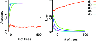
Figure 4. Test accuracy and loss with tree depth $d$

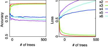
Figure 5. Test accuracy and loss with subgraph size $x$

6.2. QSAR with Molecular Graphs

We also evaluate the performance based on the most typical benchmark for graph classification on real datasets: the quantitative structure-activity relationship (QSAR) results with molecular graphs. We select four binary-classification datasets (CPDB, Mutag, NCI1, NCI47) in Table 3: two data (CPDB, Mutag) for mutagenicity tests and two data (NCI1, NCI47) for tumor growth inhibition tests from PubChem BioAssay. NCI1 and NCI47 are balanced by randomly sampling negatives of the same size as the positives in order to avoid imbalance difficulty in evaluation. All chemical structures are encoded as molecular graphs using RDKit, and some structures in the raw data are removed by chemical sanitization. We simply apply a node labeling by the RDKit default atom invariants (edges not labeled), i.e., atom type, # of non-H neighbors, # of Hs, charge, isotope, and inRing properties. These default atom invariants use connectivity information similar to that used for the well-known ECFP family of fingerprints(Rogers and Hahn, 2010). See (Kearnes et al., 2016) for more elaborate encodings.

Tables 5 and  6 show the performance results obtained by 10-fold cross validations using the same three methods used for the Graph-XOR cases with different hyperparameter settings in Table 4. We can observe that nonlinear methods often outperform the linear methods. At the same time, we can also observe, in some cases, that the linear methods work fairly well for the real datasets. The real datasets would not have explicit classification rules compared to noiseless problems such as the Graph-XOR cases. Thus, it is necessary to tolerate some noises and ambiguity. Although they may seem limited, linear hypothesis classes are known to be very powerful in such cases, because they are quite stable estimators and the input features can themselves include nonlinear features of data as implied in Theorem 4.1.

We also provide the normalized feature importance scores from GTB and the search space size in Figure 6 for the CPDB dataset. In Figure 6, searched corresponds to the searched subgraphs, and selected to the subgraph selected as internal nodes. This would also implies that (i) the proposed approach can provide information on selected relevant subgraph features and (ii) searches and uses only a portion of the entire search space.

Table 3. Dataset summary

Dataset	Graph- XOR	CPDB	Mutag	NCI1	NCI47
# data	1035	600	187	4252	4202
# nodes	7	13.7	17.9	26.3	26.3
# edges	6	14.2	19.7	28.4	28.4

        # of nodes and edges are average.

Table 4. Hyperparameter settings for the QSAR

Common
max subgraph size (# edges)		$x$	4, 6, 8
Model specific
Proposed	max tree depth	$d$	1, 3, 5
	stepsize	$\eta$	1.0, 0.7, 0.4, 0.1
	# trees	$k$	1-500
gBoost	regularization	$\nu$	0.6, 0.5, 0.4, 0.3, 0.2, 0.1, 0.01

Table 5. Prediction accuracy (%) for the QSAR

	CPDB		Mutag		NCI1		NCI47
	ACC	AUC	ACC	AUC	ACC	AUC	ACC	AUC
Nonlinear models
Proposed	79.3 ($\pm$4.8)	84.5 ($\pm$3.6)	87.8 ($\pm$6.6)	91.6 ($\pm$6.3)	84.7 ($\pm$1.7)	90.8 ($\pm$1.3)	84.5 ($\pm$1.7)	90.3 ($\pm$1.1)
Linear models
Proposed (d1)	79.3 ($\pm$4.4)	83.9 ($\pm$3.3)	87.8 ($\pm$6.6)	91.6 ($\pm$6.3)	83.1 ($\pm$1.6)	89.8 ($\pm$1.3)	82.8 ($\pm$1.4)	88.9 ($\pm$1.1)
gBoost	77.1 ($\pm$2.7)	73.6 ($\pm$4.9)	91.4 ($\pm$5.8)	93.9 ($\pm$5.0)	82.7 ($\pm$2.2)	83.9 ($\pm$2.2)	81.3 ($\pm$1.4)	81.8 ($\pm$2.6)
Reported values in literature
L1-LogReg (Takigawa and Mamitsuka, 2017)	78.3	-	-	-	-	-	-	-
MGK (Saigo et al., 2009)	76.5	75.6	80.8	90.1	-	-	-	-
freqSVM (Saigo et al., 2009)	77.8	84.5	80.8	90.6	-	-	-	-
gBoost (Saigo et al., 2009)	78.8	85.4	85.2	92.6	-	-	-	-
WL shortest path (Shervashidze et al., 2011)	-	-	83.7	-	84.5	-	-	-
Random walk (Shervashidze et al., 2011)	-	-	80.7	-	64.3	-	-	-
Shortest path (Shervashidze et al., 2011)	-	-	87.2	-	73.4	-	-	-

Table 6. Best hyperparameters

	CPDB	Mutag	NCI1	NCI47
Proposed	$x4~{}d5~{}\eta 0.1~{}k120$	$x4~{}d1~{}\eta 1~{}k22$	$x4~{}d5~{}\eta 0.1~{}k452$	$x4~{}d3~{}\eta 0.4~{}k308$
Proposed(d1)	$x8~{}d1~{}\eta 0.4~{}k128$	$x4~{}d1~{}\eta 1~{}k22$	$x4~{}d1~{}\eta 0.4~{}k499$	$x4~{}d1~{}\eta 0.4~{}k499$
gBoost	$x8~{}\nu 0.5$	$x7~{}\nu 0.1$	$x8~{}\nu 0.3$	$x8~{}\nu 0.4$

Figure 6. Feature importance and search space for CPDB

6.3. Scalability comparison to Naïve approach

As previously mentioned in Section 1.1, there exists a simple naïve two-step approach to obtain nonlinear models of subgraph indicators. Figure 7 shows the scalability of this “enumerate & learn” approach by first enumerating all small-size subgraphs and applying general supervised learning to their indicators. The values in the figure are the average values to process each fold in 10-fold cross validation on a single PC with Pentium G4560 3.50GHz and 8GB memory. We enumerate all subgraphs with limited subgraph size, and feed their indicator features to GradientBoostingClassifier with 100 trees (depth $\leqslant$ 5) of scikit-learn. The proposed method is also tested with the same setting (100 trees, d5). Since this case both use GTB and thus the performance is the same in principle up to implementation details (empirically both 0.75-0.77 for this setting), we focus on scalability comparisons using the fixed hyperparameters. Because the number of subgraph patterns to be enumerated increases exponentially, off-the-shelf packages such as scikit-learn cannot handle them at some point even when pattern enumeration can be done. In Figure 7, we can observe pattern enumeration can be done for max subgraph size = 1 to 12 (green line, left), but the 2nd scikit-learn step fails for max subgraph size $\geqslant 10$ (green line, right). In this CPDB examples, the numbers of subgraphs, i.e., the dimensions of feature vectors, were 66336.1, 145903.7, 275422.3, 512904.1, 874540.0 for max subgraph size = 8, 9, 10, 11, 12, respectively, and scikit-learn was only feasible for max subgraph size up to 9. Note that we also need to solve a large number of subgraph isomorphism known to be NP-complete.

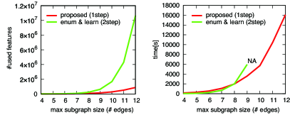
Figure 7. Scalability comparison to naïve approach

7. Conclusions

In summary, we investigated nonlinear models with all possible subgraph indicators and provide a novel efficient algorithm to learn from the nonlinear hypothesis space. We demonstrated that this hypothesis space is identical to the (pseudo-Boolean) functions of these subgraph indicators, which are, in general, strictly larger than those of the linear models. This is also empirically confirmed through our Graph-XOR example. Although most existing studies focus only on real datasets, this would also promote interest in whether graph-theoretic classification problems can be approximated in a supervised learning manner. At the same time, the experimental results of the present study also strongly suggest that we need a nonlinear hypothesis space for the QSAR problems based on some real datasets, which would also support a standard cheminformatics approach of applying nonlinear models, such as random forests and neural networks, to 0-1 feature vectors, referred to as molecular fingerprints, by the existence of substructural features.

Since research on classification and regression trees originates from the problem of automatic interaction detection (Morgan and Sonquist, 1963; Kass, 1975; Breiman et al., 1984), our approach can provide insights on the question whether such higher-order interactions between input features exist. In this sense, our methods and findings would also be informative to consider a recent hot topic of detecting such interactions in combinatorial data (Terada et al., 2013; Sugiyama et al., 2015; Nakagawa et al., 2015).

Appendix A Proof of Theorem 5.1

Proof.

Given $\mathcal{D}_{1}(g)$ and $\mathcal{D}_{0}(g)$,

bound $$=\min_{\scalebox{1.0}{$g^{\prime}$}}\bigl{[}\mathrm{TSS}(\mathcal{D}_{1}(g^{\prime}))+\mathrm{TSS}(\mathcal{D}_{0}(g^{\prime}))\bigr{]}$$

(6) $$=\min_{\scalebox{1.0}{$S\subset\mathcal{D}_{1}(g)$}}\bigl{[}\mathrm{TSS}(\mathcal{D}_{1}(g)\setminus S)+\mathrm{TSS}(\mathcal{D}_{0}(g)\cup S)\bigr{]}$$

(7) $$=\min_{\scalebox{1.0}{$(\diamond,k)$}}\Big{[}\mathrm{TSS}(\mathcal{D}_{1}(g)\setminus S_{\diamond,k})+\mathrm{TSS}(\mathcal{D}_{0}(g)\cup S_{\diamond,k})\Big{]}$$

where $(\diamond,k)\in\{\leq,>\}\times\{2,\dots,|\mathcal{D}_{1}(g)-1|\}$. From the anti-monotone property (2), we have $\mathcal{D}_{1}(g^{\prime})\subseteq\mathcal{D}_{1}(g)$ for $g^{\prime}\sqsupseteq g$ for the training set $\mathcal{D}$ from which the equation (6) directly follows. Thus, we show (7) in detail. For simplicity, let $A=,\{a_{1},\dots,a_{n}\mid a_{i}\in\mathbb{R}\}$ denote $\mathcal{D}_{1}(g)$, and $B=\{b_{1},\dots,b_{m}\mid b_{i}\in\mathbb{R}\}$ denote $\mathcal{D}_{0}(g)$. Then, the goal of (6) is to minimize the total sum of squares $\mathrm{TSS}(A\setminus S)+\mathrm{TSS}(B\cup S)$ by tweaking $S=\{s_{1},\dots,s_{k}\}\subset A$. Let $\bar{a}$, $\bar{a}_{-S}$, $\bar{b}$, and $\bar{b}_{+S}$ be the means of $A$, $A\setminus S$, $B$, and $B\cup S$, respectively. The key fact is that $\mathrm{TSS}(A\setminus S)+\mathrm{TSS}(B\cup S)$ can be regarded as a quadratic equation of $\sum_{i=1}^{k}s_{i}$ when the size of $S$ is fixed to $k$. More precisely,

$$\mathrm{TSS}(A\setminus S)+\mathrm{TSS}(B\cup S)$$

$$=\sum_{i\in[n]}(a_{i}-\bar{a}_{-S})^{2}-\sum_{i\in[k]}(s_{i}-\bar{a}_{-S})^{2}+\sum_{i\in[m]}(b_{i}-\bar{a}_{+S})^{2}+\sum_{i\in[k]}(s_{i}-\bar{a}_{+S})^{2}$$

$$=-\sum_{i\in[k]}(s_{i}-\bar{a})^{2}-\frac{\big{(}\sum_{i\in[k]}(s_{i}-\bar{a})\big{)}^{2}}{n-k}+\sum_{i\in[n]}(a_{i}-\bar{a})^{2}$$

$$\qquad+\sum_{i\in[k]}(s_{i}-\bar{b})^{2}-\frac{\big{(}\sum_{i\in[k]}(s_{i}-\bar{b})\big{)}^{2}}{m+k}+\sum_{i\in[m]}(b_{i}-\bar{b})^{2}$$

$$=-\left(\frac{1}{n-k}+\frac{1}{m+k}\right)\Big{(}\sum_{i\in[k]}s_{i}\Big{)}^{2}+\left(2\bar{a}\frac{n}{n-k}-2\bar{b}\frac{m}{m+k}\right)\sum_{i\in[k]}s_{i}$$

$$\qquad-\frac{nk}{n-k}\bar{a}^{2}+\frac{mk}{m+k}\bar{b}^{2}+\sum_{i\in[n]}(a_{i}-\bar{a})^{2}+\sum_{i\in[m]}(b_{i}-\bar{b})^{2}$$

Therefore, $\mathrm{TSS}(A\setminus S)+\mathrm{TSS}(B\cup S)$ is minimized when $\sum_{i=1}^{k}s_{i}$ is maximized or minimized. In other words, (6) becomes minimum when the mean of $S\subset\mathcal{D}_{1}(g)$ is maximized or minimized. ∎

References

- (1)
- Bai et al. (2014) Lu Bai, Luca Rossi, Horst Bunke, and Edwin R. Hancock. 2014. Attributed Graph Kernels Using the Jensen-Tsallis -Differences. In Proceedings of the 2014 European Conference on Machine Learning and Principles and Practice of Knowledge Discovery in Databases (ECML-PKDD 2014). Nancy, France, 99–114.
- Barra and Biasotti (2013) Vincent Barra and Silvia Biasotti. 2013. 3D shape retrieval using Kernels on Extended Reeb Graphs. Pattern Recognition 46, 11 (2013), 2985–2999.
- Borgwardt et al. (2005) Karsten M. Borgwardt, Cheng Soon Ong, Stefan Schönauer, S. V. N. Vishwanathan, Alex J. Smola, and Hans-Peter Kriegel. 2005. Protein Function Prediction via Graph Kernels. Bioinformatics 21, 1 (2005), i47–i56.
- Breiman et al. (1984) Leo Breiman, Jerome H. Friedman, Richard A. Olshen, and Charles. J. Stone. 1984. Classification and Regression Trees. Chapman and Hall/CRC, Belmont, California, U.S.A.
- Friedman (2001) Jerome H Friedman. 2001. Greedy Function Approximation: A Gradient Boosting Machine. Annals of statistics (2001), 1189–1232.
- Gärtner et al. (2003) Thomas Gärtner, Peter A. Flach, and Stefan Wrobel. 2003. On Graph Kernels: Hardness Results and Efficient Alternatives. In Proceedings of the 16th Annual Conference on Computational Learning Theory (COLT) and 7th Kernel Workshop. 129–143.
- Gilmer et al. (2017) Justin Gilmer, Samuel Schoenholz, Patrick F. Riley, Oriol Vinyals, and George Dahl. 2017. Neural Message Passing for Quantum Chemistry. In Proceedings of the 20th International Conference on Machine Learning (ICML). Washington, DC, USA.
- Hammer and Rudeanu (1968) Peter L Hammer and Sergiu Rudeanu. 1968. Boolean Methods in Operations Research and Related Areas. Springer.
- Harchaoui and Bach (2007) Zaïd Harchaoui and Francis Bach. 2007. Image Classification with Segmentation Graph Kernels. In Proceedings of the IEEE Computer Society Conference on Computer Vision and Pattern Recognition (CVPR). Minneapolis, Minnesota, USA, 1–8.
- Karklin et al. (2005) Yan Karklin, Richard F. Meraz, and Stephen R. Holbrook. 2005. Classification of non-coding RNA using graph representations of secondary structure. In Proceedings of the Pacific Symposium on Biocomputing (PSB). Hawaii, USA, 4–15.
- Kashima et al. (2003) Hisashi Kashima, Koji Tsuda, and Akihiro Inokuchi. 2003. Marginalized Kernels Between Labeled Graphs. In Proceedings of the 20th International Conference on Machine Learning (ICML). Washington, DC, USA, 321–328.
- Kass (1975) Gordon V. Kass. 1975. Significance Testing in Automatic Interaction Detection (A.I.D.). Journal of the Royal Statistical Society. Series C 24, 2 (1975), 178–189.
- Kearnes et al. (2016) Steven Kearnes, Kevin McCloskey, Marc Berndl, Vijay Pande, and Patrick Riley. 2016. Molecular graph convolutions: moving beyond fingerprints. Journal of Computer-Aided Molecular Design 30, 8 (01 Aug 2016), 595–608.
- Kudo et al. (2005) Taku Kudo, Eisaku Maeda, and Yuji Matsumoto. 2005. An Application of Boosting to Graph Classification. In Advances in Neural Information Processing Systems 17, Lawrence K. Saul, Yair Weiss, and Léon Bottou (Eds.). MIT Press, Cambridge, MA, 729–736.
- Mahé and Vert (2009) Pierre Mahé and Jean-Philippe Vert. 2009. Graph kernels based on tree patterns for molecules. Machine Learning 75, 1 (2009), 3–35.
- Mason et al. (2000) Llew Mason, Jonathan Baxter, Peter L Bartlett, and Marcus R Frean. 2000. Boosting Algorithms as Gradient Descent. In Advances in neural information processing systems. 512–518.
- Morgan and Sonquist (1963) James N. Morgan and John A. Sonquist. 1963. Problems in the analysis of survey data, and a proposal. J. Amer. Statist. Assoc. 58, 302 (1963), 415–434.
- Nakagawa et al. (2015) Kazuya Nakagawa, Shinya Suzumura, Masayuki Karasuyama, Koji Tsuda, and Ichiro Takeuchi. 2015. Safe Feature Pruning for Sparse High-Order Interaction Models. arXiv preprint arXiv:1506.08002 (2015).
- Nowozin et al. (2007) Sebastian Nowozin, Koji Tsuda, Takeaki Uno, Taku Kudo, and Gökhan Bakır. 2007. Weighted substructure mining for image analysis. In Proceedings of the IEEE Computer Society Conference on Computer Vision and Pattern Recognition (CVPR). Minneapolis, Minnesota, USA, 1–8.
- P.L. Hammer (1963) S. Rudeanu P.L. Hammer, I. Rosenberg. 1963. On the determination of the minima of pseudo-Boolean functions. Studii ¸si cercetari matematice 14 (1963), 359–364. in Romanian.
- Rogers and Hahn (2010) David Rogers and Mathew Hahn. 2010. Extended-connectivity fingerprints. Journal of Chemical Information and Modeling 50, 5 (2010), 742–754.
- Saigo et al. (2008) Hiroto Saigo, Nicole Krämer, and Koji Tsuda. 2008. Partial least squares regression for graph mining. In Proceeding of the 14th ACM SIGKDD international conference on Knowledge discovery and data mining. Las Vegas, Nevada, USA, 578–586.
- Saigo et al. (2009) Hiroto Saigo, Sebastian Nowozin, Tadashi Kadowaki, Taku Kudo, and Koji Tsuda. 2009. gBoost: a mathematical programming approach to graph classification and regression. Machine Learning 75 (2009), 69–89. Issue 1.
- Shervashidze et al. (2011) Nino Shervashidze, Pascal Schweitzer, Erik Jan van Leeuwen, Kurt Mehlhorn, and Karsten M. Borgwardt. 2011. Weisfeiler-Lehman Graph Kernels. Journal of Machine Learning Research 12, Sep (2011), 2539–2561.
- Sugiyama et al. (2015) Mahito Sugiyama, Felipe Llinares López, Niklas Kasenburg, and Karsten M Borgwardt. 2015. Significant Subgraph Mining with Multiple Testing Correction. In Proceedings of the 2015 SIAM International Conference on Data Mining. SIAM, 37–45.
- Takigawa and Mamitsuka (2013) Ichigaku Takigawa and Hiroshi Mamitsuka. 2013. Graph mining: procedure, application to drug discovery and recent advances. Drug Discovery Today 18, 1-2 (2013), 50–57.
- Takigawa and Mamitsuka (2017) Ichigaku Takigawa and Hiroshi Mamitsuka. 2017. Generalized Sparse Learning of Linear Models Over the Complete Subgraph Feature Set. IEEE Transactions on Pattern Analysis and Machine Intelligence 39, 3 (2017), 617–624.
- Takigawa et al. (2011) Ichigaku Takigawa, Koji Tsuda, and Hiroshi Mamitsuka. 2011. Mining Significant Substructure Pairs for Interpreting Polypharmacology in Drug-Target Network. PLoS ONE 6, 2 (2011), e16999. https://doi.org/10.1371/journal.pone.0016999
- Terada et al. (2013) Aika Terada, Mariko Okada-Hatakeyama, Koji Tsuda, and Jun Sese. 2013. Statistical significance of combinatorial regulations. Proceedings of the National Academy of Sciences 110, 32 (2013), 12996–13001.
- Tsuda (2007) Koji Tsuda. 2007. Entire regularization paths for graph data. In Proceedings of the 24th International Conference on Machine learning (ICML). Banff, Alberta, Canada, 919–926.
- Vishwanathan et al. (2010) S. V. N. Vishwanathan, Nicol N. Schraudolph, Risi Kondor, and Karsten M. Borgwardt. 2010. Graph Kernels. Journal of Machine Learning Research 11 (2010), 1201–1242.
- Wale et al. (2008) Nikil Wale, Ian A. Watson, and George Karypis. 2008. Comparison of descriptor spaces for chemical compound retrieval and classification. Knowledge and Information Systems 14, 3 (2008), 347–375.
- Yan and Han (2002) Xifeng Yan and Jiawei Han. 2002. gSpan: Graph-Based Substructure Pattern Mining. In Proceedings of the 2002 IEEE International Conference on Data Mining (ICDM). Washington, DC, USA, 721–724.