Scaling-Up Reasoning and Advanced Analytics on BigData

Abstract

BigDatalog is an extension of Datalog that achieves performance and scalability on both Apache Spark and multicore systems to the point that its graph analytics outperform those written in GraphX. Looking back, we see how this realizes the ambitious goal pursued by deductive database researchers beginning forty years ago: this is the goal of combining the rigor and power of logic in expressing queries and reasoning with the performance and scalability by which relational databases managed Big Data. This goal led to Datalog which is based on Horn Clauses like Prolog but employs implementation techniques, such as Semi-naïve Fixpoint and Magic Sets, that extend the bottom-up computation model of relational systems, and thus obtain the performance and scalability that relational systems had achieved, as far back as the 80s, using data-parallelization on shared-nothing architectures. But this goal proved difficult to achieve because of major issues at (i) the language level and (ii) at the system level. The paper describes how (i) was addressed by simple rules under which the fixpoint semantics extends to programs using count, sum and extrema in recursion, and (ii) was tamed by parallel compilation techniques that achieve scalability on multicore systems and Apache Spark. This paper is under consideration for acceptance in Theory and Practice of Logic Programming (TPLP).

1 Introduction

A growing body of research on scalable data analytics has brought a renaissance of interest in Datalog because of its ability to specify declaratively advanced data-intensive applications that execute efficiently over different systems and architectures, including massively parallel ones [Seo et al. (2013), Shkapsky et al. (2013), Yang and Zaniolo (2014), Aref et al. (2015), Wang et al. (2015), Yang et al. (2015), Shkapsky et al. (2016), Yang et al. (2017)]. The trends and developments that have led to this renaissance can be better appreciated if we contrast them with those that motivated the early research on Datalog back in the 80s. The most obvious difference is the great importance and pervasiveness of Big Data that, by enabling intelligent decision making and solving complex problems, is delivering major benefits to societies and economies. This is remarkably different from the early work on Datalog in the 80s, which was motivated by interest in expert system applications that then proved to be only of transient significance. The main objective of this paper is to present the significant technological advances that have made possible for Datalog to exploit the opportunities created by Big Data applications. One is the newly found ability to support a larger set of applications by extending the declarative framework of Horn clauses to include aggregates in recursive rules. The other is the ability of scaling up Datalog applications on Big Data by exploiting parallel systems featuring multicore and distributed architectures. We will next introduce and discuss the first topic, by summarizing the recent findings presented in [Zaniolo et al. (2017)] and then extending them with new examples of graph algorithms, and Knowledge Discovery and Data Mining (KDD) applications. The second topic is briefly discussed in this section; then it is revisited in Section 5 and fully discussed in Sections 6 and 7 on the basis of results and techniques from [Shkapsky et al. (2016)] and [Yang et al. (2017)].

A common trend in the new generation of Datalog systems is the usage of aggregates in recursion, since they enable the concise expression and efficient support of much more powerful algorithms than those expressible by programs that are stratified w.r.t. negation and aggregates [Seo et al. (2013), Shkapsky et al. (2013), Wang et al. (2015), Shkapsky et al. (2016)]. As discussed in more detail in the related work section, extending the declarative semantics of Datalog to allow aggregates in recursion represents a difficult problem that had seen much action in the early days of Datalog  [Kemp and Stuckey (1991), Greco et al. (1992), Ross and Sagiv (1992)]. Those approaches sought to achieve both (i) a formal declarative semantics for deterministic queries using the basic SQL aggregates, min, max, count and sum, in recursion and (ii) their efficient implementation by extending techniques of the early Datalog systems [Morris et al. (1986), Chimenti et al. (1987), Ramakrishnan et al. (1992), Vaghani et al. (1994), Arni et al. (2003)]. Unfortunately, as discussed in the Related Work section, some of those approaches had limited generality since they did not deal with all four basic aggregates, while the proposal presented in [Ross and Sagiv (1992)] that was covering all four basic aggregates using different lattices for different aggregates faced other limitations, including those pointed out by [Van Gelder (1993)] that are discussed in Section 8. These works were followed by more recent approaches that addressed the problem of using more powerful semantics, such as answer-set semantics, that require higher levels of computational complexity and thus are a better for higher-complexity problems than for the very efficient algorithms needed on Big Data [Simons et al. (2002), Pelov et al. (2007), Son and Pontelli (2007), Swift and Warren (2010), Faber et al. (2011), Gelfond and Zhang (2014)].

The recent explosion of work on Big Data has also produced a revival of interest in Datalog as a parallelizable language for expressing and supporting efficiently Big Data Analytics  [Seo et al. (2013), Shkapsky et al. (2013), Wang et al. (2015)]. As described from Section 5 onward, the projects discussed in those papers have demonstrated the ability of Datalog to provide scalable support for Big Data applications on both multicore and distributed systems. Most of the algorithms discussed in those papers are graph algorithms or other algorithms that use aggregates in recursion, whereby a full convergence of formal declarative semantics and amenability to efficient implementation becomes a critical objective. By supporting graph applications written in Datalog and compiled onto Apache Spark with better performance than the same applications written in GraphX (a Spark framework optimized for graph algorithms) and Scala (Spark’s native language), our BigDatalog system [Shkapsky et al. (2016)] proved that we have achieved this very difficult objective. Along with the post-MapReduce advances demonstrated by Apache Spark, this success was made possible by the theoretical developments presented in [Zaniolo et al. (2017)], where the concept of premappability ($\mathcal{}P$$\!reM$) was introduced for constraints using a unifying semantics that makes possible the use of the aggregates min, max, count and sum in recursive programs. Indeed, $\mathcal{}P$$\!reM$ of constraints provides a simple criterion that (i) the system optimizer can utilize to push constraints into recursion, and (ii) the user can utilize to write programs using aggregates in recursion, with the guarantee that they have indeed a formal fixpoint semantics. Along with its formal fixpoint semantics, this approach also extends the applicability of traditional Datalog optimization techniques, to programs that use aggregates in rules defining recursive predicates.

The rest of this paper is organized as follows. In the next section, we introduce the problem of supporting aggregates in recursion, then in Section 3 we present how such Datalog extension can be used in practice to implement efficient graph applications. We thus introduce in Section 4 even more advanced (KDD) analytics such as classification and regression. Sections 5, 6 and 7 introduce our BigDatalog and BigDatalog-MC systems that support scalable and efficient analytics through distributed and multicore architectures, respectively. Related work and conclusion presented in Sections 8 and 9 bring the paper to a closing.

2 Datalog Extensions: Min and Max in Recursive Rules

In this section, we first introduce some basics about Datalog before explaining its recent extensions. A Datalog program is formally represented as a finite set of rules. A Datalog rule, in turn, can be represented as $h\leftarrow b_{1},...,b_{n}$, where $h$ denotes the head of the rule and $b_{1},...,b_{n}$ represents the corresponding body. Technically, $h$ and each $b_{i}$ are literals assuming the form $p_{i}(t_{1},...,t_{j})$, where $p_{i}$ is a predicate and each $t_{i}$ can either be a constant or a variable. A rule with an empty body is called a fact. The comma separating literals in a body of the rule represents logical conjunction (AND). Throughout the paper we follow the convention that predicate and function names begin with lower case letters, and variable names begin with upper case letters.

A most significant advance in terms of language and expressive power offered by our systems [Shkapsky et al. (2016), Yang et al. (2017)] is that they provide a formal semantics and efficient implementation for recursive programs that use min, max, count and sum in recursion. We present here an informal summary of these advances for which [Zaniolo et al. (2017)] provides a formal in-depth coverage.

Consider for instance Example 1, where the goal $\mathtt{i}s\_min((X,Z),(Dxz))$ in $\mathtt{r}_{3}$ specifies that we want the min values of $\mathtt{D}xz$ for each unique pair of values $\mathtt{(}X,Z)$ in $\mathtt{d}path$ defined by rules $\mathtt{r}_{1}$ and $\mathtt{r}_{2}$.

Example 1 (Computing distances between node pairs, and finding their min)

$$\begin{array}[]{ll}&\mathtt{r}_{1}:dpath(X,Z,Dxz)~{}\mbox{<-}~{}\mathtt{d}arc(X,Z,Dxz).\\ &\mathtt{r}_{2}:dpath(X,Z,Dxz)~{}\mbox{<-}~{}\mathtt{d}path(X,Y,Dxy),darc(Y,Z,Dyz),\\ &\mathtt{~{}}~{}~{}~{}~{}~{}~{}~{}~{}~{}~{}~{}~{}~{}~{}~{}~{}~{}~{}~{}~{}~{}~{}~{}~{}~{}~{}~{}~{}~{}~{}~{}~{}~{}~{}~{}~{}~{}~{}~{}~{}~{}~{}~{}\mathtt{D}xz=Dxy+Dyz.\\ &\mathtt{r}_{3}:spath(X,Z,Dxz)~{}\mbox{<-}~{}\mathtt{d}path(X,Z,Dxz),is\_min((X,Z),(Dxz)).\\ \end{array}$$

Thus, the special notation $\mathtt{i}s\_min((X,Z),(Dxz))$ tells the compiler that $\mathtt{s}path(X,Z,Dxz)$ is a special predicate supported by a specialized implementation (the query and optimization techniques will be discussed in the following sections). Similar observations also hold for $\mathtt{i}s\_max$. However, the formal semantics of rules with extrema constructs is defined using standard (closed-world) negation, whereby the semantics of $\mathtt{r}_{3}$ is defined by the following two rules.

$$\begin{array}[]{ll}&\mathtt{s}path(X,Z,Dxz)~{}\mbox{<-}~{}\mathtt{d}path(X,Z,Dxz),\neg lesser(X,Z,Dxz).\\ &\mathtt{l}esser(X,Z,Dxz)~{}\mbox{<-}~{}\mathtt{d}path(X,Z,Dxz),dpath(X,Z,D1),D1<Dxz.\\ \end{array}$$

Expressing $\mathtt{i}s\_min$ via negation also reveals the non-monotonic nature of extrema constrains, whereby this program will be treated as a stratified program, with a "perfect model" semantics, realized by an iterated-fixpoint computation [Przymusinski (1988)]. In this computation, $\mathtt{d}path$ is assigned to a stratum lower than $\mathtt{s}path$ and thus the computation of $\mathtt{d}path$ must complete before the computation of $\mathtt{s}path$ via $\mathtt{i}s\_min$ in $\mathtt{r}_{3}$ can begin. This stratified computation can be very inefficient or even non-terminating when the original graph of Example 1 contains cycles. Thus, much research work was spent on solving this problem, before the simple solution described next emerged, and was used in and BigDatalogto support graph algorithms with superior performance [Shkapsky et al. (2016)]. This solution consists in taking the $\mathtt{i}s\_min$ constraint on $\mathtt{d}path$ in $\mathtt{r}_{3}$ and moving it to the rules $\mathtt{r}_{1}$ and $\mathtt{r}_{2}$ defining $\mathtt{d}path$, producing the rules in Example 2. This rewriting will be called a transfer of constraints.

Example 2 (Shortest Distances Between Node Pairs)

$$\begin{array}[]{ll}&\mathtt{r}^{\prime}_{1}:dpath(X,Z,Dxz)~{}\mbox{<-}~{}\mathtt{d}arc(X,Z,Dxz),is\_min((X,Z),(Dxz)).\\ &\mathtt{r}^{\prime}_{2}:dpath(X,Z,Dxz)~{}\mbox{<-}~{}\mathtt{d}path(X,Y,Dxy),darc(Y,Z,Dyz),\\ &\mathtt{~{}}~{}~{}~{}~{}~{}~{}~{}~{}~{}~{}~{}~{}~{}~{}~{}~{}~{}~{}~{}~{}~{}~{}~{}~{}~{}~{}~{}~{}~{}~{}~{}~{}~{}~{}~{}~{}~{}~{}~{}~{}~{}~{}~{}\mathtt{D}xz=Dxy+Dyz,is\_min((X,Z),(Dxz)).\\ &\mathtt{r}^{\prime}_{3}:spath(X,Z,Dxz)~{}\mbox{<-}~{}\mathtt{d}path(X,Z,Dxz).\\ \end{array}$$

While, at the syntactic level, this transfer of constraint is quite simple, at the semantic level, it raises the following two critical questions: (i) does the program in Example 2 have a formal semantics, notwithstanding the fact that it uses non-monotonic constructs in recursion, and (ii) is it equivalent to the original program, insofar as it produces the same answers for $\mathtt{s}path$? A positive formal answer to both questions was provided in [Zaniolo et al. (2017)] using the notion of premappability ($\mathcal{}P$$\!reM$) which is summarized next.

Premappability ($\mathcal{}P$$\!reM$) for Constraints.

Let $T$ denote the Immediate Consequence Operator (ICO) for the rules defining a recursive predicate. Since our rules are positive, the mapping defined by $T$ has a least-fixpoint in the lattice of set containment. Moreover the property that such least-fixpoint is equivalent to the fixpoint iteration $T^{\uparrow\omega}(\emptyset)$ allows us to turn this declarative semantics into a concrete one. Now let $\gamma$ be a constraint, such as an extrema constraint like min. We have the following important definition:

Definition 1

The constraint $\gamma$ is said to be $\mathcal{}P$$\!reM$ to $T$ when, for every interpretation $I$, we have that: $\gamma(T(I))=\gamma(T(\gamma(I)))$.

For convenience of notation, we will also denote by $T_{\gamma}$ the composition of the function $T$ with the function $\gamma$, i.e., $T_{\gamma}(I)=\gamma(T(I))$, which will be called the constrained immediate consequence operator for $T$ and the rules having $T$ as their ICO. Then, $\mathcal{}P$$\!reM$ holds whenever $T_{\gamma}(I)=T_{\gamma}(\gamma(I))$. We will next focus on cases of practical interest where the transfer of constraints under $\mathcal{}P$$\!reM$ produces optimized programs that are safe and terminating (even when the original programs do not terminate). Additionally, we prove that the transformation is indeed equivalence-preserving. Thus we focus on situations where $T_{\gamma}^{\uparrow n}(\emptyset)=T_{\gamma}^{\uparrow n+1}(\emptyset)$, i.e., the fixpoint iteration converges after a finite number of steps $n$. The rules defining a recursive predicate $p$ are those having as head $p$ or predicates that are mutually recursive with $p$. Then the following theorem was proven in  [Zaniolo et al. (2017)]:

Theorem 1

In a Datalog program, let $T$ be the ICO for the positive rules defining a recursive predicate. If the constraint $\gamma$ is $\mathcal{}P$$\!reM$ to $T$, and a fixpoint exists such that $T^{\uparrow n+1}(\emptyset)=T^{\uparrow n}(\emptyset)$ for some integer $n$, then $\gamma(T^{\uparrow\omega}(\emptyset))=T_{\gamma}^{\uparrow n}(\emptyset)$.

In [Zaniolo et al. (2017)] it was also shown that the fixpoint so derived is a minimal fixpoint for the program produced by the transfer of constraints. Thus if a constraint is $\mathcal{}P$$\!reM$ to the given recursive rules, its transfer produces an optimized program having a declarative semantics defined by the minimal fixpoint of its constrained ICO $(T_{\gamma})$ and operational semantics supported by a terminating fixpoint iteration, with all the theoretical and computational properties that follow from such semantics. For instance, $\mathcal{}P$$\!reM$ for extrema constraints holds for Example 1, and since directed arcs in our graph have non-negative lengths, we conclude that its optimized version in Example 2 terminates even if the original graph has cycles.

For most applications of practical interest, $\mathcal{}P$$\!reM$ is simple for users to program with, and for the system to support. For instance, to realize that $\mathcal{}P$$\!reM$ of min and max holds for the rules for our Example 1, the programmer will test $\mathcal{}P$$\!reM$ by asking how the mapping established by rules $\mathtt{r}^{\prime}_{1}$ and $\mathtt{r}^{\prime}_{2}$ in Example 2 changes if, in addition to the post-constraint $\mathtt{i}s\_min$ that applies to the cost arguments of the head of rules $\mathtt{r}^{\prime}_{1}$ and $\mathtt{r}^{\prime}_{2}$, we add the goal $\mathtt{i}s\_min$ in the body of our two rules to pre-constrain the values of the cost argument in every $\mathtt{d}path$ goal. Of course, $\mathcal{}P$$\!reM$ is trivially satisfied in $\mathtt{r}^{\prime}_{1}$ since this is an exit rule with no $\mathtt{d}path$ goal, whereby the rule and its associate mapping remain unchanged. In rule $\mathtt{r}^{\prime}_{2}$ the application of the pre-constraint $\mathtt{i}s\_min((X,Y),Dxy)$ to the values generated by $\mathtt{d}path(X,Y,Dxy)$ does not change the final values returned by this rule because of the arithmetic properties of its interpreted goals $\mathtt{D}xz=Dxy+Dyz$; in fact, these assure that every $\mathtt{\overline{}}{Dxy}>Dxy$ can be eliminated since the value $\mathtt{\overline{}}{Dxz}=\overline{Dxy}+Dyz$ it produces is higher than $\mathtt{D}xz$ and will thus be eliminated by the $\mathtt{i}s\_min((X,Z),Dxz)$ post-constraint.

This line of reasoning is simple enough for the programmer to understand and for the system to verify. More general conditions for $\mathcal{}P$$\!reM$ are given in [Zaniolo et al. (2017)] using the notions of inflation-preserving and deflation-preserving rules. There, we also discuss the premappability of the lower-bound and the upper-bound constraints which are often used in conjunction with extrema, and interact with them to determine $\mathcal{}P$$\!reM$ and the termination of the resulting program. For instance, to find the maximum distance between nodes in a graph that is free of directed cycles, the programmer will simply replace $\mathtt{i}s\_min$ with $\mathtt{i}s\_max$ in Example 1 and Example 2 with the assurance that the second program so obtained is the optimized equivalent of the first since (i) premappability holds, and (ii) its computation terminates in a finite number of steps. However, say that the programmer wants to add to the recursive rule of this second program the condition $\mathtt{D}xz<Upperbound$ either because (i) only results that satisfy this inequality are of interest, or (ii) this precautionary step is needed to guarantee termination when fortuitous cycles are created by accidental insertions of wrong data. However, if the condition $\mathtt{D}xz<Upperbound$ is added as a goal to recursive rule of our program, its $\mathcal{}P$$\!reM$ property is compromised. To solve this problem the Datalog programmer should instead replace $\mathtt{~{}}Dyz{=}Dxz{+}Dxy~{}$ with the condition:

$$\mathtt{i}f(Dxy{+}Dyz>Upperbound~{}~{}then~{}~{}Dxz{=}Upperbound~{}~{}else~{}~{}Dxz{=}Dxy{+}Dyz)$$

This condition can be expressed as such in our systems, or can be re-expressed using a pair of positive rules in other Datalog systems. This formulation ensures termination while preserving $\mathcal{}P$$\!reM$ for max constraints. Symmetrically, the addition of lower-bound constraints in our Example 2 must be performed in a similar way to avoid compromising $\mathcal{}P$$\!reM$.

Our experience suggests that using the insights gained from these simple examples, a programmer can master the use of $\mathcal{}P$$\!reM$ constraints to express significant algorithms in Datalog, with assurance they will deliver performance and scalability.

In the next example, we present a non-linear version of Example 1, where we use the head notation for aggregates that is supported in our system.

Example 3 (Shortest Distances Between Node Pairs)

$$\begin{array}[]{ll}&\mathtt{(}r_{4})~{}~{}dpath(X,Z,min\langle Dxz\rangle)~{}\mbox{<-}~{}\mathtt{d}arc(X,Z,Dxz),Dxz>0.\\ &\mathtt{(}r_{5})~{}~{}dpath(X,Z,min\langle Dxz\rangle)~{}\mbox{<-}~{}\mathtt{d}path(X,Y,Dxy),dpath(Y,Z,Dyz),Dxz=Dxy{+}Dyz.\\ \end{array}$$

The special head notation, is in fact a short hand for adding final goal $\mathtt{i}s\_min((X,Z),(Dxz))$ which still defines the formal semantics of our rules. Therefore, $\mathcal{}P$$\!reM$ for $\mathtt{r}_{5}$ is determined by adding the pre-constraints $\mathtt{i}s\_min((X,Y),(Dxy))$ and $\mathtt{i}s\_min((Y,Z),(Dxy))$ respectively after the first and the second goal and asking if these changes affect the final values that survive the post-constraint in the head of the rule. Here again, the values $\mathtt{\overline{}}{Dxy}>Dxy$ and values $\mathtt{\overline{}}{Dyz}>Dyz$ can be eliminated without changing the head results once the post constraint is applied.

2.1 From Monotonic Count to Regular COUNT and SUM

At the core of the approach proposed in [Mazuran et al. (2013b)] there is the observation that the cumulative version of standard count is monotonic in the lattice of set containment. Thus the authors introduced $\mathtt{m}count$ as the aggregate function that returns all natural numbers up to the cardinality of the set. The use of $\mathtt{m}count$ in actual applications is illustrated by the following example that uses the motonic count $\mathtt{m}count$ in the head of rules to express an application similar to the one proposed in [Ross and Sagiv (1992)].

Example 4 (Join the party once you see that three of your friends have joined)

The organizer of the party will attend, while other people will attend if the number of their friends attending is greater or equal to 3, i.e., ${\mathtt{N}fx\geq 3}$.

$$\begin{array}[]{ll}&\mathtt{r}_{6}:attend(X)~{}\mbox{<-}~{}\mathtt{o}rganizer(X).\\ &\mathtt{r}_{7}:attend(X)~{}\mbox{<-}~{}\mathtt{c}ntfriends(X,Nfx),Nfx\geq 3.\\ &\mathtt{r}_{8}:cntfriends(Y,mcount\langle X\rangle)~{}\mbox{<-}~{}\mathtt{a}ttend(X),friend(Y,X).\\ &\mathtt{r}_{9}:finalcnt(Y,max\langle N\rangle)~{}\mbox{<-}~{}\mathtt{c}ntfriends(Y,N).\\ \end{array}$$

As described in [Mazuran et al. (2013b)], the formal semantics of $\mathtt{m}count$ can be reduced to the formal semantics of Horn Clauses. Thus, $\mathtt{m}count$ is a monotonic aggregate function and as such is fully compatible with standard semantics of Datalog and its optimization techniques, including the transfer of extrema, discussed in the previous section. In terms of operational semantics however, $\mathtt{m}count$ will enumerate new friends one at the time and could be somewhat slow. An obvious alternative consists in premapping the max value to $\mathtt{m}count$ since the combination of $\mathtt{m}count$ and $\mathtt{m}ax$ defines the traditional count. Then in the fixpoint computation, the new count value will be upgraded to the new max, rather than the succession of $+1$ upgrades computed by $\mathtt{m}count$. Thus the rules $\mathtt{r}_{8},r_{9}$ can be substituted with $\mathtt{r}^{\prime}_{8},r^{\prime}_{9}$ respectively as follows:

$$\begin{array}[]{ll}&\mathtt{r}^{\prime}_{8}:cntfriends(Y,count\langle X\rangle)~{}\mbox{<-}~{}\mathtt{a}ttend(X),friend(Y,X).\\ &\mathtt{r}^{\prime}_{9}:finalcnt(Y,N)~{}\mbox{<-}~{}\mathtt{c}ntfriends(Y,N).\\ \end{array}$$

The question of whether $\mathtt{m}ax$ is $\mathcal{}P$$\!reM$ to our rules can be formulated by assuming that we apply a vector of constraints one for each mutually recursive predicate. Thus, in the Example 4, we will apply the max constraint to $\mathtt{c}ntfriends$ and a null constraint, that we will call $\mathtt{n}ofilter$, to $\mathtt{a}ttend$. Now, the addition of $\mathtt{n}ofilter(X)$ does not change the mapping defined by $\mathtt{r}_{8}$, and the addition of $\mathtt{i}s\_max(X,Nfx)$ does not change the mapping defined by $\mathtt{r}_{7}$ since the condition $\mathtt{N}fx\geq 3$ is satisfied for some $\mathtt{N}fx$ value iff it is satisfied by the max of these values. Thus $\mathcal{}P$$\!reM$ is satisfied and $\mathtt{m}count$ in $\mathtt{r}_{8}$ can be replaced by the regular $\mathtt{c}ount$.

From Monotonic SUM to SUM.

The notion of monotonic sum, i.e., $\mathtt{m}sum$, for positive numbers introduced in [Mazuran et al. (2013b)] uses the fact that its semantics can be easily reduced to that of $\mathtt{m}count$, as illustrated by the example below that computes the total number of each part available in a city by adding up the quantities held in each store of that city:

$$\begin{array}[]{ll}&\mathtt{}{-3ex}pCnt\_InCity(Pno,City,sum\langle Qty,Store\rangle)~{}\mbox{<-}~{}\mathtt{p}qs(Pno,Store,Qty),cs(Store,City).\\ \end{array}$$

Here, the sum is computed by adding up the $\mathtt{Q}ty$ values, but the presence of $\mathtt{S}tore$ makes sure that all the repeated occurrences of the same $\mathtt{Q}ty$ are considered in the addition, rather than being ignored as a set semantics would imply. The results returned by this rule are the same as those returned by the following rule where $\mathtt{p}osint$ simply enumerates the positive integers up to $\mathtt{Q}ty$:

$$\begin{array}[]{ll}&\mathtt{p}artCnt\_InCity(Pno,City,count\langle Eq,Store\rangle)~{}\mbox{<-}~{}\mathtt{\hfil\lx@intercol{\\ }}&\mathtt{}{3cm}\mathtt{p}qs(Pno,Store,Qty),cs(Store,City),posint(Qty,Eq).\\ \end{array}$$

Then consider the following example where we want to count the distinct paths connecting any pair of node in the graph:

$$\begin{array}[]{ll}&\mathtt{c}path(X,X,1)~{}\mbox{<-}~{}\mathtt{a}rc(X,\_).\\ &\mathtt{c}path(X,Z,sum\langle Cxy,Y\rangle)~{}\mbox{<-}~{}\mathtt{c}path(X,Y,Cxy),arc(Y,Z).\\ \end{array}$$

Then the semantics of our program is defined by its equivalent rewriting

Example 5 (Sum of positive numbers expressed via count. )

$$\begin{array}[]{ll}&\mathtt{c}path(X,Y,1)~{}\mbox{<-}~{}\mathtt{e}dge(X,Y).\\ &\mathtt{c}path(X,Z,count\langle Y,Ixy\rangle)~{}\mbox{<-}~{}\mathtt{c}path(X,Y,Cxy),edge(Y,Z),posint(Cxy,Ixy).\\ \end{array}$$

Thus, whenever a sum aggregate is used, the programmer and the compiler will determine its correctness, by (i) replacing sum with msum, (ii) replacing msum by mcount via the $\mathtt{p}osint$ expansion, and (iii) checking that the max aggregate is $\mathcal{}P$$\!reM$ in the program so rewritten. Of course, once this check succeeds, the actual implementation uses the sum aggregate directly, rather than its equivalent, due to the inefficient expansion of the count aggregator. While, in this example, we have used positive integers for cost arguments, the sum of positive floating point numbers can also be handled in the same fashion [Mazuran et al. (2013b)].

3 In-Database Graph Applications

The use of aggregates in recursion has allowed to express efficiently a wide spectrum of applications that were very difficult to express and support in traditional Datalog. Several graph and mixed graph-relation applications were described in [Shkapsky et al. (2016)] and [Yang (2017)]. Other applications include, the Viterbi algorithm for Hidden Markov models, Connected Components by Label Propagation, Temporal Coalescing of closed periods, the People you Know, the Multi-level Marketing Network Bonus Calculation, and several Bill-of-Materials queries such as parts, costs, and days required in an assembly. Two new graph applications that we have recently developed are given next, and advanced analytics and data mining applications are discussed in the next section.

Example 6 (Diameter Estimation)

Many graph applications, particularly those appearing in the social networks setting, need to make an estimation about the diameter of its underlying network in order to complete several critical graph mining tasks like tracking evolving graphs over time [Kang et al. (2011)]. The traditional definition of the diameter as the farthest distance between two connected nodes is often susceptible to outliers. Hence, we compute the effective diameter  [Kang et al. (2011)] which is defined as follows: the effective diameter $d$ of a graph $G$ is formally defined as the minimum number of hops in which 90% of all connected pairs of nodes can reach each other. This measure is tightly related to closeness centrality and in fact is widely adopted in many network mining tasks [Cardoso et al. (2009)]. The following Datalog program shows how effective diameter can be estimated using aggregates in recursion.

$$r_{\ref{rule:diamest}.1}:{\mathtt{h}ops(X,Y,H)}~{}\mbox{<-}~{}{\mathtt{a}rc(X,Y)},{\mathtt{H}=1}.$$

$$r_{\ref{rule:diamest}.2}:{\mathtt{h}ops(X,Y,min\langle C\rangle)}~{}\mbox{<-}~{}{\mathtt{h}ops(X,Z,C1)},{\mathtt{h}ops(Z,Y,C2)},{\mathtt{C}=C1+C2}.$$

$$r_{\ref{rule:diamest}.3}:{\mathtt{m}inhops(X,Y,C)}~{}\mbox{<-}~{}{\mathtt{h}ops(X,Y,C)}.$$

$$r_{\ref{rule:diamest}.4}:{\mathtt{t}otalpairs({\mathsf{c}ount}\langle{\mathtt{X}}\rangle)}~{}\mbox{<-}~{}{\mathtt{m}inhops(X,\_,\_)}.$$

$$r_{\ref{rule:diamest}.5}:{\mathtt{c}umulhops(C,{\mathsf{c}ount}\langle{\mathtt{(}X,Y)}\rangle)}~{}\mbox{<-}~{}{\mathtt{m}inhops(X,Y,C)}.$$

$$r_{\ref{rule:diamest}.6}:{\mathtt{c}umulhops(H2,sum\langle(H1,C)\rangle)}~{}\mbox{<-}~{}{\mathtt{c}umulhops(H1,C1)},{\mathtt{c}umulhops(H2,C2)},$$

$$\hskip 173.00029pt{\mathtt{H}1<H2},{\mathtt{C}=C1+C2}.$$

$$r_{\ref{rule:diamest}.7}:{\mathtt{e}ffdiameter(min\langle H\rangle)}~{}\mbox{<-}~{}{\mathtt{c}umulhops(H,C)},{\mathtt{t}otalpairs(N)},{\mathtt{C}/N\geq 0.9}.$$

Rules $r_{\ref{rule:diamest}.1}$-$r_{\ref{rule:diamest}.3}$ find the minimum number of hops for each connected pair of vertices whereas rules $r_{\ref{rule:diamest}.5}$-$r_{\ref{rule:diamest}.6}$ compute the cumulative distribution of hops recursively using the fact that any pair of connected vertices covered within $H1$ hops is also covered in $H2$ hops ($H1<H2$). The final rule $r_{\ref{rule:diamest}.7}$ extracts the effective diameter as per its definition [Kang et al. (2011)].

Example 7 ($k$-Cores Determination)

A $k$-core of a graph $G$ is a maximal connected subgraph of $G$ in which all vertices have degree of at least $k$. $k$-core computation [Matula and Beck (1983)] is critical in many graph applications to understand the clustering structure of the networks and is frequently used in bioinformatics and in many network visualization tools [Shin et al. (2016)]. The following Datalog program computes all the $k$-cores of a graph for an input $k$. Using aggregates in recursion in the following computation we determine all the connected components of the corresponding subgraph with degree $k$ or more.

$$r_{\ref{rule:kcore}.1}:{\mathtt{d}egree(X,{\mathsf{c}ount}\langle{\mathtt{Y}}\rangle)}~{}\mbox{<-}~{}{\mathtt{a}rc(X,Y)}.$$

$$r_{\ref{rule:kcore}.2}:{\mathtt{v}alidArc(X,Y)}~{}\mbox{<-}~{}{\mathtt{a}rc(X,Y)},{\mathtt{d}egree(X,D1)},{\mathtt{D}1\geq k},$$

$$\hskip 153.00026pt{\mathtt{d}egree(Y,D2)},{\mathtt{D}2\geq k}.$$

$$r_{\ref{rule:kcore}.3}:{\mathtt{c}onnComp(A,A)}~{}\mbox{<-}~{}{\mathtt{v}alidArc(A,\_)}.$$

$$r_{\ref{rule:kcore}.4}:{\mathtt{c}onnComp(C,min\langle B\rangle)}~{}\mbox{<-}~{}{\mathtt{c}onnComp(A,B)},{\mathtt{v}alidArc(A,C)}.$$

$$r_{\ref{rule:kcore}.5}:{\mathtt{k}Cores(A,B)}~{}\mbox{<-}~{}{\mathtt{c}onnComp(A,B)}.$$

Example 7 determines $k$-cores by determining all the connected components ($r_{\ref{rule:kcore}.3}$, $r_{\ref{rule:kcore}.4}$), considering only vertices with degree $k$ or more ($r_{\ref{rule:kcore}.1}$, $r_{\ref{rule:kcore}.2}$). The lowest vertex id is selected as the connected component id among the $k$-cores.

4 Advanced Analytics

The application area of ever-growing importance, advanced analytics, encompass applications using standard OLAP to complex data mining and machine learning queries like frequent itemset mining [Agrawal et al. (1994)], building classification models, etc. This new generation of advanced analytics is extremely useful in extracting meaningful and rich insights from data [Agrawal et al. (1994)]. However, these advanced analytics have created major challenges to database researchers [Agrawal et al. (1994)] and the Datalog community [Arni et al. (2003), Giannotti and Manco (2002), Giannotti et al. (2004), Borkar et al. (2012)]. The major success that BigDatalog has achieved on graph algorithms suggests that we should revisit this hard problem and look beyond the initial applications discussed in [Tsur (1991)] by leveraging on the new opportunities created by the use of aggregates in recursion. We next describe briefly the approach we have taken and the results obtained so far.

Verticalized Representation.

Firstly, we need to specify algorithms that can support advanced analytics on tables with arbitrary number of columns. A simple way to achieve this genericity is to use verticalized representations for tables. For instance, consider the excerpt from the well-known PlayTennis example from [Mitchell (1997)], shown in Table 1. The corresponding verticalized view is presented in Table 2, where each row contains the original tuple ID, a column number, and the value of the corresponding column, respectively. The verticalization of a table with $n$ columns (excluding the ID column) can be easily expressed by $n$ rules, however a special “$\mathtt{@}$” construct is provided in our language to expedite this task. The use of this special construct is demonstrated by the rule below, which converts Table 1 into the verticalized view of Table 2.

$$\begin{array}[]{ll}&\mathtt{v}train(ID,Col,Val)~{}\mbox{<-}~{}\mathtt{t}rain(ID,Val@Col).\\ \end{array}$$

Given a vertical representation, a simple data mining algorithm such as Naive Bayesian Classifiers [Lewis (1998)] can be expressed by simple non-recursive rules. However a more advanced compact representation is needed to support complex tasks efficiently, as outlined next.

Table 1: Training examples for the PlayTennis table.

ID	Outlook	Tempe	Humidity	Wind	Play
		rature			Tennis
	(1)	(2)	(3)	(4)	(5)
1	overcast	cool	normal	strong	yes
2	overcast	hot	high	weak	yes
3	overcast	hot	normal	weak	yes
4	overcast	mild	high	strong	yes
5	rain	mild	high	weak	yes
6	rain	cool	normal	weak	yes
7	rain	cool	normal	strong	no
8	rain	mild	high	strong	no
9	rain	mild	normal	weak	yes
10	sunny	hot	high	weak	no
$\ldots$	$\ldots$	$\ldots$	$\ldots$	$\ldots$	$\ldots$

Table 2: Vertical view of the tuples in Table 1.

ID	Col	Val
1	1	overcast
1	2	cool
1	3	normal
1	4	strong
1	5	yes
2	1	overcast
2	2	hot
2	3	high
2	4	weak
2	5	yes
$\ldots$	$\ldots$	$\ldots$

Rollup Prefix Table.

To support efficiently more complex algorithms, such as frequent itemset mining [Agrawal et al. (1994)] and decision tree construction [Quinlan (1986)], we use an intuitive prefix-tree like representation that is basically a compact representation of the SQL-2003 count rollup aggregate. For instance, the count rollup on Table 1 yields the output of Table 4, where we limit the output to the first 14 lines.

Table 3: The SQL-2003 count rollup on Table 1.

RID	Outlook	Temp.	Humidity	Wind	Play	count
	(1)	(2)	(3)	(4)	(5)
1	null	null	null	null	null	14
2	overcast	null	null	null	null	4
3	overcast	cool	null	null	null	1
4	overcast	cool	normal	null	null	1
5	overcast	cool	normal	strong	null	1
6	overcast	cool	normal	strong	yes	1
7	overcast	hot	null	null	null	2
8	overcast	hot	high	null	null	1
9	overcast	hot	high	weak	null	1
10	overcast	hot	high	weak	yes	1
11	overcast	hot	normal	null	null	1
12	overcast	hot	normal	weak	null	1
13	overcast	hot	normal	weak	yes	1
14	overcast	mild	null	null	null	1
$\ldots$	$\ldots$	$\ldots$	$\ldots$	$\ldots$	$\ldots$	$\ldots$

Table 4: A rollup prefix table.

ID	Col	Val	count	PID
1	1	null	14	1
2	1	overcast	4	1
3	2	cool	1	2
4	3	normal	1	3
5	4	strong	1	4
6	5	yes	1	5
7	2	hot	2	2
8	3	high	1	7
9	4	weak	1	8
10	5	yes	1	9
11	3	normal	1	7
12	4	weak	1	11
13	5	yes	1	12
14	2	mild	1	2
$\ldots$	$\ldots$	$\ldots$	$\ldots$	$\ldots$

Interestingly, the output of rollup contains many redundant null values and only the items in the main diagonal hold new information (highlighted in red). In fact, the items to left of the diagonal are repeating the previous values (i.e. sharing the prefix), whereas those to right are nulls. With this observation, we can compact Table 4 to a more logically concise representation shown in Table 4, where the first four columns contain the same information as an item in the main diagonal does, whereas the last column (PID) specifies the ID of the parent tuple from where we can find the value of the previous column. We refer to this condensed representation as a prefix table since it is in fact a table representation of the well-known prefix tree data structure. In this particular case, we have a rollup prefix table for count, and similar representations can be used for other aggregates.

An easier way to understand and visualize Table 4 is through the logically equivalent and more user intuitive representation, compact rollups, shown in Table 5 (equivalent values in Table 4, Table 4 and Table 5 are marked in red). In this representation, each item $e$ that is not under the ID column and is not empty, represents a tuple in the rollup prefix table, where the values for ID, Col, Val, count columns are the tuple ID of $e$, $e$’s column number, $e$’s value, and the number associated with $e$’s value, respectively. Thus Table 4 captures in a verticalized form the information that in a horizontal form is displayed by Table 5. In turn, this is a significantly compressed version of Table 4.

Table 5: A compact rollup for the example in Table 1.

Outlook	C1	Temperature	C2	Humidity	C3	Wind	C4	Play	C5
overcast	4	cool	1	normal	1	strong	1	yes	1
		hot	2	high	1	weak	1	yes	1
				normal	1	weak	1	yes	1
		mild	1	high	1	strong	1	yes	1

These rollups are simple to generate from our verticalized representation and they provide a good basis for programming other analytics [Das and Zaniolo (2016), Yang (2017)]. We illustrate the construction of the rollup prefix table from the corresponding verticalized representation, using the rules described in the next example which exploits aggregates in recursion.

Example 8 (From a verticalized view $\mathtt{v}train$ to a rollup prefix table)

Given two rows ${\mathtt{T}1}$ and ${\mathtt{T}2}$, we say that the row ${\mathtt{T}1}$ can represent the row ${\mathtt{T}2}$ (or ${\mathtt{T}1}$ can represent ${\mathtt{T}2}$ for short) for the first ${\mathtt{C}}$ columns if both rows are identical in the first ${\mathtt{C}}$ columns (i.e. their prefixes are the same). ${\mathtt{r}epr}$ is a recursive relation that represents ${\mathtt{v}train}$ in a different format, where each tuple ${\mathtt{(}T,C,V)}$ in ${\mathtt{v}train}$ is augmented with one more column ${\mathtt{T}1}$ indicating that ${\mathtt{T}1}$ can represent ${\mathtt{T}}$ in first ${\mathtt{C}-1}$ columns, i.e., the parent ID of the current row is ${\mathtt{T}1}$. Then a prefix table ${\mathtt{r}upt}$ is constructed (without the node count) on top of ${\mathtt{r}epr}$ in $\mathtt{r}_{1}$, where among all the rows with the same parent ID ${\mathtt{T}a}$, and the same value ${\mathtt{V}}$ in column ${\mathtt{C}}$, the one with the minimal ID ${\mathtt{T}}$ is selected as a representative by the aggregate $\min$.

$$r_{\ref{rule:pt1}.1}:{\mathtt{r}epr(T1,C,V,T)}~{}\mbox{<-}~{}{\mathtt{v}train(T,C,V)},{\mathtt{C}=1},{\mathtt{T}1=1}.$$

$$r_{\ref{rule:pt1}.2}:{\mathtt{r}upt(min\langle T\rangle,C,V,Ta)}~{}\mbox{<-}~{}{\mathtt{r}epr(Ta,C,V,T)}.$$

$$r_{\ref{rule:pt1}.3}:{\mathtt{r}epr(T1,C,V,T)}~{}\mbox{<-}~{}{\mathtt{v}train(T,C,V)},{\mathtt{C}1=C-1},{\mathtt{r}epr(Ta,C1,V1,T)},$$

$$\hskip 113.0002pt{\mathtt{r}upt(T1,C1,V1,Ta)}.$$

Assuming we want the rollup prefix table for count (Table 4), we can extract the node count using the aggregate $\mathtt{c}ount\langle TID\rangle$ outside the recursion to derive the final table myrupt as follows.

$$r_{\ref{rule:pt1}.4}:{\mathtt{m}yrupt(T,C,V,{\mathsf{c}ount}\langle{\mathtt{T}ID}\rangle,Ta)}~{}\mbox{<-}~{}{\mathtt{r}upt(T,C,V,Ta)},{\mathtt{r}epr(Ta,C,V,TID)}.$$

In this example, the aggregate count could be transferred into recursion, but it would not save any computation time. However, if we want to further use anti-monotonic constraints like (COUNT $\geq k$) to prune many of the nodes from the prefix tree, then pushing count into recursion is a computationally efficient choice. Moreover in the example, since the generation of the counts connected with the rollup prefix table is top-down, such lower-bound anti-monotonic constraints are $\mathcal{}P$$\!reM$. The popular Apriori constraint [Agrawal et al. (1994)] used in frequent itemset mining is a well-known example that exploits $\mathcal{}P$$\!reM$. It is also important to point out that generation of other aggregates like max and min on the rollup prefix table can be performed efficiently in a bottom-up manner when we have $\mathcal{}P$$\!reM$ constraints. In fact, the rollup computation can be stopped for (i) max when it fails the lower bound constraint and (ii) min when it fails the upper bound constraint.

Example 9 (Computing length of the longest maximal pattern from a rollup prefix table)

Many data mining applications extract condensed representations like maximal patterns [Giacometti et al. (2014)] from rollup prefix-tree like structures (e.g. Frequent-Pattern Tree or FP-tree [Han et al. (2000)]). More recently, interesting mining applications have been developed, which depend on computing the length of the longest maximal pattern from a FP-tree [Hu et al. (2008)]. The following Datalog program performs this task by using aggregates in recursion on the rollup prefix table for count myrupt.

$$r_{\ref{rule:pt2}.1}:{\mathtt{i}tems(C,V,sum\langle Cnt\rangle)}~{}\mbox{<-}~{}{\mathtt{m}yrupt(\_,C,V,Cnt,\_)}.$$

$$r_{\ref{rule:pt2}.2}:{\mathtt{f}reqItems(C,V)}~{}\mbox{<-}~{}{\mathtt{i}tems(C,V,Cnt)},{\mathtt{C}nt\geq k}.$$

$$r_{\ref{rule:pt2}.3}:{\mathtt{l}en(T,0)}~{}\mbox{<-}~{}{\mathtt{m}yrupt(T,C,V,\_,\_)},{\mathtt{\neg}myrupt(\_,\_,\_,\_,T)},{\mathtt{\neg}freqItems(C,V)}.$$

$$r_{\ref{rule:pt2}.4}:{\mathtt{l}en(T,1)}~{}\mbox{<-}~{}{\mathtt{m}yrupt(T,C,V,\_,\_)},{\mathtt{\neg}myrupt(\_,\_,\_,\_,T)},{\mathtt{f}reqItems(C,V)}.$$

$$r_{\ref{rule:pt2}.5}:{\mathtt{l}en(T,max\langle L\rangle)}~{}\mbox{<-}~{}{\mathtt{l}en(TC,L1)},{\mathtt{m}yrupt(TC,\_,\_,\_,T)},{\mathtt{m}yrupt(T,C,V,\_,\_)},$$

$$\hskip 108.00018pt{\mathtt{\neg}freqItems(C,V)},{\mathtt{L}=L1}.$$

$$r_{\ref{rule:pt2}.6}:{\mathtt{l}en(T,max\langle L\rangle)}~{}\mbox{<-}~{}{\mathtt{l}en(TC,L1)},{\mathtt{m}yrupt(TC,\_,\_,\_,T)},{\mathtt{m}yrupt(T,C,V,\_,\_)},$$

$$\hskip 108.00018pt{\mathtt{f}reqItems(C,V)},{\mathtt{L}=L1+1}.$$

$$r_{\ref{rule:pt2}.7}:{\mathtt{l}ongest(max\langle L\rangle)}~{}\mbox{<-}~{}{\mathtt{l}en(\_,L)}.$$

Rules $r_{\ref{rule:pt2}.1},r_{\ref{rule:pt2}.2}$ first compute singleton frequent items (i.e. items occurring above a threshold $k$) which are identified by the column number and its value. Since the longest maximal pattern occurs along the path from the leaf to the root of the prefix tree, rules $r_{\ref{rule:pt2}.5},r_{\ref{rule:pt2}.6}$ recursively compute the maximum pattern length at each node from its descendants in a bottom-up manner from the leaves (selected by rules $r_{\ref{rule:pt2}.3},r_{\ref{rule:pt2}.4}$) to the root. In addition to this, several other advanced analytics like iceberg queries [Fang et al. (1998)], frequent itemset mining [Agrawal et al. (1994)] and decision tree construction [Quinlan (1986)] can be performed efficiently exploiting this rollup prefix table, as it has been pointed out in detail in [Yang (2017)].

5 Performance and Scalability with Multicore and Distributed Processing

Multicore and distributed systems were developed along different technology paths to provide two successful competing solutions to the problem of achieving scalability via parallelism. For a long time, Moore’s Law meant that programmers could virtually double the speed of their software by updating the hardware. But starting in 2005, circa, it became impossible to double transistor densities every two years. Since then therefore, computer manufacturers exploring alternative ways to increase performance developed the very successful computer line of multicore processing systems. Around the same time (2004-2005), the distributed processing approach to scalability used in cluster computing was developed by big users of big data. This approach was first developed by database vendors, such as Teradata, and then popularized by web companies such as Google and Yahoo!, since they realized that distributed processing among their large clusters of shared-nothing computers provide an effective method to process their large and fast-growing data sets. The growing popularity of the distributed processing approach has been both the cause and the result of better programming support for parallel applications: for instance in MapReduce [Dean and Ghemawat (2004)] users have only to provide a map and reduce program, while the system takes care of low level details such as data communication, process scheduling and fault tolerance. Finally, a major advance in usability was delivered by Apache Spark which provides higher level APIs that have made possible the development of languages and systems supporting critical application areas, such as Database applications written in SQL, graph applications using GraphX, and data mining application suites. But Datalog can go beyond these advances by (i) providing unified declarative framework to support different applications, and (ii) achieving portability over different parallel systems. The significance of point (i) is underscored by the fact that BigDatalog was able to outperform GraphX on graph applications [Shkapsky et al. (2016)], and the importance of point (ii) is demonstrated by the fact that while our Datalog applications will execute efficiently on both Apache Spark and multicore systems, the porting of parallel applications from the former platform to the latter can be quite challenging even for an expert programmer .

In the rest of the paper, we discuss the techniques used in ensuring that declarative programs expressed in Datalog have performance comparable to hand-written parallel programs on specialized domain-specific languages running on clusters of distributed shared-nothing computers [Shkapsky et al. (2016)] and a multicore machine [Yang et al. (2017)].

6 Datalog on Apache Spark

In this section we provide a summary of and BigDatalog​​-​​Spark[Shkapsky et al. (2016)], a full Datalog language implementation on Apache Spark. and BigDatalog​​-​​Spark supports relational algebra, aggregation, and recursion, as well as a host of declarative optimizations. It also exploits the previously introduced semantic extensions for programs with aggregation in recursion. As a result, the Spark programmer can now implement complex analytics pipelines of relational, graph and machine learning tasks in a single language, instead of stitching together programs written in different APIs, i.e., Spark SQL [Armbrust et al. (2015)], GraphX [Gonzalez et al. (2014)] and MLlib.

6.1 Apache Spark

Apache Spark [Zaharia et al. (2012)] is attracting a great deal of interest as a general platform for large-scale analytics, particularly because of its support for in-memory iterative analytics. Spark enhances the MapReduce programming model by providing a language-integrated Scala API enabling the expression of programs as dataflows of second order transformations (e.g., map, filter) on Resilient Distributed Datasets (RDD) [Zaharia et al. (2012)]. An RDD is a distributed shared memory abstraction representing a partitioned dataset. RDDs are immutable, and transformations are coarse-grained and thus apply to all items in the RDD to produce a new RDD. RDDs can be explicitly cached by the programmer in memory or on disk at workers. RDDs provide fault tolerance by recomputing the sequence of transformations for the missing partition(s).

Once a Spark job is submitted, the scheduler groups transformations that can be pipelined into a single stage. Stages are executed synchronously in a topological order: a stage will not be scheduled until all stages it is dependent upon have finished successfully. Similar to MapReduce, Spark shuffles between stages to repartition outputs among the nodes of the cluster. Spark has libraries for structured data processing (Spark SQL), stream processing (Spark Streaming), machine learning (MLlib), and graph processing (GraphX).

Spark as a runtime for Datalog. Spark is a good candidate to support a Datalog compiler and Datalog evaluation; Spark is a general data processing system and provides the Spark SQL API [Armbrust et al. (2015)]. Spark SQL provides logical and physical relational operators and Spark SQL’s Catalyst compiler and optimizer supports the compilation and optimization of Spark SQL programs into physical plans. and BigDatalog​​-​​Sparkuses and extends Spark SQL operators, and also introduces operators implemented in the Catalyst framework so Catalyst planning features can be used on BigDatalog recursive plans.

and BigDatalog​​-​​Sparkis designed for general analytical workloads, and although we will focus much of the discussion and experiments on graph queries and recursive program evaluation, we do not claim that Spark is the best platform for graph workloads in general. In fact, and BigDatalog can also be built into other general dataflow systems, including Naiad [Murray et al. (2013)] and Hyracks [Borkar et al. (2011)], and many of the optimization techniques presented in this section will also apply.

Challenges for Datalog on Spark. The following represent the main challenges with implementing Datalog on Spark:

1. Spark SQL Supports Acyclic Plans:

Spark SQL lacks recursion operators, operators are designed for acyclic use, and the Catalyst optimizer plans non-recursive queries.

2. Synchronous Scheduling:

Spark’s synchronous stage-based scheduler requires unnecessary coordination for monotonic Datalog programs because monotonic Datalog programs are eventually consistent [Ameloot et al. (2011), Interlandi and Tanca (2015)].

3. Memory Utilization:

Each iteration of recursion will produce a new RDD to represent the updated recursive relation. If poorly managed, recursive applications on Spark can experience memory utilization problems.

6.2 BigDatalog-Spark

We highlight the features of and BigDatalog​​-​​Sparkwith the help of the well known transitive closure (Example 10) and same generation (Example 11) programs.

Example 10 (Transitive Closure ( and TC))

$$\begin{array}[]{ll}&\mathtt{r}_{1}:tc(X,Y)~{}\mbox{<-}~{}\mathtt{a}rc(X,Y).\\ &\mathtt{r}_{2}:tc(X,Y)~{}\mbox{<-}~{}\mathtt{t}c(X,Z),\ arc(Z,Y).\\ \end{array}$$

$\mathtt{r}1$ is an exit rule because it serves as a base case of the recursion. In $\mathtt{r}1$, the ${\mathtt{a}rc}$ predicate represents the edges of the graph – ${\mathtt{a}rc}$ is a base relation. $\mathtt{r}1$ produces a ${\mathtt{t}c}$ fact for each ${\mathtt{a}rc}$ fact. $\mathtt{r}2$ will recursively produce ${\mathtt{t}c}$ facts from the conjunction of previously produced ${\mathtt{t}c}$ facts and ${\mathtt{a}rc}$ facts. The query to evaluate and TCis of the form ${\mathtt{t}c(X,Y)}$. Lastly, this program uses a linear recursion in $\mathtt{r}2$, since there is a single recursive predicate literal, whereas a non-linear recursion would have multiple recursive literals in its body. The number of iterations required to evaluate and TCis, in the worst case, equal to the longest simple path in the graph.

Example 11 (Same Generation ( and SG))

$$\begin{array}[]{ll}&\mathtt{r}_{1}:sg(X,Y)~{}\mbox{<-}~{}\mathtt{a}rc(P,X),\ arc(P,Y),\ X\ !=\ Y.\\ &\mathtt{r}_{2}:sg(X,Y)~{}\mbox{<-}~{}\mathtt{a}rc(A,X),\ sg(A,B),\ arc(B,Y).\\ \end{array}$$

The exit rule $\mathtt{r}1$ produces all ${\mathtt{X},Y}$ pairs with the same parents (i.e. siblings) and the recursive rule $\mathtt{r}2$ produces new ${\mathtt{X},Y}$ pairs where both ${\mathtt{X}}$ and ${\mathtt{Y}}$ have parents of the same generation.

and BigDatalog​​-​​Sparkprograms are expressed as Datalog rules, then compiled, optimized and executed on Spark. Figure 1 is the program to compute the size of the transitive closure of a graph using the and BigDatalog​​-​​Spark API. The user first gets a BigDatalogContext (line 1), which wraps the SparkContext (sc) – the entry point for writing and executing Spark programs. The user then specifies a schema definition for base relations and program rules (lines 2-4). Lines 3-4 implement and TC from Example 10. The database definition and rules are given to the and BigDatalog​​-​​Spark compiler which loads the database schema into a relation catalog (line 5). Next, the data source (e.g., local or HDFS file path, or RDD) for the arc relation is provided (line 6). Then, the query to evaluate is given to the BigDatalogContext (line 7) which compiles it and returns an execution plan used to evaluate the query. As with other Spark programs, evaluation is lazy – the query is evaluated when count is executed (line 8).

 

1  val bdCtx = new BigDatalogContext(sc)
2  val program = "database({arc(X:Integer, Y:Integer})."
3    + "tc(X,Y) <- arc(X,Y)."
4    + "tc(X,Y) <- tc(X,Z), arc(Z,Y)."
5  bdCtx.datalog(program)
6  bdCtx.datasource("arc", filePath)
7  val tc = bdCtx.query("tc(X,Y).")
8  val tcSize = tc.count()

 

Figure 1: BigDatalog-Spark Program.

Parallel Semi-naïve Evaluation on Spark.

and BigDatalog​​-​​Spark programs are evaluated using a parallel version of semi-naïve evaluation we call Parallel Semi-naïve evaluation (PSN). PSN is an execution framework for a recursive predicate and it is implemented using RDD transformations. Since Spark evaluates synchronously, PSN will evaluate one iteration at a time; an iteration will not begin until all tasks from the previous iteration have completed.

The two types of rules for a recursive predicate – the exit rules and recursive rules – are compiled into separate physical plans (plans) which are then used in the PSN evaluator. Physical plans are composed of Spark SQL and and BigDatalog​​-​​Spark operators that produce RDDs. The exit rules plan is first evaluated once, and then the recursive rules plan is repeatedly evaluated until a fixpoint is reached. Note that like the semi-naïve evaluation, PSN will also evaluate symbolically rewritten rules (e.g., $\mathtt{t}c(X,Y)\leftarrow\delta tc(X,Z),\ arc(Z,Y).$).

1:$\mathtt{d}elta={\mathbf{e}xitRulesPlan}.toRDD().distinct()$

2:$\mathtt{a}ll=delta$

3:$\mathtt{u}pdateCatalog(all,delta)$

4:do

5:    $\mathtt{d}elta={\mathbf{r}ecursiveRulesPlan}.toRDD()$

6:    $\mathtt{.}subtract(all).distinct()$

7:    $\mathtt{a}ll=all.union(delta)$

8:    $\mathtt{u}pdateCatalog(all,delta)$

9:while $\mathtt{(}delta.{\mathbf{c}ount()}>0)$

10:$\mathtt{\mathbf{r}eturn}\ all$

Algorithm 1 PSN Evaluator with RDDs

Algorithm 1 is the pseudo-code for the PSN evaluator. The exitRulesPlan (line 1) and recursiveRulesPlan (line 5) are plans for the exit rules and recursive rules, respectively. We use $\mathtt{t}oRDD()$ (lines 1,5) to produce the RDD for the plan. Each iteration produces two new RDDs – an RDD for the new results produced during the iteration ($\mathtt{d}elta$) and an RDD for all results produced thus far for the predicate ($\mathtt{a}ll$). The $\mathtt{u}pdateCatalog$ (lines 3,8) stores new $\mathtt{a}ll$ and $\mathtt{d}elta$ RDDs into a catalog for plans to access. The exit rule plan is evaluated first. The result is de-duplicated (distinct) (line 1) to produce the initial $\mathtt{d}elta$ and $\mathtt{a}ll$ RDDs (line 2), which are used to evaluate the first iteration of the recursion. Each iteration is a new job executed by count (line 9). First, the recursiveRulesPlan is evaluated using the $\mathtt{d}elta$ RDD from the previous iteration. This will produce an RDD that is set-differenced (subtract) with the $\mathtt{a}ll$ RDD (line 6) and de-duplicated to produce a new $\mathtt{d}elta$ RDD. With lazy evaluation, the union of $\mathtt{a}ll$ and $\mathtt{d}elta$ (line 7) from the previous iteration is evaluated prior to its use in subtract (line 6).

We have implemented PSN to cache RDDs that will be reused, namely $\mathtt{a}ll$ and $\mathtt{d}elta$, but we omit this from Algorithm 1 to simplify its presentation. Lastly, in cases of mutual recursion, when two or more rules belonging to different predicates reference each other (e.g., A $\leftarrow$ B, B $\leftarrow$ A), one predicate will “drive” the recursion with PSN and the other recursive predicate(s) will be an operator in the driver’s recursive rules plan. The “driver” predicate is determined from the Predicate Connection Graph (PCG), which is basically a dependency graph constructed by the compiler. The use of PCG is common in many Datalog system architectures like $\mathcal{}LDL{++}$ [Arni et al. (2003)].

6.3 Optimizations

This section presents optimizations to improve the performance of and BigDatalog​​-​​Spark programs. Details on the performance gain enabled by the discussed optimizations can be found in Tables 1 to 5 of the original and BigDatalog​​-​​Spark paper [Shkapsky et al. (2016)].

Optimizing PSN.

As shown with Algorithm 1, PSN can be implemented with RDDs and standard transformations. However, using standard RDD transformations is inefficient because at each iteration the results of the recursive rules are set-differenced with the entire recursive relation (line 6 in Algorithm 1), which is growing in each iteration, and thus expensive data structures must be created for each iteration. We propose, instead, the use of SetRDD, which is a specialized RDD for storing distinct Rows and tailored for set operations needed for PSN. Each partition of a SetRDD is a set data structure. Although an RDD is intended to be immutable, we make SetRDD mutable under the union operation. The union mutates the set data structure of each SetRDD partition and outputs a new SetRDD comprised of these same set data structures. If a task performing union fails and must be re-executed, this approach will not lead to incorrect results because union is monotonic and facts can be added only once. Lastly, SetRDD transformations are implemented to not shuffle, and therefore the compiler must add shuffle operators to a plan. This approach allows for a simplified and generalized PSN evaluator.

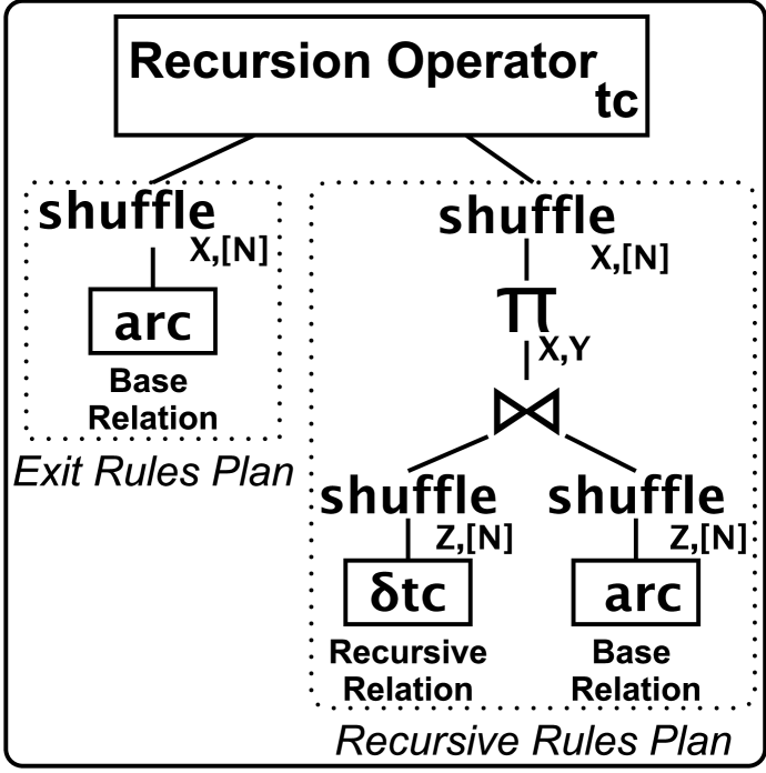
(a) and TC

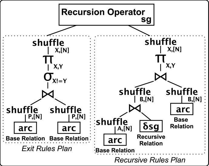
(b) and SG

Figure 2: PSN with SetRDD Physical Plans.

Partitioning.

An earlier research on Datalog showed that a good partitioning strategy (i.e., finding the arguments on which to partition) for a recursive predicate was important for an efficient parallel evaluation [Cohen and Wolfson (1989), Ganguly et al. (1990), Ganguly et al. (1992), Wolfson and Ozeri (1990)]. Since transferring data (i.e., communication) has a high cost in a cluster, we seek a partitioning strategy that limits shuffling. The default partitioning strategy employed by and BigDatalog​​-​​Spark is to partition the recursive predicate on the first argument. Figure 2(2(a)) is the plan for Program 10 for PSN with SetRDD. With the recursive predicate ($\mathtt{t}c$) partitioned on the first argument both the exit rule and recursive rule plans terminate with a shuffle operator.

In the plan in Figure 2(2(a)) $\mathtt{\delta}tc$ requires shuffling prior to the join since it is not partitioned on the join key ($\mathtt{Z}$) because the default partitioning is the first argument ($\mathtt{X}$). However, if the default partitioning strategy was to use instead the second argument, the inefficiency with Figure 2(2(a)) would be resolved but then other programs such as and SG (plan shown in Figure 2(2(b))) would suffer ($\mathtt{\delta}sg$ would require a shuffle prior to the join). Therefore, and BigDatalog​​-​​Spark allows the user to define a recursive predicate’s partitioning via configuration.

Join Optimizations for Linear Recursion.

By keeping the number of partitions static, a shuffle join implementing a linear recursion can have the non-recursive join input cached because the non-recursive inputs will not change during evaluation. This can lead to significant performance improvement since input partitions no longer have to be shuffled and loaded into lookup tables prior to the join in each iteration.

Instead of shuffle joins, each partition of a recursive relation can be joined with an entire relation (e.g., broadcast join). For either type of join, the non-recursive input is loaded into a lookup table. For a broadcast join, the cost of loading the entire relation into a lookup table is amortized over the recursion because the lookup table is cached and then reused in every iteration. Figure 6.3 shows a recursive rules plan for Example 11 ( and SG) with two levels of broadcast joins. In the event that a broadcast relation is used multiple times in a plan, as in Figure 6.3, and BigDatalog​​-​​Spark will broadcast it once and share it among all broadcast join operators joining the relation.

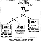
Figure 3: and SG with Broadcast Joins.

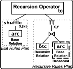
Figure 4: Decomposable and TC Plan.

Decomposable Programs.

Previous research on parallel evaluation of Datalog programs determined that some programs are decomposable and thus evaluable in parallel without redundancy (a fact is only produced once) and without processor communication or synchronization [Wolfson and Silberschatz (1988)]. Since mitigating the cost of synchronization and shuffling can lead to significant execution time speedup, enabling and BigDatalog​​-​​Spark to support techniques for identifying and evaluating decomposable programs is desirable.

We consider a and BigDatalog​​-​​Spark physical plan decomposable if the recursive rules plan has no shuffle operators. Example 10 (linear and TC) is a decomposable program [Wolfson and Silberschatz (1988)] however, its physical plan shown in Figure 2(2(a)) has shuffle operators in the recursive rules plan. Instead, and BigDatalog​​-​​Spark can produce a decomposable physical plan for Example 10. First, $\mathtt{t}c$ will be partitioned by its first argument which divides the recursive relation so that each partition can be evaluated independently and without shuffling. Secondly, a broadcast join will be used which allows each partition of the recursive relation to join with the entire $\mathtt{a}rc$ base relation. Figure 4 is the decomposable physical plan for Example 10. Base relations are not pre-partitioned, therefore the exit rules plan has a shuffle operator to repartition the ${\mathtt{a}rc}$ base relation by ${\mathtt{a}rc}$’s first argument $\mathtt{X}$ into $\mathtt{N}$ partitions.

and BigDatalog​​-​​Spark identifies decomposable programs via syntactic analysis of program rules using techniques presented in the generalized pivoting work [Seib and Lausen (1991)]. The authors of [Seib and Lausen (1991)] show that the existence of a generalized pivot set (GPS) for a program is a sufficient condition for decomposability and present techniques to identify GPS in arbitrary Datalog programs. When a and BigDatalog​​-​​Spark program is submitted to the compiler, the compiler will apply the generalized pivoting solver to determine if the program’s recursive predicates have GPS. If they indeed have, we now have a partitioning strategy and in conjunction with broadcast joins we can efficiently evaluate the program with these settings. For example, Example 10 has a GPS which says to partition the $\mathtt{t}c$ predicate on its first argument. Note that this technique is enabled by using Datalog and it allows and BigDatalog​​-​​Spark to analyze the program at the logical level. The Spark API alone is unable to provide this support since programs are written in terms of physical operations.

6.4 Experiments

In [Shkapsky et al. (2016)] we have tested and BigDatalog​​-​​Sparkover both synthetic and real-world datasets, and compared against other distributed Datalog implementations (e.g., Myria [Halperin et al. (2014)] and SocialLite [Seo et al. (2013)]), as well as hand-coded versions of programs implemented in Spark. The tests were executed using the and TC, and SG, and CC, and PYMK, and and MLMprograms presented in Section 3 plus some additional ones. Here showcase a systems comparison using and TCand and SG(Figure 5) and discuss results of scale-out and scale-up experiments (respectively in Figure 6 and Figure 7). Each execution time reported in the figures is calculated by performing the same experiment five times, discarding the highest and lowest values, and taking the average of the remaining three values. The unit of time measurement is seconds.

Configuration. Our experiments were run on a 16 node cluster. Each node ran Ubuntu 14.04 LTS and had an Intel i7-4770 CPU (3.40GHz, 4 core/8 thread), 32GB memory and a 1 TB 7200 RPM hard drive. Nodes were connected with 1Gbit network. The and BigDatalog​​-​​Sparkimplementation ran on Spark 1.4.0 and the file system is Hadoop 1.0.4.

Datasets. Table 6 shows the synthetic graphs used for the experiments of this section and of Section 7. Tree11 and Tree17 are trees of height 11 and 17 respectively, and the degree of a non-leaf vertex is a random number between 2 and 6. Grid150 is a 151 by 151 grid while Grid250 is a 251 by 251 grid. The Gn-p graphs are n-vertex random graphs (Erdős-Rényi model) generated by randomly connecting vertices so that each pair is connected with probability p. Gn-p graph names omitting p use default probability 0.001. Note that for these graphs and TC and and SG are capable of producing result sets many orders of magnitude larger than the input dataset, as shown by the last two columns in Table 6.

Table 6: Parameters of Synthetic Graphs

Name	Vertices	Edges	and TC	and SG
Tree11	71,391	71,390	805,001	2,086,271,974
Tree17	13,766,856	13,766,855	237,977,708
Grid150	22,801	45,300	131,675,775	2,295,050
Grid250	63,001	125,500	1,000,140,875	10,541,750
G5K	5,000	24,973	24,606,562	24,611,547
G10K	10,000	100,185	100,000,000	100,000,000
G10K-0.01	10,000	999,720	100,000,000	100,000,000
G10K-0.1	10,000	9,999,550	100,000,000	100,000,000
G20K	20,000	399,810	400,000,000	400,000,000
G40K	40,000	1,598,714	1,600,000,000	1,600,000,000
G80K	80,000	6,399,376	6,400,000,000	6,400,000,000

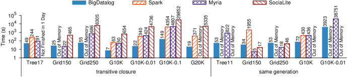
Figure 5: System Comparison using and TCand and SG.

Systems Comparison. For and TC, and BigDatalog​​-​​Spark uses Program 10 with the decomposed plan from Figure 4. For and SG, and BigDataloguses Program 11 with broadcast joins (Figure 6.3). We use equivalent programs in Myria and Socialite, and hand-optimized semi-naïve programs written in the Spark API which are implemented to minimize shuffling. Figure 5 shows the evaluation time for all four systems.

and BigDatalog​​-​​Spark is the only system that finishes the evaluation for and TC and and SG on all graphs except and SG on Tree17 since the size of the result is larger than the total disk space of the cluster. and BigDatalog​​-​​Spark has the fastest execution time on six of the seven graphs for and TC; on four of the graphs it outperforms the other systems by an order of magnitude. The and BigDatalog​​-​​Spark plan only performs an initial shuffle of the dataset, and then evaluates the recursion without shuffling, and proves very efficient. In the case of Grid150, which is the smallest graphs used in this experiment in terms of both edges and queries output sizes, Myria outperforms and BigDatalog​​-​​Sparkboth in and TCand and SG. This is explained as the evaluation requires many iterations, where each iteration performs very little work, and therefore the overhead of scheduling in and BigDatalog​​-​​Spark takes a significant portion of execution time. However, as the data set becomes larger the superior scalability of and BigDatalog​​-​​Sparkcomes into play enabling it to outperform all other systems on Grid250. In fact, Figure 5 shows that the execution time of and BigDatalog​​-​​Sparkon and TConly grows to 2.2 times those of Grid150, whereas those of Myria and Socialite grow by more than one order of magnitude; from Grid150 to Grid250, and BigDatalog​​-​​Sparkalso scales better on and SGcompared to the other systems. The Spark programs are not only affected by the overhead of scheduling and shuffling, but also suffer memory utilization issues related to dataset caching, and therefore ran out of memory for several datasets both in and TCand and SG.

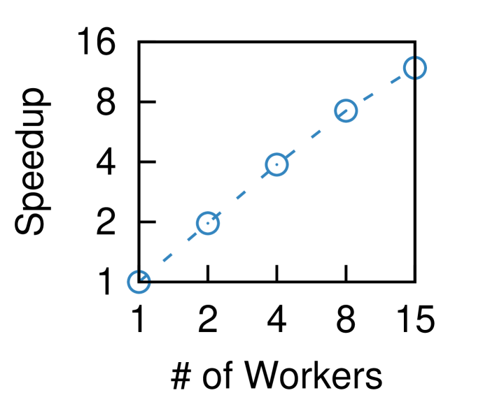
(a) and TCon G20K

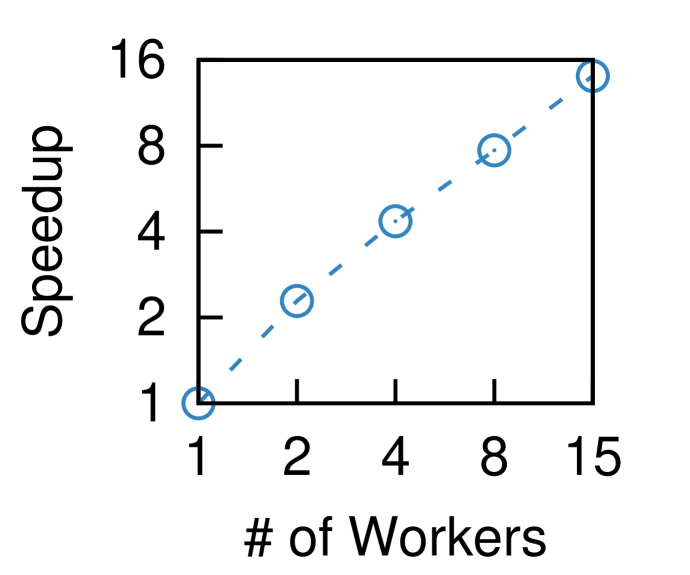
(b) and SGon G10K

Figure 6: Scaling-out Cluster Size.

Scalability. In this set of experiments we use the Gn-p graphs. Figure 6(6(a)) shows the speedup for and TC on G20K as the number of workers increases from one to 15 (all with one master) w.r.t. using only one worker, and Figure 6(6(b)) shows the same experiment run for and SG with G10K. Both figures show a linear speedup, with the speedup of using 15 workers as 12X and 14X for and TC and and SG, respectively.

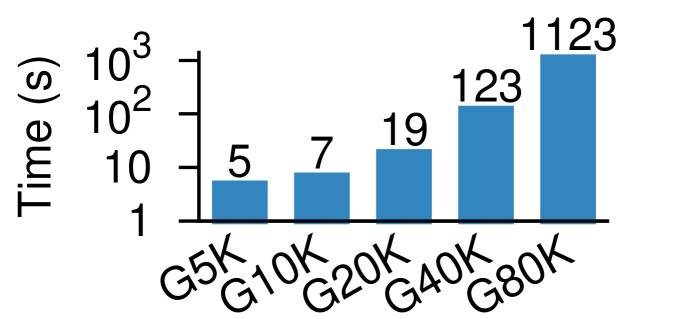
(a) and TC

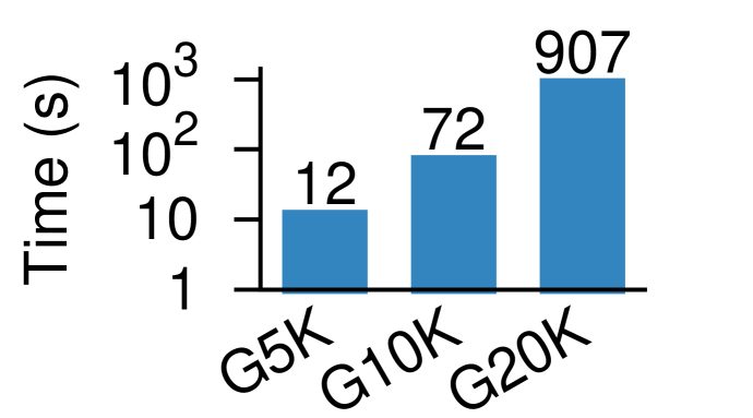
(b) and SG

Figure 7: Scaling-up on Random Graphs.

The scaling-up results shown in Figure 7 were ran with the full cluster, i.e., one master and 15 workers. With each successively larger graph size, i.e., from G5K to G10K, the size of the transitive closure quadruples, but we do not observe a quadrupling of the evaluation time. Instead, evaluation time increases first less than 1.5X (G5K to G10K), then 3X (G10K to G20K), 6X (G20K to G40K), and 9X (G40K to G80K). Rather than focusing on the size of the and TC w.r.t. execution time, the reason for the increase in execution time is explained by examining the results in Table 7.

Table 7:   and TC Scaling-up Experiments Result Details

(Execution time not including the time to broadcast $\mathtt{a}rc$)  Graph Time - and TC Generated Facts Generated Generated broadcast(s) Facts / and TC Facts / Sec. G5K 4 24,606,562 122,849,424 4.99 30,712,356 G10K 6 100,000,000 1,001,943,756 10.02 166,990,626 G20K 17 400,000,000 7,976,284,603 19.94 469,193,212 G40K 119 1,600,000,000 50,681,485,537 31.68 425,894,836 G80K 1112 6,400,000,000 510,697,190,536 79.80 459,673,439  

Broadcasting the $\mathtt{a}rc$ relation requires between one second for G5K to twelve seconds for G80K. Table 7 shows the execution time minus the time to broadcast $\mathtt{a}rc$, which is the total time the program required to actually evaluate and TC. Table 7 also shows the number of generated facts, which is the number of total facts produced prior to de-duplication and is representative of the actual work the system must perform to produce the and TC(i.e., HashSet lookups), the ratio between and TC size and generated facts, and the number of generated facts per second (time - broadcast time), which should be viewed as the evaluation throughput. These details help to explain why the execution times increase at a rate greater than the increase in and TC size – the number of generated facts is increasing at a rate much greater than the increase in and TC size. The last column shows that even with the increase in number of generated facts, and BigDatalog​​-​​Spark still maintains good throughput throughout. Continuing, the first two graphs are too small to stress the system, but once the graph is large enough (e.g., G20K) the system exhibits a much greater throughput, which is stable across the larger graphs.

Table 8: and SGScaling-up Experiments Result Details

(Execution time not including the time to broadcast $\mathtt{a}rc$)  Graph Time - and SG Generated Facts Generated Generated broadcast(s) Facts / and SG Facts / Sec. G5K 11 24,611,547 612,891,161 24.90 55,717,378 G10K 71 100,000,000 10,037,915,957 100.38 141,379,098 G20K 905 400,000,000 159,342,570,063 398.36 176,069,138  

Table 8 displays the same details as Table 7 but for and SG. Table 8 displays the execution time-minus the broadcast time of $\mathtt{a}rc$, the result set size, the number of generated facts as well as statistics for the ratio of generated facts for each and SG fact and generated fact per second of evaluation (throughput). With and SG, the number of generated facts is much higher than we observe with and TC, reflecting the greater amount of work and SG requires. For example, on G10K and G20K  and SG produces 10X and 20X the number of generated facts, respectively, than and TC produces. We also observe a much greater rate of increase in generated facts between graph sizes for and SG compared to and TC. For example, from G10K to G20K we see a 16X increase in generated facts for and SG versus only an 8X increase for and TC. For and SG, we do not achieve as high a throughput as with and TC, which is explained in part by the fact that and SG requires shuffling, whereas our and TC program evaluates purely in main memory after an initial shuffle.

7 Datalog on Multicore Systems: and BigDatalog​​-​​MC

Multicore machines are composed by one or more processors, where each of them contains several cores on a chip [Venu (2011)]. Each core is composed of computation units and caches, while the main memory is commonly shared. While the individual cores do not necessarily run as fast as the highest performing single-core processors, they are able to obtain high performance by handling more tasks in parallel. In this paper we will consider multicore processors implemented as a group of homogeneous cores, where the same computation logic is applied in a divide-and-conquer way over a partition of the input dataset.

Unfortunately, single-core applications do not get faster automatically on a multicore architecture with the increase of cores. For this reason, programmers are forced to write specific parallel logic to exploit the performance of multicore architectures. Next we present the techniques used by and BigDatalog​​-​​MCto enable the efficient parallel evaluation of Datalog programs over a shared-memory multicore machine with $n$ processors.

7.1 Parallel Bottom-Up Evaluation

We start with how and BigDatalog​​-​​MCperforms the parallel bottom-up evaluation of the transitive closure program and TCin Example 10. We divide each relation into $n$ partitions and we use the relation name with a superscript $i$ to denote the $i$-th partition of the relation. Each partition has its own storage for tuples, unique index, and secondary indexes. Assuming that there are $n$ workers that perform the actual query evaluation, and one coordinator that manages the coordination between the workers. Example 12 below shows a parallel evaluation plan for and TC.

Example 12 (Parallel bottom-up evaluation of and TC)

Let $h$ be a hash function that maps a vertex to an integer between 1 to $n$. Both ${\mathtt{a}rc}$ and ${\mathtt{t}c}$ are partitioned by the first column, i.e., $h({\mathtt{X}})=i$ for each ${\mathtt{(}X,Y)}$ in ${\mathtt{a}rc}^{i}$ and $h({\mathtt{X}})=i$ for each ${\mathtt{(}X,Y)}$ in ${\mathtt{t}c}^{i}$. The parallel evaluation proceeds as follows.

1. The $i$-th worker evaluates the exit rule by adding a tuple ${\mathtt{(}X,Y)}$ to ${\mathtt{t}c}$ for each tuple ${\mathtt{(}X,Y)}$ in ${\mathtt{a}rc}^{i}$.

2. Once all workers finish Step (1), the coordinator notifies each worker to start Step (3).

3. For each new tuple ${\mathtt{(}X,Z)}$ in ${\mathtt{t}c}^{i}$ derived in the previous iteration, the $i$-th worker looks for tuples of the form ${\mathtt{(}Z,Y)}$ in ${\mathtt{a}rc}$ and adds a tuple ${\mathtt{(}X,Y)}$ to ${\mathtt{t}c}$.

4. Once all workers finish Step (3), the coordinator checks if the evaluation for ${\mathtt{t}c}$ is completed. If so, the evaluation terminates; otherwise, the evaluation starts from Step (3).

In Step (1) and Step (3), each worker performs its task on one processor while the coordinator waits. Step (2) and Step (4) serve as synchronization barriers.

In the above example, the $i$-th worker only writes to ${\mathtt{t}c}^{i}$ in Step (1), and it only reads from and writes to ${\mathtt{t}c}^{i}$ in Step (3). Thus, ${\mathtt{t}c}^{i}$ is only accessed by the $i$-th worker. This property does not always hold in every evaluation plan of ${\mathtt{t}c}$. For example, if we keep the current partitioning for ${\mathtt{a}rc}$ but instead partition ${\mathtt{t}c}$ by its second column, then every worker could write to ${\mathtt{t}c}^{i}$ in Step (3), and multiple write operations to ${\mathtt{t}c}^{i}$ can occur concurrently; in this plan, we use a lock to ensure only one write operation to ${\mathtt{t}c}^{i}$ is allowed at a time—a worker needs to acquire the lock before it writes to ${\mathtt{t}c}^{i}$, and it releases the lock once the write operation completes.

In general, we use a lock to control the access to a partition if multiple read/write operations can occur concurrently. There are two types of locks: (i) an exclusive lock (x-lock) that allows only one operation at a time; and (ii) a readers–writer lock (rw-lock) that a) allows only one write operation at a time, b) allows concurrent read operations when no write operation is being performed, and c) disallows any read operation when a write operation is being performed. We use (i) an x-lock if there is no read operation and only multiple write operations can occur concurrently; (ii) an rw-lock if multiple read and write operations can occur concurrently since it allows for more parallelism than an x-lock.

We assume that every relation is partitioned using the same hash function $h$ defined as

$$h(x_{1},\ldots,x_{t})=\sum_{i=1}^{t}g(x_{i})\bmod n,$$

where the input to $h$ is a tuple of any arity $t$ and $g$ is a hash function with a range no less than $n$. Then the key factor that determines whether locks are required during the evaluation is how each relation is partitioned, which is specified using discriminating sets. A discriminating set of a (non-nullary) relation $R$ is a non-empty subset of columns in $R$. Given a discriminating set of a relation, we divide the relation into $n$ partitions by the hash value of the columns that belong to the discriminating set. For each predicate $p$ that corresponds to a base relation or a derived relation, let $R$ be the relation that stores all tuples corresponding to facts about $p$ in memory; we select a discriminating set of $R$ that specifies the partitioning of $R$ used in the evaluation of $p$. The collection of all the selected discriminating sets uniquely determines how each relation is partitioned. These discriminating sets can be arbitrarily selected as long as there is a unique discriminating set for each derived relation.

Example 13 (Discriminating sets for the plan in Example 12)

The discriminating sets for the two occurrences of ${\mathtt{a}rc}$ are both $\{1\}$. Moreover, ${\mathtt{t}c}$ is a derived relation, and its discriminating set is $\{1\}$.

7.2 Parallel Evaluation of AND/OR Trees

The internal representation used by and BigDatalog​​-​​MCto represent a Datalog program is an AND/OR tree [Arni et al. (2003)]. An OR node represents a predicate and an AND node represents the head of a rule. The root is an OR node. The children of an OR node (resp., AND node) are AND nodes (resp., OR nodes). Each node has a ${\mathtt{g}etTuple}$ method that calls the ${\mathtt{g}etTuple}$ methods of its children. Each successful invocation to the method instantiates the variables of one child (resp., all the children) and the parent itself for an OR node (resp., AND node). The program is evaluated by repeatedly applying the ${\mathtt{g}etTuple}$ method upon its root until it fails. Thus, for an OR node, the execution (i) exhausts the tuples from the first child; (ii) continues to the next child; and (iii) fails when the last child fails. An OR node is an R-node if it reads from a base or derived relation with its ${\mathtt{g}etTuple}$ method, while it is a W-node if it writes to a derived relation with its ${\mathtt{g}etTuple}$ method. Finally, an OR node is an entry node if (i) it is a leaf, and (ii) it is the first R-node among its siblings, and (iii) none of its ancestor OR nodes has a left sibling (i.e., a sibling that appears before the current node) that has an R-node descendant or a W-node descendant.

Example 14 (AND/OR tree of and SG)

Figure 8 shows the adorned AND/OR tree of the same generation program and SGin Example 11, where (i) the text inside a node indicates its type and ID, e.g., “Or-1” indicates that the root is an OR node with ID 1, and (ii) the text adjacent to a node shows the corresponding predicate with its adornment (${\mathtt{b}}$ or ${\mathtt{f}}$ in the $i$-th position means the $i$-th argument in a predicate $p$ is bound or free when $p$ is evaluated). Thus, Or-4, Or-5, Or-7, Or-8, and Or-9 are R-nodes, and Or-1 is a W-node. Or-4 and Or-7 are entry nodes in this program. Although Or-5 is an R-node, it is not an entry node since it is not the first R-node among its siblings. Similarly for Or-8 and Or-9.

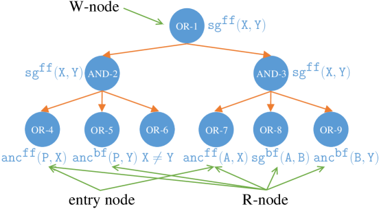
Figure 8: AND/OR tree of and SGprogram in Example 11.

In the parallel evaluation of an AND/OR tree with one coordinator and $n$ workers, we create $n$ copies of the same AND/OR tree, and assign the $i$-th copy to the $i$-th worker. The evaluation is divided into $n$ disjoint parts, where the $i$-th worker evaluates an entry node by instantiating variables with constants from the $i$-th partition of the corresponding relation, while it has full access to all partitions of the corresponding relations for the remaining R-nodes. The parallel evaluation ensures the same workflow as the sequential pipelined evaluation by adding synchronization barriers in the nodes that represent recursion. For example, we create a synchronization barrier $B$, and add it to Or-1 of Figure 8 for every copy of the AND/OR tree. Now, the evaluation works as follows.

1. Each worker evaluates the exit rule by calling And-2.getTuple until it fails. A worker waits at $B$ after it finishes.

2. Once all $n$ workers wait at $B$, the coordinator notifies each worker to start Step (3).

3. Each worker evaluates the recursive rule by calling And-3.getTuple until it fails. A worker waits at $B$ after it finishes.

4. Once all $n$ workers wait at $B$, the coordinator checks if there are new tuples derived in ${\mathtt{s}g}$. If so, the evaluation continues from Step (3); otherwise, the evaluation terminates.

7.3 Selecting a Parallel Plan

and BigDatalog​​-​​MCuses a technique called Read/Write Analysis (RWA) [Yang et al. (2017)] to help find the best discriminating sets to evaluate a program. For a given set of discriminating sets, the RWA on an adorned AND/OR tree determines the actual program evaluation plan, including the type of lock needed for each derived relation, whether an OR node needs to acquire a lock before accessing the corresponding relation, and which partition of the relation an OR node needs to access when it accesses the relation through index lookups. The analysis performs a depth-first traversal on the AND/OR tree that simulates the actual evaluation to check each read or write operation performed by the $i$-th worker. For each node $N$ encountered during the traversal, the following three cases are possible:

1. $N$ is an entry node. In this case, set it as the current entry node; then, for each W-node that is an ancestor of $N$ and is in the same stratum as $N$, determine whether the $i$-th worker only writes to the $i$-th partition of $R(p_{w})$. This is done by checking if $p_{e}[\overline{X_{j}}]=p_{w}[\overline{X_{k}}]$, where $p_{e}$ and $p_{w}$ are the predicates associated with $N$ and the W-node, respectively, and $\overline{X_{j}}$ and ${\overline{X_{k}}}$ are the corresponding discriminating sets.

2. $N$ is an R-node that reads from a derived relation. In this case, determine whether the $i$-th worker only reads from the $i$-th partition of $R(p_{r})$ by checking if $\overline{X_{k}}\subseteq\overline{B}$ and $p_{e}[\overline{X_{j}}]=p_{r}[\overline{X_{k}}]$, where $p_{e}$ and $p_{r}$ are the predicates associated with the current entry node and $N$, respectively, $\overline{X_{j}}$ and ${\overline{X_{k}}}$ are the corresponding discriminating sets, and $\overline{B}$ is the set of positions for bound arguments in $N$.

3. $N$ is an R-node that reads from a base relation through a secondary index. In this case, determine whether the $i$-th worker only needs to read from one partition of $R(p_{r})$ instead of all the partitions by checking if $\overline{X_{k}}\subseteq\overline{B}$, where $p_{r}$ is the predicate associated with $N$, ${\overline{X_{k}}}$ is the corresponding discriminating set, and $\overline{B}$ is the set of positions for bound arguments in $N$.

We can formulate the problem of determining the best discriminating sets for a given program as an optimization problem that minimizes the cost of program evaluation. This is equivalent to minimizing the overhead of program evaluation over the “ideal” plan in which all the constraints are satisfied. Now, for each OR node $N$ in the AND/OR tree, its contribution to the overhead of program evaluation is denoted by $c(N)$, and its value is heuristically set as follows:

$$c(N)=\left\{\begin{array}[]{ll}3,&\mbox{if}~{}N~{}\mbox{needs to acquire an r-lock (read lock) before performing an}\\ &\mbox{index lookup and condition}~{}\overline{X_{k}}\subseteq\overline{B}~{}\mbox{is violated};\\ 1,&\mbox{if}~{}N~{}\mbox{needs to acquire a write lock before accessing the relation};\\ 0,&\mbox{otherwise}.\end{array}\right.$$

Thus, the optimization problem reduces to finding an assignment that minimizes $\sum_{N}c(N)$, where $N$ iterates over the set of OR nodes in the AND/OR tree. In and BigDatalog​​-​​MC, this is achieved by enumerating all possible assignments using brute force, since the number of such valid assignments is totally tractable for most recursive queries of our interest. It is also important to take a closer look at the case where $c(N)$ equals three. There are two parts in the corresponding condition: first, $N$ needs to acquire a read lock before performing an index lookup, and second, condition $\overline{X_{k}}\subseteq\overline{B}$ is violated. When $\overline{X_{k}}\subseteq\overline{B}$ is not true, this means we need to perform a lookup for each partition. This cost should be at least two, as there should be more than one partition during the parallel evaluation (otherwise, there is no need for parallelizing as there is only one partition and one processor). We also need to acquire a read lock for each lookup. However, we do not want to penalize this as much as acquiring a write lock, as acquiring a read lock is relatively less expensive. So the contribution from the read lock is counted as one, and the overall cost is summed as three.

7.4 Experiments

Now we introduce a set of experiments showcasing the performance of and BigDatalog​​-​​MCcompared to other (single and multicore) Datalog implementations, namely LogicBlox [Aref et al. (2015)], DLV [Leone et al. (2006)], clingo [Gebser et al. (2014)], and SociaLite [Seo et al. (2013)]. Additional experiments and details can be found in [Yang et al. (2017)].

Configuration. We tested the performance of the above systems on a machine with four AMD Opteron 6376 CPUs (16 cores per CPU) and 256GB memory (configured into eight NUMA regions). The operating system was Ubuntu Linux 12.04 LTS. We used LogicBlox 4.1.9 and clingo version 4.5.0. The version of DLV we used is a single-processor version , while for SociaLite we used the parallel version that was downloaded from https://github.com/socialite-lang/socialite.

System Comparison. Figure 9 compares the evaluation time of the five systems on and TC, and SG, and and ATTENDquery. Bars for DLV and BDLog-1 show the evaluation time of DLV and and BigDatalog​​-​​MCusing one processor, while bars for LogicBlox, Clingo, SociaLite, and BDLog-64 show the evaluation time of those systems over 64 processors. In our experiments, we observed both SociaLite and and BigDatalog​​-​​MChad higher CPU utilization most of the time, as compared to LogicBlox and clingo, with the latter utilizing only one processor most of the time.

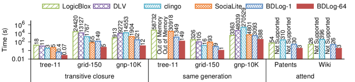
Figure 9: Query evaluation time of recursive queries.

When and BigDatalog​​-​​MCis allowed to use only one processor, it always outperforms DLV and clingo. This comparison suggests that and BigDatalog​​-​​MCprovides a tighter implementation compared with the other two systems; specifically, we found that clingo, although a multicore Datalog implementation, spends most of the time on the grounder that utilizes only one processor.

Moreover, with only one processor, and BigDatalog​​-​​MCoutperforms or is on par with LogicBlox and SociaLite, while LogicBlox and SociaLite are allowed to use all 64 processors. Naturally, and BigDatalog​​-​​MCalways significantly outperforms LogicBlox and SociaLite when it uses all 64 processors. The performance gap between LogicBlox and and BigDatalog​​-​​MCis largely due to the staged evaluation used by LogicBlox, which stores all the derived tuples in an intermediate relation, and performs deduplication or aggregation on the intermediate relation. For the evaluation that produces large amount duplicate tuples, such as ${\mathtt{T}C}$ on Grid150 and ${\mathtt{S}G}$ on Tree11, this strategy incurs a high space overhead, and the time spent on the deduplication, which uses only one processor, dominates the evaluation time. SociaLite instead uses an array of hash tables with an initial capacity of around 1,000 entries for a derived relation, whereas and BigDatalog​​-​​MCuses an append-only structure to store the tuples and a B+ tree to index the tuples. Although the cost of accessing a hash table is lower than that of a B+ tree, the design adopted by and BigDatalog​​-​​MCallows a better memory allocation pattern as the relation grows. Such overhead is amplified when (i) multiple processors try to allocate memory at the same time, or (ii) the system has a high memory footprint.

Lastly, note that and BigDatalog​​-​​MCachieves a greater speedup (the speedup of BDLog-64 over BDLog-1) for ${\mathtt{T}C}$ than ${\mathtt{S}G}$ and ${\mathtt{A}TTEND}$ since no lock is used in ${\mathtt{T}C}$, while ${\mathtt{S}G}$ and ${\mathtt{A}TTEND}$ suffer from lock contention.

8 Related Work

Datalog Semantics. Supporting aggregates in recursion is an old and difficult problem which has been the topic of much previous research work. Remarkably, previous approaches had primarily focused on providing a formal semantics that could accommodate the non-monotonic nature of the aggregates. In particular [Mumick et al. (1990)] discussed programs that are stratified w.r.t. aggregates operators and proved that a perfect model exists for these programs. Then, [Kemp and Stuckey (1991)] defined extensions of the well-founded semantics to programs with aggregation, and later showed that programs with aggregates might have multiple and counter-intuitive stable models. The notion of cost-monotonic extrema aggregates was introduced by [Ganguly et al. (1995)], using perfect models and well-founded semantics, whereas  [Greco et al. (1992)] showed that their use to express greedy algorithms requires the don’t-care non-determinism of the stable-model semantics provided by the choice construct. An approach to optimize programs with extrema was proposed by [Ganguly et al. (1991)], and a general optimization technique based on an early pruning of non-relevant facts was proposed by Sudarshan et al. [Sudarshan and Ramakrishnan (1991)].

A general approach to deal with the four aggregates, min, max, count and sum, in a unified framework was proposed by [Ross and Sagiv (1992)] who advocated the use of semantics based on specialized lattices, different from set-containment, whereby each aggregate will then define a monotonic mapping in its specialized lattice. However several limitations of this proposal were pointed out by Van Gelder [Van Gelder (1993)], including the assumption that cost arguments of atoms are functionally dependent from the other arguments. This is a property that does not hold in many applications and it also difficult to determine, since determining if a derived predicate satisfies a functional dependency is undecidable in general [Abiteboul and Hull (1988)]. In the following years, interest in aggregates for logic-based systems focused on their use in the framework of Answer-Sets [Erdem et al. (2016)] which is less conducive to Big Data applications.

A renewed interest in Big Data analytics brought a revival of Datalog for expressing more powerful data-intensive algorithms—including many that require aggregates in recursion. At UCLA, researchers first introduced the notion of monotonic sum and count [Mazuran et al. (2013b), Mazuran et al. (2013a)] and then proposed the comprehensive solution that is described in this paper and covers all four basic aggregates along with efficient techniques for their efficient and scalable implementation.

Datalog Implementations. The Myria [Wang et al. (2015)] runtime supports Datalog evaluation using a pipelined, parallel, distributed execution engine that evaluates graph of operators. Datasets are sharded and stored in PostgreSQL instances at worker nodes. SociaLite [Seo et al. (2013)] is a Datalog language implementation for social network analysis. SociaLite programs are evaluated by parallel workers that use message passing to communicate. Both SociaLite and Myria support aggregation inside recursion focusing on their operational semantics. The lattice-based approach of Ross and Sagiv [Ross and Sagiv (1992)] is proposed as the possible basis for a declarative semantics, but no approach on how to overcome its limitations is discussed. Furthermore, the advent of graphics processing units (GPUs) has recently led to Datalog implementations on GPUs for relational learning algorithms [Martínez-Angeles et al. (2016)]. Since the transfer of data between host and GPU memory incurs in significant cost, Datalog implementations on GPUs [(47)] optimize this cost through efficient memory management schemes.

Parallel Datalog Evaluation and Languages. Previous research on parallel evaluation of Datalog programs determined that some programs are evaluable in parallel without redundancy and without processor communication or synchronization [Wolfson and Silberschatz (1988)]. Such programs are called decomposable. Our parallel implementations identify decomposable programs via syntactic analysis of program rules using the generalized pivoting method [Seib and Lausen (1991)]. Others have also explored the idea of applying extensions of simple 0-1 laws on Datalog programs to derive at a parallelization plan that maximizes the expected performance [Lifschitz and Vianu (1998)].

Many works produced over twenty years ago focused on parallelization of bottom-up evaluation of Datalog programs [Zhang et al. (1995)], however they were largely of a theoretical nature. For instance [Van Gelder (1993)] proposed a message passing framework for parallel evaluation of logic programs. Techniques to partition program evaluation efficiently among processors [Wolfson and Ozeri (1990)], the trade-off between redundant evaluation and communication [Ganguly et al. (1990), Ganguly et al. (1992)], and classifying how certain types of Datalog programs can be evaluated [Cohen and Wolfson (1989)] were also studied. A parallel semi-naïve fixpoint has been proposed for message passing [Wolfson and Ozeri (1990)] that includes a step for sending and receiving tuples from other processors during computation. The PSN used in this work applies the same program over different partitions and shuffle operators in place of processor communication. Parallel processing of recursive queries in particular is also a well-studied problem. One such example is [Bell et al. (1991)], where the recursive query is first transformed into a canonical form and then evaluated in a pipelined fashion.

Recently, Semantic Web reasoning systems dealing with RDF data has utilized this early research in parallel implementations of semi-naïve evaluation [Abiteboul et al. (1995)] to handle recursive Datalog rules much like commercial systems as LogicBlox. One such system is RDFox [Motik et al. (2014)] which is a main-memory, multi-core RDF system that uses a specialized RDF indexing data structure to ensure largely lock-free concurrent updates. It is also important to mention in this regard that, with the emergence of large Knowledge Graphs [Urbani et al. (2016)], the Semantic Web community has significantly contributed to the ongoing research in Datalog reasoning. In fact, many reasoning systems encode RDF data, as represented in Knowledge Graphs, into ternary database predicates for writing elegant Datalog rules, which in turn, have to be efficiently evaluated. One such recent system is Vlog [Urbani et al. (2016)] which exploits column-based memory layout along with selective caching of certain subquery results. However, Vlog is intrinsically sequential in nature and does not have a parallel or distributed implementation.

Among the distributed Datalog languages, it is noteworthy to mention OverLog [Loo et al. (2005), Condie et al. (2008)], used in the P2 system to express overlay networks, and NDlog [Loo et al. (2006)] for declarative networking. The Bloom^L [Conway et al. (2012)] distributed programming language uses various monotonic lattices, also based on the semantics of [Ross and Sagiv (1992)], to identify program elements not requiring coordination. [Bu et al. (2012)] showed how XY-stratified Datalog can support computational models for large-scale machine learning, although no full Datalog language implementation on a large-scale system was provided.

Beyond Datalog: Parallel Execution of Logic Programs. In logic programming, programs are evaluated in a top-down fashion through unification. An extensive body of research was produced on parallel logic programming, dating back to 1981 [Gupta et al. (2001), de Kergommeaux and Codognet (1994)]). Two major approaches exists for parallelizing logic programs: the implicit approach assumes that the framework is able to parallelize the given input program automatically without any programmer intervention. Conversely, in the explicit case specific constructs are introduced into the source language to guide the parallel evaluation. The approach used in our and BigDatalogsystems is implicit parallelism where any input Datalog program is automatically parallelized by the runtime.

In implicit parallel logic programming, three main forms of parallelism exists: (i) And-Parallelism whereby multiple literals are evaluated concurrently; (2) Or-Parallelism where instead clauses are evaluated in parallel; and (3) Unification Parallelism in which the unification process is parallelized. Our parallel evaluation of Datalog programs is a form of Or-Parallelism where data is partitioned such that different rule instantiations are evaluated concurrently.

It is also important to note that the growth of Semantic Web data also propelled considerable research on large-scale reasoning on distributed frameworks like MapReduce [Dean and Ghemawat (2004)]. One such example is the WebPIE system [Urbani et al. (2012)] that implements forward reasoning for RDFS over MapReduce framework. The key ideas originating from distributed MapReduce frameworks used for Semantic Web reasoning were also applied for description logic $\mathcal{EL}^{+}$ [Mutharaju et al. (2010)] for $\mathcal{EL}^{+}$ ontology classifications. In this era of big data, the Semantic Web community also led considerable research efforts towards large-scale non-monotonic reasoning of RDF data. One such paper is [Tachmazidis et al. (2012)] which proposed a MapReduce based parallel framework for defeasible logic and predicates of any arity in presence of noisy data. In the same vein of large scale non-monotonic reasoning, the authors of [Tachmazidis et al. (2014)] proposed a similar data parallel MapReduce framework for well-founded semantics computation through efficient implementations of joins and anti-joins.

9 Conclusion

By embracing the Horn-clause logic of Prolog but not its operational constructs such as the cut, Datalog researchers, 30 years ago, embarked in a significant expedition toward declarative languages in which logic alone rather than Logic+Control [Kowalski (1979)] can be used to specify algorithms. Significant progress toward this ambitious goal was made in the 90s with techniques such as semi-naïve fixpoint and magic sets that support recursive Datalog programs by bottom-up computation and implementation techniques from relational DB systems. As described in Section 8, however, declarative semantics for algorithms that require aggregates in recursion largely remained an unsolved problem for this first generation of deductive DB systems. Moreover, Datalog scalability via parallelization was only discussed in papers, until recently when the availability of new parallel platforms and an explosion of interest in BigData renewed interest in Datalog and its parallel implementations on multicore and distributed systems.

In this paper, we have provided an in-depth description of the UCLA’a BigDatalog/DeAL project that is of significance because of its (i) historical continuity with first-generation Datalog systems ($\mathcal{}LDL{++}$ was supported and extended at UCLA for several years [Arni et al. (2003)]), (ii) implementation on multiple platforms, with levels of performance that surpass those of competing Datalog systems, GraphX applications, and even Apache Spark applications written in Scala, and (iii) support for a wide range of declarative algorithms using the rigorous non-monotonic semantics for recursive programs with aggregates introduced in [Zaniolo et al. (2017)].

Furthermore, we believe that the use of aggregates in recursive rules made possible by $\mathcal{}P$$\!reM$ [Zaniolo et al. (2017)] can lead to beneficial extensions in several application areas, e.g., KDD algorithms, and in related logic-based systems, including, e.g., those that use tabled logic programming [Swift and Warren (2012)] and Answer Sets [Erdem et al. (2016)]. Therefore we see many interesting new topics deserving further investigation, suggesting that logic and databases remains a vibrant research area [Zaniolo et al. (2018)] although many years have passed since it was first introduced [Minker et al. (2014)].

References

- Abiteboul and Hull (1988) Abiteboul, S. and Hull, R. 1988. Data functions, datalog and negation (extended abstract). In Proceedings of the 1988 ACM SIGMOD International Conference on Management of Data, Chicago, Illinois, June 1-3, 1988. 143–153.
- Abiteboul et al. (1995) Abiteboul, S., Hull, R., and Vianu, V., Eds. 1995. Foundations of Databases: The Logical Level, 1st ed. Addison-Wesley Longman Publishing Co., Inc., Boston, MA, USA.
- Agrawal et al. (1994) Agrawal, R., Srikant, R., et al. 1994. Fast algorithms for mining association rules. In Proceedings of the 20th International Conference on Very Large Data Bases. Vol. 1215. 487–499.
- Ameloot et al. (2011) Ameloot, T. J., Neven, F., and Van den Bussche, J. 2011. Relational transducers for declarative networking. In PODS. 283–292.
- Aref et al. (2015) Aref, M., ten Cate, B., Green, T. J., Kimelfeld, B., et al. 2015. Design and implementation of the logicblox system. In SIGMOD. ACM, 1371–1382.
- Armbrust et al. (2015) Armbrust, M., Xin, R. S., Lian, C., Huai, Y., Liu, D., Bradley, J. K., Meng, X., Kaftan, T., Franklin, M. J., Ghodsi, A., and Zaharia, M. 2015. Spark SQL: Relational Data Processing in Spark. In SIGMOD. 1383–1394.
- Arni et al. (2003) Arni, F., Ong, K., Tsur, S., Wang, H., and Zaniolo, C. 2003. The deductive database system LDL++. TPLP 3, 1, 61–94.
- Bell et al. (1991) Bell, D. A., Shao, J., and Hull, M. E. C. 1991. A pipelined strategy for processing recursive queries in parallel. Data & Knowledge Engineering 6, 5, 367–391.
- Borkar et al. (2012) Borkar, V. R., Bu, Y., Carey, M. J., Rosen, J., et al. 2012. Declarative systems for large-scale machine learning. IEEE Data Eng. Bull. 35, 2, 24–32.
- Borkar et al. (2011) Borkar, V. R., Carey, M. J., Grover, R., Onose, N., and Vernica, R. 2011. Hyracks: A flexible and extensible foundation for data-intensive computing. In ICDE. 1151–1162.
- Bu et al. (2012) Bu, Y., Borkar, V. R., Carey, M. J., Rosen, J., Polyzotis, N., Condie, T., Weimer, M., and Ramakrishnan, R. 2012. Scaling datalog for machine learning on big data. CoRR abs/1203.0160.
- Cardoso et al. (2009) Cardoso, J. C., Baquero, C., and Almeida, P. S. 2009. Probabilistic estimation of network size and diameter. In Fourth Latin-American Symposium on Dependable Computing (LADC’09). IEEE, 33–40.
- Chimenti et al. (1987) Chimenti, D., O’Hare, A. B., Krishnamurthy, R., Tsur, S., West, C., and Zaniolo, C. 1987. An overview of the LDL system. IEEE Data Eng. Bull. 10, 4, 52–62.
- Cohen and Wolfson (1989) Cohen, S. and Wolfson, O. 1989. Why a single parallelization strategy is not enough in knowledge bases. In PODS. 200–216.
- Condie et al. (2008) Condie, T., Chu, D., Hellerstein, J. M., and Maniatis, P. 2008. Evita raced: metacompilation for declarative networks. PVLDB 1, 1 (Aug.), 1153–1165.
- Conway et al. (2012) Conway, N., Marczak, W. R., Alvaro, P., Hellerstein, J. M., and Maier, D. 2012. Logic and lattices for distributed programming. In ACM Symposium on Cloud Computing, SOCC ’12, San Jose, CA, USA, October 14-17, 2012.
- Das and Zaniolo (2016) Das, A. and Zaniolo, C. 2016. Fast lossless frequent itemset mining in data streams using crucial patterns. In Proceedings of the 2016 SIAM International Conference on Data Mining, Miami, Florida, USA, May 5-7, 2016. 576–584.
- de Kergommeaux and Codognet (1994) de Kergommeaux, J. C. and Codognet, P. 1994. Parallel logic programming systems. ACM Comput. Surv. 26, 3 (Sept.), 295–336.
- Dean and Ghemawat (2004) Dean, J. and Ghemawat, S. 2004. Mapreduce: Simplified data processing on large clusters. In OSDI. 137–150.
- Erdem et al. (2016) Erdem, E., Gelfond, M., and Leone, N. 2016. Applications of answer set programming. AI Magazine 37, 3, 53–68.
- Faber et al. (2011) Faber, W., Pfeifer, G., and Leone, N. 2011. Semantics and complexity of recursive aggregates in answer set programming. Artif. Intell. 175, 1, 278–298.
- Fang et al. (1998) Fang, M., Shivakumar, N., Garcia-molina, H., Motwani, R., and Ullman, J. D. 1998. Computing iceberg queries efficiently. In VLDB. 299–310.
- Ganguly et al. (1991) Ganguly, S., Greco, S., and Zaniolo, C. 1991. Minimum and maximum predicates in logic programming. In Proceedings of the Tenth ACM SIGACT-SIGMOD-SIGART Symposium on Principles of Database Systems. PODS ’91. 154–163.
- Ganguly et al. (1995) Ganguly, S., Greco, S., and Zaniolo, C. 1995. Extrema predicates in deductive databases. Journal of Computer and System Sciences 51, 2, 244–259.
- Ganguly et al. (1990) Ganguly, S., Silberschatz, A., and Tsur, S. 1990. A framework for the parallel processing of datalog queries. In SIGMOD. 143–152.
- Ganguly et al. (1992) Ganguly, S., Silberschatz, A., and Tsur, S. 1992. Parallel bottom-up processing of datalog queries. The Journal of Logic Programming 14, 1, 101–126.
- Gebser et al. (2014) Gebser, M., Kaminski, R., Kaufmann, B., and Schaub, T. 2014. Clingo= asp+ control: Preliminary report. arXiv preprint arXiv:1405.3694.
- Gelfond and Zhang (2014) Gelfond, M. and Zhang, Y. 2014. Vicious circle principle and logic programs with aggregates. CoRR abs/1405.3637.
- Giacometti et al. (2014) Giacometti, A., Li, D. H., Marcel, P., and Soulet, A. 2014. 20 years of pattern mining: A bibliometric survey. SIGKDD Explor. Newsl. 15, 1 (Mar.), 41–50.
- Giannotti and Manco (2002) Giannotti, F. and Manco, G. 2002. Ldl-m: Integrating data mining with intelligent query answering. In Logics in Artificial Intelligence, European Conference, JELIA 2002, Cosenza, Italy, September, 23-26, Proceedings. 517–520.
- Giannotti et al. (2004) Giannotti, F., Manco, G., and Turini, F. 2004. Specifying mining algorithms with iterative user-defined aggregates. IEEE Trans. Knowl. Data Eng. 16, 10, 1232–1246.
- Gonzalez et al. (2014) Gonzalez, J. E., Xin, R. S., Dave, A., Crankshaw, D., Franklin, M. J., and Stoica, I. 2014. Graphx: Graph processing in a distributed dataflow framework. In OSDI. 599–613.
- Greco et al. (1992) Greco, S., Zaniolo, C., and Ganguly, S. 1992. Greedy by choice. In PODS. ACM, 105–113.
- Gupta et al. (2001) Gupta, G., Pontelli, E., Ali, K. A., Carlsson, M., and Hermenegildo, M. V. 2001. Parallel execution of prolog programs: A survey. ACM Trans. Program. Lang. Syst. 23, 4 (July), 472–602.
- Halperin et al. (2014) Halperin, D., de Almeida, V. T., Choo, L. L., Chu, S., Koutris, P., Moritz, D., Ortiz, J., Ruamviboonsuk, V., Wang, J., Whitaker, A., Xu, S., Balazinska, M., Howe, B., and Suciu, D. 2014. Demonstration of the myria big data management service. In International Conference on Management of Data, SIGMOD 2014, Snowbird, UT, USA, June 22-27, 2014. 881–884.
- Han et al. (2000) Han, J., Pei, J., and Yin, Y. 2000. Mining frequent patterns without candidate generation. In SIGMOD. ACM, 1–12.
- Hu et al. (2008) Hu, T., Sung, S. Y., Xiong, H., and Fu, Q. 2008. Discovery of maximum length frequent itemsets. Inf. Sci. 178, 1 (Jan.), 69–87.
- Interlandi and Tanca (2015) Interlandi, M. and Tanca, L. 2015. On the CALM principle for BSP computation. In AMW.
- Kang et al. (2011) Kang, U., Tsourakakis, C. E., Appel, A. P., Faloutsos, C., and Leskovec, J. 2011. Hadi: Mining radii of large graphs. ACM Trans. Knowl. Discov. Data 5, 2 (Feb.), 8:1–8:24.
- Kemp and Stuckey (1991) Kemp, D. B. and Stuckey, P. J. 1991. Semantics of logic programs with aggregates. In ISLP. 387–401.
- Kowalski (1979) Kowalski, R. A. 1979. Algorithm = logic + control. Commun. ACM 22, 7, 424–436.
- Leone et al. (2006) Leone, N., Pfeifer, G., Faber, W., Eiter, T., , et al. 2006. The DLV system for knowledge representation and reasoning. TOCL 7, 3, 499–562.
- Lewis (1998) Lewis, D. D. 1998. Naive (bayes) at forty: The independence assumption in information retrieval. In Proceedings of the 10th European Conference on Machine Learning. ECML ’98. Springer-Verlag, London, UK, UK, 4–15.
- Lifschitz and Vianu (1998) Lifschitz, S. and Vianu, V. 1998. A probabilistic view of datalog parallelization. Theoretical Computer Science 190, 2, 211 – 239.
- Loo et al. (2006) Loo, B. T., Condie, T., Garofalakis, M. N., Gay, D. E., Hellerstein, J. M., Maniatis, P., Ramakrishnan, R., Roscoe, T., and Stoica, I. 2006. Declarative networking: language, execution and optimization. In SIGMOD. ACM, 97–108.
- Loo et al. (2005) Loo, B. T., Condie, T., Hellerstein, J. M., Maniatis, P., Roscoe, T., and Stoica, I. 2005. Implementing declarative overlays. In SOSP. ACM, 75–90.
- (47) Martınez-Angeles, C. A., Dutra, I., and Costa, V. S. A datalog engine for gpus. Declarative Programming and Knowledge Management, 152–168.
- Martínez-Angeles et al. (2016) Martínez-Angeles, C. A., Wu, H., Dutra, I., Costa, V. S., and Buenabad-Chávez, J. 2016. Relational learning with gpus: accelerating rule coverage. International Journal of Parallel Programming 44, 3, 663–685.
- Matula and Beck (1983) Matula, D. W. and Beck, L. L. 1983. Smallest-last ordering and clustering and graph coloring algorithms. J. ACM 30, 3 (July), 417–427.
- Mazuran et al. (2013a) Mazuran, M., Serra, E., and Zaniolo, C. 2013a. A declarative extension of horn clauses, and its significance for datalog and its applications. TPLP 13, 4-5, 609–623.
- Mazuran et al. (2013b) Mazuran, M., Serra, E., and Zaniolo, C. 2013b. Extending the power of datalog recursion. The VLDB Journal 22, 4, 471–493.
- Minker et al. (2014) Minker, J., Seipel, D., and Zaniolo, C. 2014. Logic and databases: A history of deductive databases. In Computational Logic. 571–627.
- Mitchell (1997) Mitchell, T. M. 1997. Machine Learning. McGraw-Hill Boston, MA.
- Morris et al. (1986) Morris, K. A., Ullman, J. D., and Gelder, A. V. 1986. Design overview of the nail! system. In Third International Conference on Logic Programming, Imperial College of Science and Technology, London, United Kingdom, July 14-18, 1986, Proceedings. 554–568.
- Motik et al. (2014) Motik, B., Nenov, Y., Piro, R., Horrocks, I., and Olteanu, D. 2014. Parallel materialisation of datalog programs in centralised, main-memory rdf systems. In Proceedings of the Twenty-Eighth AAAI Conference on Artificial Intelligence. AAAI’14. AAAI Press, 129–137.
- Mumick et al. (1990) Mumick, I. S., Pirahesh, H., and Ramakrishnan, R. 1990. The magic of duplicates and aggregates. In VLDB. Morgan Kaufmann Publishers Inc., 264–277.
- Murray et al. (2013) Murray, D. G., McSherry, F., Isaacs, R., Isard, M., Barham, P., and Abadi, M. 2013. Naiad: A timely dataflow system. In SOSP. 439–455.
- Mutharaju et al. (2010) Mutharaju, R., Maier, F., and Hitzler, P. 2010. A mapreduce algorithm for sc. In 23rd International Workshop on Description Logics DL2010. 456.
- Pelov et al. (2007) Pelov, N., Denecker, M., and Bruynooghe, M. 2007. Well-founded and stable semantics of logic programs with aggregates. TPLP 7, 3, 301–353.
- Przymusinski (1988) Przymusinski, T. C. 1988. Perfect model semantics. In ICLP/SLP. 1081–1096.
- Quinlan (1986) Quinlan, J. R. 1986. Induction of decision trees. Machine Learning 1, 1, 81–106.
- Ramakrishnan et al. (1992) Ramakrishnan, R., Srivastava, D., and Sudarshan, S. 1992. CORAL - control, relations and logic. In 18th International Conference on Very Large Data Bases, August 23-27, 1992, Vancouver, Canada, Proceedings. 238–250.
- Ross and Sagiv (1992) Ross, K. A. and Sagiv, Y. 1992. Monotonic aggregation in deductive databases. In PODS. ACM, 114–126.
- Seib and Lausen (1991) Seib, J. and Lausen, G. 1991. Parallelizing datalog programs by generalized pivoting. In PODS. 241–251.
- Seo et al. (2013) Seo, J., Guo, S., and Lam, M. S. 2013. SociaLite: Datalog extensions for efficient social network analysis. In ICDE. IEEE, 278–289.
- Seo et al. (2013) Seo, J., Park, J., Shin, J., and Lam, M. S. 2013. Distributed socialite: a datalog-based language for large-scale graph analysis. PVLDB 6, 14, 1906–1917.
- Shin et al. (2016) Shin, K., Eliassi-Rad, T., and Faloutsos, C. 2016. Corescope: Graph mining using k-core analysis — patterns, anomalies and algorithms. In Proceedings of the IEEE 16th International Conference on Data Mining (ICDM). 469–478.
- Shkapsky et al. (2016) Shkapsky, A., Yang, M., Interlandi, M., Chiu, H., Condie, T., and Zaniolo, C. 2016. Big data analytics with datalog queries on spark. In Proceedings of the 2016 International Conference on Management of Data. SIGMOD ’16. ACM, New York, NY, USA, 1135–1149.
- Shkapsky et al. (2013) Shkapsky, A., Zeng, K., and Zaniolo, C. 2013. Graph queries in a next-generation datalog system. PVLDB 6, 12, 1258–1261.
- Simons et al. (2002) Simons, P., Niemelä, I., and Soininen, T. 2002. Extending and implementing the stable model semantics. Artif. Intell. 138, 1-2, 181–234.
- Son and Pontelli (2007) Son, T. C. and Pontelli, E. 2007. A constructive semantic characterization of aggregates in answer set programming. TPLP 7, 3, 355–375.
- Sudarshan and Ramakrishnan (1991) Sudarshan, S. and Ramakrishnan, R. 1991. Aggregation and relevance in deductive databases. In VLDB. 501–511.
- Swift and Warren (2010) Swift, T. and Warren, D. S. 2010. Tabling with answer subsumption: Implementation, applications and performance. In JELIA. 300–312.
- Swift and Warren (2012) Swift, T. and Warren, D. S. 2012. XSB: extending prolog with tabled logic programming. TPLP 12, 1-2, 157–187.
- Tachmazidis et al. (2014) Tachmazidis, I., Antoniou, G., and Faber, W. 2014. Efficient computation of the well-founded semantics over big data. Theory and Practice of Logic Programming 14, 4-5, 445–459.
- Tachmazidis et al. (2012) Tachmazidis, I., Antoniou, G., Flouris, G., Kotoulas, S., and McCluskey, L. 2012. Large-scale parallel stratified defeasible reasoning. In Proceedings of the 20th European Conference on Artificial Intelligence. IOS Press, 738–743.
- Tsur (1991) Tsur, S. 1991. Deductive databases in action. In Proceedings of the Tenth ACM SIGACT-SIGMOD-SIGART Symposium on Principles of Database Systems. PODS ’91. ACM, New York, NY, USA, 142–153.
- Urbani et al. (2016) Urbani, J., Jacobs, C. J., and Krötzsch, M. 2016. Column-oriented datalog materialization for large knowledge graphs. In AAAI. 258–264.
- Urbani et al. (2012) Urbani, J., Kotoulas, S., Maassen, J., Van Harmelen, F., and Bal, H. 2012. Webpie: A web-scale parallel inference engine using mapreduce. Web Semantics: Science, Services and Agents on the World Wide Web 10, 59–75.
- Vaghani et al. (1994) Vaghani, J., Ramamohanarao, K., Kemp, D. B., Somogyi, Z., Stuckey, P. J., Leask, T. S., and Harland, J. 1994. The aditi deductive database system. VLDB J. 3, 2, 245–288.
- Van Gelder (1993) Van Gelder, A. 1993. Foundations of aggregation in deductive databases. In Deductive and Object-Oriented Databases. Springer, 13–34.
- Venu (2011) Venu, B. 2011. Multi-core processors - an overview. CoRR abs/1110.3535.
- Wang et al. (2015) Wang, J., Balazinska, M., and Halperin, D. 2015. Asynchronous and fault-tolerant recursive datalog evaluation in shared-nothing engines. PVLDB 8, 12, 1542–1553.
- Wolfson and Ozeri (1990) Wolfson, O. and Ozeri, A. 1990. A new paradigm for parallel and distributed rule-processing. In SIGMOD. 133–142.
- Wolfson and Silberschatz (1988) Wolfson, O. and Silberschatz, A. 1988. Distributed processing of logic programs. In SIGMOD. 329–336.
- Yang (2017) Yang, M. 2017. Declarative languages and scalable systems for graph analytics and knowledge discovery. Ph.D. thesis, UCLA.
- Yang et al. (2015) Yang, M., Shkapsky, A., and Zaniolo, C. 2015. Parallel bottom-up evaluation of logic programs: DeALS on shared-memory multicore machines. In Technical Communications of ICLP.
- Yang et al. (2017) Yang, M., Shkapsky, A., and Zaniolo, C. 2017. Scaling up the performance of more powerful datalog systems on multicore machines. VLDB J. 26, 2, 229–248.
- Yang and Zaniolo (2014) Yang, M. and Zaniolo, C. 2014. Main memory evaluation of recursive queries on multicore machines. In IEEE Big Data. 251–260.
- Yu et al. (2009) Yu, Y., Gunda, P. K., and Isard, M. 2009. Distributed aggregation for data-parallel computing: Interfaces and implementations. In Proceedings of the ACM SIGOPS 22Nd Symposium on Operating Systems Principles. SOSP ’09. ACM, New York, NY, USA, 247–260.
- Zaharia et al. (2012) Zaharia, M., Chowdhury, M., Das, T., Dave, A., Ma, J., McCauley, M., Franklin, M. J., Shenker, S., and Stoica, I. 2012. Resilient distributed datasets: A fault-tolerant abstraction for in-memory cluster computing. In Proceedings of the 9th USENIX conference on Networked Systems Design and Implementation. USENIX Association, 2–2.
- Zaniolo et al. (2017) Zaniolo, C., Yang, M., Interlandi, M., Das, A., Shkapsky, A., and Condie, T. 2017. Fixpoint semantics and optimization of recursive Datalog programs with aggregates. TPLP 17, 5-6, 1048–1065.
- Zaniolo et al. (2018) Zaniolo, C., Yang, M., Interlandi, M., Das, A., Shkapsky, A., and Condie, T. 2018. Declarative bigdata algorithms via aggregates and relational database dependencies. In Proceedings of the 12th Alberto Mendelzon International Workshop on Foundations of Data Management, Cali, Colombia, May 21-25, 2018.
- Zhang et al. (1995) Zhang, W., Wang, K., and Chau, S.-C. 1995. Data partition and parallel evaluation of datalog programs. IEEE Transactions on Knowledge and Data Engineering (TKDE) 7, 1, 163–176.