Quantum multiplexing

Abstract

Distributing entangled pairs is a fundamental operation required for many quantum information science and technology tasks. In a general entanglement distribution scheme, a photonic pulse is used to entangle a pair of remote quantum memories. Most applications require multiple entangled pairs between remote users, which in turn necessitates several photonic pulses (single photons) being sent through the channel connecting those users. Here we present an entanglement distribution scheme using only a single photonic pulse to entangle an arbitrary number of remote quantum memories. As a consequence the spatial temporal resources are dramatically reduced. We show how this approach can be simultaneously combined with an entanglement purification protocol to generate even higher fidelity entangled pairs. The combined approach is faster to generate those high quality pairs and requires less resources in terms of both matter qubits and photons consumed. To estimate the efficiency of our scheme we derive a normalized rate taking into account the raw rate at which the users can generate purified entangled pairs divided by the total resources used. We compare the efficiency of our system with the Deutsch protocol in which the entangled pairs have been created in a traditional way. Our scheme outperforms this approach both in terms of generation rate and resources required. Finally we show how our approach can be extended to more general error correction and detection schemes with higher normalized generation rates naturally occurring.

I Introduction

It has long been known that the principles of quantum mechanics will allow new technologies to be developed bringing significant performance enhancements or the potential for new capabilities yet unrealized with conventional technology Feynman (1982); Simon (1994); DiVincenzo (1995); Dowling and Milburn (2003). Such technologies can be broadly categorized into a number of groups including quantum sensing and imaging Dogen et al. (2017); Simon et al. (2014); Lugiato et al. (2002), quantum communication Bennett and Brassard (2014); Sangouard et al. (2011a); Ekert (1991a); Lo (1999); Hwang (2003); Munro et al. (2015) and quantum computation Nielsen and Chuang (2000); Bennett and DiVincenzo (2000); Raussendorf and Briegel (2001); Knill (2005a); Duan and Raussendorf (2005); Devitt et al. (2013a). Many of these technologies are non-local in nature and require shared entanglement between the remote users. Traditional communication applications including quantum cryptography Ekert (1991b); Bennett (1992); Jennewein et al. (2000); Long and Liu (2002) and quantum teleportation Bennett et al. (1996a); Deng et al. (2005); Barrett et al. (2004); Ma et al. (2012); Takesue et al. (2015) are based on creating entangled pairs between two parties (Alice and Bob). These pairs can either be directly used Horodecki et al. (2007); Mattle et al. (1996); Kwiat et al. (1996) or stored in quantum memories Vittorini et al. ; Chou et al. (2005); Moehring et al. (2007); Nolleke et al. (2013); Bernien et al. (2013a).

In most entanglement generation schemes the entanglement creation is mediated by single photons, which travels across a lossy channel between Alice to Bob Munro et al. (2015). Many systems require that multiple entangled pairs are created simultaneously, for instance, in the multiple-memory configuration used for quantum repeaters Razavi et al. (2009); Collins et al. (2007) and in conventional purification protocols Bennett et al. (1996b); Deutsch et al. (1996); Dür et al. (1999). The creation of multiple pairs can be quite challenging especially when the parties are separated by large distances due to channel losses. This can cause significant performance issues Takeoka et al. (2014); Lo Piparo and Razavi (2015).

There are a number of mechanisms for creating entangled pairs between quantum memories (QMs) Vittorini et al. ; Bernien et al. (2013a); Togan et al. (2010a). Generally these are based on quantum emitters Akopian (2006); Su et al. (2008), absorbers Saglamyurek et al. (2011); Acosta et al. (2010) or conditional transmitters/reflecters Nemoto et al. (2014); Hu et al. (2008) and operate in systems including ion traps Harty et al. (2014); Bohnet et al. (2016), trapped atoms Kalb et al. (2015); Blinov et al. (2004), quantum dots Greve et al. (2012); Huber et al. (2017); Gao et al. (2012) and Nitrogen-Vacancy (NV), Silicon-Vacancy (SiV) centers in diamond Liu et al. (2013, 2015). Recent NV experiments have created remote entanglement (and even violated Bell’s inequalities) using the emitter based approach Togan et al. (2010b); Bernien et al. (2013b). However the low collection efficiency means the probability of success (rate) for entangling the remote NV centers is small Togan et al. (2010b); Bernien et al. (2013b). Embedding the NV center into a cavity is the natural way to increase this collection efficiency but it also opens the possibility for using the conditional transmission/reflection approaches Albrecht et al. (2013); Lo Piparo et al. (2017a). Such NV based conditional transmission/reflection approaches have been proposed for tasks ranging from conventional measurement device independent QKD Lo Piparo et al. (2017a, b); Nemoto et al. (2016) to quantum networks Nemoto et al. (2016); Childress and Hanson (2013); Blok et al. (2015) and large scale quantum computers Doherty et al. (2013); Nemoto et al. (2014). Further these approaches offer the possibility of having a single photon interacting with multiple NV centers. In such a way we could create multiple entangled pairs by using only one photon, which could help overcome channel losses issues and therefore increase the communication rates.

As an alternative to sending multiple independent photons for creating entangled pairs between Alice and Bob we can in principle use multiple degrees of freedom (DOFs) Luo et al. (2016); Zhang et al. (2016); Wang et al. (2015); Munro et al. (2012) in a single photon to achieve the same purpose. This has the potential advantage that, if the photon successfully reaches Bob, then multiple entangled pairs are generated in one instance. Further, the probability of success for transmitting a single DOFs-photon through the channel is higher than the probability associated with transmitting multiple independent (non-DOFs) photons through the same channel. However if no photon is successfully transmitted in the DOF case then no entangled pair is generated.

In this work we combine the transmission/reflection approach of an NV center embedded in a cavity with multiple DOFs encoding of a photon. We call this method “quantum multiplexing” (QMUXING) as one photon carries multiple DOFs for entangling multiple independent quantum memories across a long distance communication channel. This is in contrast to traditional communication multiplexing (time-frequency division multiplexing) where multiple signals are transmitted through the channel at the same time. Initially we show that, in order to create two entangled pairs by using this method, the average waiting time is lower than using two independent photons. In this way, the dephasing effects on the quantum memories are less detrimental than that conventional entangling scheme and the number of photons is less. This has a significant impact on the performance of the entanglement generation scheme, especially in terms of spatial and temporal resources. We can naturally extend this approach to create many entangled quantum memory pairs by adding further DOFs onto the photon. Such pairs could be used directly for QKD where lower quality entangled states are acceptable, but they can also be resource to generate extremely high fidelity pairs using quantum error detection and correction codes Nielsen and Chuang (2000) for quantum computation.

Entanglement purification Bennett et al. (1996b); Deutsch et al. (1996); Dür et al. (1999); Pan et al. (2001) is the simplest error detection mechanism Devitt et al. (2013b) that can be used to create high fidelity Bell pairs from lower fidelity ones. In such systems, it is an essential requirement that we create several entangled pairs by using independent photons and have these available at nearly the same time. We can apply our entangling method to the Deutsch purification protocol Deutsch et al. (1996) and show that we obtain higher entangling rates with less number of resources. Furthermore, the number of quantum memories can be still reduced if we perform the local operations required for the purification protocol directly on the extra DOFs of the photon pri . In this way, we then derive a protocol (QMUXING protocol) for creating high fidelity pairs based on the QMUXING entangling scheme with fewer quantum memories than the ones used in a conventional purification protocol. We can naturally extend this approach to other error detection and correction protocols Shor (1997); Bennett et al. (1996c); Gottesman (2000); D. et al. (2005); Fowler et al. (2009); Knill (2005b); Bombin (2011).

To evaluate the performance of our QMUXING protocol, we consider the rate at which Alice and Bob create an high fidelity pair normalized by the total number of resources used (modified by a variable cost function to take into account the relative impact that they might have on a practical implementation). We calculate the normalized rate of our protocol and compare it to the rate of creating high fidelity pairs through the Deutsch protocol in which its entangled pairs are created in a traditional way. We show that our protocol simnifically outperforms the other systems. A higher normalized rate is also obtained in the case of applying our scheme to a conventional three-qubit error correction protocol.

Our paper is structured as follows: In Sec. II, we describe the simplest application of the QMUXING for entangling four quantum memories and discuss its main advantages compared to a traditional entangling scheme. These advantages are extended to the Deutsch purification protocol optimized by the QMUXING scheme, as shown in Sec. III. In this Section we further describe the QMUXING protocol where only three memories are used. We then present in Sec. IV analytical expressions for the normalized rate in order to estimate the efficiency of the QMUXING protocol. In Sec. V, we calculate the ratio between the normalized rate of the QMUXING protocol and the conventional one for different values of the cost functions and different distillation rounds. We extend our analysis to the case of a three-qubits quantum error correction protocol and we compare it with our scheme. Finally in Sec. VI we provide a concluding discussion.

II The quantum multiplexing entangling scheme

Let us now describe the quantum multiplexing based entangling scheme applied to two pairs of NV centers separated by a distance $L$ before we generalize it to an arbitrary number of NV centers. For the sake of simplicity, we will assume that Alice and Bob create entangled pairs through the usual “prepare and measure” protocol Bennett and Brassard (1984), in which a photon, sent by Alice, ideally travels across the channel until it reaches Bob’s side. Here, an entangling mechanism will entangle Alice and Bob’s pair, upon a successful measurement of the photon. Our QMUXING entangling scheme has analogous advantages when it is applied to other types of entangling schemes, such as the man-in-the-middle protocol or when a photonic entanglement source is located between the users Ekert (1991b).

II.1 The four qubit QMUXING entangling scheme

The main building block of the QMUXING entangling scheme Lo Piparo et al. (2017a); Nemoto et al. (2016) operates by having a polarized photon interact and become entangled with an internal degree of freedom (spin for instance) of the quantum memory. In our case we are considering NV centers as th quantum memories. Under an appropriate magnetic field the NV center is an effective two level system, where we can use the $|m_{S}=0\left\rangle\right.$ and $|m_{S}=+1\left\rangle\right.$ states of the ground state manifold as the qubit. We label these states as $|g\left\rangle\right.$ and $|e\left\rangle,\right.$ respectively. Our protocol begins when the NV center is initialized in a superposition of electronic spin states: $|\psi\left\rangle{}_{in}=\right.|g\left\rangle+|e\left\rangle,\right.\right.$ where we have omitted the normalization constant for sake of simplicity. A $D(A)$ polarized photons is then sent to the cavity where it will interact and become entangled with the NV center. The interaction of a photon with an NV center results in the ideal case with a $\pi$ phase shift on it when the NV center is in the $|e\left\rangle\right.$ state and the photon is vertically polarized.

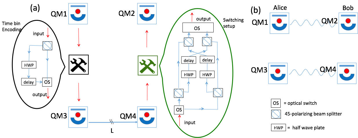
Figure 1: (a) Quantum multiplexing applied to the four qubits entanglement distribution scheme (Alice and Bob have two qubits each). A polarized photon is entangled with the electron spin states of an NV center to create the state $|g_{1}\left\rangle|D\left\rangle\right.+|e_{1}\left\rangle|A\left\rangle.\right.\right.\right.$ The polarization encoded information is then transferred to a time bin encoding on the photon through the "time bin encoding" converter. The photon interacts with the second NV center and travels across the channel to Bob. At Bob’s side, the photon interacts with an NV center followed by it passing through the "switching setup" operation which swaps the polarization and time bin degrees of freedom ($A_{\mathcal{S}}$ with the $D_{\mathcal{L}}$ mode). Finally, the photon interacts with the second NV center of Bob and is measured. Upon a successful measurement, the state of the four memories is projected into two maximally entangled states illustrated in (b).

In all the other cases no phase shift occurs. To illustrate this method, we assume that Alice and Bob, separated by a distance $L,$ have two NV centers each, as shown in Fig. 1(a), respectively. A $D-$ polarized photon interacts with the first NV center on Alice’s side giving Lo Piparo et al. (2017a)

$$|D\left\rangle|\psi_{1}\left\rangle{}_{in}\right.\right.\rightarrow|g_{1}\left\rangle|D\left\rangle\right.+|e_{1}\left\rangle|A\left\rangle,\right.\right.\right.$$ (1)

The next step (as shown in Fig. 1(a) is to transfer the information encoded into the polarization DOF into the time bin DOF through the "time bin encoding" converter. Our state is transformed to

$$|g_{1}\left\rangle|D_{\mathcal{S}}\left\rangle\right.+|e_{1}\left\rangle|D_{\mathcal{L}}\left\rangle,\right.\right.\right.$$ (2)

where the subscripts $\mathcal{S}$ and $\mathcal{L}$ indicate the short and long time-bins, respectively. The photon then interacts with the second NV center of Alice (labelled QM3), giving:

$$\begin{array}[]{c}\begin{array}[]{c}|g_{1}\left\rangle|g_{3}\left\rangle\right.|D_{\mathcal{S}}\left\rangle\right.+|g_{1}\left\rangle|e_{3}\left\rangle\right.|A_{\mathcal{S}}\left\rangle\right.\right.\right.\end{array}\\ \;\;\;\;\;\;\;\;\;+|e_{1}\left\rangle|g_{3}\left\rangle\right.|D_{\mathcal{L}}\left\rangle+\right.\right.|e_{1}\left\rangle|e_{3}\left\rangle\right.|A_{\mathcal{L}}\left\rangle.\right.\right.\end{array}$$ (3)

The photon then travels through the optical fiber, where, upon a successful transmission, it interacts with Bob’s first qubit (labelled QM4). While the photon’s transmission through the channel has a probabilistic nature, its success can be heralded by Bob eventual measurement of it. The probability of the photon arriving at Bob’s side is $P_{0}=e^{-L/L_{\mathrm{att}}},$ where $L_{\mathrm{att}}=25$ km is the attenuation length of the channel with $c$ being that speed of light in that channel. Now after this interaction with QM4 the photons degrees of freedom (polarization and timebin) are swapped with each other (the $D_{\mathcal{L}}$ component is switched with the $A_{\mathcal{S}}$ component). Then the photon interacts with the last NV center (labelled QM2) resulting in the state (conditioned on there being a photon at Bob’s side):

$$\begin{array}[]{c}\left.|\phi_{12}^{+}\right\rangle\left.|\phi_{34}^{+}\right\rangle\left.|D_{\mathcal{S}}\right\rangle+\left.|\psi_{12}^{+}\right\rangle\left.|\phi_{34}^{+}\right\rangle\left.|A_{\mathcal{S}}\right\rangle\\ \;\;\;\;\;\;\;\;\;\left.+|\phi_{12}^{+}\right\rangle\left.|\psi_{34}^{+}\right\rangle\left.|D_{\mathcal{L}}\right\rangle+\left.|\psi_{12}^{+}\right\rangle\left.|\psi_{34}^{+}\right\rangle\left.|A_{\mathcal{L}}\right\rangle\end{array}$$ (4)

where $\left.|\phi_{ij}^{+}\right\rangle=\left(\left.|g_{i}\right\rangle\left.|g_{j}\right\rangle+\left.|e_{i}\right\rangle\left.|e_{j}\right\rangle\right)$ and $\left.|\psi_{ij}^{+}\right\rangle=\left(\left.|g_{i}\right\rangle\left.|e_{j}\right\rangle+\left.|e_{i}\right\rangle\left.|g_{j}\right\rangle\right)$, for $i=1(3),$ $j=2(4).$ Bob will then measure the photon (both polarization and time bin’s DOF) and so heralds its successful transmission. The state of Eq. (4) will collapse in one of the four tensor products of entangled states under ideal conditions. Depending on the photons measurement result, bitflip operations can be performed on Bob qubits ensuring that Alice and Bob share the required state $\left.|\phi_{12}^{+}\right\rangle\left.|\phi_{34}^{+}\right\rangle$. Appendix D shows the situation with channel loss with more detail.

II.2 Advantages of the QMUXING entangling scheme

The main advantage of the QMUXING entangling scheme is that we only need one single photon to create two entangled pairs as compared to the conventional schemes where at least two single photon sources are needed. This means that we reduce the waiting time for entangling both pairs. In fact, in the QMUXING scheme the time to entangle that two pairs of memories is given by $2L/c,$ where $2L/c$ is simply the time for Alice to send her photon to Bob and Bob to return a success/failure message. In the case of success Alice and Bob can now use the entangled pairs whereas in the case of failure, Bob needs to send a message to Alice indicating another attempt is required including reinitializing of the quantum memories. The reduced waiting time for the QMUXING scheme means the quantum memories will dephase less and so will result in higher fidelity pairs being generated. It is straightforward to show that each pair of Fig. 1(b) will dephase simultaneously as

$$\rho_{ij}^{\mathrm{dph}}(F_{ij})=F_{ij}|\phi_{ij}^{+}\left\rangle\negmedspace\right.\left.\negmedspace\right\langle\phi_{ij}^{+}|+(1-F_{ij})Z_{ij}|\phi_{ij}^{+}\left\rangle\negmedspace\right.\left.\negmedspace\right\langle\phi_{ij}^{+}|Z_{ij}$$ (5)

with $Z_{ij}$ being the $Z$ Pauli operator while $F_{ij}=F=\left(1+e^{-\frac{3L}{cT_{2}}}\right)/2$ is the fidelity of the generated entangled state. In the latter fidelity expression, the term $3L/c$ takes into account the NV centers dephasing time for the photon to traveling from Alice to Bob and the heralding of a successful photon transmission to be communicated back to Alice while $T_{2}$ is the coherence time of the memory. For the four QMUXING scheme the state of the two entangled pairs can be written as

$$\begin{array}[]{c}\rho_{1234}^{\mathrm{dph}}(F)=\rho_{12}^{\mathrm{dph}}(F)\otimes\rho_{34}^{\mathrm{dph}}(F).\end{array}$$ (6)

Now let us investigate the conventional entangling scheme Sangouard et al. (2011a) as it leads to a different dephasing process as the entangled states are created at different times. Once the first entangled pair is created one must wait until the second pair has been created before further operations can be attempted. If we assume that the first(second) entangled pair created is $\rho_{34},$ $\rho_{12,}$ respectively, then the dephasing operation gives $\rho_{34}^{\mathrm{dph}}(F_{34}^{{}^{\prime}}),$ $\rho_{12}^{\mathrm{dph}}(F_{12})$ with $F_{34}^{{}^{\prime}}=\left(1+e^{-\frac{L}{cT_{2}}-\frac{2L}{cP_{0}T_{2}}}\right)/2,$ while $F_{12}$ is given by the expression above. The overall state for both entangled pair is then $\begin{array}[]{c}\rho_{1234}^{\mathrm{dph}}(F,F^{{}^{\prime}})=\rho_{12}^{\mathrm{dph}}(F)\otimes\rho_{34}^{\mathrm{dph}}(F^{{}^{\prime}})\end{array}$.

Next the QMUXING entangling scheme is not restricted to 2 entangled pairs and can easily be extended to create $N$ entangled pairs of NV centers separated by a distance (of course there are practical limitations to this). In this case, a single photon will interact with all Alice’s qubits and then, after ideally travels across the channel, will interact with Bob’s qubits. In general, for creating $N$ entangled pairs separated by a distance $L$, we need to encode the photon into $N-1$ DOFs. The photon components will be coupled in such a way to create the final state given by the sum of tensor products of entangled pairs between Alice and Bob.

The advantages of using the QMUXING entangling scheme is further increased for entangling a larger number of pairs, since the number of photons is independent on the number of pairs, as in a conventional entangling scheme. These pairs can then be used in further quantum tasks.

III Application of quantum multiplexing to entanglement purification

Let us now describe the method for generating high fidelity entangled states. A general purification protocol consists of performing local operations on $m$ entangled qubits pairs in order to create $n<m$ pairs with a higher fidelity than the initial pairs. One of the well known protocols to generate high fidelity pairs is the Deutsch purification protocol Deutsch et al. (1996) where Alice and Bob share two copies of the Bell diagonal state

$$\rho=A\rho_{\psi^{+}}+B\rho_{\psi^{-}}+C\rho_{\phi^{+}}+(1-A-B-C)\rho_{\phi^{+}},$$ (7)

with $\rho_{\psi^{\pm},\phi^{\pm}}$ being the density matrices associated with the Bell states, $|\psi^{\pm}\left\rangle=|10\left\rangle\right.\pm|01\left\rangle,\right.\right.$ and $|\phi^{\pm}\left\rangle=|11\left\rangle\right.\pm|00\left\rangle\right.\right.$. The coefficients $A,$ $B,$ and $C$ are constrained to give positive real eigenvalues with $Tr\rho=1$. Alice and Bob begin their purification protocol by applying an $X$ rotation on both their qubits, followed by CNOT operations on both sides. Once these have been performed, the target qubits are measured in the computational basis and the result is communicated classically. If the protocol is successful, the fidelity of the resulting state will be higher. In order to increase even further the fidelity of the state, Alice and Bob can iterate this procedure on two pairs having the same fidelity until they share a high fidelity entangled state.

An alternative way of creating high fidelity entangled pairs relies on error correction protocols. A conventional three qubit error correction protocol works as follows. Alice and Bob create three entangled pair and perform CNOT operations between the control qubits and the target qubits. They measure the target qubits and communicate classically the results of the measurements to each other. Depending on the outcomes they apply a specific logic gate on their control qubits to get the desired Bell state.

III.1 The QMUXING entangling scheme applied to the Deutsch purification protocol

Let is now apply the QMUXING entangling scheme to the Deutsch purification protocol. We use the same procedure to create the entangled state of Eq. (4) but then perform a Hadamard operation on the qubits. In this case, upon a successful photon transmission, our resulting state has the form

$$\begin{array}[]{c}\left.|\varphi_{12}^{+}\right\rangle\left.|\varphi_{34}^{+}\right\rangle\left.|D_{\mathcal{S}}\right\rangle+\left.|\chi_{12}^{+}\right\rangle\left.|\varphi_{34}^{+}\right\rangle\left.|A_{\mathcal{S}}\right\rangle\\ \;\;\;\;\;\;\;\;\;\left.+|\varphi_{12}^{+}\right\rangle\left.|\chi_{34}^{+}\right\rangle\left.|D_{\mathcal{L}}\right\rangle+\left.|\chi_{12}^{+}\right\rangle\left.|\chi_{34}^{+}\right\rangle\left.|A_{\mathcal{L}}\right\rangle\end{array}$$ (8)

with $\left.|\varphi_{ij}^{+}\right\rangle=\left(\left.|+_{i}\right\rangle\left.|+_{j}\right\rangle+\left.|-_{i}\right\rangle\left.|-_{j}\right\rangle\right)$ and $\left.|\chi_{ij}^{+}\right\rangle=\left(\left.|+_{i}\right\rangle\left.|-_{j}\right\rangle+\left.|-_{i}\right\rangle\left.|+_{j}\right\rangle\right)$, where $(i,\,j)=(1,\,2),$ $(3,\,4),$ respectively. Bob will measure the photon and will flip his qubits depending on the photon outcome as described in Sec. II. Alice and Bob then will perform a CNOT operation between their respective qubits and will measure the target qubits. They will communicate the outcomes of the target qubits to each other and they will keep the entangled pair if the outcomes are the same, otherwise they will start the protocol again.

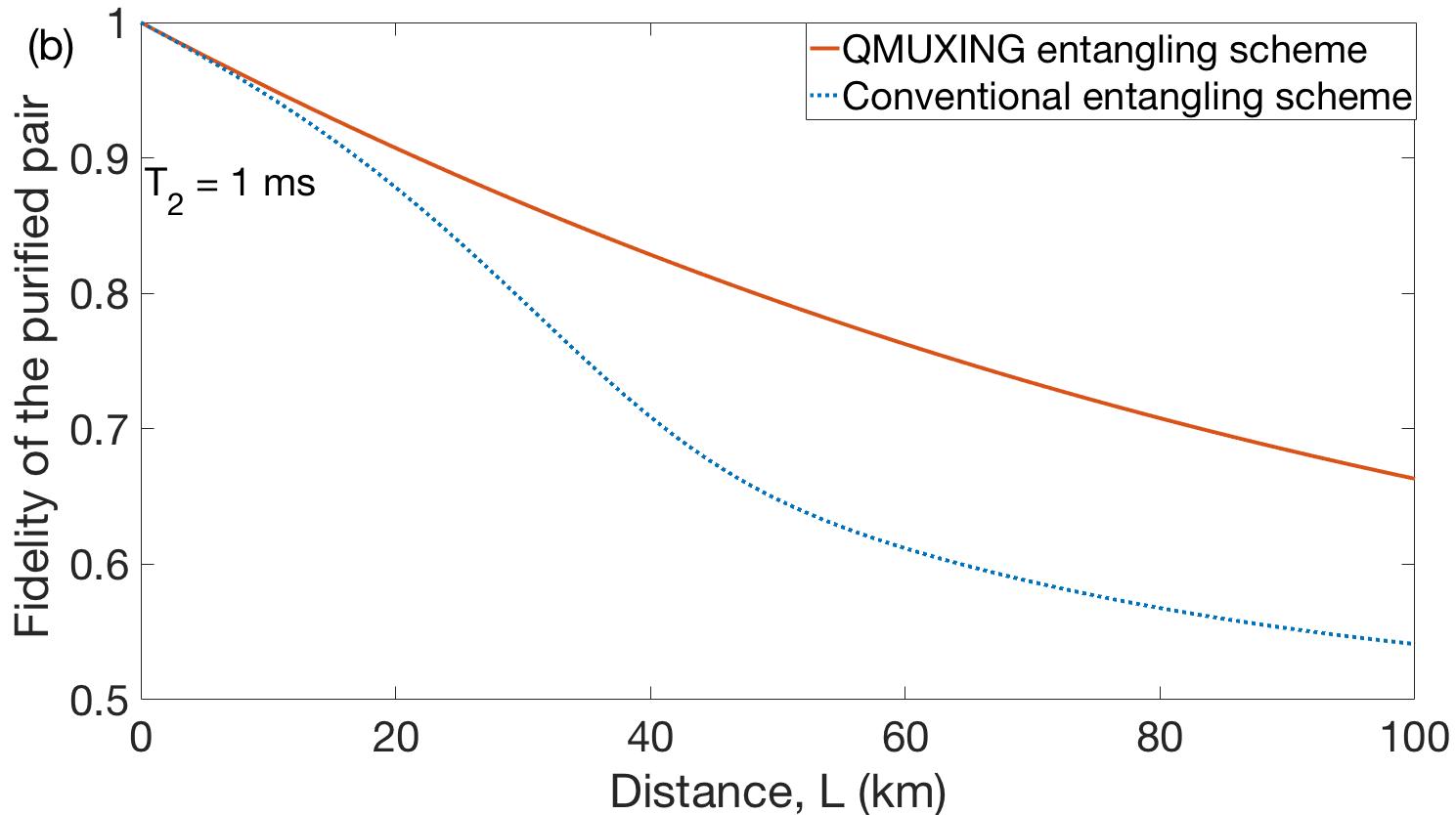
Figure 2: In (a), entanglement purification scheme of two entangled pairs and in (b) fidelities of the purified pair obtained through the Deutsch protocol in which the entangled pairs have been created with the QMUXING entangling scheme (solid lines) and with a traditional prepare and measure entangling scheme (dotted line) for a coherence time, $T_{2}=1$ ms.

Compared to the Deutsch purification scheme in which the quantum memories are created in the traditional way, our approach is faster due to the fact that both the entanglement creation and purification are acknowledged simultaneously. While the photon is transmitted through the channel both pairs will go through a dephasing quantum channel given by $\rho_{0}^{\mathrm{deph}}(F_{0})$ (see Eq. 5) where $F_{0}=$$\left(1+e^{-L/cT_{2}}\right)/2$. At this point a CNOT gate is applied and the target qubits are measured. The fidelity, $F_{\mathrm{QMX}},$ of the purified pair will be given by

$$F_{\mathrm{QMX}}=\frac{F_{0}^{2}}{F_{0}^{2}+(1-F_{0})^{2}}.$$ (9)

Now, Alice and Bob will communicate classically the outcomes of their measurement therefore their state, $\rho_{\mathrm{QMX}}^{\mathrm{dph}}$, will dephase to $\rho_{\mathrm{QMX}}^{\mathrm{dph}}(F_{\mathrm{QMX}}^{\mathrm{dph}}),$ where $F_{\mathrm{QMX}}^{\mathrm{dph}}=\left(1+(2F_{\mathrm{QMX}}-1)e^{-2L/cT_{2}}\right)/2$ (see Appendix E for details).

Now in the traditional Deutsch protocol where the entanglement distribution is done independently per pair the fidelity of the purified pair will be given by

$$F_{\mathrm{trad}}=\frac{F_{12}F_{34}^{{}^{\prime}}}{F_{12}F_{34}^{{}^{\prime}}+(1-F_{12})(1-F_{34}^{{}^{\prime}})},$$ (10)

where $F_{12}$ and $F_{34}^{{}^{\prime}}$ have been defined in Sec. II. After the entangled pairs are created, Alice and Bob will perform the local operations and will measure their target qubits. Then they will communicate the outcomes of the measurement to each other. During this time, the purified pair state, $\rho_{\mathrm{trad}}^{\mathrm{dph}},$ will dephase to $\rho_{\mathrm{trad}}^{\mathrm{dph}}(F_{\mathrm{trad}}^{\mathrm{dph}}),$ where $F_{\mathrm{trad}}^{\mathrm{dph}}=\left(1+(2F_{\mathrm{trad}}-1)e^{-2L/cT_{2}}\right)/2.$

Now in Figure 2(b) we compare $F_{\mathrm{QMX}}^{\mathrm{dph}}$ and $F_{\mathrm{trad}}^{\mathrm{dph}}$ versus $L$ where we have set a $T_{2}=1$ ms coherence time for the memories. We observe that for short distances the two fidelities are almost the same. However, at distances larger than $20$ km the fidelity of the entangled pair created by the QMUXING scheme is much higher compared to the one of the entangled pair created with the traditional entangling scheme. This advantage is biggest at $L=50$ km where $F_{\mathrm{QMX}}^{\mathrm{dph}}=0.8$ and $F_{\mathrm{trad}}=0.6.$

III.2 The QMUXING protocol

We illustrate here a method, which has been introduced in pri , to create high fidelity entangled pairs through the QMUXING entangling scheme with a built-in purification protocol. We call this method QMUXING protocol. A remarkable feature of encoding a photon into multiple DOFs is that the DOFs correspond to qubits on which we might perform the same local operations applied above. This in turn means the number of matter qubits can be reduced.

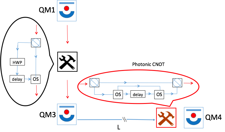
Figure 3: Three qubit quantum multiplexing protocol. The first two steps are identical as the ones described in Fig. 1. The spin states of the NV centers are rotated into the diagonal basis. When the photon being transmitted across the channel arrives at Bob a CNOT operation is performed between QM3 and QM1 and between the photonic modes of the photon through the “photonic CNOT” operation of the Figure. The photon then interacts with the last NV center and it is measured. The protocol is successful if Alice measures “$+(-)"$ and Bob will measures “$\mathcal{S}(\mathcal{L})"$ on the photons degree of freedom. In any other case, the protocol is aborted and Alice and Bob start again.

In this protocol, the state of our system, after the photon has been interacted with the memories QM1 and QM3 of Fig. 3, is given by Eq. (3). A Hadamard applied to Alice’s qubit gives:

$$|++D_{\mathcal{S}}\left\rangle+|+-A_{\mathcal{S}}\left\rangle+\right.|-+D_{\mathcal{L}}\left\rangle+\right.|--A_{\mathcal{L}}\left\rangle.\right.\right.$$ (11)

We can now apply a CNOT operation between QM3 (control) and QM1 (target) and between the polarization DOF (control) and the TB DOF (target). This CNOT operation works as follows: the diagonal component will leave unaffected the time-bin component and the antidiagonal component will flip the time-bin component. The CNOT on the photonic qubits can be implemented by the scheme represented in the the “photonic CNOT” operation of Fig. 3. Upon a successful transmission of the photon through the channel (which will be heralded by the photon measurement), the photon then interacts with QM4, which is successively rotated in the diagonal basis. The final resulting state has the form:

$$\begin{array}[]{c}\begin{array}[]{c}|+_{1}\left\rangle\negmedspace\right.|\varphi_{34}^{+}\left\rangle\negmedspace\right.|D_{\mathcal{S}}\left\rangle\negmedspace\right.+|+_{1}\left\rangle\negmedspace\right.|\chi_{34}^{+}\left\rangle\negmedspace\right.|A_{\mathcal{S}}\left\rangle\negmedspace\right.\end{array}\\ \;\;\;\;\;\;\;\;\;+|-_{1}\left\rangle\negmedspace\right.|\chi_{34}^{+}\left\rangle\negmedspace\right.|A_{\mathcal{L}}\left\rangle\negmedspace\right.+|-_{1}\left\rangle\negmedspace\right.|\varphi_{34}^{+}\left\rangle\negmedspace\right.|D_{\mathcal{L}}\left\rangle\negmedspace\right.\end{array}$$ (12)

Alice with now measure QM1 in the diagonal basis while at the same time Bob measures the state of the photon (both degrees of freedom). They communicate the results with each other via the classical communications channel. A purified pair is obtained if the outcomes of QM1 is “$+(-)"$ and of the TB DOF is “$\mathcal{S}(\mathcal{L})",$ respectively. In this case the states will be given by $|\varphi_{34}^{+}\left\rangle,\right.$ $|\chi_{34}^{+}\left\rangle\right.$ respectively. For the “$+\mathcal{L}"$ and “$-\mathcal{S}"$ results the protocol has failed and we need to begin again with the entanglement distribution. Of course this considerations have not included dephasing yet. It can be simply handled (appendix F) and for instance with the ($+$, $\mathcal{S}$) measurement result, our quantum state would have the form

$$\begin{array}[]{c}\negthickspace\negthickspace\negthickspace\rho_{\mathrm{3}}=\frac{F^{2}}{F^{2}+(1-F)^{2}}|\varphi_{34}^{+}\left\rangle\negmedspace\right.\left.\negmedspace\right\langle\varphi_{34}^{+}|+\frac{(1-F)^{2}}{F^{2}+(1-F)^{2}}X_{3}|\varphi_{34}^{+}\left\rangle\negmedspace\right.\left.\negmedspace\right\langle\varphi_{34}^{+}|X_{3},\end{array}$$ (13)

where $X_{3}$ is the $X$ Pauli operator applied to QM3.

We can also generalize the QMUXING protocol to a larger number of memories. In this case, if $N$ is the total number of pairs of a conventional protocol, the total number of matter qubits that we need QMUXING protocol will be given by $N+1,$ since we need $N-1$ effective extra DOFs are needed to entangled $N$ pairs (this can be also ex TB modes).

We can further reduce the number of matter qubits if we use the nuclear spin of an NV center as a qubit. We can in fact transfer the electron spin state of the NV center into the nuclear spin after the first interaction of the photon. In this way, the photon can interact again with the electron spin and then travel across the channel where it will interact with Bob’s qubit (see Appendix G).

IV Performance metrics

It is important now to investigate quantitatively what improvements this new scheme gives. As the main figure of merit, we will calculate the rate at which Alice and Bob can share purified entangled states normalized by the number of physical resources (the number of matter qubits or quantum memories and the average number of single photons needed to create the entangled states). In order to evaluate the impact of the number of resources used, we introduce the cost functions $C_{M}$ and $C_{p},$ which multiply the number of matter qubits and the average number of single photons, respectively.

IV.1 Normalized purification rates

For a purification protocol with $k$ purification rounds our normalized rate is defined by:

$$R_{\alpha}(k)=\frac{r_{\alpha}(k)}{M_{\alpha}(k)C_{M}+m_{\alpha}(k)C_{p}},$$ (14)

where $r_{\alpha}(k)$ is the raw rate for establishing a high fidelity entangled pair over a distance $L$ and with the subscript $\alpha=\mathrm{QMX}$ ($\alpha=\mathrm{D}$) referring to the QMUXING protocol (Deutsch protocol with traditional entanglement creation), respectively. The rate of establishing purified pairs after $k$ purification rounds using the QMUXING protocol is given by $R_{\mathrm{QMX}}(k)$ with

$$\left(r_{\mathrm{QMX}}(k)\right)^{-1}=\frac{2}{c}\frac{L}{P_{0}\prod_{I=1}^{k}P_{D}(i)},$$ (15)

where $P_{D}$ is the probability of a successful purification round with $M_{\mathrm{QMX}}(k)=2^{k}+1$ and $m_{\mathrm{QMX}}(k)=1/P_{0}.$ The rate $r_{\mathrm{QMX}}(k)$ is given by only one term associated with the time the photon travels on the optical fiber and reach Bob side and the time for classical communication. The number of matter qubits is less than the traditional purification scheme due to the local operations performed on the extra DOFs of the photon. Similarly the rate, $R_{\mathrm{D}},$ of the Deutsch protocol for a fixed number, $k,$ of distillation rounds which entangle pairs generated conventionally is given by $R_{D}(k)$ with

$$\begin{array}[]{c}\left(r_{\mathrm{D}}(k)\right)^{-1}=\left(\frac{3}{2}\right)^{k}\frac{2}{c}\frac{L}{P_{0}\prod_{I=1}^{k}P_{D}(i)}\\ +\left(\frac{3}{2}\right)^{k-1}\frac{L}{c\prod_{I=1}^{k}P_{D}(i)}+...\frac{L}{cP_{D}(1)},\end{array}$$ (16)

where $M_{\mathrm{D}}(k)=2^{k+1}$ and $m_{\mathrm{D}}(k)=2^{k}/P_{0}$. The first term is the rate to establish an entangled state over a distance $L$ and to communicate classically that the entangling step has been successful. The factor $3/2,$ is the average waiting time to prepare two entangled pairs. The other terms are associated with the times to acknowledge that the $k-$th distillation rounds has occurred. These latter terms are not present in the rate of our QMUXING protocol as the purification steps are performed during the time to establish the entanglement.

Next to quantify the improvement we have, let us calculate the ratio of the rates, $R_{\mathrm{QMX}}/R_{\mathrm{D}},$ for $k=1$ and $k=2,$ respectively. In order to analyze the effect of the number of the physical resources, we vary the weighting coefficients $\frac{}{}C_{M}$ and $C_{p}.$

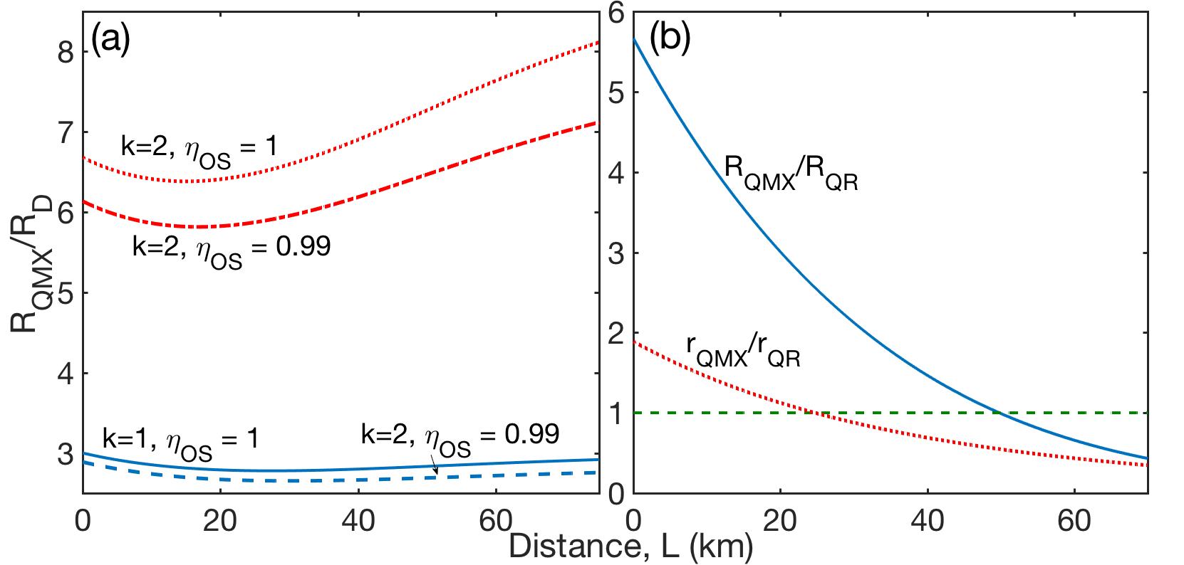
Figure 4: Ratio (a) between the normalized rates of the QMUXING protocol and the Deutsch protocol for one and two distillation rounds with perfect (dotted line and solid line, respectively) and imperfect (dash-dotted line and dashed line, respectively) optical switches, respectively and (b) between the three qubit QMUXING protocol and a conventional single node quantum repeater scheme. In (b), the intersections of the curves with the green dashed line show the crossover distances. We modeled the imperfection of the optical switches as a loss even with transmission probability $\eta_{OS}=0.99.$

In Fig. 4(a) we plot $R_{\mathrm{QMX}}/R_{\mathrm{D}}$ versus the distance for $k=1$ and $k=2$ in the ideal case of perfect optical switches. The two curves show an average increment of the rate equal to $2.5$ and 7 for a total distance of $L=70$ km, respectively, compared to $R_{D}$. They both have a minimum value at $L=25$ km and $L=15$ km, respectively. In fact, if we consider the rates for the case of $k=1,$ for $C_{M}=C_{p}=1,$ this ratio can be expressed as:

$$\frac{R_{\mathrm{QMX}}}{R_{\mathrm{D}}}=\frac{r_{\mathrm{QMX}}}{r_{\mathrm{D}}}\frac{4P_{0}+2}{3P_{0}+1}=\left(\frac{3}{2}+\frac{P_{0}}{2}\right)\frac{4P_{0}+2}{3P_{0}+1}.$$ (17)

This shows that the improvement of our protocol is then given by two factors: the increment of the rate of establishing an entangled state, which depend on the factor $3/2$ and on the distance between the users. Additionally, the latter term is multiplied by the ratio between the number of resources, which are less in our protocol. The ratio between the raw rates decreases exponentially with the distance as well as the ratio between the number of resources increases exponentially with the distance. Therefore, we expect a minimum increment in the ratio at certain distance. The $k=2$ case follows a similar explanation. Figure 4(a) shows also the case in which the optical switches efficiency is 0.99. As expected for $k=2$ the difference between the two curves is higher than the one for $k=1$ due to the higher number of optical switches needed.

We can also compare the rate of the three-qubit QMUXING protocol with the rate of a single node quantum repeater protocol in which the pairs has been purified at a distance $L_{0}=L/2.$ For such a system the rate of creating a purified pair over a distance $L$ is given by $R_{\mathrm{QR}}=r_{\mathrm{QR}}/(8C_{M}+4C_{p}/P_{0}^{1/2}$) with

$$(r_{\mathrm{QR}})^{-1}=\left(\frac{3}{2}\right)^{2}\frac{2}{c}\frac{L/2}{P_{0}^{1/2}P_{D}P_{ES}}+\frac{3}{2}\frac{L/2}{cP_{D}P_{ES}}+\frac{L/2}{cP_{ES}},$$ (18)

where $P_{ES}$ is the probability of a successful entangling swapping operation (assumed to be 0.9 here). Figure 4(b) shows the ratio of both the normalized rate and the raw rate of the QMUXING protocol against the standard one node quantum repeater protocol, in which the pairs have been purified over a distance $L/2.$ The normalized(raw) rate of the QMUXING protocol outperforms the one of the single node QR up to a distance $L\sim 50$(25) km (see Fig. 4(b). We can also apply the QMUXING protocol to a single node QR scheme. In this case, our rate outperforms the conventional one for all distances.

IV.2 Normalized rate in the error correction scheme

For an $N$-qubits error correction protocol the normalized rate is similarly given by:

$$R_{\alpha}^{\mathrm{EC}}(N)=\frac{r_{\alpha}^{\mathrm{EC}}(N)}{M_{\alpha}(N)C_{M}+m_{\alpha}(N)C_{p}},$$ (19)

where $r_{\alpha}^{\mathrm{EC}}(N)$ is the raw rate for creating a high fidelity pair. The rate of the three-qubit error correction QMUXING protocol is given by $R_{\mathrm{QMX}}^{\mathrm{EC}}$ with $\begin{array}[]{c}\left(r_{Q\mathrm{MX}}^{E\mathrm{C}}\right)^{-1}=\frac{2}{c}\frac{L}{P_{0}},\end{array}$ $M_{\mathrm{QMX}}(3)=4$ and $m_{\mathrm{QMX}}(3)=1/P_{0}.$ The rate of the three-qubit error correction protocol in which the pairs are created in the conventional way is given by $R_{\mathrm{D}}^{\mathrm{EC}}$ with $r_{\mathrm{D}}^{\mathrm{EC}}=1.7\frac{2}{c}\frac{L}{P_{0}}$ and $m_{\mathrm{D}}(3)=3/P_{0}$. The factor $1.7/P_{0}$ is an approximative value for the average time we have to wait in order entangle three pairs (Appendix A).

In Fig. 5 we plot $R_{\mathrm{QMX}}^{\mathrm{EC}}/R_{\mathrm{D}}^{\mathrm{EC}}$. In this case, the ratio between the raw rates is constant as shown in Fig. 5 and it increases with the distance reaching a value of $5$ at $L=70$ km. By considering imperfect optical switches this ration is a bit lower as shown in the dashed line of Fig. 5.

Since it is not straightforward to estimate the actual values of $C_{M}$ and $C_{p},$ we calculate the ratio of the normalized rates at a fixed distance versus the ratio of the cost functions $C_{M}$ and $C_{p},$ as illustrated in Fig. (6). The point $C_{M}=C_{p}=1,$ which correspond to the case of Fig. (4), splits the $x-$axis into two parts. For $C_{M}<C_{p}$ the normalized rate of our protocol achieves higher values compared to the case of equal cost function. That means that when we include the number of physical resources in the purification protocol, it is more convenient using a less number of matter qubits than the average number of single photons. The cost functions $C_{M}$ and $C_{p}$ might depends on several factors, such as its effective commercial costs and other characteristics.

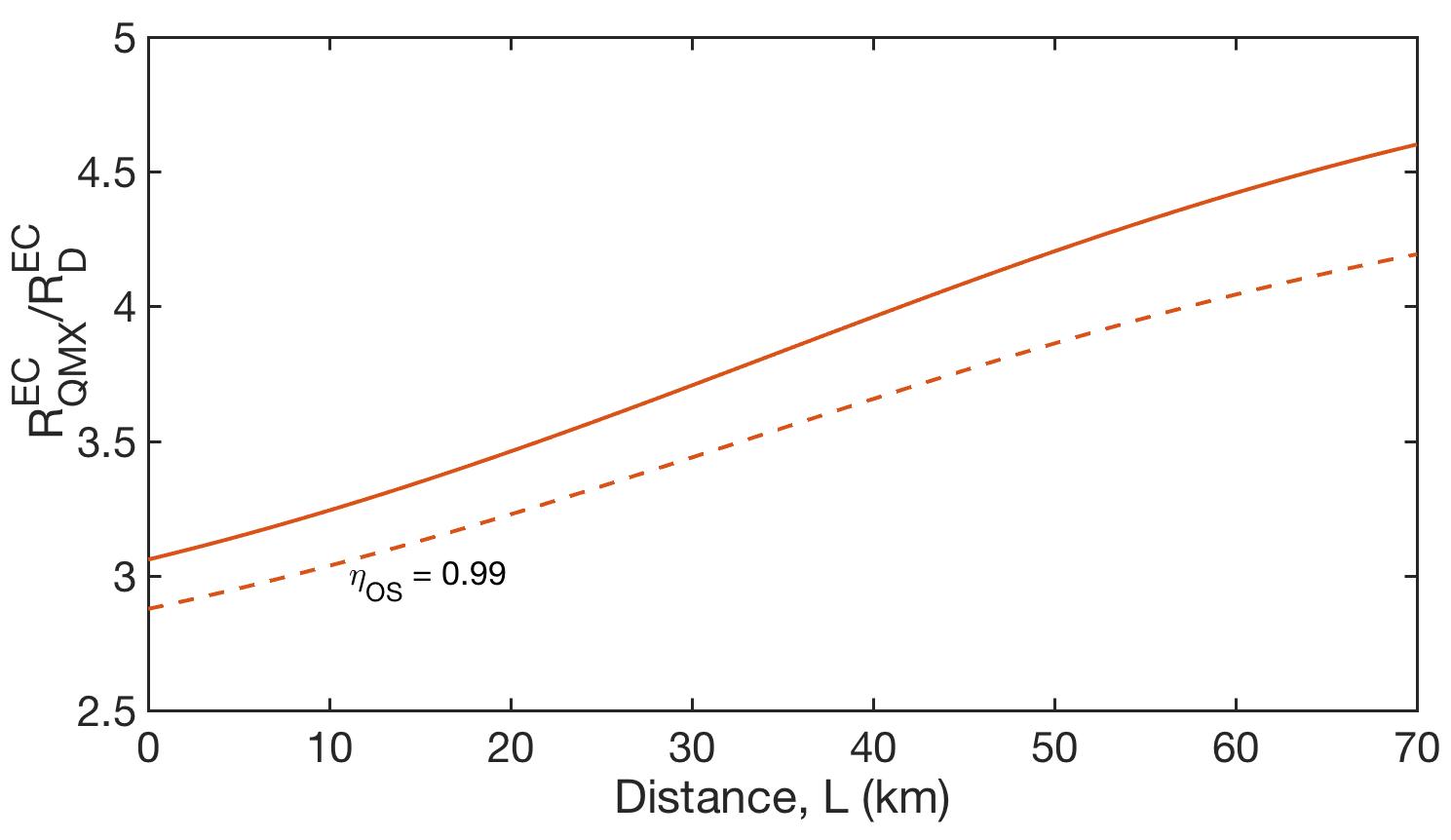
Figure 5: Ratio between the rate of the 3-qubit QMUXING protocol with built-in error correction protocol and the rate of the 3-qubit error correction protocol in which the pairs are created in the conventional way perfect (solid line) and imperfect optical switches (dashed line).

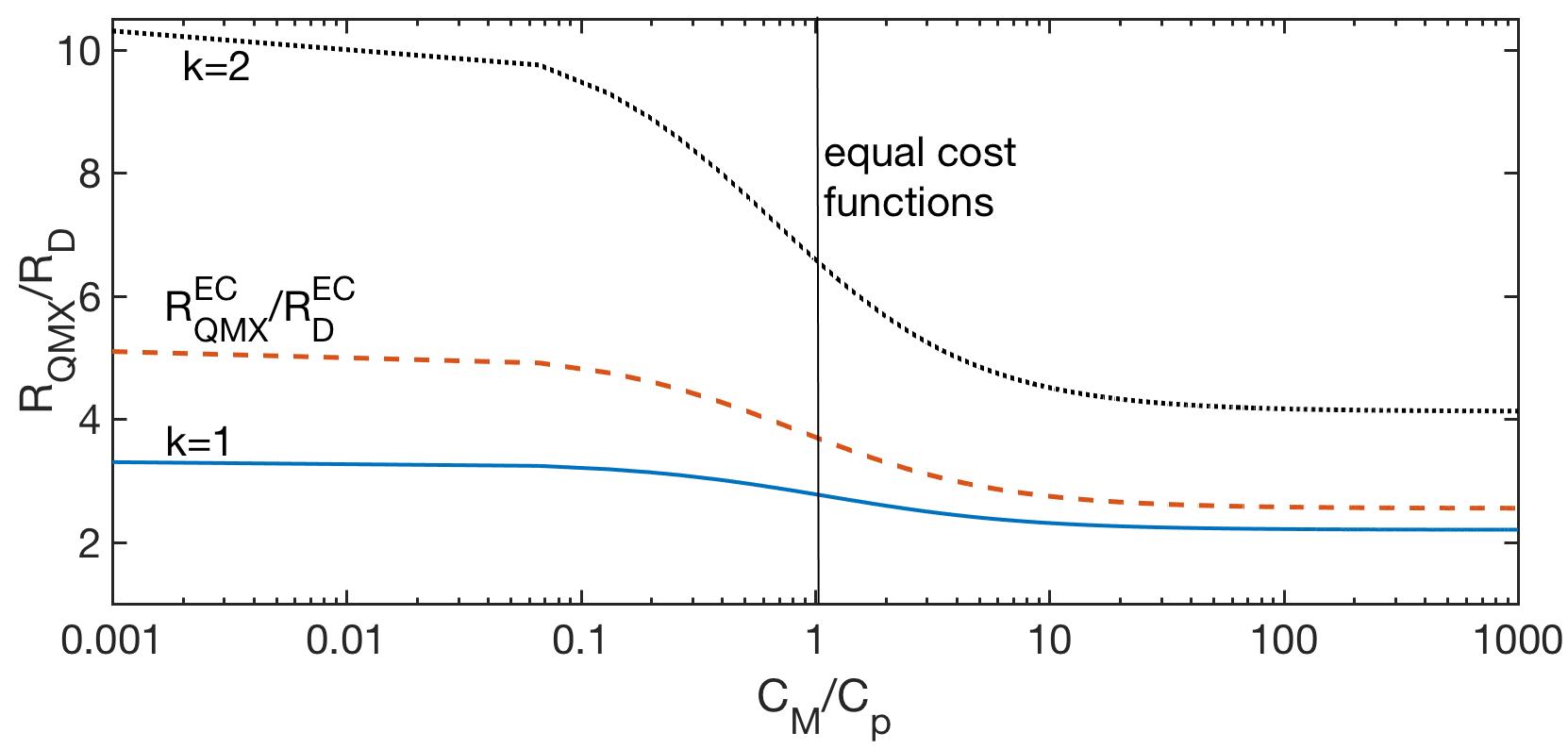
Figure 6: Ratio between the cost functions $C_{M}$ and $C_{p}$ at a distance $L=30$ km. The vertical line corresponds to the case when $C_{M}=C_{p}.$ At a fixed distance between Alice and Bob, higher (lower) values of $C_{p}$ respect to $C_{M}$ correspond to a bigger(smaller) increment of the ratio of the two rates.

V Discussion and Conclusion

In this work, we have introduced a new entangling scheme that allows to create multiple entangled pairs by using only a single photon. The photon, encoded in multiple degrees of freedom (DOFs), will entangle a series of NV centers prepared locally through the scheme Lo Piparo et al. (2017a). By switching among the various degrees of freedom entangled pairs between two remote users can be created. We call this new entangling method “quantum multiplexing” (QMUXING), since the photon carries multiple DOFs. The advantage of using such a method is the less number of resources needed and the lower average waiting time for creating an entangled pair. This will reduce the detrimental effects of the decoherence effect on the quantum memories in use.

We have also applied the quantum multiplexing method to the Deutsch purification protocol and shown that the raw generation rate is faster in our case compared to the conventional entangling scheme. We also use the QMUXING entangling scheme to generate purified entangled pairs with a built-in purification protocol on which the extra qubits of the photon are used as effective qubits. In this way, for a given number of purification rounds, $k,$ of a purification protocol in which the entangled pairs have been created with a conventional entangling scheme, we reduce the number of matter qubits when the QMUXING protocol is in use. In order to estimate the rate at which Alice and Bob can share a purified entangled pair after $k$ distillation rounds, we use a normalized figure of merit that takes into account the raw entanglement rate over the total number of physical resources, in terms of matter qubits and average number of single photons. To each of these parameters we associate a cost function in order to assess the impact of such resources on the rate. We plot the ratio of the normalized rate of our new protocol and the rate of creating high fidelity pairs through the Deutsch protocol for $k=1$ and $k=2$ and for the three-qubit error correction protocol when the entangled pairs are created with a traditional method and when perfect optical switches are in use. Initially, we consider that the cost functions are equal. We obtain that our protocol is roughly 2.5 faster than the other purification system for $k=1$ and up to $7$ times faster for $k=2.$ The QMUXING with error correction built-in scheme is 4.5 times faster than the conventional error correction protocol. For such a system, we calculate the average waiting time of entangling three pairs and we extend this calculation also for a number of pairs until $10.$ These values of the average time can be used in a further work in order to estimate the difference between the rate of a purification protocol having $N$ entangled pairs and an error correction protocol with the same number of qubits. We then calculate the ratio of the rate of the QMUXING protocol and the rate of Deutsch protocol with pairs created with a traditional scheme versus the ratio of the cost functions related to the matter qubits, $C_{M},$ and to the average number of photons, $C_{p},$ at a fixed distance. We find that our protocol shows a bigger improvement when the photon cost is more expensive than the memories.

Our QMUXING entangling scheme can also be applied to other quantum communication protocols, such as a the multiple memories configuration in a quantum repeater protocol, and to any protocol that requires entanglement distribution between two remote users. Moreover, the lower number of physical resources needed can dramatically reduce the costs required for its implementation.

Appendix A Entanglement distribution time for multiple pairs

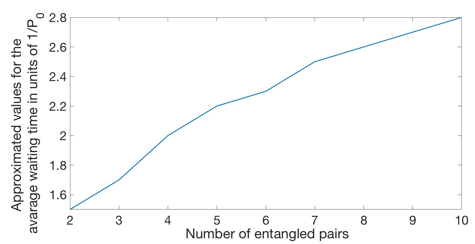
Figure 7: Approximative values in units of $1/P_{0}$ of the average waiting time for entangling $N=2$ to $N=10$ pairs separated by a distance $L$.

Let us now derive the average waiting probability of establishing three entangled pairs. We used this value for estimate the rate of a the three-qubit error correction protocol described in Sec. IVB.

Given a success entanglement probability $P_{0},$ the distribution probability of the number of attempts, $n,$ before we can establish an entangled pair over an elementary link is given by Sangouard et al. (2011b):

$$p(n)=(1-P_{0})^{n-1}P_{0}.$$ (20)

The distribution probability for entangling three elementary links will be given by:

$$\negthickspace q(n)=p(n)^{3}+3p(n)^{2}\sum_{k=1}^{n-1}p(k)+3p(n)\sum_{r=1}^{n-1}p(k)\sum_{s=1}^{n-1}p(k).$$ (21)

whose expectation value is given by:

$$\left\langle n\right\rangle=\sum_{n=0}^{\infty}nq(n)=\frac{3P_{0}^{3}-12P_{0}^{2}+19P_{0}-11}{P_{0}(P_{0}^{2}-3P_{0}+3)(P_{0}-2)}.$$ (22)

For small $P_{0},$ the expression in Eq. 22 can be approximated by $\left\langle n\right\rangle\sim 1.7/P_{0}$. In addition to that, in the prepare and measure entangling scheme, the average waiting time for entangling $N$ pairs will increase, as shown in Fig. 7 for $N=3..10.$ By applying the QMUXING entangling scheme on the other hand, if we neglect the interaction time of the photon with the quantum memory, the average waiting time for entangling $N$ pairs will still be proportional to $L/cP_{0}$ (we have not included the communication time).

Appendix B Optical switch error model

In a real implementation of the QMUXING entangling scheme, we have to consider the errors associated with the optical switches, since they are the only new optical elements which are not present in the conventional entangling scheme. We model this error as a loss of the photon, with transmission coefficient given by $\eta_{OS}.$ We both consider the ideal case, in which $\eta_{OS}=1,$ and the more realistic case, in which $\eta_{OS}=0.99$. The number of times the optical switches are used in the quantum multiplexing scheme depends on the number of pairs $N$ we want to entangle. In particular, for each pair creation we have to add a time-bin component by using the gates of the black bubble of Fig. 1 and then, after the photon has travelled across the channel, we have to perform the operations of the green bubble of Fig. 1 for each pair we want to entangle. Therefore, for $N$ entangled pairs we want to create, the number of optical switches is given by $\frac{3}{2}N-3.$ Therefore, we substitute $P_{0}$ with $P_{0}^{{}^{\prime}}=\eta_{OS}^{\frac{3}{2}N-3}P_{0}.$

Appendix C QMUXING entangling scheme with channel loss

The state of our system after the photon has interacted with Alice’s NV centers is given by Eq. (3). Now we assume that the photon travels across the channel and reaches Bob’s side with probability $P_{0}$ and it is lost with probability $1-P_{0}.$ Therefore, the final state will be described by the following density matrix:

$$\begin{array}[]{c}\rho_{tot}=P_{0}\rho_{1234}+(1-P_{0})(I_{13}\otimes\rho_{24}),\end{array}$$ (23)

where $\rho_{1234}=|\psi_{1234}\left\rangle\left\langle\psi_{1234}|\right.\right.$ is the density matrix of the state of Eq. (4), $I_{13}$ is the complete mixed state of the subspace spanned by the base vectors $g_{1},$ $g_{3},$ $e_{1},$ and $e_{3}.$ $\rho_{24}=|\varphi_{24}\left\rangle\left\langle\varphi_{24}|\right.\right.$, where $|\varphi_{24}\left\rangle=\left(|g_{2}\left\rangle+|e_{2}\left\rangle\right.\right.\right)\left(|g_{4}\left\rangle+|e_{4}\left\rangle\right.\right.\right)|0\left\rangle{}_{p}\right.\right.$ with $|0\left\rangle{}_{p}\right.$ the vacuum term of the photonic mode.

Appendix D Dephasing model in the four qubits QMUXING entangling scheme applied to the Deutsch protocol

Let us consider the situation where the quantum memories dephase over time. The lost in fidelity during this time is $1-F$. For the sake of simplicity we assume that Bob will measure a $D_{\mathcal{S}}$ photon (all the other cases can be obtained by flipping Bob’s qubits). A dephasing channel applied to the state of Eq. (8) will produce the state.

$$\begin{array}[]{c}\rho_{\mathrm{4}}=F^{2}\rho_{0}+F(1-F)(X_{1}\rho_{0}X_{1}+X_{3}\rho_{0}X_{3})\\ +(1-F)^{2}X_{1}X_{3}\rho_{0}X_{1}X_{3},\end{array}$$ (24)

where $\rho_{0}=|\psi_{0}\left\rangle\left\langle\psi_{0}|,\right.\right.$ and $|\psi_{0}\left\rangle=|\varphi_{12}^{+}\left\rangle|\varphi_{34}^{+}\left\rangle\right.\right.\right.$. By following the Deutsch protocol Alice and Bob apply a CNOT gate between QM3(QM4) and QM1(QM2), respectively. The resulting state will be

$$\begin{array}[]{c}\negthickspace\negthickspace\negthickspace\rho_{\mathrm{4}}=F^{2}\rho_{0}+F(1-F)(X_{1}\rho_{0}X_{1}+X_{1}X_{3}\rho_{0}X_{1}X_{3})\\ +(1-F)^{2}X_{3}\rho_{0}X_{3},\end{array}$$ (25)

Alice and Bob will measure their target qubits and they communicate to each other the outcomes. The protocol is successful when the outcomes are the same. If, for instance, the outcome are both $"+"$ the final state will be given by

$$\begin{array}[]{c}\rho_{\mathrm{4}}^{{}^{\prime}}=\frac{F^{2}}{F^{2}+(1-F)^{2}}|\varphi_{34}^{+}\left\rangle\left\langle\varphi_{34}^{+}|\right.\right.\\ +\frac{(1-F)^{2}}{F^{2}+(1-F)^{2}}X_{3}|\varphi_{34}^{+}\left\rangle\left\langle\varphi_{34}^{+}|X_{3}.\right.\right.\end{array}$$ (26)

References

- Feynman (1982) R. P. Feynman, International Journal of Theoretical Physics 21, 4467 (1982).
- Simon (1994) D. R. Simon, Foundations of Computer Science, 1994 Proceedings., 35th Annual Symposium on , 116 (1994).
- DiVincenzo (1995) D. P. DiVincenzo, Science 270, 255 (1995).
- Dowling and Milburn (2003) J. P. Dowling and G. J. Milburn, Phil. Trans. R. Soc. A 361, 3655 (2003).
- Dogen et al. (2017) C. L. Dogen, F. Reinhard, and P. Cappellaro, Rev. Mod. Phys. 89, 035002 (2017).
- Simon et al. (2014) D. S. Simon, G. Jaeger, and A. V. Sergienko, Int. J. Quantum Inform. 12, 1430004 (2014).
- Lugiato et al. (2002) L. A. Lugiato, A. gatti, and E. Brambilla, J. Opt. B 4, 176 (2002).
- Bennett and Brassard (2014) C. H. Bennett and G. Brassard, Theoretical computer science 560, 7 (2014).
- Sangouard et al. (2011a) N. Sangouard, C. Simon, C. De Riedmatten, and N. Gisin, Rev. Mod. Phys. 83, 33 (2011a).
- Ekert (1991a) A. K. Ekert, Phys. Rev. Lett. 67, 661 (1991a).
- Lo (1999) H. Lo, Science 283, 2050 (1999).
- Hwang (2003) W.-Y. Hwang, Phys. Rev. Lett. 91, 057901 (2003).
- Munro et al. (2015) W. J. Munro, K. Azuma, K. Tamaki, and K. Nemoto, IEEE Journal of Selected Topics in Quantum Electronics 21, 6400813 (2015).
- Nielsen and Chuang (2000) M. Nielsen and I. Chuang, Quantum Computation and Quantum Information (Cambridge University Press, Cambridge, 2000).
- Bennett and DiVincenzo (2000) C. Bennett and D. DiVincenzo, Nature 404, 247 (2000).
- Raussendorf and Briegel (2001) R. Raussendorf and H. J. Briegel, Phys. Rev. Lett. 86, 5188 (2001).
- Knill (2005a) E. Knill, Nature 434, 39 (2005a).
- Duan and Raussendorf (2005) L.-M. Duan and R. Raussendorf, Phys. Rev. Lett. 95, 080503 (2005).
- Devitt et al. (2013a) S. J. Devitt, A. M. Stephens, W. J. Munro, and K. Nemoto, Nature Communications 4, 2524 (2013a).
- Ekert (1991b) A. Ekert, Phys. Rev. Lett. 67, 661 (1991b).
- Bennett (1992) C. Bennett, Science 257, 752 (1992).
- Jennewein et al. (2000) T. Jennewein, C. Simon, G. Weihs, H. Weinfurter, and A. Zeilinger, Phys. Rev. Lett. 84, 4729 (2000).
- Long and Liu (2002) G. Long and X. Liu, Phys. Rev. A 65, 032302 (2002).
- Bennett et al. (1996a) C. Bennett, G. Brassard, S. Popesco, B. Schumacher, J. Smolin, and W. Wootters, Phys. Rev. Lett. 76, 722 (1996a).
- Deng et al. (2005) F. Deng, C. Li, Y. Li, H. Zhou, and Y. Wang, Phys. Rev. A 72, 022338 (2005).
- Barrett et al. (2004) M. D. Barrett, J. Chiaverini, T. Schaetz, J. Britton, W. M. Itano, J. D. Jost, E. Knill, C. Langer, D. Leibfried, R. Ozeri, and D. J. Wineland, Nature 429, 737 (2004).
- Ma et al. (2012) X.-S. Ma, T. Herbst, T. Scheidl, D. Wang, S. Kropatschenk, W. Naylor, B. Wittmann, A. Mech, J. Kofler, E. Anisimova, V. Marakov, T. Jennewein, T. Ursin, and A. Zeilinger, Nature 489, 269 (2012).
- Takesue et al. (2015) H. Takesue, S. D. Dyer, J. S. Martin, V. Verma, R. P. Mirin, and S. W. Nam, Optica 2, 832 (2015).
- Horodecki et al. (2007) R. Horodecki, P. Horodecki, M. Horodecki, and K. Horodecki, Rev. Mod. Phys. 81, 865 (2007).
- Mattle et al. (1996) K. Mattle, H. Weinfurter, P. G. Kwiat, and A. Zeilinger, Phys. Rev. Lett. 76, 4656 (1996).
- Kwiat et al. (1996) P. G. Kwiat, K. Mattle, H. Weinfurter, and A. Zeilinger, Optics and Photonics News 7, 14 (1996).
- (32) G. Vittorini, D. Hucul, V. Inlek, C. Crocker, and C. Monroe, Phys. Rev. A .
- Chou et al. (2005) C. Chou, R. de Riedmatten, D. Felinto, S. Polyakov, S. van Enk, and H. Kimble, Nature (London) 438, 828 (2005).
- Moehring et al. (2007) D. L. Moehring, P. Maunz, S. Olmschenk, K. Younge, D. Matsukevich, L.-M. Duan, and C. Monroe, Nature (London) 449, 68 (2007).
- Nolleke et al. (2013) C. Nolleke, A. Neuzner, A. Reiserer, C. Hahn, G. Rempe, and S. Ritter, Phys. Rev. Lett. 110, 140403 (2013).
- Bernien et al. (2013a) H. Bernien, B. Hensen, W. Pfaff, G. Koolstra, M. Blok, L. Robledo, T. Taminiau, M. Markham, D. Twitchen, L. Childress, and R. Hanson, Nature (London) 497, 86 (2013a).
- Razavi et al. (2009) M. Razavi, M. Piani, and N. Lutkenhaus, Phys. Rev. A 80, 032301 (2009).
- Collins et al. (2007) O. A. Collins, S. D. Jenkins, A. Kuzmich, and T. A. B. Kennedy, Phys. Rev. Lett. 98, 060502 (2007).
- Bennett et al. (1996b) C. H. Bennett, G. Brassard, S. Popescu, B. Schimacher, J. A. Smolin, and W. K. Wooters, Phys. Rev. Lett. 76, 722 (1996b).
- Deutsch et al. (1996) D. Deutsch, A. Ekert, C. Macchiavello, S. Popescu, and A. Sanpera, Phys. Rev. Lett. 77, 2818 (1996).
- Dür et al. (1999) W. Dür, H.-J. Briegel, J. I. Cirac, and P. Zoller, Phys. Rev. A 59, 169 (1999).
- Takeoka et al. (2014) M. Takeoka, S. Guha, and M. M. Wilde, Nature Comm. 5, 5235 (2014).
- Lo Piparo and Razavi (2015) N. Lo Piparo and M. Razavi, IEEE Journal of Selected Topics in Quantum Electronics 21, 6601010 (2015).
- Togan et al. (2010a) E. Togan, Y. Chu, A. S. Trifonov, L. Jiang, J. Maze, L. Childress, M. V. Dutt, A. S. Sorensen, P. R. Hemmer, and M. D. Zibrov, A. S.and Lukin, Nature Letters 466, 730 (2010a).
- Akopian (2006) N. Akopian, Phys. Rev. Lett. 96, 130501 (2006).
- Su et al. (2008) C.-H. Su, A. D. Greentree, and L. C. L. Hollenberg, Opt. Express 16, 6240 (2008).
- Saglamyurek et al. (2011) E. Saglamyurek, N. Sinclair, J. Jin, J. A. Slater, D. Oblak, F. Bussières, M. George, R. Ricken, S. W., and W. Tittel, Nature 469, 512 (2011).
- Acosta et al. (2010) V. M. Acosta, E. Bauch, A. Jarmola, L. J. Zipp, M. P. Ledbetter, and D. Budker, Appl. Phys. Lett. 97, 174104 (2010).
- Nemoto et al. (2014) K. Nemoto, M. Trupke, S. J. Devitt, A. M. Stephens, B. Sharfenberger, K. Buczak, T. Nobauer, T., M. S. Everitt, J. Schmiedmayer, and W. J. Munro, Phys. Rev. X 4, 031022 (2014).
- Hu et al. (2008) C. H. Hu, A. Young, J. L. O’Brien, W. J. Munro, and J. G. Rarity, Phys. Rev. B 78, 085307 (2008).
- Harty et al. (2014) T. P. Harty, D. T. C. Allcock, C. J. Ballance, L. Guidoni, H. A. Janacek, N. M. Linke, D. N. Stacey, and D. M. Lucas, Phys. Rev. Lett. 113, 220501 (2014).
- Bohnet et al. (2016) J. G. Bohnet, B. C. Sawyer, J. W. Britton, M. L. Wall, A. M. Rey, M. Foss-Feig, and J. J. Bollinger, Science 352, 1297 (2016).
- Kalb et al. (2015) N. Kalb, A. Reiserer, S. Ritter, and G. Rempe, Phys. Rev. Lett. 114, 220501 (2015).
- Blinov et al. (2004) B. B. Blinov, D. L. Moehring, L.-M. Duan, and C. Monrow, Nature 428, 153 (2004).
- Greve et al. (2012) K. D. Greve, L. Yu, P. L. McMahon, J. S. Pelc, C. M. Natarajan, N. Y. Kim, E. Abe, S. Maier, C. Schneider, M. Kamp, S. Hofling, R. H. Hadfield, A. Forchel, M. M. Fejer, and Y. Yamamoto, Nature 491, 421 (2012).
- Huber et al. (2017) D. Huber, M. Reindl, Y. Huo, H. Huang, J. S. Wildmann, O. G. Schmidt, A. Rastelli, and R. Trotta, Nature Comm. 8 (2017).
- Gao et al. (2012) W. B. Gao, P. Fallahi, E. Togan, J. Miguel-Sanchez, and A. Imamoglu, Nature 491, 426 (2012).
- Liu et al. (2013) S. Liu, R. Yu, J. Li, and Y. Wu, Journal of Applied Physics 114, 244306 (2013).
- Liu et al. (2015) Y. Liu, G. Chen, Y. ROng, M. L. P., F. Jelezko, S. Tamura, T. Tanii, T. Teraji, T. Onoda, S. Ohshima, J. Isoya, T. Shinada, E. Wu, and H. Zeng, Scientific Reports , 12244 (2015).
- Togan et al. (2010b) E. Togan, Y. Chu, A. S. Trifonov, L. Jiang, J. Maze, L. Childress, M. V. Dutt, A. S. Sorensen, P. R. Hemmer, A. S. Zibrov, and M. D. Lukin, Nature Letters 466, 730 (2010b).
- Bernien et al. (2013b) H. Bernien, B. Hensen, W. Pfaff, G. Koolstra, M. S. Blok, L. Robledo, T. H. Taminiau, M. Markham, D. J. Twitchen, L. Childress, and R. Hanson, Nature 497, 86 (2013b).
- Albrecht et al. (2013) R. Albrecht, A. Bommer, C. Deutsch, J. Reichel, and C. Becher, Phys. Rev. Lett. 110, 243602 (2013).
- Lo Piparo et al. (2017a) N. Lo Piparo, M. Razavi, and W. J. Munro, Phys. Rev. A 95, 022338 (2017a).
- Lo Piparo et al. (2017b) N. Lo Piparo, M. Razavi, and W. J. Munro, Phys. Rev. A 96, 052313 (2017b).
- Nemoto et al. (2016) K. Nemoto, M. Trupke, S. J. Devitt, B. Sharfenberger, K. Buczak, J. Schmiedmayer, and W. J. Munro, Scientific Reports 6, 26284 (2016).
- Childress and Hanson (2013) L. Childress and R. Hanson, MRS Bulletin 38, 134 (2013).
- Blok et al. (2015) M. S. Blok, N. Kalb, A. Reiserer, T. H. Taminiau, and R. Hanson, Faraday Discuss. 184, 173 (2015).
- Doherty et al. (2013) M. W. Doherty, N. B. Manson, P. Delaney, F. Jelezko, W. J., and L. C. L. Hollenberg, Phys. Reports 528, 1 (2013).
- Luo et al. (2016) M.-X. Luo, H.-R. Li, H. Lai, and X. Wang, Scientific. Reports 6, 1 (2016).
- Zhang et al. (2016) W. Zhang, D.-S. Ding, M.-X. Dong, S. Shi, K. Wang, S.-L. Liu, Y. Li, Z.-Y. Zhou, B.-S. Shi, and G. Guo, Nature Comm. 7, 13514 (2016).
- Wang et al. (2015) X. L. Wang, X. D. Cai, Z. E. Su, M. C. Chen, D. Wu, L. Li, N. I. Liu, C. Y. Lu, and J. W. Pan, Nature 518, 7540 (2015).
- Munro et al. (2012) W. J. Munro, A. M. Stephens, K. A. Harrison, and K. Nemoto, Nature Photonics 6, 777 (2012).
- Pan et al. (2001) J. W. Pan, C. Simon, C. Brukner, and A. Zeilinger, Nature , 410 (2001).
- Devitt et al. (2013b) S. Devitt, W. J. Munro, and K. Nemoto, Reports on Progress in Physics 76, 076001 (2013b).
- (75) Private Communication .
- Shor (1997) P. W. Shor, SIAM Journal of Sci. Statist. Comput. 26, 1484 (1997).
- Bennett et al. (1996c) C. H. Bennett, D. P. DiVincenzo, J. A. Smolin, and W. K. Wooters, Phys. Rev. A 54, 3824 (1996c).
- Gottesman (2000) D. Gottesman, J. Mod. Opt. 47, 333 (2000).
- D. et al. (2005) K. D., R. Laflamme, and D. Poulin, Phys. Rev. Lett. 94, 180501 (2005).
- Fowler et al. (2009) A. G. Fowler, A. M. Stephens, and Groszkowski, Phys. Rev. A 80, 052312 (2009).
- Knill (2005b) E. Knill, Nature (London) 434, 39 (2005b).
- Bombin (2011) H. Bombin, New. J. Phys. 13, 043005 (2011).
- Bennett and Brassard (1984) C. H. Bennett and G. Brassard, Quantum cryptography: Public key distribution and coin tossing. In: Proceedings of IEEE International Conference on Computers, Systems, and Signal Processing , 175 (1984).
- Sangouard et al. (2011b) N. Sangouard, C. Simon, H. de Riedmatten, and N. Gisin, Review of Modern Physics 83 (2011b).