May 25, 2018

Stabilization of the Fulde–Ferrell–Larkin–Ovchinnikov State
by Tuning In-plane Magnetic-Field Direction:
Application to a Quasi-One-Dimensional Organic Superconductor

Abstract

The Fulde–Ferrell–Larkin–Ovchinnikov (FFLO) state in quasi-one-dimensional systems with warped Fermi surfaces is examined in strong parallel magnetic fields. It is shown that the state is extremely stable for field directions around nontrivial optimum directions, at which the upper critical field exhibits cusps, and that the stabilization is due to a Fermi-surface effect analogous to the nesting effect for the spin density wave and charge density wave. Interestingly, the behavior with cusps is analogous to that in a square lattice system in which the hole density is controlled. For the organic superconductor ${\rm(TMTSF)_{2}ClO_{4}}$, when the hopping parameters obtained by previous authors based on X-ray crystallography results are assumed, the optimum directions are in quadrants consistent with the previous experimental observations. Furthermore, near this set of parameters, we also find sets of hopping parameters that more precisely reproduce the observed optimum in-plane field directions. These results are consistent with the hypothesis that the FFLO state is realized in the organic superconductor.

The existence of the Fulde–Ferrell–Larkin–Ovchinnikov (FFLO) state [1, 2, 3] in exotic superconductors such as heavy fermion [4] and organic [5] superconductors has been suggested. In the quasi-one-dimensional (Q1D) organic compound ${\rm(TMTSF)_{2}ClO_{4}}$ [6], Yonezawa et al. observed the $\phi$ dependence of the onset transition temperature $T_{\rm c}^{\rm onset}(\phi)$, [7, 8] where $\phi$ denotes the angle between the in-plane magnetic field ${{\bm{H}}}$ and the crystal a-axis. They found that the principal axis of $T_{\rm c}^{\rm onset}(\phi)$ changed at a high field $H_{0}$, and argued that this may be related to the emergence of the FFLO state. This motivated us to examine the FFLO state in Q1D systems, particularly the dependence of its stability on the in-plane magnetic-field direction.

Possible origin of in-plane anisotropy – The observed change of the principal axis, if caused by a transition to the FFLO state, must primarily originate from the emergence of the nonzero center-of-mass momentum ${{\bm{q}}}$ of the Cooper pairs, which is characteristic of the FFLO state. Unless the orbital effect is extremely weak, the modulation of the order parameter due to the FFLO state (the FFLO modulation) can occur in the direction parallel to the vortex line [9, 10]. In ${\rm(TMTSF)_{2}ClO_{4}}$, the temperature dependence of the upper critical field [11, 12, 13] shows that the orbital effect is not negligibly small. Therefore, it is reasonable to assume that ${{\bm{q}}}\parallel{{\bm{H}}}$.

Even when ${{\bm{q}}}=0$, the transition temperature $T_{\rm c}(\phi)$ and upper critical field $H_{\rm c}(\phi)$ depend on $\phi$ because of the orbital pair-breaking effect, and they reflect the anisotropy of the Fermi surface. In ${\rm(TMTSF)_{2}}X$, one of the hopping integrals is much larger than the others, which gives rise to a highly conductive chain. Therefore, the orbital pair-breaking effect must be predominantly determined by the magnitude of the component of ${{\bm{H}}}$ perpendicular to the chain, which is consistent with the observed behavior of $T_{\rm c}^{\rm onset}(\phi)$ below $H_{0}$. Therefore, below $H_{0}$, the anisotropy of $T_{\rm c}^{\rm onset}(\phi)$ primarily originates from the orbital pair-breaking effect, and the paramagnetic pair-breaking effect does not significantly contribute to the anisotropy. In contrast, in the FFLO state, the finite ${{\bm{q}}}$ gives rise to an additional effect from the Fermi-surface anisotropy on the anisotropies of $T_{\rm c}(\phi)$ and $H_{\rm c}(\phi)$. Because ${{\bm{q}}}\parallel{{\bm{H}}}$, the dependence on the direction of ${{\bm{H}}}$ is equivalent to that on the direction of ${{\bm{q}}}$. When ${{\bm{q}}}\neq 0$, $\phi_{{{\bm{q}}}}=\phi$, where $\phi_{{{\bm{q}}}}$ denotes the angle between ${{\bm{q}}}$ and the crystal a-axis.

Nesting effect for FFLO state – Interestingly, most of the candidate compounds for the FFLO state are quasi-low-dimensional, presumably because of (i) the suppression of the orbital pair-breaking effect in parallel magnetic fields [5, 14, 15, 16, 17] and (ii) a stabilization effect that originates from the Fermi-surface structure. [17, 18, 19, 20]

Effect (ii) is called the nesting effect for the FFLO state [17] in analogy to that for the spin and charge density waves (SDW and CDW). If two electrons with ${{\bm{k}}}\uparrow$ and $-{{\bm{k}}}+{{\bm{q}}}\downarrow$ are simultaneously near the Fermi surfaces split by the Zeeman energy, they easily form a Cooper pair. Therefore, if such momenta ${{\bm{k}}}$ occupy a large portion of the momentum space, the FFLO state is stable. The “measure” of the occupied portion depends on the shapes of the Fermi surfaces split by the Zeeman energy, and is closely related to the stability of the FFLO state. In addition, the momentum dependence of the gap function near the Fermi surfaces must be taken into account.

To examine the nesting effect, it is useful to consider the overlap of the Fermi surface of the up-spin electrons and the Fermi surface of the down-spin electrons that is shifted by ${{\bm{q}}}$ (hereafter simply expressed as “the Fermi surfaces” at some subsequent instances below). It is easily found that in one-dimensional (1D) systems, the Fermi surfaces fully touch, where one of them is shifted by an appropriate ${{\bm{q}}}$; that is, the nesting is perfect, which causes the upper critical field of the FFLO state to diverge at $T=0$. Hence, it appears that the FFLO state is most stable in nearly 1D systems. [21] However, in the nearly 1D system, the usual nesting instability induces the SDW or CDW at a higher transition temperature for realistic coupling constants. Therefore, quasi-two-dimensional (Q2D) systems in which the SDW and CDW transitions are suppressed must be most favorable to the FFLO state. Note that in this context, the ${\rm(TMTSF)_{2}}X$ compounds are classified as Q2D systems in the sense that the Fermi surfaces are sufficiently warped that the SDW instability is suppressed, although they are traditionally called “Q1D” organic superconductors because the hopping integrals in the crystal a-direction are much larger than in the other directions.

In this letter, we examine the scenario in which $T_{\rm c}^{\rm onset}(\phi)$ is maximized when ${{\bm{q}}}$ is oriented by ${{\bm{H}}}$ in the optimum direction due to the nesting effect. To focus on this effect, we ignore the orbital pair-breaking effect. Therefore, in our theoretical model, we assume that the orbital effect is sufficiently strong to lock the direction of ${{\bm{q}}}$ along ${{\bm{H}}}$, and is negligibly weak in the equations for $T_{\rm c}$ and $H_{\rm c}$. The latter part of this assumption is not quantitatively justified for ${\rm(TMTSF)_{2}ClO_{4}}$; however, even in our simplified model, it would be possible to clarify the directions of the magnetic fields that most stabilize the FFLO state.

Sensitivity of nesting effect – Because the nesting effect sensitively depends on the Fermi-surface structure, a reliable result—even an approximation—for the angular dependence cannot be obtained solely by simple considerations regarding the shape of the Fermi surface.

To clarify the nesting effect for the FFLO state in detail, one of the authors studied a superconductor on a square lattice using its ability to realize various shapes for the Fermi surface by changing the hole density $n_{\rm h}$ [19, 20]. It might be expected from the analogy with the 1D system that the FFLO state is most stable when the Fermi surface has flat portions. However, in reality, a round Fermi surface at $n_{\rm h}\approx 0.630$ provides the greatest stability for the FFLO state [19]. At this hole density, $H_{\rm c}(n_{\rm h})$ exhibits a sharp cusp and exceeds five times the Pauli paramagnetic limit.

The sharp cusp in $H_{\rm c}(n_{\rm h})$ can be explained as follows. [19] The difference between the Fermi surfaces mentioned above can be expressed by $\Delta k_{{\rm F}x}(k_{y},{{\bm{q}}})\equiv k_{{\rm F}x}^{\downarrow}(k_{y}-q_{y})-k_{{\rm F}x}^{\uparrow}(k_{y})+q_{x}$, where $k_{x}=k_{{\rm F}x}^{\sigma}(k_{y})$ expresses the Fermi surface of $\sigma$-spin electrons. We define $k_{y}^{0}({{\bm{q}}})$ by $\Delta k_{{\rm F}x}(k_{y}^{0}({{\bm{q}}}),{{\bm{q}}})=0$, and suppose that $\Delta k_{{\rm F}x}(k_{y},{{\bm{q}}})$ is expanded as $\Delta k_{{\rm F}x}(k_{y},{{\bm{q}}})\propto(k_{y}-k_{y}^{0})^{n}$ near $k_{y}=k_{y}^{0}({{\bm{q}}})$ with an integer $n$. The critical field is enhanced for the ${{\bm{q}}}$ that gives $n=2$, which implies that the Fermi surfaces touch on the line at $k_{y}=k_{y}^{0}({{\bm{q}}})$. In a square lattice system at $n_{\rm h}\approx 0.630$, $n=4$ for an appropriate ${{\bm{q}}}$, which results in the previously mentioned sharp cusp and extreme enhancement of $H_{\rm c}(n_{\rm h})$.

Previous theories – The FFLO state has been theoretically examined in ${\rm(TMTSF)_{2}ClO_{4}}$ by many authors. [22, 23, 24, 25, 26, 27, 28, 29, 30] For example, Lebed and Wu compared their theoretical curve of $H_{\rm c2}(T)$ with the experimental data [7], and obtained a good overall qualitative and quantitative agreement. [25] Croitoru, Houzet, and Buzdin studied the interplay between the orbital effect and the FFLO modulation, and obtained results suggesting that the modulated phase stabilization was the origin of the magnetic-field angle dependence of $T_{\rm c}^{\rm onset}(\phi)$. [26] Miyawaki and Shimahara examined the effect of the Fermi-surface anisotropy in Q1D systems, [28] and found a temperature-induced dimensional crossover of $H_{\rm c}(T)$ from one dimension to two dimensions, which may be related to a small shoulder observed in the upper critical field curve for ${{\bm{H}}}\parallel{{\bm{a}}}$ in ${\rm(TMTSF)_{2}ClO_{4}}$ [7, 8]. However, the relation between the change of the principal axis and the Fermi-surface effect mentioned above has not been clarified.

Assumptions and model – In ${\rm(TMTSF)_{2}ClO_{4}}$ at ambient pressure, the anion order doubles the periodicity in the crystal b-direction, and influences the electron energy dispersion near the edges of the Brillouin zone halved by the anion order. This also corrects the quasi-particle excitations in superconductors and may eliminate the line nodes of the d-wave gap function [31]; however, it does not significantly affect the FFLO state, because, as shown below, the optimum ${{\bm{q}}}$ makes the Fermi surfaces touch at $k_{y}$ that is far away from those edges [32]. Therefore, we neglect the effect of the anion order on the FFLO state.

Information on the crystal structure is indispensable for a close comparison between the theoretical and experimental results. We adopt the cell parameters at a low temperature and under atmospheric pressure obtained by Pévelen et al. [33, 34]; however, we halve the lattice constant $b$ because we neglect the anion order. Therefore, we assume that $a=7.083~{}{\mathrm{\AA}}$, $b=7.667~{}{\mathrm{\AA}}$, $c=13.182~{}{\mathrm{\AA}}$, $\alpha=84.40^{\circ}$, $\beta=87.62^{\circ}$, and $\gamma=69.00^{\circ}$.

We refer to the lattice vectors along the crystal a-, b-, and c-axes as ${{\bm{a}}}$, ${{\bm{b}}}$, and ${{\bm{c}}}$, respectively. We also define ${\hat{{\bm{a}}}}={{\bm{a}}}/a$,  ${\hat{{\bm{b}}}}={{\bm{b}}}/b$,  ${\hat{{\bm{c}}}}={{\bm{c}}}/c$,  ${{\bm{a}}}^{*}=v^{-1}{{\bm{b}}}\times{{\bm{c}}}$,  ${{\bm{b}}}^{*}=v^{-1}{{\bm{c}}}\times{{\bm{a}}}$,  ${{\bm{c}}}^{*}=v^{-1}{{\bm{a}}}\times{{\bm{b}}}$, and $v={{\bm{a}}}\cdot({{\bm{b}}}\times{{\bm{c}}})$. The crystal momentum ${{\bm{k}}}$ can be expressed as ${{\bm{k}}}=k_{x}{{\bm{a}}}^{*}+k_{y}{{\bm{b}}}^{*}+k_{z}{{\bm{c}}}^{*}$, where $k_{x}={{\bm{k}}}\cdot{{\bm{a}}}$,  $k_{y}={{\bm{k}}}\cdot{{\bm{b}}}$,  and $k_{z}={{\bm{k}}}\cdot{{\bm{c}}}$. Similarly, the FFLO vector ${{\bm{q}}}$ is expressed as ${{\bm{q}}}=q_{x}{{\bm{a}}}^{*}+q_{y}{{\bm{b}}}^{*}+q_{z}{{\bm{c}}}^{*}$. We define $q_{1}$ and $\varphi_{{{\bm{q}}}}$ by $(q_{x},q_{y})=q_{1}\,(\cos\varphi_{{{\bm{q}}}},\sin\varphi_{{{\bm{q}}}})$, and assume that $q_{z}=0$. Because ${{\bm{b}}}$ is not perpendicular to ${{\bm{a}}}$, $q_{1}\neq|{{\bm{q}}}|\equiv q$. We define the unit vector ${\hat{{\bm{b}}}}^{\prime}$ that satisfies ${\hat{{\bm{b}}}}^{\prime}\cdot{\hat{{\bm{a}}}}=0$ and ${\hat{{\bm{b}}}}^{\prime}\cdot{{\bm{b}}}>0$ by ${\hat{{\bm{b}}}}^{\prime}=({\hat{{\bm{b}}}}-\cos\gamma\cdot{\hat{{\bm{a}}}})/\sin\gamma$. Therefore,

$$\begin{split}q\cos\phi_{{{\bm{q}}}}&={{\bm{q}}}\cdot{\hat{{\bm{a}}}}=\frac{q_{1}}{a}\cos\varphi_{{{\bm{q}}}},\\[-4.0pt] q\sin\phi_{{{\bm{q}}}}&={{\bm{q}}}\cdot{\hat{{\bm{b}}}}^{\prime}=\frac{q_{1}}{a}\Bigl{(}\frac{a}{b}\frac{\sin\varphi_{{{\bm{q}}}}}{\sin\gamma}-\frac{\cos\varphi_{{{\bm{q}}}}}{\tan\gamma}\Bigr{)}.\end{split}$$ (1)

Considering application to ${\rm(TMTSF)_{2}ClO_{4}}$, we assume the following energy dispersion [35, 36, 33]:

$$\begin{split}\epsilon({{\bm{k}}})=&-2t_{\rm I3}\cos k_{y}\\[-8.0pt] &-2t_{\rm I4}\cos(k_{x}-k_{y})-\sqrt{\epsilon_{0}^{2}+[\epsilon_{1}({{\bm{k}}})]^{2}},\end{split}$$ (2)

where $\epsilon_{0}^{2}=t_{\rm S1}^{2}+t_{\rm S2}^{2}+t_{\rm I1}^{2}+t_{\rm I2}^{2}$ and

$$\begin{split}[\epsilon_{1}({{\bm{k}}})]^{2}=&~{}2t_{\rm S1}t_{\rm S2}\cos k_{x}+2(t_{\rm S1}t_{\rm I1}+t_{\rm S2}t_{\rm I2})\cos k_{y}\\ &+2(t_{\rm S1}t_{\rm I2}+t_{\rm S2}t_{\rm I1})\cos(k_{x}-k_{y})\\ &+2t_{\rm I1}t_{\rm I2}\cos(k_{x}-2k_{y}).\end{split}$$ (3)

Physical interpretations of the hopping integrals in real space are presented in Refs. Pev01 and Kis16. We define $\xi({{\bm{k}}})=\epsilon({{\bm{k}}})-\mu$, $h=\mu_{\rm e}|{{\bm{H}}}|$, and $\xi_{\sigma}({{\bm{k}}},h)=\xi({{\bm{k}}})-\sigma h$, where $\mu$ and $\mu_{\rm e}$ are the chemical potential and magnetic moment of the electron, respectively. We assume a half-filled hole band, which corresponds to a quarter-filled hole band in a system where the TMTSF molecules are not dimerized. We employ the parameter sets shown in Table 1, where averages are taken because the anion order is neglected. The Fermi surfaces for those parameter sets are similar, in the sense that they warp in the same directions, although the warping magnitudes are different, as depicted in Fig. 1.

Table 1: Assumed parameter sets for ${\rm(TMTSF)_{2}ClO_{4}}$ in units of meV. Parameter sets ${\rm P}_{\rm A}$ and ${\rm P}_{\rm B}$ are the sets of hopping integrals obtained by Pévelen et al. [33] from their X-ray crystallography results for the molecules that are nonequivalent as a result of the anion order. ${\rm P}_{\rm ave}$ is the parameter set obtained from ${\rm P}_{\rm A}$ and ${\rm P}_{\rm B}$ by simple averaging, where the small differences between $t_{\rm I3}$ and $t_{\rm I5}$ and between $t_{\rm I4}$ and $t_{\rm I6}$, which are caused by the anion order, are ignored. ${\rm A}_{\rm ave}$ is the parameter set obtained by Alemany et al. [36] Parameter sets ${\rm M}_{\rm 1}$ and ${\rm M}_{\rm 2}$ are similar to ${\rm P}_{\rm ave}$, but the inter-chain hopping integrals are modified so that the experimental results are precisely reproduced.

${\rm P}_{\rm A}$ ${\rm P}_{\rm B}$ ${\rm P}_{\rm ave}$ ${\rm A}_{\rm ave}$ ${\rm M}_{\rm 1}$ ${\rm M}_{\rm 2}$ $t_{\rm S1}$ 413 362 387.5 278.5 387.5 387.5 $t_{\rm S2}$ 324 335 329.5 242.6 329.5 329.5 $t_{\rm I1}$ $-50$ $-50$ $-50.1$ $-50$ $-50$ $t_{\rm I2}$ $-100$ $-100$ $-56.4$ $-90$ $-90$ $t_{\rm I3}$ (/$t_{\rm I5}$) 70/71 70.5 55.9 55 55 $t_{\rm I4}$ (/$t_{\rm I6}$) 20/21 20.5 $-2.4$ 35 45

Figure 1: (Color online) Fermi surfaces derived from Eq. (2). The red dot-dashed, blue solid, red thick solid, and blue dashed curves represent the Fermi surfaces for parameter sets ${\rm A}_{\rm ave}$, ${\rm P}_{\rm ave}$, ${\rm M}_{\rm 1}$, and ${\rm M}_{\rm 2}$, respectively. Although ${{\bm{a}}}^{*}$ and ${{\bm{b}}}^{*}$ are not perpendicular to each other, the $k_{x}$- and $k_{y}$-axes are drawn perpendicular to each other in this figure for convenience.

Formulation – The transition temperature and upper critical field can be calculated on the basis of equations provided in previous papers [17, 18, 19, 20, 28, 37]. In this letter, we calculate $h_{\rm c}(\phi)=\mu_{\rm e}H_{\rm c}(\phi)$ at $T=0$. As previously mentioned, the direction of ${{\bm{q}}}$ is locked in the direction of ${{\bm{H}}}$; i.e., $\phi_{{{\bm{q}}}}=\phi$, whereas the length $q$ must be optimized so that $h_{\rm c}$ is maximized. The $\phi$ dependence of $h_{\rm c}(\phi)$ at a fixed $T$ is different from that of $T_{\rm c}(\phi)$ at a fixed $|{{\bm{H}}}|$, and the orbital pair-breaking effect must significantly reduce the magnitude of $h_{\rm c}$; however, it is useful to examine $h_{\rm c}(\phi)$ because it represents the extent of the stability of the FFLO state caused by the nesting effect.

In Q1D systems with open Fermi surfaces, we define $s={\rm sgn}(k_{x})$. The gap function near the Fermi surfaces ($k_{x}=sk_{{\rm F}x}(k_{y})$) is expressed as $\Delta(s,k_{y})=\Delta_{\alpha}\gamma_{\alpha}(s,k_{y})$, where $\alpha$ is the symmetry index. We examine both s-wave and d-wave states expressed by $\gamma_{\rm s}(k_{y})=1$ and $\gamma_{\rm d}(k_{y})=\displaystyle{\sqrt{2}\cos k_{y}}$, respectively, although in ${\rm(TMTSF)_{2}ClO_{4}}$, presumably, the d-wave is the most likely pairing symmetry. [38] We do not consider the possibility of triplet states in this letter. [22, 39, 23, 30]

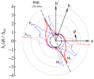
Figure 2: (Color online) Upper critical fields of s-wave FFLO state at $T=0$ scaled by zero-field gap $\Delta_{{\rm s}0}$. The red dot-dashed, blue solid, red thick solid, and blue dashed curves show the results for parameter sets ${\rm A}_{\rm ave}$, ${\rm P}_{\rm ave}$, ${\rm M}_{\rm 1}$, and ${\rm M}_{\rm 2}$, respectively. The dashed straight line represents the direction of the magnetic field ($-63.3^{\circ}$) at which the experimental $T_{\rm c}^{\rm onset}(\phi)$ has a maximum value for $H=30~{}{\rm kOe}$. [7] The bold dashed circle shows the Pauli paramagnetic limit $h_{\rm P}/\Delta_{\rm s0}=1/\sqrt{2}\approx 0.7071$.

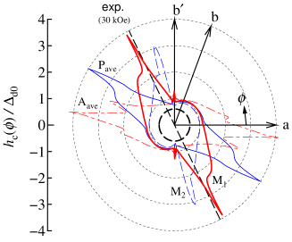
Figure 3: (Color online) Upper critical fields of d-wave FFLO state at $T=0$. The legend of this figure is similar to that of Fig. 2, except for the pairing symmetry and the values of the Pauli paramagnetic limit $h_{\rm P}/\Delta_{\rm d0}$, which are approximately equal to $0.6075$, $0.6096$, $0.6063$, and $0.6070$ for ${\rm P}_{\rm ave}$, ${\rm A}_{\rm ave}$, ${\rm M}_{\rm 1}$, and ${\rm M}_{\rm 2}$, respectively, whose curves coincide within the line width.

Results – Figures 2 and 3 show the $h_{\rm c}(\phi)$ of the s-wave and d-wave FFLO states, respectively. Over wide ranges of $\phi$, the upper critical fields $h_{\rm c}(\phi)$ are remarkably enhanced by the emergence of the FFLO state. In particular, they exhibit sharp cusps, at the tops of which $h_{\rm c}$ is more than six times the Pauli paramagnetic limit. [40] Their sharpness implies that the directions of the cusps must remain the optimum directions of the magnetic field that stabilize the FFLO state the most when the orbital pair-breaking effect is incorporated. The optimum directions are sensitive to changes in the inter-chain hopping integrals, whereas for all parameter sets, they are in the second and fourth quadrants, which do not contain the directions of $\pm{{\bm{b}}}$. This agrees with the observations in $T_{\rm c}^{\rm onset}(\phi)$. The parameter sets ${\rm M}_{\rm 1}$ and ${\rm M}_{\rm 2}$ give the maxima of $h_{\rm c}(\phi)$ near $\phi\approx 63.3^{\circ}$ and $78.3^{\circ}$, at which the experimental $T_{\rm c}^{\rm onset}(\phi)$ have the maximum values when $H=30$ and $47.5~{}{\rm kOe}$, respectively. Comparing Figs. 2 and 3, it is found that the optimum directions of $\phi$ do not strongly depend on the pairing symmetry.

At the cusps, it is easily verified that $n=3$, which means the terms in $\Delta k_{{\rm F}x}(k_{y},{{\bm{q}}})$ proportional to $(k_{y}-k_{y}^{0})^{1}$ and $(k_{y}-k_{y}^{0})^{2}$ vanish. This behavior is essentially the same as that in the square lattice system mentioned above, [19] although the controlling parameters ($\phi$ and $n_{\rm h}$) are different.

In Fig. 4, it is found that at each $\phi$, the Fermi surfaces touch or nearly touch when $q$ is optimized. At $\phi\approx-0.340\pi$, which is close to the optimum $\phi$, the red closed circle shows that the optimum $q$ makes the Fermi surfaces touch. For this point, Figs. 5(a) and (b) depict the Fermi surfaces and optimum ${{\bm{q}}}$ (the given $\phi$ and optimum $q$). Interestingly, at a $\phi$ value for which the two red thin dashed curves are very close, such as at $\phi\approx-0.210\pi$ (the blue closed triangle), the optimum $q$ deviates from those curves, which means the Fermi surfaces cross for the optimum $q$. However, as shown in Fig. 5(c), those crossing Fermi surfaces are very close over a wide range of $k_{y}$, and their crossing angle is extremely small. Therefore, for most practical purposes, we can regard the Fermi surfaces as touching when $q$ is optimized.

Figure 5 also shows that the points at which the Fermi surfaces touch are far away from $k_{y}=\pi/2$, near which the anion order affects the electron dispersion. Hence, the anion order would not significantly change the present result. [29].

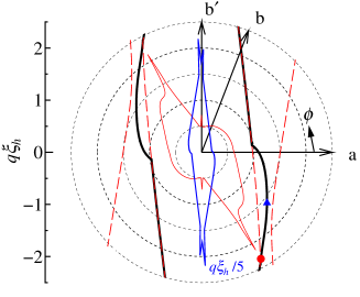
Figure 4: (Color online) Angular dependence of optimum $q(\phi)$ for parameter set ${\rm M}_{\rm 1}$ and d-wave pairing. $\xi_{h}(\phi)\equiv v_{\rm F}^{0}/2h_{\rm c}(\phi)$ and $v_{\rm F}^{0}\equiv t_{\rm S1}t_{\rm S2}a/\hbar[t_{\rm S1}^{2}+t_{\rm S2}^{2}]^{1/2}$ are defined. [41] The blue solid curve shows the value divided by five. The red dashed curves show the $q(\phi)$ values that make the Fermi surfaces touch. The red closed circle and blue closed triangle show the optimum $q(\phi)$ at $\phi=-0.340\pi$ and $-0.210\pi$, respectively. For these points, the Fermi surfaces are depicted in Figs. 5(a) and (b) and Fig. 5(c), respectively. The former is close to the $\phi$ at which $h_{\rm c}(\phi)$ is a maximum. For reference, the critical field is shown by the red thin solid curve in an arbitrary scale.

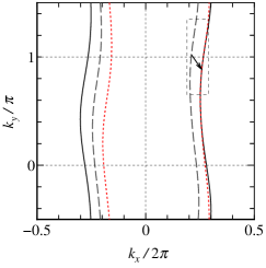
(a)	(b)	(c)

Figure 5: (Color online) Fermi-surface nesting when parameter set ${\rm M}_{\rm 1}$ is assumed. In panels (a) and (b) and panel (c), $\phi_{{{\bm{q}}}}=-0.340\pi$ and $-0.210\pi$ (i.e., $\varphi_{{{\bm{q}}}}=-0.3070\pi$ and $-0.1200\pi$), for which $h_{\rm c}\approx 3.895\Delta_{\rm d0}$ and $1.738\Delta_{\rm d0}$, respectively. The solid and dashed curves represent the Fermi surfaces of the holes with up and down spins, respectively. The red thin dotted and blue thin dashed curves represent the Fermi surfaces of the holes with down spins that are shifted by the vectors ${{\bm{q}}}$ (the small arrows), whose lengths maximize $h_{\rm c}$ for the given values of $\phi$. The $k_{x}$- and $k_{y}$-axes are drawn perpendicular to each other. In the present weak coupling theory, $h\ll t_{\rm S1}$; however, for this figure, we used a large value $h=0.1t_{\rm S1}$ to make the displacement visible.

Discussion – The discrepancy between the theoretical and experimental results is due to the simplifications in the present theory and lack of accurate information on the model parameters. For example, although the optimum direction of ${{\bm{H}}}$ depends on the magnitude of the magnetic field in the experimental observations, that is not so in the present theory. This discrepancy may be improved if the orbital pair-breaking effect and order-parameter mixing [23] are incorporated. A more precise analysis that incorporates these factors is left for future research.

Although we found parameter sets consistent with the observations, the ranges of the parameters that reproduce the experimental results have not been clarified. The relation between the optimum direction and hopping parameters will be examined in a separate paper.

Conclusion – In Q1D systems, the FFLO state is extremely stable for in-plane field directions around the nontrivial optimum directions indicated by the cusps in $h_{\rm c}(\phi)$. Interestingly, this behavior with cusps where $\phi$ is controlled is analogous to that in a square lattice system in which $n_{\rm h}$ is controlled to deform the Fermi surfaces. Hence, a similar behavior can occur in other low-dimensional systems with other controlling parameters. For ${\rm(TMTSF)_{2}ClO_{4}}$, it was shown that there exist realistic parameter sets (${\rm M}_{\rm 1}$ and ${\rm M}_{\rm 2}$) that can reproduce the optimum directions of ${{\bm{H}}}$ ($\parallel{{\bm{q}}}$) consistent with the experimental observations. Furthermore, for the parameter sets obtained from previous studies (${\rm P}_{\rm ave}$ and ${\rm A}_{\rm ave}$), the optimum directions are in the quadrants consistent with the experimental observations. These results are consistent with the hypothesis that the FFLO state emerges in the Q1D organic superconductor ${\rm(TMTSF)_{2}ClO_{4}}$.