ReNets: The Art of Reconfigurable Network Design

Self-Adjusting Networks

ReNets: Reconfigurable Routable Networks

DDANs: Dynamic Demand-Aware Networks

Routing Meets Entropy Bounds:
Dynamic Demand-Aware Networks

Theoretical Foundations for Self-Adjusting Networks (SANs)

Toward Demand-Aware Networking:
A Theory for Self-Adjusting Networks

Abstract.

The physical topology is emerging as the next frontier in an ongoing effort to render communication networks more flexible. While first empirical results indicate that these flexibilities can be exploited to reconfigure and optimize the network toward the workload it serves and, e.g., providing the same bandwidth at lower infrastructure cost, only little is known today about the fundamental algorithmic problems underlying the design of reconfigurable networks. This paper initiates the study of the theory of demand-aware, self-adjusting networks. Our main position is that self-adjusting networks should be seen through the lense of self-adjusting datastructures. Accordingly, we present a taxonomy classifying the different algorithmic models of demand-oblivious, fixed demand-aware, and reconfigurable demand-aware networks, introduce a formal model, and identify objectives and evaluation metrics. We also demonstrate, by examples, the inherent advantage of demand-aware networks over state-of-the-art demand-oblivious, fixed networks (such as expanders).

1. Introduction

Data-centric applications, including online services like web search, social networks, storage, financial services, multimedia, etc. (survey2017datacenter, ), as well as emerging applications such as distributed machine learning, generate a significant amount of network traffic (talk-about, ; kraken, ; dist-ml, ; singh2015jupiter, ; cisco-pro, ). It is hence not surprising that the design of efficient datacenter networks has received much attention over the last years. The topologies underlying modern datacenter networks range from trees (clos, ; fat-free, ) over hypercubes (bcube, ; mdcube, ) to expander networks (xpander, ) and provide high connectivity at low cost (survey2017datacenter, ).

Until now, these networks also have in common that their topology is fixed and oblivious to the actual demand (i.e., workload or communication pattern) they currently serve. As such, topologies are designed to provide worst-case guarantees, such as full bisection bandwidth, and to support arbitrary (all-to-all) communication patterns (clos, ).

Emerging technologies in like optical circuit switches (helios, ; rotornet, ; reactor, ; mordia, ), 60 GHz wireless communication (zhou2012mirror, ; kandula2009flyways, ) and free-space optics (firefly, ; projector, ) herald a very different kind of network topologies: malleable topologies which can be quickly reconfigured (singla2010proteus, ). Reconfigurable networks introduce an additional degree of freedom to the datacenter network design problem (singla2010proteus, ; projector, ; Jia2017, ; reactor, ; helios, ; firefly, ; zhou2012mirror, ; augmenting, ; chen2014osa, ).

The technology enables demand-aware networks which are optimized toward the workload they serve, statically (fixed topology) or even dynamically (reconfigurable topology) over time. We will refer to the latter also as self-adjusting networks. While first empirical studies show that a demand-aware network can achieve performance similar to a demand-oblivious network at lower cost (firefly, ; projector, ), not much is known today about the algorithmic problems underlying the design of self-adjusting networks. Indeed, while reconfigurable networks introduce an interesting paradigm shift, we currently lack analytical tools to investigate their potential and implications.

This paper initiates the study of the theory of demand-aware, self-adjusting networks, and in particular their fundamental underlying algorithmic problems. Our position is that self-adjusting networks should be seen from the perspective of self-adjusting datastructures: The current paradigm shift toward “self-optimizing” network topologies resembles the process that data structures went through over 40 years ago (splaytrees, ), evolving from static worst-case designs toward demand-aware and then self-adjusting designs, see Fig. 1.

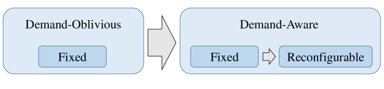
Figure 1. Simple taxonomy of network optimization

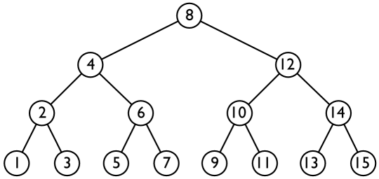
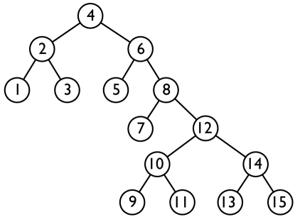
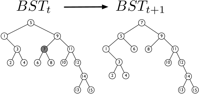
(a) BST: demand-oblivious	(b) BST: demand-aware	(c) BST: self-adjusting

Figure 2. Examples of different demand graphs and their corresponding networks

As an illustrative and well-studied example, consider the case of Binary Search Trees (BSTs), see Fig. 2. Traditional BSTs are (demand-)oblivious and do not rely on any assumptions on the demand (e.g., lookup requests) they serve, but optimize for the worst-case, where any item could be accessed: items are stored at distance $O(\log{n})$ from the root, uniformly and independently of their frequency, see Fig. 2 (a).

Clearly, if the demand has a specific pattern, the performance of the binary search tree designed for the worst case, is no longer optimal. Demand-aware (statically-)optimized but fixed BSTs (a.k.a. biased search trees) such as (Mehlhorn75, ; knuth1971optimum, ; hu1971optimal, ; bent1985biased, ) account for the frequency of the accessed items: frequent items are stored close to the root, infrequent items are lower in the tree, see Fig. 2 (b).

Self-adjusting BSTs, or dynamic demand-aware BSTs, are an attractive alternative to fixed BSTs, as they do not rely on an a priori knowledge about the demand. Rather, self-adjusting BSTs learn and adjust to the demand, and to its temporal locality, in an online manner. This, by now classical, approach was first introduced by Sleator and Tarjan (splaytrees, ) for splay trees, and today, several other self-adjusting BSTs exists, such as tango trees (tangotrees, ). As we will discuss later, despite not knowing the demand ahead of time, self-adjusting BSTs ideally never perform much worse than any fixed tree, but can perform significantly better if the demand features spatial or temporal locality.

In the same spirit, we in this paper present a taxonomy and a formal model for Self-Adjusting Networks (SANs). We show that while the performance of demand-oblivious networks is limited by worst-case metrics such as the network diameter, self-adjusting networks are only limited by the spatial and temporal locality. The more “structure” the demand has, the better self-adjusting networks can perform compared to demand-oblivious networks. We demonstrate by examples the inherent benefit of demand-aware networks over state-of-the-art demand-oblivious networks such as expander graphs, identify objectives, define desirable properties and metrics of demand-aware networks, and discuss open problems.

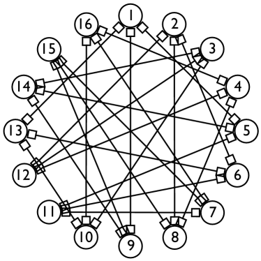
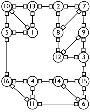
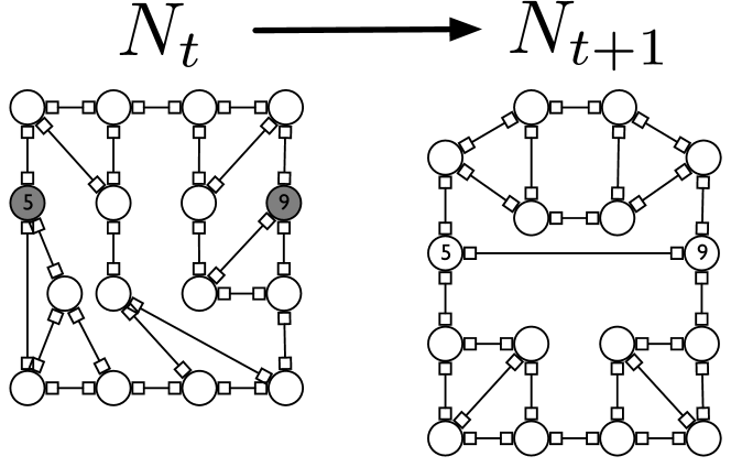
(a) Network: demand-oblivious	(b) Network: demand-aware	(c) Network: self-adjusting

Figure 3. Examples of different demand graphs and their corresponding networks.

2. Why Self-Adjusting Networks?

The vision of self-adjusting networks can be best understood by an analogy to datastructures. This section establishes and motivates this connection, and elaborates on the example of Binary Search Trees (BSTs) and a case study of routing. We will first demonstrate the benefits of self-adjusting BSTs and later extend the example to self-adjusting networks.

2.1. From Self-Adjusting Datastructures…

We can identify three different kinds of binary search tree datastructures: demand-oblivious BSTs, (static) demand-aware BSTs, and (dynamic) demand-aware BSTs, henceforth also called self-adjusting BSTs. We assume that the BST stores a set of items $\{1,2,\ldots,n\}$ where $n=2^{k}-1$.

Let us start by focusing on the most basic operation supported by a BST: the $\mathrm{search}()$ operation (for simplicity, we ignore $\mathrm{insert}()$ and $\mathrm{delete}()$). The cost of a search for an item $v$ is proportional to the depth of $v$ from the root of the BST (e.g., the number of pointer accesses). In graph terms, regarding the BST as a network, this corresponds to the shortest path length between the root and the searched element, $v$.

Now consider a demand to be served by the BST, given as a sequence of $m$ search requests $\tau=(\tau_{0},\tau_{1},\dots\tau_{m-1})$ for items (i.e., keys). $\tau$ is the problem input. For demonstration purposes, in the following, we will assume the specific search sequence $\tau=(1,1,\dots,1,3,3,\dots,3,5,5,\dots,5,\ldots,\ldots,2k-1,2k-1,\dots,2k-1)$ where an item is repeated many times consecutively. Note that $\tau$ contains $k=\log n$ unique items which correspond to the $k$ smallest leaves in the complete BST, see Fig. 2 (a).

Different BSTs, depending on whether they are demand-oblivious, static (fixed) demand-aware, and dynamic (reconfigurable) demand-aware, will incur different costs under this demand. In the following, we will examine the three different cases in turn.

Demand-Oblivious Datastructures. Let us first study a demand-oblivious BST, namely a tree that is designed to perform well even for a “worst possible” $\tau$. A balanced and complete BST over the items $1,\dots n$ provides an optimal solution for the demand-oblivious case, see Fig. 2 (a). Such a tree guarantees a cost of at most $\log n$ for every request in every sequence. Note that $\log n$ is also the maximum empirical entropy of an $n$-items sequence, where all items have the same (uniform) frequency. For our specific sequence $\tau$, which is unknown a priori, the amoritzed cost per request will be $\log n$: all items are leafs in the complete tree.

Demand-Aware Datastructures. Next, consider a (fixed) demand-aware BST which is optimized toward $\tau$ a priori, like in Fig. 2 (b). Such a demand-aware, optimized tree, can take advantage of the spatial locality of the demand, and will put all the $\log n$ requested items near the root (and other elements further away), resulting in an amoritzed cost of only about $\log\log n$ per request. Such optimized demand-aware trees have been studied, e.g., by Knuth (knuth1971optimum, ) and Hu et al. (hu1971optimal, ) who presented polynomial-time algorithms to construct exactly optimal trees for given probability distributions, as well as by Mehlhorn (Mehlhorn75, ) and Bent et al. (bent1985biased, ) who presented faster algorithms for approximately optimal trees. The amoritzed cost per request in these trees is proportional to the empirical entropy of the sequence, $\hat{H}(\tau)$. The empirical entropy is always $\hat{H}(\tau)\leq\log n$, and it can be much lower than $\log n$: in our example, $\hat{H}(\tau)\approx\log k=\log\log n$.

Self-Adjusting Datastructures. To conclude the example, let us consider a self-adjusting BST, as shown in Fig. 2 (c). For this case, the sequence is unknown a priory, but we can self-adjust the tree between requests. For every time $t$, we consider a (possibly) different binary search tree $BST_{t}$: we need a new operation, $\mathrm{adjust}()$, which reconfigures $BST_{t}$ to $BST_{t+1}$. Such an adjustment obviously comes at a cost, and is usually implemented using local tree rotations (each of constant cost) which preserve the search structure of the BST. More specifically, a tree rotation can only be performed for an accessed item and only by changing pointers with immediate neighbors (i.e., parents, children in the tree). Splay trees (splaytrees, ) for example, use a “move-to-front” rule, where the last requested item is rotated to the root, using tree rotations known as splay operations.

For the above considered sequence $\tau$, the amortized cost per request (including both $\mathrm{search}()$ and $\mathrm{adjust}()$) will be constant. Each requested item will move-to-front once, at high cost, but then this cost will be amoritzed by the subsequent repetitions of requests for the same item, taking advantage of temporal locality. Surprising at first, but by now well-known, is that for any sequence, splay trees are statically optimal: they perform as well as any demand-aware tree that is a priori optimized toward the demand, like Mehlhorn trees.

To summarize the BST example, for the above toy sequence $\tau$, the amortized cost per request will be about $\log n$ (for oblivious BSTs), $\log\log n$ (for demand-aware but static BSTs), or even constant (for self-adjusting BSTs), depending on the kind of BST. This clearly demonstrates the possible cost benefits of demand-aware and self-adjusting datastructures. For example, self-adjusting BSTs are useful for implementing caches and garbage collection where the principle of locality (denning2005locality, ) holds.

2.2. … to Self-Adjusting Networks

We now repeat the same motivation for networks. We look at a network as a datastructure that, rather than serving search requests issued from the root to an item, serves communication requests (e.g., packets) from a source node to a destination node. This operation is performed abstractly, via a $\mathrm{route}()$ operation, similar in spirit to the BST’s $\mathrm{search}()$ operation (where the source is always the root). The input to this routing problem is a sequence $\sigma=(\sigma_{0},\sigma_{1},\dots,\sigma_{m-1})$ of communication requests, where each request amounts to forwarding one unit of data from a source node $v$ to a destination node $u$. While network optimization in general obviously has many dimensions, and includes aspects such as addressing, policies, congestion, etc., in the following, we will only consider the routing or forwarding cost of each request: the cost of serving a request $\sigma_{i}$ is given by the length of the route from source to destination. In particular, in our example, we will assume shortest path routing.

Demand-Oblivious Networks. We start with the topologies of traditional demand-oblivious communication networks, which do not rely on any assumptions on the demand, $\sigma$. Rather, they are conservatively optimized for arbitrary (i.e., all-to-all) demands, providing worst-case properties such as bounded network diameter, mincut, or (almost) full bisection bandwidth (even in the presence of traffic engineering flexibilities (fat-free, )). Fig. 3 (a) presents an example for such a state-of-the-art network, an expander-based network (hoory, ; xpander, ).

What will be the amortized cost (i.e., the average route length) per request on such an expander? To start with a simple example (and for the sake of simplicity and clarity, we leave out some of the details), consider a demand $\sigma$ whose communication pattern is described by a two-dimensional square grid, of size $\sqrt{n}\times\sqrt{n}$ (see Fig. 4 (a)). We call this representation a demand graph $G(\sigma)$ where each weighted (directed) edge $e=(v,u)$ in the graph represents the frequency at which the two endpoints of $e$, namely $v$ and $u$, communicate in $\sigma$. Note that in this request sequence $\sigma$, every node communicates with at most four partners, hence, it is a sparse sequence, with spatial locality.

Serving this demand on a static expander in an oblivious (i.e., arbitrary) way will result in an average route length in the order of $\log n$, the diameter of a bounded degree expander. Note again that $\log n$ is the maximum empirical entropy of the demand, $H(\sigma)$.

Demand-Aware Networks. What about demand-aware networks? Can the average route length be better than $\log n$ if the network is optimized toward the demand $\sigma$ known a priori, as in Fig. 3 (b)? It turns out that the answer is affirmative for many cases, as was shown recently in (dan, ). A fundamental metric for the performance of such demand-aware networks turned out to be the (empirical) conditional entropy of $\sigma$. In a nutshell, the conditional entropy is a measure of the spatial locality of $\sigma$. In our example in Fig. 4 (a), since every node communicates with at most four partners (other nodes), the conditional entropy is a constant. In other words, there is a large gap of $\Theta(\log{n})$ between the conditional entropy and the entropy of $\sigma$. Clearly, a demand-aware network can be designed to serve our $\sigma$ at a very low (amortized) cost per request. The results in (dan, ) prove that if $G(\sigma)$ is sparse, then the conditional entropy is both a lower and an upper bound for the average route length; the paper presents a design that matches the upper bound. Another example introducing a large gap of $\Theta(\log{n})$ between demand-oblivious and demand-aware networks is a demand graph $G(\sigma)$ which forms a star (with unbounded degree), see Fig. 4 (b): node pairs communicate at different frequencies (skewed distribution, as indicated by the thickness). For this demand, the conditional entropy could be much lower than $\log n$ which will be the cost of serving this demand on an oblivious expander.

More generally, one can see that every sparse communication pattern which is embedded on a demand-oblivious expander, will result in average route lengths in the order of $\Omega(\log{n})$, the diameter, regardless of the entropy or the conditional entropy of the demand.

Self-Adjusting Networks. We complete the analogy by moving to self-adjusting networks, see Fig. 3 (c). Similar to the BST case, we have a new operation, $\mathrm{adjust}()$, to reconfigure the network at time $t$, $N_{t}$, to a new network at time $t+1$, $N_{t+1}$. This reconfiguration will also come at a cost that needs to be well-defined (and to be compared to the routing cost).

Like in BSTs, we can ask: is there a design of a self-adjusting network that achieves the bounds of an optimal fixed network, without knowledge of $\sigma$, but using reconfigurations in an online manner? In other words, are there statically optimal self-adjusting networks? Like splay trees are for binary search trees?

Moreover, similarly to BSTs, we note that self-adjusting networks, taking advantage both of spatial and temporal locality, can in principle perform much better than existing cost lower bounds (such as (dan, )) for static demand-aware networks. For example one can think of requests that arrive from a grid like in Fig. 4 (a), but where the grid also changes over time, to add temporal locality. For this case, self-adjusting networks will perform better than static networks.

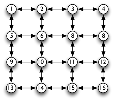
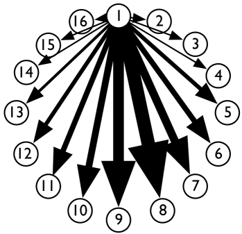
(a)	(b)

Figure 4. Expander networks do not achieve optimal average route lengths for sparse demand graphs. (a) An oblivious embedding of a 2-dimensional grid demand graph on a constant degree expander network will result in average route lengths of $\Omega(\log n)$, while the conditional entropy of the demand graph is less than two. (b) An oblivious embedding of a weighted star demand graph on a constant degree expander network will result in an average route length of $\Omega(\log n)$, while the conditional entropy of the demand graph could be much lower.

3. Taxonomy

This section presents a more systematic taxonomy of network designs, revolving around the (demand) awareness, the type of topology (fixed or reconfigurable), the type of input (e.g., unknown, known, revealed online over time), as well as the required algorithms and properties. See Fig. 5.

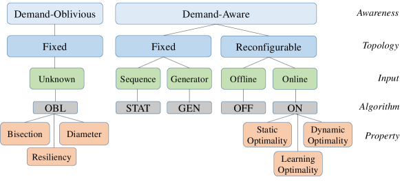
Figure 5. Detailed taxonomy of network optimization

3.1. Demand-Oblivious Networks

State-of-the-art demand-oblivious datacenter networks such as Xpander (xpander, ) rely on a fixed (static) network topology and are not optimized toward a specific demand: the demand (i.e., input) is unknown. Typical objectives of such network designs are to provide (almost) full bisection bandwidth (assuming all-to-all communication patterns), short routes (e.g., at most 6 hops from server to top-of-the-rack switch, aggregation switch, core, and down again), as well as resiliency (e.g., $k$-connectivity). We will refer to algorithms for demand-oblivious networks by Obl.

3.2. Demand-Aware Networks

Fixed Demand-Aware Networks. The input to the fixed (static) demand-aware network design problem could either be a sequence of requests (in our case, communication requests) $\sigma$ or a generative model $\mathcal{G}$ (generator) of such requests. A generator $\mathcal{G}$ comes with a set of parameters $\mathrm{par}(\mathcal{G})$. A most simple example for a generative model is a fixed distribution from which requests are sampled i.i.d.: such a generator may feature spatial locality, however, it does not feature any temporal locality as requests are sampled independently. A more complex generative model which also features temporal locality could be, for example, a Markovian process (or random walk).

Independently of whether the input is a sequence or generator, our goal is to design an optimal fixed topology $N^{*}$, and we will refer to the corresponding algorithms as Stat and Gen.

Reconfigurable Demand-Aware Networks. Reconfigurable demand-aware networks allow to optimize the topology at runtime, i.e., the topology is dynamic. If the demand is known a priori, an offline algorithm Off can be used to compute an optimized schedule to reconfigure a network over time, i.e., unlike Stat, Off changes the network over time and is charged for such reconfigurations. In other words, Off should only change the network when it pays off later, by making requests cheaper to serve.

Most interesting are scenarios where the input is not known a priori but revealed over time, in an online manner. We distinguish between three important metrics: static optimality, learning optimality, and dynamic optimality. We have already discussed static optimality above: it asks for an online algorithm On which is competitive compared to an optimal static algorithm Stat. In contrast, dynamic optimality asks for an algorithm On which is competitive even when compared to an optimal (dynamic) offline algorithm Off, a much stronger requirement.

An interesting special case regards a scenario in which the demand is fixed but not known ahead of time, and the goal of the online network reconfiguration algorithm is to learn the demand generator quickly and cost-effieciently (with little reconfigurations). For example, if the demand is given by a generator describing a fixed distribution from which requests are sampled i.i.d., ideally, an algorithm would quickly converge to an optimized fixed network which optimally serves this distribution: since requests are i.i.d., there is no temporal locality and reconfigurations are no longer beneficial after convergence. If the generator is a Markov process, the request sequence may feature both spatial and temporal locality, and an algorithm should quickly learn the process and may then converge to an optimal reconfiguration schedule over time. We hence introduce a third type of optimality besides static and dynamic optimality: learning optimality. Learning optimality asks for an online algorithm On which is competitive compared to an optimal static algorithm Gen which knows the generator.

Finally, we can classify algorithms for online reconfigurable demand-aware networks in two flavors: centralized algorithms and distributed (i.e., decentralized and concurrent) algorithms.

3.3. Additional Properties

Besides the properties that are specific to demand-aware networks, it is usually desirable that demand-aware networks additionally still fulfill the traditional properties of demand-oblivious networks, for example the requirement to provide redundant connectivity. Furthermore, some static properties become more useful in the dynamic conext, for example, compact and local routing: As dynamic demand-aware networks may change frequently over time, it may be highly undesirable to recompute routing paths each time for each topological modification; rather, it would be ideal if the topology allows to forward packets greedily, at any time, and modifications only entail local changes to the forwarding tables.

4. A Formal Model

This section presents a general algorithmic model for self-adjusting networks. We consider a set of $n$ nodes $V=\{1,\ldots,n\}$ (e.g., the top-of-rack switches). The communication demand among these nodes is a sequence $\sigma=(\sigma_{1},\sigma_{2},\ldots)$ of communication requests where $\sigma_{t}=(u,v)\in V\times V$, is a source-destination pair. The communication demand can either be finite or infinite.

In order to serve this demand, the nodes $V$ must be inter-connected by a network $N$, defined over the same set of nodes. In case of a demand-aware network, $N$ can be optimized towards $\sigma$, either statically or dynamically: a self-adjusting network $N$ can change over time, and we denote by $N_{t}$ the network at time $t$, i.e., the network evolves: $N_{0},N_{1},N_{2},\ldots$

4.1. Constraints

In addition to the dynamic properties related to optimizations over time, described shortly, a network $N_{t}$ may have to adhere to some physical constraints (e.g., the number of lasers which can be installed on a top-of-the-rack switch may be limited) and fulfill invariants at any time. This can be modeled by requiring that all networks $N_{t}$ belong to some network family $\mathcal{N}$: $N_{t}\in\mathcal{N}$. Examples for families $\mathcal{N}$ may include, bounded degree networks (e.g., for a high scalability), networks of full bisection bandwidth or expanders (e.g., to ensure congestion-free shuffle phases), $k$-connected networks (for resiliency), etc.

4.2. Reconfiguration

The crux of designing smart self-adjusting networks is to find an optimal tradeoff between the benefits and the costs of reconfiguration: while by reconfiguring the network, we may be able to serve requests more efficiently in the future, reconfiguration itself can come at a cost.

The inputs to the self-adjusting network design problem is a set of allowed network topologies $\mathcal{N}$, the request sequence $\sigma=(\sigma_{0},\sigma_{1},\ldots,\sigma_{m-1})$, and two types of costs:

• An adjustment cost $\mathrm{adj}:\mathcal{N}\times\mathcal{N}\rightarrow\mathbb{R}$ which defines the cost of reconfiguring a network $N$ to a network $N^{\prime}$. Adjustment costs may include mechanical costs (e.g., energy required to move lasers or abrasion) as well as performance costs (e.g., reconfiguring a network may entail control plane overheads or packet reorderings, which can harm throughput). For example, the cost could be given by the number of links which need to be changed in order to transform the network.

• A service cost $\mathrm{srv}:\sigma\times\mathcal{N}\rightarrow\mathbb{R}$ which defines, for each request $\sigma_{i}$ and for each network $N\in\mathcal{N}$, what is the price of serving $\sigma_{i}$ in network $N$. For example, the cost could correspond to the route length: shorter routes require less resources and hence reduce not only load (e.g., bandwidth consumed along fewer links), but also energy consumption, delay, and flow completion times, could be considered for example.

Serving request $\sigma_{i}$ under the current network configuration $N_{i}$ will hence cost $\mathrm{srv}(\sigma_{i},N_{i})$, after which the network reconfiguration algorithm may decide to reconfigure the network at cost $\mathrm{adj}(N_{i},N_{i+1})$. The total processing cost of a schedule $\sigma$ is then

$$\mathrm{Cost}(\mathcal{A},N_{0},\sigma)=\sum_{i=0}^{m-1}\mathrm{srv}(\sigma_{i},N_{i})+\mathrm{adj}(N_{i},N_{i+1})$$

where $N_{i}\in\mathcal{N}$ denotes the network at time $i$.

It is sometimes useful to aggregate the requests of sequence $\sigma$ over time and represent it as a directed and weighted demand graph (resp. guest graph or request graph) $G(\sigma)=(V(\sigma),E(\sigma))$.

We need the concept of amortized costs to reason about costs over sequences.

Definition 0 (Average and Amortized Cost).

Given an algorithm $\mathcal{A}$, an initial network $N_{0}$, a reconfiguration cost function $\mathrm{adj}$, a request serving cost function $\mathrm{srv}$, and a sequence $\sigma=(\sigma_{0},\sigma_{1},\ldots,\sigma_{m-1})$ of communication requests over time, we define the (average) cost incurred by $\mathcal{A}$ as:

$$\mathrm{Cost}(\mathcal{A},N_{0},\sigma)=\frac{1}{m}\sum_{i=0}^{m-1}\mathrm{srv}(\sigma_{i},N_{i})+\mathrm{adj}(N_{i},N_{i+1})$$

where $N_{i}\in\mathcal{N}$ denotes the network at time $i$. The amortized cost of $\mathcal{A}$ is defined as the worst possible cost of $\mathcal{A}$ over all initial networks $N_{0}$ and all sequences $\sigma$, i.e., $\max_{N_{0},\sigma}\mathrm{Cost}(\mathcal{A},N_{0},\sigma)$.

4.3. Objectives and Metrics

We can now define static, dynamic, and learning optimality objectives. In static optimality, want the network to (asymptotically) perform well even in hindsight, i.e., given knowledge of the demand.

Definition 0 (Static Optimality).

Let Stat be an optimal static algorithm with perfect knowledge of the demand $\sigma$, and let On be an online algorithm. We say that On is statically optimal if, for sufficiently long communication patterns $\sigma$, the following ratio is constant:

$$\rho=\max_{\sigma}\frac{\mathrm{Cost}(\textsc{On},N_{0},\sigma)}{\mathrm{Cost}(\textsc{Stat},N^{*},\sigma)}+\beta$$

for some $\beta$ independent of the length of the sequence $\sigma$. Here, $N_{0}\in\mathcal{N}$ is the initial network, from which  On starts, and $N^{*}\in\mathcal{N}$ is the statically optimal network. In other words, On’s cost is at most a constant factor higher than Stat’s in the worst case.

The holy grail of self-adjusting networks however regards the design of dynamically optimal reconfigurable networks: how well can a reconfigurable demand-aware network perform, when compared to a network which is dynamically optimized in an offline manner?

Definition 0 (Dynamic Optimality).

An algorithm is called dynamically optimal if and only if it is asymptotically optimal even compared to an optimal offline algorithm which can dynamically reconfigure the network and which has complete knowledge of the request sequence $\sigma$ ahead of time. More formally, let Off be an optimal offline algorithm, and let On be an online algorithm. We say that On is dynamically optimal if the following ratio is constant:

$$\rho=\max_{\sigma}\frac{\mathrm{Cost}(\textsc{On},N_{0},\sigma)}{\mathrm{Cost}(\textsc{Off},N_{0},\sigma)}$$

that is, On’s cost is at most $\rho$ times higher in the worst case. Again, $N_{0}\in\mathcal{N}$ is the initial network.

Finally, we define learning optimality which lies between the above:

Definition 0 (Learning Optimality).

An algorithm (which initially does not know the parameters $\mathrm{par}(\mathcal{G})$ of the generator) is called learning optimal if and only if it is asymptotically optimal even when compared to an optimal static algorithm which knows the generator. More formally, let Stat be an optimal fixed algorithm, and let Gen be an online learning algorithm. We say that Gen is learning optimal if the following ratio of expectations is constant:

$$\rho=\max_{\mathrm{par}(\mathcal{G})}\frac{\mathbb{E}[\mathrm{Cost}(\textsc{On},N_{0},\sigma)]}{\mathbb{E}[\mathrm{Cost}(\textsc{Gen},N^{*},\sigma)]}+\beta$$

where $\beta$ is independent of the length of the sequence and where the maximum is taken over the parameters of the generator model $\mathcal{G}$. That is, Gen’s cost is at most $\rho$ times higher in the worst case.

5. Review of State-of-the-Art

The problem of designing demand-aware and self-adjusting networks is a fundamental one, and finds interesting applications in many distributed and networked systems, not only in datacenters. For example, use cases also arise in the context of wide-area networks (Jia2017, ; jin2016optimizing, ) and, more traditionally, in the context of overlays (scheideler2009distributed, ; ratnasamy2002topologically, ). However, while the problem is natural, surprisingly little is known today about the design of demand-aware networks, especially dynamic networks which can change over time. The approach of reconfiguring network topologies to reduce communication costs, is orthogonal to approaches changing the traffic matrix itself (e.g., (fibium, )) or migrating communication endpoints on a fixed topology (disc16, ).

One basic observation to make is that the design of static demand-aware networks is related to graph embedding problems (a.k.a. virtual network embedding and graph layout problems) (diaz2002survey, ; ifip18round, ; bansal2011minimum, ): given a graph (describing the demand), find an embedding in another graph (the physical topology), such that certain properties are fulfilled (e.g., the sum or max of the total load on the physical graph is minimized). It is known that the embedding problem is NP-hard in many variants (ifip18landscape, ), for example already for very simple physical networks such as the line (diaz2002survey, ): the problem of embedding an arbitrary request graph onto a line is known as the Minimum Linear Arrangement (MLA) problem. From this relationship it also follows that the static offline demand-aware network design problem is NP-hard if the designed network is restricted to the family of degree-2 networks.

However, unlike graph embedding problems, in the design of demand-aware networks, the physical network is not given but subject to optimization as well. An intriguing and open question is whether this additional degree of freedom makes the problem harder or easier. An encouraging example (focusing on routing) is given in (splaynets, ): an optimal fixed demand-aware network (also called DAN in the literature) restricted to BSTs can be computed in polynomial time. Another example of approximately optimal demand-aware networks are Dans (dan, ) (which provide a constant approximation for sparse demand graphs), matching the lower bounds based on conditional entropies derived in the same paper. A slightly different model, motivated by optical switches which can be configured to provide an optimized matching, is studied in (ancs18, ): the authors present several optimal algorithms for special workloads (e.g., where the demand is given by a single flow). There is also work on resilient demand-aware networks, such as rDan (rdan, ) (based on a coding approach but without degree bounds).

Even less is known about self-adjusting networks. The best upper bound known so far for online reconfigurable networks is $O(\hat{H}(X_{\sigma})+\hat{H}(Y_{\sigma}))$, where $\hat{H}(X_{\sigma})$ and $\hat{H}(Y_{\sigma})$ are the empirical entropies of sources and destinations in $\sigma$, respectively (ton15splay, ). It is achieved by a self-adjusting tree network (the tree network can also be decentralized (displaynets, )). While this is optimal for some frequency distributions (e.g., the empirical distribution of $\sigma$), and in particular product frequency distributions, in general, it can be far from optimal.

6. Conclusion

We hope that our paper can nourish the ongoing discussions on the benefits and limitations of such reconfigurable network topologies, and we believe that our work opens many interesting questions for future research. On the algorithmic front, a first important open question concerns the design of a self-adjusting network that achieves the bounds of a static network, without knowledge of $\sigma$, but using reconfigurations in an online manner: are there statically optimal self-adjusting networks, like splay trees are for binary search trees? Similarly, the design of learning optimal and dynamically optimal demand-aware networks remains an open problem. The latter is particularly challenging: in the context of datastructures, the problem of designing dynamically optimal BSTs has been an open problem for many decades already (tangotrees, ).

On the modeling front, further refinements are required to account for the specific costs incurred by a self-adjusting network. In particular, today, we lack good models for the cost of reconfiguration of networks: costs may not only accrue in terms of, e.g., energy needed for the reconfiguration but also in terms of performance: as routing over a continuously changing topology can be challenging, it is desirable that (multi-hop) routing can be performed locally, i.e., greedily, without the need for (distributed) forwarding table recomputations. This property is called local routing. Furthermore, models need to be extended to account for other quantitative aspects such as load.

Acknowledgments. We thank Monia Ghobadi and Robert Tarjan for inputs and discussions.

References

- (1) M. Noormohammadpour and C. S. Raghavendra, “Datacenter traffic control: Understanding techniques and trade-offs,” IEEE Communications Surveys & Tutorials, 2017.
- (2) J. C. Mogul and L. Popa, “What we talk about when we talk about cloud network performance,” SIGCOMM Comput. Commun. Rev. (CCR), vol. 42, pp. 44–48, Sept. 2012.
- (3) C. Fuerst, S. Schmid, L. Suresh, and P. Costa, “Kraken: Online and elastic resource reservations for multi-tenant datacenters,” in Proc. IEEE INFOCOM, 2016.
- (4) Mu Li et al., “Scaling distributed machine learning with the parameter server.,” in Proc. USENIX OSDI, vol. 14, pp. 583–598, 2014.
- (5) A. Singh, J. Ong, A. Agarwal, G. Anderson, A. Armistead, R. Bannon, S. Boving, G. Desai, B. Felderman, P. Germano, et al., “Jupiter rising: A decade of clos topologies and centralized control in google’s datacenter network,” Proc. ACM SIGCOMM Computer Communication Review (CCR), vol. 45, no. 4, pp. 183–197, 2015.
- (6) Cisco, “Cisco global cloud index: Forecast and methodology, 2015-2020,” White Paper, 2015.
- (7) M. Al-Fares, A. Loukissas, and A. Vahdat, “A scalable, commodity data center network architecture,” in Proc. ACM SIGCOMM Computer Communication Review (CCR), vol. 38, pp. 63–74, 2008.
- (8) A. Singla, “Fat-free topologies,” in Proc. ACM Workshop on Hot Topics in Networks (HotNets), pp. 64–70, 2016.
- (9) C. Guo, G. Lu, D. Li, H. Wu, X. Zhang, Y. Shi, C. Tian, Y. Zhang, and S. Lu, “Bcube: a high performance, server-centric network architecture for modular data centers,” Proc. ACM SIGCOMM Computer Communication Review (CCR), vol. 39, no. 4, pp. 63–74, 2009.
- (10) H. Wu, G. Lu, D. Li, C. Guo, and Y. Zhang, “Mdcube: a high performance network structure for modular data center interconnection,” in Proc. ACM International Conference on Emerging Networking Experiments and Technologies (CONEXT), pp. 25–36, 2009.
- (11) S. Kassing, A. Valadarsky, G. Shahaf, M. Schapira, and A. Singla, “Beyond fat-trees without antennae, mirrors, and disco-balls,” in Proc. ACM SIGCOMM, pp. 281–294, 2017.
- (12) N. Farrington, G. Porter, S. Radhakrishnan, H. H. Bazzaz, V. Subramanya, Y. Fainman, G. Papen, and A. Vahdat, “Helios: a hybrid electrical/optical switch architecture for modular data centers,” Proc. ACM SIGCOMM Computer Communication Review (CCR), vol. 40, no. 4, pp. 339–350, 2010.
- (13) W. M. Mellette, R. McGuinness, A. Roy, A. Forencich, G. Papen, A. C. Snoeren, and G. Porter, “Rotornet: A scalable, low-complexity, optical datacenter network,” in Proc. ACM SIGCOMM, pp. 267–280, 2017.
- (14) H. Liu, F. Lu, A. Forencich, R. Kapoor, M. Tewari, G. M. Voelker, G. Papen, A. C. Snoeren, and G. Porter, “Circuit switching under the radar with reactor.,” in Proc. USENIX Symposium on Networked Systems Design and Implementation (NSDI), vol. 14, pp. 1–15, 2014.
- (15) G. P. R. S. N. Farrington, A. F. P. Chen-Sun, T. R. Y. F. G. Papen, and A. Vahdat, “Integrating microsecond circuit switching into the data center,” 2013.
- (16) X. Zhou, Z. Zhang, Y. Zhu, Y. Li, S. Kumar, A. Vahdat, B. Y. Zhao, and H. Zheng, “Mirror mirror on the ceiling: Flexible wireless links for data centers,” Proc. ACM SIGCOMM Computer Communication Review (CCR), vol. 42, no. 4, pp. 443–454, 2012.
- (17) S. Kandula, J. Padhye, and P. Bahl, “Flyways to de-congest data center networks,” in Proc. ACM Workshop on Hot Topics in Networks (HotNets), 2009.
- (18) N. Hamedazimi, Z. Qazi, H. Gupta, V. Sekar, S. R. Das, J. P. Longtin, H. Shah, and A. Tanwer, “Firefly: A reconfigurable wireless data center fabric using free-space optics,” in Proc. ACM SIGCOMM Computer Communication Review (CCR), vol. 44, pp. 319–330, 2014.
- (19) M. Ghobadi et al., “Projector: Agile reconfigurable data center interconnect,” in Proc. ACM SIGCOMM, pp. 216–229, 2016.
- (20) A. Singla, A. Singh, K. Ramachandran, L. Xu, and Y. Zhang, “Proteus: a topology malleable data center network,” in Proc. ACM Workshop on Hot Topics in Networks (HotNets), 2010.
- (21) S. Jia, X. Jin, G. Ghasemiesfeh, J. Ding, and J. Gao, “Competitive analysis for online scheduling in software-defined optical wan,” in Proc. IEEE INFOCOM, 2017.
- (22) D. Halperin, S. Kandula, J. Padhye, P. Bahl, and D. Wetherall, “Augmenting data center networks with multi-gigabit wireless links,” in Proc. ACM SIGCOMM, 2011.
- (23) K. Chen, A. Singla, A. Singh, K. Ramachandran, L. Xu, Y. Zhang, X. Wen, and Y. Chen, “Osa: An optical switching architecture for data center networks with unprecedented flexibility,” IEEE/ACM Transactions on Networking (TON), vol. 22, no. 2, pp. 498–511, 2014.
- (24) D. D. Sleator and R. E. Tarjan, “Amortized efficiency of list update and paging rules,” Commun. ACM, vol. 28, pp. 202–208, Feb. 1985.
- (25) K. Mehlhorn, “Nearly optimal binary search trees,” Acta Inf., vol. 5, pp. 287–295, 1975.
- (26) D. E. Knuth, “Optimum binary search trees,” Acta informatica, vol. 1, no. 1, pp. 14–25, 1971.
- (27) T. C. Hu and A. C. Tucker, “Optimal computer search trees and variable-length alphabetical codes,” SIAM Journal on Applied Mathematics, vol. 21, no. 4, pp. 514–532, 1971.
- (28) S. W. Bent, D. D. Sleator, and R. E. Tarjan, “Biased search trees,” SIAM Journal on Computing, vol. 14, no. 3, pp. 545–568, 1985.
- (29) E. D. Demaine, D. Harmon, J. Iacono, and M. Patrascu, “Dynamic optimality - almost,” SIAM J. Comput., vol. 37, no. 1, pp. 240–251, 2007.
- (30) P. J. Denning, “The locality principle,” Communications of the ACM, vol. 48, no. 7, pp. 19–24, 2005.
- (31) S. Hoory, N. Linial, and A. Wigderson, “Expander graphs and their applications,” ulletin of the American Mathematical Society, vol. 43, 2006.
- (32) C. Avin, K. Mondal, and S. Schmid, “Demand-aware network designs of bounded degree,” in Proc. International Symposium on Distributed Computing (DISC), 2017.
- (33) X. Jin, Y. Li, D. Wei, S. Li, J. Gao, L. Xu, G. Li, W. Xu, and J. Rexford, “Optimizing bulk transfers with software-defined optical wan,” in Proc. ACM SIGCOMM, pp. 87–100, 2016.
- (34) C. Scheideler and S. Schmid, “A distributed and oblivious heap,” Proc. International Conference on Automata, Languages and Programming (ICALP), pp. 571–582, 2009.
- (35) S. Ratnasamy, M. Handley, R. Karp, and S. Shenker, “Topologically-aware overlay construction and server selection,” in Proc. IEEE INFOCOM, vol. 3, pp. 1190–1199, 2002.
- (36) N. Sarrar, S. Uhlig, A. Feldmann, R. Sherwood, and X. Huang, “Leveraging zipf’s law for traffic offloading,” Proc. ACM SIGCOMM Computer Communication Review (CCR), vol. 42, no. 1, pp. 16–22, 2012.
- (37) C. Avin, A. Loukas, M. Pacut, and S. Schmid, “Online balanced repartitioning,” in Proc. 30th International Symposium on Distributed Computing (DISC), 2016.
- (38) J. Díaz, J. Petit, and M. Serna, “A survey of graph layout problems,” ACM Computing Surveys (CSUR), vol. 34, no. 3, pp. 313–356, 2002.
- (39) M. Rost and S. Schmid, “Virtual network embedding approximations: Leveraging randomized rounding,” in Proc. IFIP Networking, 2018.
- (40) N. Bansal, K.-W. Lee, V. Nagarajan, and M. Zafer, “Minimum congestion mapping in a cloud,” in Proc. 30th Annual ACM Symposium on Principles of Distributed Computing (PODC), pp. 267–276, 2011.
- (41) M. Rost and S. Schmid, “Charting the complexity landscape of virtual network embeddings,” in Proc. IFIP Networking, 2018.
- (42) S. Schmid, C. Avin, C. Scheideler, M. Borokhovich, B. Haeupler, and Z. Lotker, “Splaynet: Towards locally self-adjusting networks,” IEEE/ACM Transactions on Networking (ToN), 2016.
- (43) K.-T. Foerster, M. Ghobadi, and S. Schmid, “Characterizing the algorithmic complexity of reconfigurable data center architectures,” in Proc. ACM/IEEE Symposium on Architectures for Networking and Communications Systems (ANCS), 2018.
- (44) C. Avin, A. Hercules, A. Loukas, and S. Schmid, “rdan: Toward robust demand-aware network designs,” in Information Processing Letters (IPL), 2018.
- (45) S. Schmid, C. Avin, C. Scheideler, M. Borokhovich, B. Haeupler, and Z. Lotker, “Splaynet: Towards locally self-adjusting networks,” IEEE/ACM Transactions on Networking (ToN), to appear.
- (46) B. Peres, O. Goussevskaia, S. Schmid, and C. Avin, “Concurrent self-adjusting distributed tree networks,” in Proc. International Symposium on Distributed Computing (DISC), 2017.