Automatic Classification of Defective Photovoltaic Module Cells in Electroluminescence Images

Abstract

Electroluminescence (EL) imaging is a useful modality for the inspection of photovoltaic (PV) modules. EL images provide high spatial resolution, which makes it possible to detect even finest defects on the surface of PV modules. However, the analysis of EL images is typically a manual process that is expensive, time-consuming, and requires expert knowledge of many different types of defects.

In this work, we investigate two approaches for automatic detection of such defects in a single image of a PV cell. The approaches differ in their hardware requirements, which are dictated by their respective application scenarios. The more hardware-efficient approach is based on hand-crafted features that are classified in a Support Vector Machine (SVM). To obtain a strong performance, we investigate and compare various processing variants. The more hardware-demanding approach uses an end-to-end deep Convolutional Neural Network (CNN) that runs on a Graphics Processing Unit (GPU). Both approaches are trained on $1{,}968$ cells extracted from high resolution EL intensity images of mono- and polycrystalline PV modules. The CNN is more accurate, and reaches an average accuracy of $88.422{,}818{,}791{,}9\text{\,}\mathrm{\char 37\relax}\text{/}$. The SVM achieves a slightly lower average accuracy of $82.438{,}478{,}75\text{\,}\mathrm{\char 37\relax}\text{/}$, but can run on arbitrary hardware. Both automated approaches make continuous, highly accurate monitoring of PV cells feasible.

marginparwidth=1.5cm,marginparsep=8mm *[enumerate]label=(0) pt

1 Introduction

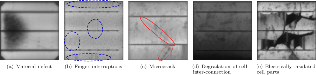
Figure 1: Various intrinsic and extrinsic defects in monocrystalline (LABEL:fig:material-defect–LABEL:fig:gridfinger-defect) and polycrystalline (LABEL:fig:crack-defect–LABEL:fig:deep-crack-defect) solar cells. LABEL:fig:material-defect shows a solar cell with a typical material defect. LABEL:fig:gridfinger-defect shows finger interruptions in the encircled areas, which do not necessarily reduce the module efficiency. The solar cell in LABEL:fig:crack-defect contains a microcrack that is very subtle in its appearance. While microcracks do not divide the cell completely, they still must be detected because such cracks may grow over time and eventually impair the module efficiency. The spots at the bottom of this cell are likely to indicate cell damage as well. However, such spots can be oftentimes difficult to distinguish from actual material defects. LABEL:fig:disconnected-cell-defect shows a disconnected area due to degradation of the cell interconnection. LABEL:fig:deep-crack-defect shows a cell with electrically separated or degraded parts, which are usually caused by mechanical damage.

Solar modules are usually protected by an aluminum frame and glass lamination from environmental influences such as rain, wind, and snow. However, these protective measures can not always prevent mechanical damages caused by dropping the PV module during installation, impact from falling tree branches, hail, or thermal stress. Also, manufacturing errors such as faulty soldering or defective wires can also result in damaged PV modules. Defects can in turn decrease the power efficiency of solar modules. Therefore, it is necessary to monitor the condition of solar modules, and replace or repair defective units in order to ensure maximum efficiency of solar power plants.

Visual identification of defective units is particularly difficult, even for trained experts. Aside from obvious cracks in the glass, many defects that reduce the efficiency of a PV module are not visible to the eye. Conversely, defects that are visible do not necessarily reduce the module efficiency.

To precisely determine the module efficiency, the electrical output of a module must be measured directly. However, such measurements require manual interaction with individual units for diagnosis, and hence they do not scale well to large solar power plants with thousands of PV modules. Additionally, such measurements only capture one point in time, and as such may not reveal certain types of small cracks, which will become an issue over time [1].

Infrared (IR) imaging is a non-destructive, contactless alternative to direct measurements for assessing the quality of solar modules. Damaged solar modules can be easily identified by solar cells which are either partially or completely cut off from the electric circuit. As a result, the solar energy is not converted into electricity anymore, which heats the solar cells up. The emitted infrared radiation can then be imaged by an IR camera. However, IR cameras are limited by their relatively low resolution, which can prohibit detection of small defects such as microcracks not yet affecting the photoelectric conversion efficiency of a solar module.

Electroluminescence (EL) imaging [2, 3] is another established non-destructive technology for failure analysis of PV modules with the ability to image solar modules at a much higher resolution. In EL images, defective cells appear darker, because disconnected parts do not irradiate. To obtain an EL image, current is applied to a PV module, which induces EL emission at a wavelength of $1{,}150\text{\,}\mathrm{nm}\text{/}$. The emission can be imaged by a silicon Charge-coupled Device (CCD) sensor. The high spatial image resolution enables the detection of microcracks [4], and EL imaging also does not suffer from blurring due to lateral heat propagation. However, visual inspection of EL images is not only time-consuming and expensive, but also requires trained specialists. In this work, we remove this constraint by proposing an automated method for classifying defects in EL images.

In general, defects in solar modules can be classified into two categories [3]: 1. intrinsic deficiencies due to material properties such as crystal grain boundaries and dislocations, and 2. process-induced extrinsic defects such as microcracks and breaks, which reduce the overall module efficiency over time.

Figure 1 shows an example EL image with different types of defects in monocrystalline and polycrystalline solar cells. LABEL:fig:material-defect and LABEL:fig:gridfinger-defect show general material defects from the production process such as finger interruptions which do not necessarily reduce the lifespan of the affected solar panel unless caused by high strain at the solder joints [5]. Specifically, the efficiency degradation induced by finger interruptions is a complex interaction between their size, position, and the number of interruptions [6, 5]. LABEL:fig:crack-defect to LABEL:fig:deep-crack-defect show microcracks, degradation of cell-interconnections, and cells with electrically separated or degraded parts that are well known to reduce the module efficiency. Particularly the detection of microcracks requires cameras with high spatial resolution.

Figure 2: Defect probabilities inferred for each PV module cell by the proposed CNN. A darker shade of red indicates a higher likelihood of a cell defect.

For the detection of defects during monitoring one can set different goals. Highlighting the exact location of defects within a solar module allows to monitor affected areas with high precision. However, the exact defect location within the solar cell is less important for the quality assessment of a whole PV module. For this task, the overall likelihood indicating a cell defect is more important. This enables a quick identification of defective areas and can potentially complement the prediction of future efficiency loss within a PV module. In this work, we propose two classification pipelines that automatically solve the second task, i.e., to determine a per-cell defect likelihood that may lead to efficiency loss.

The investigated classification approaches in this work are SVM and CNN classifiers.

Support Vector Machines (SVMs)

are trained on various features extracted from EL images of solar cells.

Convolutional Neural Network (CNN)

is directly fed with image pixels of solar cells and the corresponding labels.

The SVM approach is computationally particularly efficient during training and inference. This allows to operate the method on a wide range of commodity hardware, such as tablet computers or drones, whose usage is dictated by the respective application scenario. Conversely, the prediction accuracy of the CNN is generally higher, while training and inference is much more time-intensive and commonly requires a GPU for an acceptably short runtime. Particularly for aerial imagery, however, additional issues may arise and will need to be solved. Kang and Cha [7] highlight several challenges that need to be addressed before applying our approach outside of a manufacturing setting.

1.1 Contributions

The contribution of this work consists of three parts. First, we present a resource-efficient framework for supervised classification of defective solar cells using hand-crafted features and an SVM classifier that can be used on a wide range of commodity hardware, including tablet computers and drones equipped with low-power single-board computers. The low computational requirements make the on-site evaluation of the EL imagery possible, similar to analysis of low resolution IR images [8]. Second, we present a supervised classification framework using a convolutional neural network that is slightly more accurate, but requires a GPU for efficient training and classification. In particular, we show how uncertainty can be incorporated into both frameworks to improve the classification accuracy. Third, we contribute an annotated dataset consisting of $2{,}624$ aligned solar cells extracted from high resolution EL images to the community, and we use this dataset to perform an extensive evaluation and comparison of the proposed approaches.

Figure 2 exemplarily shows the assessment results of a solar panel using the proposed convolutional neural network. Each solar cell in the EL image is overlaid by the likelihood of a defect in the corresponding cell.

1.2 Outline

The remainder of this work is organized as follows. Related work is reviewed in Section 2. Section 3 introduces both proposed classification approaches. In Section 4, we evaluate and compare these approaches, and discuss the results. This work is concluded in Section 5.

2 Related Work

Figure 3: An overview of the SVM classification pipeline with the four proposed variations of the preprocessing and feature extraction process.

Visual inspection of solar modules via EL imaging is an active research topic. Most of the related work, however, focuses on the detection of specific intrinsic or extrinsic defects, but not on the prediction of defects that eventually lower the power efficiency of solar modules. Detection of surface abnormalities in EL images of solar cells is related to structural health monitoring. However, it is important to note that certain defects in solar cells are only specific to EL imaging of PV modules. For instance, fully disconnected solar cells simply appear as dark image regions (similar to LABEL:fig:disconnected-cell-defect) and thus have no comparable equivalent in terms of structural defects. Additionally, surface irregularities in solar wafers (such as finger interruptions) are easily confused with cell cracks, even though they do not significantly affect the power loss.

In the context of visual inspection of solar modules, Tsai et al. [9] use Fourier image reconstruction to detect defective solar cells in EL images of polycrystalline PV modules. The targeted extrinsic defects are (small) cracks, breaks, and finger interruptions. Fourier image reconstruction is applied to remove possible defects by setting high-frequency coefficients associated with line- and bar-shaped artifacts to zero. The spectral representation is then transformed back into the spatial domain. The defects can then be identified as intensity differences between the original and the high-pass filtered image. Due to the shape assumption, the method has difficulties detecting defects with more complex shapes.

Tsai et al. [10] also introduced a supervised learning method for identification of defects using Independent Component Analysis (ICA) basis images. Defect-free solar cell subimages are used to find a set of independent basis images with ICA. The method achieves a high accuracy of $93.4\text{\,}\mathrm{\char 37\relax}\text{/}$ with a relatively small training dataset of $300$ solar cell subimages. However, material defects such as finger interruptions are treated equally to cell cracks. This strategy is therefore only suitable for detection of every abnormality on the surface of solar cells, but not for the prediction of future energy loss.

Anwar and Abdullah [11] developed an algorithm for the detection of microcracks in polycrystalline solar cells. They use anisotropic diffusion filtering followed by shape analysis to localize the defects in solar cells. While the method performs well at detecting microcracks, it does not consider other defect types such as completely disconnected cells, which appear completely dark in EL images.

Tseng et al. [12] proposed a method for automatic detection of finger interruptions in monocrystalline solar cells. The method employs binary clustering of features from candidate regions for the detection of defects. Finger interruptions, however, do not necessarily provide suitable cues for prediction of future power loss.

The success of deep learning led to a gradual replacement of traditional pattern recognition pipelines for optical inspection. However, to our knowledge, no CNN architecture has been proposed for EL images, but only for other modalities or applications. Most closely related is the work by Mehta et al. [13], who presented a system for predicting the power loss, localization and type of soiling from RGB images of solar modules. Their approach does not require manual localization labels, but instead operates on images with the corresponding power loss as input. Masci et al. [14] proposed an end-to-end max-pooling CNN for classifying steel defects. Their network performance is compared against multiple hand-crafted feature descriptors that are trained using SVMs. Although their dataset consists of only $2{,}281$ training and $646$ test images, the CNN architecture classifies steel defects at least twice as accurately as the SVMs. Zhang et al. [15] proposed a CNN architecture for detection of cracks on roads. To train the CNN, approximately $45{,}000$ hand-labeled image patches were used. They show that CNNs greatly outperform hand-crafted features classified by a combination of an SVM and boosting. Cha et al. [16] use a very similar approach to detect concrete cracks in a broad range of images taken under various environmental and illumination conditions. Kang and Cha [7] employ deep learning for structural health monitoring on aerial imagery. Cha et al. [17] additionally investigated defect localization using the modern learning-based segmentation approaches for region proposals based on the Faster R-CNN framework which can perform in real-time. Lee et al. [18] also use semantic segmentation to detect cracks in concrete.

In medical context, Esteva et al. [19] employ deep neural networks to classify different types of skin cancer. They trained the CNN end-to-end on a large dataset consisting of $129{,}450$ clinical images and $2{,}032$ different diseases making it possible to achieve a high degree of accuracy.

3 Methodology

We subdivide each module into its solar cells, and analyze each cell individually to eventually infer the defect likelihood. This breaks down the analysis to the smallest meaningful unit, in the sense that the mechanical design of PV modules interconnects units of cells in series. Also, the breakdown considerably increases the number of available data samples for training. For the segmentation of solar cells, we use a recently developed method [20], which brings every cell into a normal form free of perspective and lens distortions.

Unless otherwise stated, the proposed methods operate on size-normalized EL images of solar cells with a resolution of $300\times 300$ pixels. This image resolution was derived from the median dimensions of image regions corresponding to individual solar cells in the original EL images of PV modules. The solar cell images are used directly as pipeline input. The image resolution of solar cells in the wild will generally deviate from the required resolution and therefore must be adjusted accordingly. The CNN architecture sets a minimum image resolution, which typically equals the CNN’s receptive field (, the original Vgg-19 architecture uses $224\times 224$). If the resolution is lower than this minimum resolution, then the image must be upscaled. For higher resolutions, the network can be applied in a strided window manner and afterwards the outputs are pooled together (typically using average or maximum pooling). We followed an alternative approach in which the CNN architecture encodes this process inherently. In case of the SVM pipeline, the resolution requirement is less stringent. Given local features that are scale-invariant, the image resolution of the classified solar cells does not need to be adjusted and may vary from image to image.

3.1 Classification Using Support Vector Machines

The general approach for classification using SVMs [21] is as follows. First, local descriptors are extracted from images of segmented PV cells. The features are typically extracted at salient points, also known as keypoints, or from a dense pixel grid. For training the classifier and subsequent predictions, a global representation needs to be computed from the set of local descriptors, oftentimes referred to as encoding. Finally, this global descriptor for a solar cell is classified into defective or functional. Figure 3 visualizes the classification pipeline, consisting of masking, keypoint detection, feature description, encoding, and classification. We describe these steps in the following subsections.

3.1.1 Masking

We assume that the solar cells were segmented from a PV module, , using the automated algorithm we proposed in earlier work [20]. A binary mask allows then to separate the foreground of every cell from the background. The cell background includes image regions that generally do not belong to the silicon wafer, such as the busbars and the inter-cell borders. This mask can be used to strictly limit feature extraction to the cell interior. In the evaluation, we investigate the usefulness of masking, and find that its effect is minor, , it only slightly improves the performance in a few feature/classifier combinations.

3.1.2 Feature Extraction

Figure 4: Two different feature extraction strategies applied to the same PV cell with and without masking. In LABEL:fig:pv-cell-dense-sampling, keypoints are sampled at fixed positions specified by the center of a cell in the overlaid grid. LABEL:fig:pv-cell-masked-dense-points uses equally sized and oriented keypoints laid out on a dense grid similar to LABEL:fig:pv-cell-dense-sampling. LABEL:fig:pv-cell-keypoint-detection shows an example for AGAST keypoints (detection threshold slightly increased for visualization). LABEL:fig:pv-cell-masked-keypoint-detection shows KAZE keypoints of various sizes and orientations after masking out the background area.

In order to train the SVMs, feature descriptors are extracted first. The locations of these local features are determined using two main sampling strategies: (1) keypoint detection, and (2) dense sampling. These strategies are exemplarily illustrated in Fig. 4. Both strategies produce different sets of features that can be better suitable for specific types of solar wafers than others. Dense sampling disregards the image content and instead uses a fixed configuration of feature points. Keypoint detectors, on the other hand, rely on the textureness in the image and therefore the number of keypoints is proportional to the amount of high-frequency elements, such as edges and corners (as can be seen in LABEL:fig:pv-cell-keypoint-detection and LABEL:fig:pv-cell-masked-keypoint-detection). Keypoint detectors typically operate in scale space, allowing feature detection at different scale levels and also at different orientations. LABEL:fig:pv-cell-masked-keypoint-detection shows keypoints detected by KAZE. Here, each keypoint has a different scale (visualized by the radius of corresponding circles) and also a specific orientation exemplified by the line drawn from the center to the circle border. Keypoints that capture both the scale and the rotation are invariant to changes in image resolution and to in-plane rotations, which makes them very robust.

Dense sampling subdivides the $300\times 300$ pixels PV cell by overlaying it with a grid consisting of $n\times n$ cells. The center of each grid cell specifies the position at which a feature descriptor will be subsequently extracted. The number of feature locations only depends on the grid size. Dense sampling can be useful if computational resources are very limited, or if the purpose is to identify defects only in monocrystalline PV modules.

We employ different popular combinations of keypoint detectors and feature extractors from the literature, as listed in Table 1 and outlined below.

Table 1: Investigated keypoint detectors and feature descriptors. SIFT, SURF, and KAZE (in bold) contain both a detector and a descriptor. We explored also combinations of the keypoint detectors of AGAST and KAZE with other feature descriptors. Note, the keypoints provided by SIFT and SURF were not reliable enough and thus not further evaluated.

Method	Keypoint detector	Feature descriptor
AGAST [22]	✓	✗
KAZE [23]	✓	✓
HOG [24]	✗	✓
PHOW [25]	✗	✓
SIFT [26]	(✓)	✓
SURF [27]	(✓)	✓
VGG [28]	✗	✓

Several algorithms combine keypoint detection and feature description. Probably the most popular of these methods is Scale-invariant Feature Transform (SIFT) [26], which detects and describes features at multiple scales. SIFT is invariant to rotation, translation, and scaling, and partially resilient to varying illumination conditions. Speeded Up Robust Features (SURF) [27] is a faster variant of SIFT, and also consists of a keypoint detector and a local feature descriptor. However, the detector part of SURF is not invariant to affine transformations. In initial experiments, we were not able to successfully use the keypoint detectors of SIFT and SURF, because the keypoint detector at times failed to detect features in relatively homogeneous monocrystalline cell images, and hence we used only the descriptor parts.

KAZE [23] is a multiscale feature detector and descriptor. The keypoint detection algorithm is very similar to SIFT, except that the linear Gaussian scale space used by SIFT is replaced by nonlinear diffusion filtering. For feature description, however, KAZE uses the SURF descriptor.

We also investigated Adaptive and Generic Accelerated Segment Test (AGAST) [22] as a dedicated keypoint detector without descriptor. It is based on a random forest classifier trained on a set of corner features that is known as Features from Accelerated Segment Test (FAST) [29, 30].

Among the dedicated descriptors, Pyramid Histogram of Visual Words (PHOW) [25] is an extension of SIFT that computes SIFT descriptors densely over a uniformly spaced grid. We use the implementation variant from Vlfeat [31]. Similarly, Histogram of Oriented Gradients (HOG) [24] is a gradient-based feature descriptor computed densely over a uniform set of image blocks. Finally, we also used the Visual Geometry Group (VGG) descriptor trained end-to-end using an efficient optimization method [28]. In our implementation, we employ the 120-dimensional real-valued descriptor variant.

We omitted binary descriptors from this selection. Even though binary feature descriptors are typically very fast to compute, they generally do not perform better than real-valued descriptors [32].

3.1.3 Combinations of Detectors and Extractors

For the purpose of determining the most powerful feature detector/extractor combination, we evaluated all feature detector and feature extractor combinations with few exceptions.

In most cases, we neither tuned the parameters of keypoint detectors nor those of feature extractors but rather used the defaults by Opencv [33] as of version 3.3.1. One notable exception is Adaptive and Generic Accelerated Segment Test (AGAST), where we lowered the detection threshold to 5 to be able to detect keypoints in monocrystalline PV modules. For SIFT and SURF, similar adjustments were not successful, which is why we only used their descriptors. HOG requires a grid of overlapping image regions, which is incompatible with the keypoint detectors. Instead, we downsampled the $300\times 300$ pixels cell images to $256\times 256$ pixels (the closest power of 2) for feature extraction. Masking was omitted for HOG due to implementation-specific limitations. Given these exceptions, we overall evaluate twelve feature combinations.

3.1.4 Encoding

The computed features are encoded into a global feature descriptor. The purpose of encoding is the formation of a single, fixed-length global descriptor from multiple local descriptors. Encoding is commonly represented as a histogram that draws its statistics from a background model. To this end, we employ Vectors of Locally Aggregated Descriptors (VLAD) [34], which offers a compact state-of-the-art representation [35]. VLAD encoding is sometimes also used for deep learning based features in classification, identification and retrieval tasks [36, 37, 38, 39].

The VLAD dictionary is created by $k$-means clustering of a random subset of feature descriptors from the training set. For performance reasons, we use the fast mini-batch variant [40] of $k$-means. The cluster centroids $\bm{\mu}_{k}$ correspond to anchor points of the dictionary. Afterwards, first order statistics are aggregated as a sum of residuals of all descriptors $\mathcal{X}\coloneqq\{\bm{x}_{t}\in\mathbb{R}^{d}\mid t=1,\dotsc,T\}$ extracted from a solar cell image. The residuals are computed with respect to their nearest anchor point $\bm{\mu}_{k}$ in the dictionary $D\coloneqq\{\bm{\mu}_{k}\in\mathbb{R}^{d}\mid k=1,\dotsc,K\}$ as

$$\bm{\nu}_{k}\coloneqq\sum_{t=1}^{T}\eta_{k}(\bm{x}_{t})(\bm{x}_{t}-\bm{\mu}_{k})$$ (1)

where $$\eta_{k}\colon\mathbb{R}^{d}\to\{0,1\}$$ is an indicator function to cluster membership, ,

$$\eta_{k}(\bm{x})\coloneqq\begin{dcases}1&\text{if}\leavevmode\nobreak\ k=\operatorname*{argmin}_{j=1,\dotsc,K}\lVert\bm{x}-\bm{\mu}_{j}\rVert_{2}\\ 0&\text{otherwise}\end{dcases}\enspace,$$ (2)

which indicates whether $\bm{x}$ is the nearest neighbor of $\bm{\mu}_{k}$. The final VLAD representation $\bm{\nu}\in\mathbb{R}^{Kd}$ corresponds to the concatenation of all residual terms (1) into a $Kd$-dimensional vector:

$$\bm{\nu}\coloneqq(\bm{\nu}^{\top}_{1},\ldots,\bm{\nu}^{\top}_{K})^{\top}\enspace.$$ (3)

Several normalization steps are required to make the VLAD descriptor robust. Power normalization addresses issues when some local descriptors occur more frequently than others. Here, each element of the global descriptor $v_{i}\in\bm{\nu}$ is normalized as

$$\hat{v}_{i}\coloneqq\operatorname*{sign}(v_{i})\lvert v_{i}\rvert^{\rho},\quad i=1,\dotsc,Kd$$ (4)

where we chose $\rho=0.5$ as a typical value from the literature. After power normalization, the vector is normalized such that its $\ell^{2}$-norm equals one.

Figure 5: Architecture of the modified Vgg-19 network used for prediction of defect probability in $300\times 300$ pixels EL images of solar cells. Boldface denotes layers that deviate from Vgg-19.

Similarly, an over-counting of co-occurrences can occur if at least two descriptors appear together frequently. Jégou and Ondřej [41] showed that Principal Component Analysis (PCA) whitening effectively eliminates such co-occurrences and additionally decorrelates the data.

To enhance the robustness of the codebook $D$ against potentially suboptimal solutions from the probabilistic $k$-means clustering, we compute five VLAD representations from different training subsets using different random seeds. Afterwards, the concatenation of the VLAD encodings $\tilde{\bm{\nu}}\coloneqq(\hat{\bm{\nu}}^{\top}_{1},\ldots,\hat{\bm{\nu}}^{\top}_{m})^{\top}\in\mathbb{R}^{mKd}$ is jointly decorrelated and whitened by means of PCA [42]. The transformed representation is again normalized such that its $\ell^{2}$-norm equals one and the result is eventually passed to the SVM classifier.

3.1.5 Support Vector Machine Training

We trained SVMs both with a linear and a Radial Basis Function (RBF) kernel. For the linear kernel, we use Liblinear [43], which is optimized for linear classification tasks and large datasets. For the non-linear RBF kernel, we use Libsvm [44].

The SVM hyperparameters are determined by evaluating the average $F_{1}$ score [45] in an inner five-fold cross-validation on the training set using a grid search. For the linear SVM, we employ the $\ell^{2}$ penalty on a squared hinge loss. The penalty parameter $C$ is selected from a set of powers of ten, , $C_{\text{linear}}\in\{10^{k}\mid k=-2,\dotsc,6\}\subset\mathbb{R}_{>0}$. For RBF SVMs, the penalty parameter $C$ is determined from a slightly smaller set $C_{\text{RBF}}\in\{10^{k}\mid k=2,\dotsc,6\}$. The search space of the kernel coefficient $\gamma$ is constrained to $\gamma\in\{10^{-7},10^{-6},S^{-1}\}\subset[0,1]$, where $S$ denotes the number of training samples.

3.2 Regression Using a Deep Convolutional Neural Network

We considered several strategies to train the CNN. Given the limited amount of data we had at our disposal, best results were achieved by means of transfer learning. We utilized the Vgg-19 network architecture [46] originally trained on the ImageNet dataset [47] using $1.28$ million images and $1{,}000$ classes. We then refined the network using our dataset.

We replaced the two fully connected layers of Vgg-19 by a Global Average Pooling (GAP) [48] and two fully connected layers with $4{,}096$ and $2{,}048$ neurons, respectively (, Fig. 5). The GAP layer is used to make the Vgg-19 network input tensor ($224\times 224\times 3$) compatible to the resolution of our solar cell image samples ($300\times 300\times 3$), in order to avoid additional downsampling of the samples. The output layer consists of a single neuron that outputs the defect probability of a cell. The CNN is refined by minimizing the Mean Squared Error (MSE) loss function. Hereby, we essentially train a deep regression network, which allows us to predict (continuous) defect probabilities trained using only two defect likelihood categories (functional and defective). By rounding the predicted continuous probability to the nearest neighbor of the four original classes, we can directly compare CNN decisions against the original ground truth labels without binarizing them.

Data augmentation is used to generate additional, slightly perturbed training samples. The augmentation variability, however, is kept moderate, since the segmented cells vary only by few pixels along the translational axes, and few degrees along the axis of rotation. The training samples are scaled by at most $2\text{\,}\mathrm{\char 37\relax}\text{/}$ of the original resolution. The rotation range is capped to $\pm$3\text{\,}\mathrm{\SIUnitSymbolDegree}\text{/}$$. The translation is limited to $\pm$2\text{\,}\mathrm{\char 37\relax}\text{/}$$ of the cell dimensions. We also use random flips along the vertical and horizontal axes. Since the busbars can be laid out both vertically and horizontally, we additionally include training samples rotated by exactly $90\text{\,}\mathrm{\SIUnitSymbolDegree}\text{/}$. The rotated samples are augmented the same way as described above.

We fine-tune the pretrained ImageNet model on our data to adapt the CNN to the new task, similar to Girshick et al. [49]. We, however, do this in two stages. First, we train only the fully connected layers with randomly initialized weights while keeping the weights of the convolutional blocks fixed. Here, we employ the Adam optimizer [50] with a learning rate of $10^{-3}$, exponential decay rates $\beta_{1}=0.9$ and $\beta_{2}=0.999$, and the regularization value $\hat{\epsilon}=10^{-8}$. In the second step, we refine the weights of all layers. At this stage, we use the Stochastic Gradient Descent (SGD) optimizer with a learning rate of $5\cdot 10^{-4}$ and a momentum of 0.9. We observed that fine-tuning the CNN in several stages by subsequently increasing the number of hyperparameters slightly improves the generalization ability of the resulting model compared to a single refinement step.

In both stages, we process the augmented versions of the $1{,}968$ training samples in mini-batches of 16 samples on two NVIDIA GeForce GTX 1080, and run the training procedure for a maximum of $100$ epochs. This totals to $196{,}800$ augmented variations of the original $1{,}968$ training samples that are used to refine the network. For the implementation of the deep regression network, we use Keras version 2.0 [51] with TensorFlow version 1.4 [52] in the backend.

4 Evaluation

For the quantitative evaluation, we first evaluate different feature descriptors extracted densely over a grid. Then, we compare the best configurations against feature descriptors extracted at automatically detected keypoints to determine the best performing variation of the SVM classification pipeline. Finally, we compare the latter against the proposed deep CNN, and visualize the internal feature mapping of the CNN.

4.1 Dataset

We propose a public dataset of solar cells extracted from high resolution EL images of monocrystalline and polycrystalline PV modules [53]. The dataset consists of $2{,}624$ solar cell images at a resolution of $300\times 300$ pixels originally extracted from $44$ different PV modules, where $18$ modules are of monocrystalline type, and $26$ are of polycrystalline type.

The images of PV modules used to extract the individual solar cell samples were taken in a manufacturing setting. Such controlled conditions enable a certain degree of control on quality of imaged panels and allow to minimize negative effects on image quality, such as overexposure. Controlled conditions are also required particularly because background irradiation can predominate EL irradiation. Given PV modules emit the only light during acquisition performed in a dark room, it can be ensured the images are uniformly illuminated. This is opposed to image acquisition in general structural health monitoring, which introduces additional degrees of freedom where images can suffer from shadows or spot lighting [16]. An important issue in EL imaging, however, can be considered blurry (, out-of-focus) EL images due to incorrectly focused lens which can be at times challenging to attain. Therefore, we ensured to include such images in the proposed dataset (, Fig. 1 for an example).

The solar cells exhibit intrinsic and extrinsic defects commonly occurring in mono- and polycrystalline solar modules. In particular, the dataset includes microcracks and cells with electrically separated and degraded parts, short-circuited cells, open inter-connects, and soldering failures. These cell defects are widely known to negatively influence efficiency, reliability, and durability of solar modules. Finger interruptions are excluded since the power loss caused by such defects is typically negligible.

Table 2: Partitioning of the solar cells into functional and defective, with an additional self-assessment on the rater’s confidence after visual inspection. Non-confident decisions obtain a weight lower than $100\text{\,}\mathrm{\char 37\relax}\text{/}$ for the evaluation of the classifier performance.

Condition	Confident?	Label $p$	Weight $w$
functional	✓	functional	$100\text{\,}\mathrm{\char 37\relax}\text{/}$
	✗	defective	$33\text{\,}\mathrm{\char 37\relax}\text{/}$
defective	✓	defective	$100\text{\,}\mathrm{\char 37\relax}\text{/}$
	✗	defective	$67\text{\,}\mathrm{\char 37\relax}\text{/}$

Measurements of power degradation were not available to provide the ground truth. Instead, the extracted cells were presented in random order to a recognized expert, who is familiar with intricate details of different defects in EL images. The criteria for such failures are summarized by Köntges et al. [5]. In their failure categorization, the expert focused specifically on defects with known power loss above $3\text{\,}\mathrm{\char 37\relax}\text{/}$ from the initial power output. The expert answered the questions (1) is the cell functional or defective? (2) are you confident in your assessment? The assessments into functional and defective cells by a confident rater were directly used as labels. Non-confident assessments of functional and defective cells were all labeled as defective. To reflect the rater’s uncertainty, lower weights are assigned to these assessments, namely a weight of $33\text{\,}\mathrm{\char 37\relax}\text{/}$ to a non-confident assessment of functional cell, and a weight of $67\text{\,}\mathrm{\char 37\relax}\text{/}$ to a non-confident assessment of defective cell. Table 2 shows this in summary, with the rater assessment on the left, and the associated classification labels and weights on the right. Table 3 shows the distribution of ground truth solar cell labels, separated by the type of the source PV module.

Table 3: The distribution of the total number of solar cell images in the dataset depending on sample label $p$ and the PV module type from which the solar cells were originally extracted. The numbers of solar cell images are given for the $75\text{\,}\mathrm{\char 37\relax}\text{/}$/$25\text{\,}\mathrm{\char 37\relax}\text{/}$ training/test split.

Solar wafer	Train				Test				$\Sigma$
	$0\text{\,}\mathrm{\char 37\relax}\text{/}$	$33\text{\,}\mathrm{\char 37\relax}\text{/}$	$67\text{\,}\mathrm{\char 37\relax}\text{/}$	$100\text{\,}\mathrm{\char 37\relax}\text{/}$	$0\text{\,}\mathrm{\char 37\relax}\text{/}$	$33\text{\,}\mathrm{\char 37\relax}\text{/}$	$67\text{\,}\mathrm{\char 37\relax}\text{/}$	$100\text{\,}\mathrm{\char 37\relax}\text{/}$
Monocrystalline	$438$	$87$	$41$	$249$	$150$	$30$	$15$	$64$	$1{,}074$
Polycrystalline	$683$	$132$	$37$	$301$	$237$	$46$	$13$	$101$	$1{,}550$
$\Sigma$	$1{,}121$	$219$	$78$	$550$	$387$	$76$	$28$	$165$	$2{,}624$

We used $25\text{\,}\mathrm{\char 37\relax}\text{/}$ of the labeled cells ($656$ cells) for testing, and the remaining $75\text{\,}\mathrm{\char 37\relax}\text{/}$ ($1{,}968$ cells) for training. Stratified sampling was used to randomly split the samples while retaining the distribution of samples within different classes in the training and the test sets. To further balance the training set, we weight the classes using the inverse proportion heuristic derived from King and Zeng [54]

$$c_{j}\coloneqq\frac{S}{2n_{j}}\enspace,$$ (5)

where $S$ is the total number of training samples, and $n_{j}$ is the number of functional ($j=0$) or defective ($j=1$) samples.

4.2 Dense Sampling

Figure 6: Classification performance for different dense sampling configurations in terms of $F_{1}$ score grouped by the feature descriptor, classifier, weighting strategy, and the use of masking. The highest $F_{1}$ score is achieved using a linear SVM and the VGG feature descriptor at a grid resolution of $65\times 65$ cells with sample weighting and masking (LABEL:pgfplots:dense-vgg-weighted-masked) LABEL:fig:dense-conf-vgg.

In this experiment, we evaluate different grid sizes for subdividing a single $300\times 300$ pixels cell image. The number of grid points per cell is varied between $5\times 5$ to $75\times 75$ points. At each grid point, SIFT, SURF, and VGG descriptors are computed. The remaining two descriptors, PHOW and HOG, are omitted in this experiment, because they do not allow to arbitrarily specify the position for descriptor computation. Note that at a $75\times 75$ point grid, the distance between two grid points is only 4 pixels, which leads to a significant overlap between neighbored descriptors. Therefore, further increase of the grid resolution cannot be expected to considerably improve the classification results.

The goal of this experiment is to find the best performing combination of grid size and classifier. We trained both linear SVMs and SVMs with the RBF kernel. For each classifier, we also examine two additional options, namely whether the addition of the sample weights $w$ ( Table 2) or masking out the background region ( Section 3.1.1) improves the classifiers.

Figure 7: Receiver Operating Characteristic (ROC) for top performing feature detector/extractor combinations grouped by mono-, polycrystalline, and both solar module types combined. The dashed curve () represents the baseline in terms of a random classifier. Note the logarithmic scale of the false positive rate axis. Refer to the text for details.

Performance is measured using the $F_{1}$ score, which is the harmonic mean of precision and recall. Figure 6 shows the $F_{1}$ scores that are averaged over the individual per-class $F_{1}$ scores. From left to right, these scores are shown for the SURF descriptor (LABEL:fig:dense-conf-surf), SIFT descriptor (LABEL:fig:dense-conf-sift) and VGG descriptor (LABEL:fig:dense-conf-vgg). Here, the VGG descriptor achieves the highest score on a grid of size $65\times 65$ using a linear SVM with weighting and masking. SIFT is the second best performing descriptor with best performance on a $60\times 60$ grid using linear SVM with weighting, but without masking. SURF achieved the lowest scores, with a peak at a $70\times 70$ grid using an RBF SVM with weighting, but without masking. The results show the trend that more grid points lead to better results. The classification accuracy of SURF increases only slowly and saturates at about $70\text{\,}\mathrm{\char 37\relax}\text{/}$. SIFT and VGG benefit more from denser grids. The use of the weights $w$ leads in most cases to a higher score, because the classifier can stronger rely on samples for which the expert labeler was more confident. Masking also improves the $F_{1}$ score for VGG features. However, the improvement by almost two percent is small compared to the overall performance variation over the configurations. One can argue that the cell structure is not substantial for distinguishing different kinds of cell defects given the high density of the feature points and the degree of overlap between image regions evaluated by feature extractors.

4.3 Dense Sampling vs. Keypoint Detection

This experiment aims at comparing the classification performance of dense grid-based features versus keypoint-based features. To this end, the best performing grid-based classifier per descriptor from the previous experiment are compared to combinations of keypoint detectors and feature descriptors.

Figure 8: ROC curves of the best performing KAZE/VGG feature detector/descriptor combination (LABEL:pgfplots:roc-baseline-mono) compared to the ROC of the deep regression network (LABEL:pgfplots:roc-cnn-mono). While in the monocrystalline case LABEL:fig:roc-final-mono the classification performance of the CNN is almost on par with the linear SVM. For polycrystalline PV modules LABEL:fig:roc-final-poly the CNN considerably outperforms SVM with the linear kernel trained on KAZE/VGG features. The latter outcome leads to a higher CNN ROC AUC for both PV modules types combined LABEL:fig:roc-final-overall. The dashed curve () represents the baseline in terms of a random classifier.

Figure 7 shows the evaluated detector and extractor combinations for monocrystalline cells, polycrystalline cells, and both together. Most detector/extractor combinations are specified by a forward slash (Detector/Descriptor). Entries without a forward slash, namely KAZE, HOG, and PHOW, denote features which already include both a detector and a descriptor. The three best performing methods on a dense grid are denoted as Dense SIFT $60\times 60$, Dense SURF $70\times 70$, and Dense VGG $65\times 65$, respectively. Unless otherwise specified, the features were trained with sample weighting, without masking, and using a linear SVM.

The performance is shown using ROC curves that indicate the performance of binary classifiers at various false positive rates [55]. Additionally, the plots show the AUC scores for the top-4 features with the highest AUC emphasized in bold. In all three cases, KAZE/VGG outperforms other feature combinations with an AUC of $88.51\text{\,}\mathrm{\char 37\relax}\text{/}$ on all modules, followed by KAZE/SIFT with an AUC of $87.217{,}544{,}683{,}884{,}9\text{\,}\mathrm{\char 37\relax}\text{/}$. As an exception, the second best feature combination for polycrystalline solar cells in terms of AUC is PHOW. The gray dashed curve represents the baseline in terms of a random classifier. Overall, the use of keypoints leads to better performance than dense sampling.

4.4 Support Vector Machine vs. Transfer Learning Using Deep Regression Network

Figure 8 shows the performance of the strongest SVM variant, KAZE/VGG, in comparison to the CNN classifier. The ROC curve on the left in LABEL:fig:roc-final-mono contains the results for monocrystalline PV modules. LABEL:fig:roc-final-poly in the center provides the classification performance for polycrystalline PV modules. Finally, the overall classification performance of both models is shown in LABEL:fig:roc-final-overall on the right.

Notably, the classification performance of SVM and CNN is very similar for monocrystalline PV modules. The CNN performs on average only slightly better than the SVM. At lower false positive rates around and below $1\text{\,}\mathrm{\char 37\relax}\text{/}$, the CNN achieves a higher true positive rate. In the range of roughly $110\text{\,}\mathrm{\char 37\relax}\text{/}$ false positive rate, however, the SVM performs better. This shows that KAZE/VGG is able to capture surface abnormalities on homogeneous surfaces almost as accurate as a CNN trained on image pixels directly.

For polycrystalline PV modules, the CNN is able to predict defective solar cells almost $11\text{\,}\mathrm{\char 37\relax}\text{/}$ more accurately than the SVM in terms of the AUC. This is also clearly a more difficult test due to the large variety of textures among the solar cells.

Overall, the CNN outperforms the SVM. However, the performances of both classifiers differ in total by only about $6\text{\,}\mathrm{\char 37\relax}\text{/}$. The SVM classifier can therefore also be useful for a quick, on-the-spot assessment of a PV module in situations where specialized hardware for a CNN is not available.

4.5 Model Performance per Defect Category

Here, we provide a detailed report of the performance of proposed models with respect to individual categories of solar cells (, defective and functional) in terms of confusion matrices. The two dimensional confusion matrix stores the proportion of correctly identified cells (true negatives and true positives) in each category on its primary diagonal. The secondary diagonal provides the proportion of incorrectly identified solar cells (false negatives and false positives) with respect to the other category.

Figure 9 shows the confusion matrices for the proposed models. The confusion matrices are given for each type of solar wafers, and their combination. The vertical axis of a confusion matrices specifies the expected (, ground truth) labels, whereas the horizontal one the labels predicted by the corresponding model. Here, the predictions of the CNN were thresholded at $50\text{\,}\mathrm{\char 37\relax}\text{/}$ to produce the two categories of functional ($0\text{\,}\mathrm{\char 37\relax}\text{/}$) and defective ($100\text{\,}\mathrm{\char 37\relax}\text{/}$) solar cells.

In regard to monocrystalline PV modules, the confusion matrices in LABEL:fig:cm-lsvc-mono and LABEL:fig:cm-cnn-mono underline that both models provide comparable classification results. The linear SVM, however, is able to identify more defective cells correctly than the CNN at the expense of functional cells being identified as defective (false negatives). To this end, the linear SVM makes also less errors at identifying defective solar cells as being intact (false positives).

In polycrystalline case given by LABEL:fig:cm-lsvc-poly and LABEL:fig:cm-cnn-poly, the CNN clearly outperforms the linear SVM in every category. This also leads to overall better performance of the CNN in both cases, as evidenced in LABEL:fig:cm-lsvc-overall and LABEL:fig:cm-cnn-overall.

Figure 9: Confusion matrices for the proposed classification models. Each row of confusion matrices stores the relative frequency of instances in the expected defect likelihood categories. The columns, on the other hand, contain the relative frequency of instances of predictions made by the classification models. Ideally, only the diagonals of confusion matrices would contain non-zero entries which corresponds to perfect agreement in all categories between the ground truth and the classification model. The CNN generally makes less prediction errors than an SVM trained on KAZE/VGG features.

4.6 Impact of Training Dataset Size on Model Performance

Figure 10: Performance of the proposed models trained on subsets of original training samples. The results are grouped by the solar wafer type (left two columns) and the combination of both wafer types (last column). The first three plots in the top row show the distribution of evaluated metrics as boxplots for the linear SVM trained using KAZE/VGG features. The bottom row shows the results for the CNN. The horizontal lines specify the reference scores with respect to the $F_{1}$ measure (LABEL:pgfplots:f1-score-baseline), ROC AUC (LABEL:pgfplots:auc-score-baseline), and the accuracy (LABEL:pgfplots:accuracy-baseline) of the proposed models trained on $100\text{\,}\mathrm{\char 37\relax}\text{/}$ of training samples. The circles () denote outliers in the distribution of evaluated metrics given by each boxplot. Increasing the number of training samples directly improves the performance of both models. The improvement is approximately logarithmic with respect to the number of training samples.

For training both the linear SVM and the CNN a relatively small dataset of unique solar cell images was used. Given that typical PV module production lines have an output of $1{,}500$ modules per day containing around $90{,}000$ solar cells, models can be expected to greatly benefit from additional training data. In order to examine how the proposed models improve if more training samples are used, we evaluate their performance on subsets of original training samples since no additional training samples are available.

To a infer the performance trend, we evaluate the models on three differently sized subsets of original trainings samples. We used $25\text{\,}\mathrm{\char 37\relax}\text{/}$, $50\text{\,}\mathrm{\char 37\relax}\text{/}$ and $75\text{\,}\mathrm{\char 37\relax}\text{/}$ of original training samples. To avoid a bias in the obtained metrics, we not only sample the subsets randomly but also sample each subset 50 times to obtain the samples used to train the models. We additionally use stratified sampling to retain the distribution of labels from the original set of training samples. To evaluate the performance, we use the original test samples and provide the results for three metrics: $F_{1}$ score, ROC AUC, and accuracy.

Figure 10 shows the distribution of evaluated scores on all samples of the three differently sized subsets of training samples used to train the proposed models. The distribution of all 50 scores for each of the three subsets is summarized in a boxplot. The results clearly show that the performance of the proposed models improves roughly logarithmically with respect to the number of training samples which is typically observed in vision tasks [56].

4.7 Analysis of the CNN Feature Space

Here, we analyze the features learned by the CNN using $t$-distributed Stochastic Neighbor Embedding ($t$-SNE) [57], a manifold learning technique for dimensionality reduction. The purpose is to examine the criteria for separation of different solar cell clusters. To this end, we use the Barnes-Hut variant [58] of $t$-SNE which is substantially faster than the standard implementation. For computing the embeddings, we fixed $t$-SNE’s perplexity parameter to 35. Due to the small size of our test dataset, we avoided an initial dimensionality reduction of the features using PCA in the preprocessing step, but rather used random initialization of embeddings.

The resulting representation for all $656$ test images is shown in Fig. 11. Each point corresponds to a feature vector projected from the $2{,}048$-dimensional last layer of the CNN onto two dimensions. Projected feature vectors that were extracted from mono- and polycrystalline modules are color-coded in red and blue, respectively. The defect probabilities are encoded by saturation. The two dimensional representation preserves the structure of the high-dimensional feature space and shows that similar defect probabilities are in most cases co-located in the features space. This allows the CNN classifier to distinguish between EL images of defective and functional solar cells.

Figure 11: $t$-SNE visualization of the CNN’s last hidden layer output for the four defect probability classes quantized from predictions of the deep regression network. The $2{,}048$-dimensional output layer is mapped to a 2-D space for all $656$ test images. This structure preserving 2-D projection of embeddings shows that similar cells defects are grouped together allowing the CNN to discern between various defects.

An important observation is that the class of definitely defective ($100\text{\,}\mathrm{\char 37\relax}\text{/}$) cells forms a single elongated cluster (bottom left) that includes cells irrespective of the source PV module type. In contrast to this, definitely functional cells ($0\text{\,}\mathrm{\char 37\relax}\text{/}$) are separated into different clusters which depend on the type of the source PV module. The overall appearance of the cell (, the number of soldering joints, textureness, ) additionally generates several branches in the monocrystalline cluster (on the right). These branches include samples grouped by the number of busbar soldering joints within the cell. Here, the branches are more pronounced than the separations in the cluster of functional polycrystalline cells (at the top right) due to the homogeneous (, textureless) surface of the silicon wafers.

Figure 12: Qualitative results of predictions made by the proposed CNN with correctly classified solar cell images LABEL:fig:correct-qualitative-results and missclassifications LABEL:fig:incorrect-qualitative-results. Each column is labeled using the ground truth label. Red shaded probabilities above each solar cell image correspond to predictions made by the CNN. The upper two rows correspond to monocrystalline solar cells and bottom two rows to polycrystalline solar cell images.

The clusters for the categories of possibly defective ($33\text{\,}\mathrm{\char 37\relax}\text{/}$) and likely defective ($67\text{\,}\mathrm{\char 37\relax}\text{/}$) cells are mixed. The high confusion between these samples stems from the comparably small size of the corresponding categories compared to the size of the two remaining categories of high confidence samples in our dataset (see Table 3). Additionally, the samples from these two categories can stimulate ambiguous decisions due to being at the boundary of clearly distinguishable defects and non-defects.

4.8 Qualitative Results

Figure 12 provides qualitative results for a selection of monocrystalline and polycrystalline solar cells with the corresponding defect likelihoods inferred by the proposed CNN. To allow an easy comparison to ground truth labels, the CNN defect probabilities are quantized into four categories corresponding to original labels by rounding the probabilities to nearest category. The selection contains both correctly as well as incorrectly classified solar cells having the smallest and largest squared distance, respectively, between the predicted probability and the ground truth label.

In order to highlight class-specific discriminative regions in solar cell images, Class Activation Maps (CAMs) [59, 60, 61] can be employed. While CAMs are not directly suitable for precise segmentation of defective regions particularly due to their coarse resolution. CAMs can still provide cues that explain why the convolutional network infers a specific defect probability. To this end, the solar cells in Fig. 12 are additionally overlaid by CAMs extracted from the last convolutional block ($18\times 18\times 512$) of the modified Vgg-19 network and upscaled to the original resolution of $300\times 300$ of solar cell images using the methodology by Chattopadhay et al. [61].

Figure 13: Qualitative defect classification results in a PV module previously not seen by the deep regression network. The red shaded circles in the top right corner of each solar cell specify the ground truth labels. The solar cells are additionally overlaid by CAMs determined using Grad-CAM++ [61]. The CAM for individual solar cells was additionally weighted by network’s predictions to reduce the clutter. Notably, the network pays attention to very specific defects (such as fine cell cracks) that are harder to identify than cell cracks which are more obvious.

Interestingly, even if the CNN incorrectly classifies a defective solar cell to be functional (, last column in LABEL:fig:incorrect-qualitative-results), the CAM can still highlight image regions which are potentially defective. CAMs can therefore complement the fully automatic assessment process and provide decision support in complicated situations during visual inspection. One particular problem that can be witnessed from inspection of CAMs is that finger interruptions are not always clearly discerned from actual defects. This, however, can be managed by including corresponding samples to train the CNN.

In Fig. 13 we show the predictions of the CNN for a complete polycrystalline solar module. The ground truth labels are given as red shaded circles in the top right corner of each solar cell. Again, the solar cells are overlaid by CAMs and additionally weighted by network’s predictions to reduce the amount of visual clutter. By inspecting the CAMs it can be observed that the CNN focuses on particularly unique defects within solar cells that are harder to identify than more obvious defects such as degraded or electrically insulated cell parts (appearing as dark regions) in the same cell.

4.9 Runtime Evaluation

Figure 14: Runtime of training and test phases for the proposed models. Training the SVM takes around 30 minutes, whereas training the CNN takes almost 5 hours. The CNN is overall more efficient at inference (, testing) when running on the GPU requiring just slightly less than 20 seconds compared to over 12 minutes on the CPU. Our unoptimized implementation of the SVM pipeline completes in only 8 minutes.

Figure 15: Relative runtime contributions to training and test phases of the SVM pipeline. The most time-demanding step during SVM training and inference is the detection and extraction of KAZE/VGG features.

Here, we evaluate the time taken by each step of the SVM pipeline and by the CNN, both during training and testing. The runtime is evaluated on a system running an Intel i7-3770K CPU clocked at $3.50\text{\,}\mathrm{GHz}\text{/}$ with $32\text{\,}\mathrm{GB}\text{/}$ of RAM. The results are summarized in Fig. 14.

Unsurprisingly, training takes most of the time for both models. While training the SVM takes in total around 30 minutes. Refining the CNN is almost ten times slower and takes around 5 hours. However, inference using CNN is much faster than that of the SVM pipeline and takes just under 20 seconds over 8 minutes of the SVM. It is, however, important to note that the SVM pipeline inference duration is reported for the execution on the CPU, whereas the duration of the much faster CNN inference is obtained on the GPU only. Additionally, only a part of the SVM pipeline performs the processing in parallel. When running the highly parallel CNN inference on the CPU, the test time increases considerably to over 12 minutes. Consequently, training the CNN on the CPU becomes intractable and we therefore refrained from measuring the corresponding runtime.

Considering the relative contributions of individual SVM pipeline steps, feature extraction is most time-consuming, followed by encoding of local features and clustering (, Fig. 15). Preprocessing of features and hyperparameter optimization require the least.

In applications that require not only a low resource footprint but also must run fast, the total execution time of the SVM pipeline can be reduced by replacing the VGG feature descriptor either by SIFT or PHOW. Both feature descriptors substantially reduce the time taken for feature extraction during inference from originally 8 minutes to around 23 seconds and 12 seconds, respectively while maintaining a classification performance similar to the VGG descriptor.

4.10 Discussion

Several conclusions can be drawn from the evaluation results. First, masking can be useful if the spatial distribution of keypoints is rather sparse. However, in most cases masking does not improve the classification accuracy. Secondly, weighting samples proportionally to the confidence of the defect likelihood in a cell does improve the generalization ability of the learned classifiers.

KAZE/VGG features trained using linear SVM is the best performing SVM pipeline variant with an accuracy of $82.438{,}478{,}75\text{\,}\mathrm{\char 37\relax}\text{/}$ and an $F_{1}$ score of $82.52\text{\,}\mathrm{\char 37\relax}\text{/}$. The CNN is even more accurate. It distinguishes functional and defective solar cells with an accuracy of $88.422{,}818{,}791{,}9\text{\,}\mathrm{\char 37\relax}\text{/}$. The corresponding $F_{1}$ score is $88.389{,}892{,}985{,}9\text{\,}\mathrm{\char 37\relax}\text{/}$. The 2-dimensional visualization of the CNN feature distribution via $t$-SNE underlines that the network learns the actual structure of the task at hand.

A limitation of the proposed method is that each solar cell is examined independently. In particular, some types of surface abnormalities that do not affect the module efficiency can appear in repetitive patterns across cells. Accurate classification of such larger-scale effects requires to take context into consideration, which is subject to future work.

Instead of predicting the defect likelihood one may want to predict specific defect types. Given additional training data, the methodology presented in this work can be applied without major changes (, by fine-tuning to the new defect categories) given additional training data with appropriate labels. Fine-tuning the network to multiple defect categories with the goal of predicting defect types instead of their probabilities, however, will generally affect the choice of the loss function and consequently the number of neurons in the last activation layer. A common choice for the loss function for such tasks is the (categorical) cross entropy loss with softmax activation [62].

5 Conclusions

We presented a general framework for training an SVM and a CNN that can be employed for identifying defective solar cells in high resolution EL images. The processing pipeline for the SVM classifier is carefully designed. In a series of experiments, the best performing pipeline is determined as KAZE/VGG features in a linear SVM trained on samples that take the confidence of the labeler into consideration. The CNN network is a fine-tuned regression network based on Vgg-19, trained on augmented cell images that also consider the labeler confidence.

On monocrystalline solar modules, both classifiers perform similarly well, with only a slight advantage on average for the CNN. However, the CNN classifier outperforms the SVM classifier by about $6\text{\,}\mathrm{\char 37\relax}\text{/}$ accuracy on the more inhomogeneous polycrystalline cells. This leads also to the better average accuracy across all cells of $88.422{,}818{,}791{,}9\text{\,}\mathrm{\char 37\relax}\text{/}$ for the CNN versus $82.438{,}478{,}75\text{\,}\mathrm{\char 37\relax}\text{/}$ for the SVM. The high accuracies make both classifiers useful for visual inspection. If the application scenario permits the usage of GPUs and higher processing times, the computationally more expensive CNN is preferred. Otherwise, the SVM classifier is a viable alternative for applications that require a low resource footprint.

References

- Kajari-Schröder et al. [2012] S. Kajari-Schröder, I. Kunze, M. Köntges, Criticality of cracks in PV modules, Energy Procedia 27 (2012) 658–663. secondoftwo doi: 10.1016/j.egypro.2012.07.125.
- Fuyuki et al. [2005] T. Fuyuki, H. Kondo, T. Yamazaki, Y. Takahashi, Y. Uraoka, Photographic surveying of minority carrier diffusion length in polycrystalline silicon solar cells by electroluminescence, Applied Physics Letters 86 (2005). secondoftwo doi: 10.1063/1.1978979.
- Fuyuki and Kitiyanan [2009] T. Fuyuki, A. Kitiyanan, Photographic diagnosis of crystalline silicon solar cells utilizing electroluminescence, Applied Physics A 96 (2009) 189–196. secondoftwo doi: 10.1007/s00339-008-4986-0.
- Breitenstein et al. [2011] O. Breitenstein, J. Bauer, K. Bothe, D. Hinken, J. Müller, W. Kwapil, M. C. Schubert, W. Warta, Can luminescence imaging replace lock-in thermography on solar cells?, IEEE Journal of Photovoltaics 1 (2011) 159–167. secondoftwo doi: 10.1109/JPHOTOV.2011.2169394.
- Köntges et al. [2014] M. Köntges, S. Kurtz, C. Packard, U. Jahn, K. Berger, K. Kato, T. Friesen, H. Liu, M. Van Iseghem, Review of Failures of Photovoltaic Modules, Technical Report, 2014.
- De Rose et al. [2012] R. De Rose, A. Malomo, P. Magnone, F. Crupi, G. Cellere, M. Martire, D. Tonini, E. Sangiorgi, A methodology to account for the finger interruptions in solar cell performance, Microelectronics Reliability 52 (2012) 2500–2503. secondoftwo doi: 10.1016/j.microrel.2012.07.014.
- Kang and Cha [2018] D. Kang, Y.-J. Cha, Autonomous UAVs for structural health monitoring using deep learning and an ultrasonic beacon system with geo-tagging, Computer-Aided Civil and Infrastructure Engineering 33 (2018) 885–902. secondoftwo doi: 10.1111/mice.12375.
- Dotenco et al. [2016] S. Dotenco, M. Dalsass, L. Winkler, T. Würzner, C. Brabec, A. Maier, F. Gallwitz, Automatic detection and analysis of photovoltaic modules in aerial infrared imagery, in: Winter Conference on Applications of Computer Vision (WACV), 2016, p. 9. secondoftwo doi: 10.1109/WACV.2016.7477658.
- Tsai et al. [2012] D.-M. Tsai, S.-C. Wu, W.-C. Li, Defect detection of solar cells in electroluminescence images using Fourier image reconstruction, Solar Energy Materials and Solar Cells 99 (2012) 250–262. secondoftwo doi: 10.1016/j.solmat.2011.12.007.
- Tsai et al. [2013] D.-M. Tsai, S.-C. Wu, W.-Y. Chiu, Defect detection in solar modules using ICA basis images, IEEE Transactions on Industrial Informatics 9 (2013) 122–131. secondoftwo doi: 10.1109/TII.2012.2209663.
- Anwar and Abdullah [2014] S. A. Anwar, M. Z. Abdullah, Micro-crack detection of multicrystalline solar cells featuring an improved anisotropic diffusion filter and image segmentation technique, EURASIP Journal on Image and Video Processing 2014 (2014) 15. secondoftwo doi: 10.1186/1687-5281-2014-15.
- Tseng et al. [2015] D.-C. Tseng, Y.-S. Liu, C.-M. Chou, Automatic finger interruption detection in electroluminescence images of multicrystalline solar cells, Mathematical Problems in Engineering 2015 (2015) 1–12. secondoftwo doi: 10.1155/2015/879675.
- Mehta et al. [2018] S. Mehta, A. P. Azad, S. A. Chemmengath, V. Raykar, S. Kalyanaraman, DeepSolarEye: Power loss prediction and weakly supervised soiling localization via fully convolutional networks for solar panels, in: Winter Conference on Applications of Computer Vision (WACV), 2018, pp. 333–342. secondoftwo doi: 10.1109/WACV.2018.00043.
- Masci et al. [2012] J. Masci, U. Meier, D. Ciresan, J. Schmidhuber, G. Fricout, Steel defect classification with max-pooling convolutional neural networks, in: International Joint Conference on Neural Networks (IJCNN), 2012, pp. 1–6. secondoftwo doi: 10.1109/IJCNN.2012.6252468.
- Zhang et al. [2016] L. Zhang, F. Yang, Y. Daniel Zhang, Y. J. Zhu, Road crack detection using deep convolutional neural network, in: International Conference on Image Processing (ICIP), 2016, pp. 3708–3712. secondoftwo doi: 10.1109/ICIP.2016.7533052.
- Cha et al. [2017] Y.-J. Cha, W. Choi, O. Büyüköztürk, Deep learning-based crack damage detection using convolutional neural networks, Computer-Aided Civil and Infrastructure Engineering 32 (2017) 361–378. secondoftwo doi: 10.1111/mice.12263.
- Cha et al. [2018] Y.-J. Cha, W. Choi, G. Suh, S. Mahmoudkhani, O. Büyüköztürk, Autonomous structural visual inspection using region-based deep learning for detecting multiple damage types, Computer-Aided Civil and Infrastructure Engineering 33 (2018) 731–747. secondoftwo doi: 10.1111/mice.12334.
- Lee et al. [2019] D. Lee, J. Kim, D. Lee, Robust concrete crack detection using deep learning-based semantic segmentation, International Journal of Aeronautical and Space Sciences (2019). secondoftwo doi: 10.1007/s42405-018-0120-5.
- Esteva et al. [2017] A. Esteva, B. Kuprel, R. A. Novoa, J. Ko, S. M. Swetter, H. M. Blau, S. Thrun, Dermatologist-level classification of skin cancer with deep neural networks, Nature 542 (2017) 115–118. secondoftwo doi: 10.1038/nature21056.
- Deitsch et al. [2018] S. Deitsch, C. Buerhop-Lutz, A. Maier, F. Gallwitz, C. Riess, Segmentation of Photovoltaic Module Cells in Electroluminescence Images, e-print, 2018. arXiv:1806.06530.
- Cortes and Vapnik [1995] C. Cortes, V. Vapnik, Support-vector networks, Machine Learning 20 (1995) 273–297. secondoftwo doi: 10.1007/BF00994018.
- Mair et al. [2010] E. Mair, G. D. Hager, D. Burschka, M. Suppa, G. Hirzinger, Adaptive and generic corner detection based on the accelerated segment test, in: European Conference on Computer Vision (ECCV), volume 6312 of Lecture Notes in Computer Science, 2010, pp. 183–196. secondoftwo doi: 10.1007/978-3-642-15552-9_14.
- Alcantarilla et al. [2012] P. F. Alcantarilla, A. Bartoli, A. J. Davison, KAZE features, in: European Conference on Computer Vision (ECCV), volume 7577 of Lecture Notes in Computer Science, 2012, pp. 214–227. secondoftwo doi: 10.1007/978-3-642-33783-3_16.
- Dalal and Triggs [2005] N. Dalal, B. Triggs, Histograms of oriented gradients for human detection, in: Conference on Computer Vision and Pattern Recognition (CVPR), volume 1, 2005, pp. 886–893. secondoftwo doi: 10.1109/CVPR.2005.177.
- Bosch et al. [2007] A. Bosch, A. Zisserman, X. Munoz, Image classification using random forests and ferns, in: International Conference on Computer Vision (ICCV), 2007, pp. 1–8. secondoftwo doi: 10.1109/ICCV.2007.4409066.
- Lowe [1999] D. G. Lowe, Object recognition from local scale-invariant features, in: International Conference on Computer Vision (ICCV), volume 2, 1999, pp. 1150–1157. secondoftwo doi: 10.1109/ICCV.1999.790410.
- Bay et al. [2008] H. Bay, A. Essa, T. Tuytelaarsb, L. Van Goola, Speeded-up robust features (SURF), Computer Vision and Image Understanding 110 (2008) 346–359. secondoftwo doi: 10.1016/j.cviu.2007.09.014.
- Simonyan et al. [2014] K. Simonyan, A. Vedaldi, A. Zisserman, Learning local feature descriptors using convex optimisation, IEEE Transactions on Pattern Analysis and Machine Intelligence 36 (2014) 1573–1585. secondoftwo doi: 10.1109/TPAMI.2014.2301163.
- Rosten and Drummond [2005] E. Rosten, T. Drummond, Fusing points and lines for high performance tracking, in: International Conference on Computer Vision (ICCV), 2005, pp. 1508–1515. secondoftwo doi: 10.1109/ICCV.2005.104.
- Rosten and Drummond [2006] E. Rosten, T. Drummond, Machine learning for high-speed corner detection, in: European Conference on Computer Vision (ECCV), volume 3951 of Lecture Notes in Computer Science, 2006, pp. 430–443. secondoftwo doi: 10.1007/11744023_34.
- Vedaldi and Fulkerson [2008] A. Vedaldi, B. Fulkerson, VLFeat: An open and portable library of computer vision algorithms, 2008. URL: http://www.vlfeat.org.
- Heinly et al. [2012] J. Heinly, E. Dunn, J.-M. Frahm, Comparative evaluation of binary features, in: European Conference on Computer Vision (ECCV), volume 7573 of Lecture Notes in Computer Science, 2012, pp. 759–773. secondoftwo doi: 10.1007/978-3-642-33709-3_54.
- Itseez [2017] Itseez, Open source computer vision library (OpenCV), 2017. URL: https://github.com/itseez/opencv.
- Jégou et al. [2012] H. Jégou, F. Perronnin, M. Douze, J. Sánchez, P. Pérez, C. Schmid, Aggregating local image descriptors into compact codes, IEEE Transactions on Pattern Analysis and Machine Intelligence 34 (2012) 1704–1716. secondoftwo doi: 10.1109/TPAMI.2011.235.
- Peng et al. [2015] X. Peng, L. Wang, X. Wang, Y. Qiao, Bag of visual words and fusion methods for action recognition: Comprehensive study and good practice, Computer Vision and Image Understanding 150 (2015) 109–125. secondoftwo doi: 10.1016/j.cviu.2016.03.013.
- Gong et al. [2014] Y. Gong, L. Wang, R. Guo, S. Lazebnik, Multi-scale orderless pooling of deep convolutional activation features, in: European Conference on Computer Vision (ECCV), volume 8695, 2014, pp. 392–407. secondoftwo doi: 10.1007/978-3-319-10584-0_26.
- Ng et al. [2015] J. Y. H. Ng, F. Yang, L. S. Davis, Exploiting local features from deep networks for image retrieval, in: Conference on Computer Vision and Pattern Recognition Workshops (CVPRW), 2015, pp. 53–61. secondoftwo doi: 10.1109/CVPRW.2015.7301272.
- Paulin et al. [2016] M. Paulin, J. Mairal, M. Douze, Z. Harchaoui, F. Perronnin, C. Schmid, Convolutional patch representations for image retrieval: An unsupervised approach, International Journal of Computer Vision 121 (2016) 149–168. secondoftwo doi: 10.1007/s11263-016-0924-3.
- Christlein et al. [2017] V. Christlein, M. Gropp, S. Fiel, A. K. Maier, Unsupervised feature learning for writer identification and writer retrieval, in: International Conference on Document Analysis and Recognition (ICDAR), volume 1, 2017, pp. 991–997. secondoftwo doi: 10.1109/ICDAR.2017.165.
- Sculley [2010] D. Sculley, Web-scale -means clustering, in: International Conference on World Wide Web (WWW), 2010, pp. 1177–1178. secondoftwo doi: 10.1145/1772690.1772862.
- Jégou and Ondřej [2012] H. Jégou, C. Ondřej, Negative evidences and co-occurences in image retrieval: The benefit of PCA and whitening, in: European Conference on Computer Vision (ECCV), volume 7573 of Lecture Notes in Computer Science, 2012, pp. 774–787. secondoftwo doi: 10.1007/978-3-642-33709-3_55.
- Kessy et al. [2016] A. Kessy, A. Lewin, K. Strimmer, Optimal Whitening and Decorrelation, e-print, 2016. arXiv:1512.00809.
- Fan et al. [2008] R.-E. Fan, K.-W. Chang, C.-J. Hsieh, X.-R. Wang, C.-J. Lin, Liblinear: A library for large linear classification, The Journal of Machine Learning Research 9 (2008) 1871–1874.
- Chang and Lin [2011] C.-C. Chang, C.-J. Lin, LibSVM: A library for support vector machines, ACM Transactions on Intelligent Systems and Technology 2 (2011) 27:1–27:27. Software available at http://www.csie.ntu.edu.tw/~cjlin/libsvm.
- van Rijsbergen [1979] C. J. van Rijsbergen, Information Retrieval, 2nd ed., Butterworth-Heinemann, 1979.
- Simonyan and Zisserman [2015] K. Simonyan, A. Zisserman, Very deep convolutional networks for large-scale image recognition, in: International Conference on Learning Representations, 2015.
- Deng et al. [2009] J. Deng, W. Dong, R. Socher, L.-J. Li, K. Li, L. Fei-Fei, ImageNet: A large-scale hierarchical image database, in: Conference on Computer Vision and Pattern Recognition (CVPR), 2009, pp. 248–255. secondoftwo doi: 10.1109/CVPR.2009.5206848.
- Lin et al. [2013] M. Lin, Q. Chen, S. Yan, Network In Network, e-print, 2013. arXiv:1312.4400.
- Girshick et al. [2014] R. Girshick, J. Donahue, T. Darrell, J. Malik, Rich feature hierarchies for accurate object detection and semantic segmentation, in: Conference on Computer Vision and Pattern Recognition (CVPR), 2014, pp. 580–587. secondoftwo doi: 10.1109/CVPR.2014.81.
- Kingma and Ba [2014] D. P. Kingma, J. Ba, Adam: A Method for Stochastic Optimization, e-print, 2014. arXiv:1412.6980.
- Chollet et al. [2015] F. Chollet, et al., Keras, GitHub, 2015. URL: https://github.com/keras-team/keras.
- Abadi et al. [2015] M. Abadi, A. Agarwal, P. Barham, E. Brevdo, Z. Chen, C. Citro, G. S. Corrado, A. Davis, J. Dean, M. Devin, S. Ghemawat, I. Goodfellow, A. Harp, G. Irving, M. Isard, Y. Jia, R. Jozefowicz, L. Kaiser, M. Kudlur, J. Levenberg, D. Mané, R. Monga, S. Moore, D. Murray, C. Olah, M. Schuster, J. Shlens, B. Steiner, I. Sutskever, K. Talwar, P. Tucker, V. Vanhoucke, V. Vasudevan, F. Viégas, O. Vinyals, P. Warden, M. Wattenberg, M. Wicke, Y. Yu, X. Zheng, TensorFlow: Large-scale machine learning on heterogeneous systems, 2015. URL: https://www.tensorflow.org.
- Buerhop-Lutz et al. [2018] C. Buerhop-Lutz, S. Deitsch, A. Maier, F. Gallwitz, S. Berger, B. Doll, J. Hauch, C. Camus, C. J. Brabec, A benchmark for visual identification of defective solar cells in electroluminescence imagery, in: 35th European PV Solar Energy Conference and Exhibition, 2018, pp. 1287–1289. secondoftwo doi: 10.4229/35thEUPVSEC20182018-5CV.3.15.
- King and Zeng [2001] G. King, L. Zeng, Logistic regression in rare events data, Political Analysis 9 (2001) 137–163. secondoftwo doi: 10.1093/oxfordjournals.pan.a004868.
- Fawcett [2006] T. Fawcett, An introduction to ROC analysis, Pattern Recognition Letters 27 (2006) 861–874. secondoftwo doi: 10.1016/j.patrec.2005.10.010.
- Sun et al. [2017] C. Sun, A. Shrivastava, S. Singh, A. Gupta, Revisiting unreasonable effectiveness of data in deep learning era, in: 2017 IEEE International Conference on Computer Vision (ICCV), 2017, pp. 843–852. secondoftwo doi: 10.1109/ICCV.2017.97.
- van der Maaten and Hinton [2008] L. van der Maaten, G. Hinton, Visualizing data using -SNE, The Journal of Machine Learning Research 9 (2008) 2579–2605.
- van der Maaten [2014] L. van der Maaten, Accelerating -SNE using tree-based algorithms, The Journal of Machine Learning Research 15 (2014) 3221–3245.
- Zhou et al. [2016] B. Zhou, A. Khosla, A. Lapedriza, A. Oliva, A. Torralba, Learning deep features for discriminative localization, in: Conference on Computer Vision and Pattern Recognition (CVPR), 2016, pp. 2921–2929. secondoftwo doi: 10.1109/CVPR.2016.319.
- Selvaraju et al. [2017] R. R. Selvaraju, M. Cogswell, A. Das, R. Vedantam, D. Parikh, D. Batra, Grad-CAM: Visual explanations from deep networks via gradient-based localization, in: IEEE International Conference on Computer Vision (ICCV), 2017, pp. 618–626. secondoftwo doi: 10.1109/ICCV.2017.74.
- Chattopadhay et al. [2018] A. Chattopadhay, A. Sarkar, P. Howlader, V. N. Balasubramanian, Grad-CAM++: Generalized gradient-based visual explanations for deep convolutional networks, in: Winter Conference on Applications of Computer Vision (WACV), 2018, pp. 839–847. secondoftwo doi: 10.1109/WACV.2018.00097.
- Goodfellow et al. [2016] I. Goodfellow, Y. Bengio, A. Courville, Deep Learning, MIT Press, 2016.