Stochastic Block Model for Hypergraphs: Statistical limits and a semidefinite programming approach

Abstract

We study the problem of community detection in a random hypergraph model which we call the stochastic block model for $k$-uniform hypergraphs ($k$-SBM). We investigate the exact recovery problem in $k$-SBM and show that a sharp phase transition occurs around a threshold: below the threshold it is impossible to recover the communities with non-vanishing probability, yet above the threshold there is an estimator which recovers the communities almost asymptotically surely. We also consider a simple, efficient algorithm for the exact recovery problem which is based on a semidefinite relaxation technique.

1 Introduction

Identifying clusters from relational data is one of fundamental problems in computer science. It has many applications such as analyzing social networks [NWS02], detecting protein-protein interactions [MPN⁺99, CY06], finding clusters in Hi-C genomic data [CAT16], image segmentation [SM00], recommendation systems [LSY03, SC11] and many others. The goal is to find a community structure from relational measurements between data points.

Although many clustering problems are known to be NP-hard, typical data we encounter in applications are very different from the worst-case instances. This motivates us to study probabilistic models and average-case complexity for them. The stochastic block model (SBM) is one such model that has received much attention in the past few decades. In the SBM, we observe a random graph on the finite set of nodes where each pair of nodes is independently joined by an edge with probability only depending on the community membership of the endpoints.

It is natural to consider the community detection problem for higher-order relations. A number of authors have already considered problems of learning from complex relational data [ALZM⁺05, Gov05, ABB06] and it has several applications such as folksonomy [GZCN09, ZGC09], computer vision [Gov05], and network alignment problems for protein-protein interactions [MN12].

We consider a version of SBM for higher-order relations, which we call the stochastic block model for $k$-uniform hypergraph ($k$-HSBM): we observe a random $k$-uniform hypergraph such that each set of nodes of size $k$ appears independently as an (hyper-)edge with probability only depending on the community labels of nodes in it. $k$-HSBM was first introduced in [GD14] and investigated for its statistical limit in terms of detection [LML⁺17], the minimax misclassification ratio [LCW17, CLW⁺18], and as a testbed for algorithms including naive spectral method [GD15a, GD15b, GD⁺17], spectral method along with local refinements [Abb18, CLW⁺18, ALS18] and approximate-message passing algorithms [ACKZ15, LML⁺17].

We focus on exact recovery, where our goal is to fully recover the community labels of the nodes from a random $k$-uniform hypergraph drawn from the model. For exact recovery, the maximum a posteriori (MAP) estimator always outperforms any other estimators in the sense that it has the highest probability of correctly recovering the solution. We prove that for the $k$-HSBM with two equal-sized and symmetric communities, exact recovery shows a sharp phase transition behavior, and moreover, the threshold can be characterized by the success of a certain type of local refinement. This type of phenomenon was mentioned as “local-to-global amplification” in [Abb18], and was proved in [ABH16] for the usual SBM with two symmetric communities (corresponds to $2$-HSBM) and more generally in [AS15a] for SBMs with fixed number of communities. Our result can be regarded as a direct generalization of [AS15a] to $k$-uniform hypergraphs.

Furthermore, we analyze a certain convex relaxation technique for the $k$-HSBM. We consider an algorithm which uses a semidefinite relaxation, based on the “truncate-and-relax” idea in our previous work [KBG17]. We prove that our algorithm guarantees exact recovery with high probability in a parameter regime which is orderwise optimal.

We remark that in [Abb18] it was suggested that the local refinement methods together with an efficient partial recovery algorithm would imply the efficient exact recovery up to the information-theoretic threshold. An explicit algorithm exploiting this idea appears in [CLW⁺18, ALS18] with a provable threshold for their algorithm to be successful. We note that the threshold of the algorithm of [CLW⁺18] matches with the statistical threshold we derive, hence there is no gap between statistical and computational thresholds. On the other hand, we prove that our SDP-based algorithm does not achieve the statistical threshold when $k\geq 4$.

1.1 The Stochastic Block Model for graphs: An overview

Before we discuss the main topic of the paper, we start by discussing the usual stochastic block model to motivate our work.

The stochastic block model (SBM) has been one of the most fruitful research topics in community detection and clustering. One benefit of it is that, being a generative model we can formally study the probability of inferring the ground truth. While data from the real-world can behave differently, the SBM is believed to provide good insights in the field of community detection and has been studied for its sharp phase transition behavior [MNS13, AS15a, ABH16], computational vs. information-theoretic gaps [CX16, AS15c], and as a test bed for various algorithms such as spectral methods [Mas14, Vu14], semidefinite programs [ABH16, HWX16, JMRT16], belief-propagation methods [DKMZ11, AS15b, AS16], and approximate message-passing algorithms [VSMGA14, CLR16, DAM16, LKZ17]. We recommend [Abb18] for a survey of this topic.

For the sake of exposition, let us consider the symmetric SBM with two equal-sized clusters, also known as the planted bisection model. Let $n$ be a positive integer, and let $p$ and $q$ be real numbers in $[0,1]$. The planted bisection model with parameter $n$, $p$ and $q$ is a generative model which outputs a random graph $G$ on $n$ vertices such that (i) the bipartition $(A,B)$ of $V$ defining two equal-sized clusters is chosen uniformly at random, and (ii) each pair $\{u,v\}$ in $V$ is connected independently with probability $p$ if $u$ and $v$ are in the same cluster, or probability $q$ otherwise. Note that this model coincides with Erdős-Rényi random graph model $\mathcal{G}(n,p)$, when $p$ and $q$ are equal.

The goal is to find the ground truth $(A,B)$ either approximately or exactly, given a sampled graph $G$. We may ask the following questions regarding the quality of the solution.

• (Exact recovery) When can we find $(A,B)$ exactly (up to symmetry) with high probability?

• (Almost exact recovery) Can we find a bipartition such that the vanishing portion of the vertices are mislabeled?

• (Detection) Can we find a bipartition such that the portion of mislabeled vertices is less than $\frac{1}{2}-\epsilon$ for some positive constant $\epsilon$?

There are a number of works regarding these questions in the algorithmic point of view or in the sense of statistical achievability. The following is a short list of the states-of-the-art works regarding the model:

• Suppose that $p=\frac{a\log n}{n}$ and $q=\frac{b\log n}{n}$ where $a$ and $b$ are positive constants not depending on $n$. Then, exact recovery is possible if and only if $(\sqrt{a}-\sqrt{b})^{2}>2$. Moreover, there are efficient algorithms which achieves the information-theoretic threshold [ABH16, HWX16].

• Suppose that $p=\frac{a}{n}$ and $q=\frac{b}{n}$ where $a$ and $b$ are positive constants not depending on $n$. Then, the detection is possible if and only if $\frac{(a-b)^{2}}{2(a+b)}>1$. Moreover, there are efficient algorithms achieving the IT threshold [MNS12, MNS13, Mas14].

We further note that those sharp phase transition behaviours and algorithms achieving the threshold are found for general stochastic block models [AS15c, Abb18], [LML⁺17, LKZ17]. This paper focuses on exact recovery.

1.2 The Stochastic Block Model for hypergraphs

The stochastic block model for hypergraphs (HSBM) is a natural generalization of the SBM for graphs which was first introduced in [GD14]. Informally, the HSBM can be thought as a generative model which returns a hypergraph with unknown clusters, and each hyperedge appears in the hypergraph independently with the probability depending on the community labels of the vertices involved in the hyperedge.

In [GD14], the authors consider the HSBM under the setting that the hypergraph generated by the model is $k$-uniform and dense. They consider a spectral algorithm on a version of hypergraph Laplacian, and prove that the algorithm exactly recovers the partition for $k>3$ with probability $1-o_{n}(1)$. Subsequently, the same authors extended their results to sparse, non-uniform (but bounded order) setting, studying partial recovery [GD15b, GD15a, GD⁺17].

We note that sparsity is an important factor to address in recovery problems of different types: exact recovery, almost exact recovery, and detection. In the case of the SBM for graphs, we recall that the average degree must be $\Omega(\log n)$ to assure exact recovery, and the average degree must be $\Omega(1)$ to assure detection. Conversely, the point of the sharp phase transition lies exactly in those regimes. We may expect similar behaviour for the $k$-uniform HSBM. For exact recovery, it was confirmed that the phase transition occurs in the regime of logarithmic average degree, by analyzing the optimal minimax risk of $k$-uniform HSBM [LCW17, CLW⁺18]. For detection, the phase transition occurs in the regime of constant average degree [ACKZ15]. The authors of [ACKZ15] proposed a conjecture specifying the exact threshold point, based on the performance of belief-propagation algorithm. Also, such results for the weighted HSBM were independently proved in [ALS18] and a exact threshold of the censored block model for uniform hypergraphs was classified in [ALS16].

In this paper, we consider a specific $k$-uniform HSBM with two equal-sized clusters. Let us remark that in the SBM case, we had two parameters $p$ and $q$ where the probability that an edge $\{i,j\}$ appears in the graph is $p$ or $q$ depending on whether $i$ and $j$ are in the same cluster or not. For an hyperedge of size greater than 2, there are different ways to generalize this notion, but we will focus on a simple model that the probability that a set $e$ of size $k$ appears as a hyperedge depends on whether $e$ is completely contained in a cluster or not.

Let $n$ be a positive even number and let $V=[n]$ be the set of vertices of the hypergraph $\mathcal{H}$. Let $k\geq 2$ be an integer. Let $p$ and $q$ be numbers between 0 and 1, possibly depending on $n$. We denote the collection of size $k$ subsets of $V$ by $\binom{V}{k}$. The $k$-HSBM with parameters $k$, $n$, $p$ and $q$, denoted $\mathsf{HSBM}(n,p,q;k)$, is a model which samples a $k$-uniform hypergraph $\mathcal{H}$ on the vertex set $V$ according to following rules.

• $\sigma$ is a vector in $\{\pm 1\}^{V}$ chosen uniformly at random, among those with the equal number of $-1$’s and $1$’s. We may think $-1$ and $1$ as community labels.

• Each $e=\{e_{1},\cdots,e_{k}\}$ in $\binom{V}{k}$ appears independently as an hyperedge with probability

  $$\operatorname*{\mathbb{P}}(e\in E(\mathcal{H}))=\begin{cases}p&\text{if $\sigma_{e_{1}}=\sigma_{e_{2}}=\cdots=\sigma_{e_{k}}$}\\ q&\text{otherwise}.\end{cases}$$

  We say $e$ is in-cluster with respect to $\sigma$ for the first case, and cross-cluster w.r.t. $\sigma$ for the other case.

Our goal is to find the clusters from a given hypergraph $\mathcal{H}$ generated from the model. We specially focus on exact recovery, formally defined as follows.

Definition 1.

We say exact recovery in $\mathsf{HSBM}(n,p,q;k)$ is possible if there exists an estimator $\widehat{\sigma}$ which only fails to recover $\sigma$ up to a global sign flip with vanishing probability, i.e.,

$$\operatorname*{\mathbb{P}}_{(\sigma,\mathcal{H})\sim\mathsf{HSBM}(n,p,q;k)}(\widehat{\sigma}(\mathcal{H})\not\in\{\sigma,-\sigma\})=o_{n}(1).$$

On the other hand, we say exact recovery in $\mathsf{HSBM}(n,p,q;k)$ is impossible if any estimator $\widehat{\sigma}$ fails to recover $\sigma$ up to a global sign flip with probability $1-o_{n}(1)$, i.e.,

$$\operatorname*{\mathbb{P}}_{(\sigma,\mathcal{H})\sim\mathsf{HSBM}(n,p,q;k)}(\widehat{\sigma}(\mathcal{H})\not\in\{\sigma,-\sigma\})=1-o_{n}(1)\text{ for any $\widehat{\sigma}$}.$$

We remark that $\mathcal{H}$ must be connected for exact recovery to be successful. In Erdős-Rényi (ER) model for random hypergraphs, it is known that a random hypergraph from the ER model is connected with high probability only if the expected average degree is at least $\frac{c(k-1)\log n}{\binom{n-1}{k-1}}$ for some $c>1$. Together with the works in [ALS18] and [CLW⁺18], this motivates us to work on the parameter regime where

$$p=\frac{\alpha\log n}{\binom{n-1}{k-1}}\quad\text{and}\quad q=\frac{\beta\log n}{\binom{n-1}{k-1}}$$

for some constant $\alpha$ and $\beta$.

1.3 Main results

We first establish a sharp phase transition behaviour for exact recovery in the stochastic block model for $k$-uniform hypergraphs. We will assume that the parameter $k$ is a fixed positive integer not depending on $n$, and edge probabilities decay as

$$p=\frac{\alpha\log n}{\binom{n-1}{k-1}}\quad\text{and}\quad q=\frac{\beta\log n}{\binom{n-1}{k-1}}$$

where $\alpha$ and $\beta$ are fixed positive constants. Asymptotics in this paper are based on $n$ growing to infinity, unless noted otherwise.

Theorem 1.

Exact recovery in $\mathsf{HSBM}(n,p,q;k)$ is possible if $I(\alpha,\beta)>1$, and impossible if $I(\alpha,\beta)<1$ where $I(\alpha,\beta)=\frac{1}{2^{k-1}}(\sqrt{\alpha}-\sqrt{\beta})^{2}$.

In case of exact recovery, the maximum a posteriori (MAP) estimator achieves the minimum error probability. The MAP estimator corresponds to the maximum-likelihood (ML) estimator in this model since the partition is chosen from a uniform distribution. Hence, it is sufficent to analyze the performance of the ML estimator to prove Theorem 1.

On the other hand, we ask whether there exists an efficient algorithm which recover the hidden partition $\sigma$ achieving the information-theoretic threshold. Note that the ML estimator (which achieves the minimum error probability) is given by

$$\widehat{\sigma}_{MLE}(H)=\operatorname*{\mathrm{argmax}}_{x\in\{\pm 1\}^{V}:\mathbf{1}^{T}x=0}\operatorname*{\mathbb{P}}_{(\sigma,\mathcal{H})\sim\mathsf{HSBM}(n,p,q;k)}(\mathcal{H}=H|\sigma=x).$$

This is in general hard to compute. For example, when $k=2$ and $p>q$, it reduces to find a balanced bipartition with the minimum number of edges crossing given a graph $G$, also known as MIN-BISECTION problem which is NP-hard. However, there is a simple and efficient algorithm which works up to the threshold of the ML estimator in case of $k=2$. This algorithm is based on a standard semidefinite relaxation of MIN-BISECTION [GW95].

For general $k$-HSBM, we propose an efficient algorithm using a “truncate-and-relax” strategy. Given a $k$-uniform hypergraph $H$ on the vertex set $V$, let us define a weighted graph $(G_{H},w)$ on the same vertex set where the weights are given by

$$w(ij)=\#(e\in E(H):\{i,j\}\subseteq e)$$

for each $\{i,j\}\in\binom{V}{2}$. Let $\widehat{\sigma}_{trunc}$ be an optimal solution of

$$\text{maximize}\sum_{ij\in\binom{V}{2}}w(ij)x_{i}x_{j}\quad\text{subject to}\quad x\in\{\pm 1\}^{V}\text{ and }\mathbf{1}^{T}x=0,$$

which is equivalent to finding the min-bisection of the weighted graph $(G_{H},w)$. Now, consider the following semidefinite program:

maximize $$\sum_{ij\in\binom{V}{2}}w(ij)X_{ij}$$ (1.1)

subject to $$\sum_{i,j\in V}X_{ij}=0,$$

$$X_{ii}=1\text{ for all $i\in V$,}$$

$$X=X^{T}\succeq 0.$$

This program is a relaxation of the min-bisection problem above, since for any feasible $x$ in the original problem corresponds to a feasible solution $X=xx^{T}$ in the relaxed problem.

The ML estimator attempts to maximize the function

$$f_{H}(x)=\log\operatorname*{\mathbb{P}}_{(\sigma,\mathcal{H})\sim\mathsf{HSBM}(n,p,q;k)}(\mathcal{H}=H|\sigma=x)$$

over the vectors in the hypercube $\{\pm 1\}^{V}$ with equal number of $-1$’s and $1$’s. We can write $f_{H}(x)$ as a multilinear polynomial in $x$, since $x_{i}^{2}=1$ for all $i$. Let $f_{H}^{(2)}(x)$ be the quadratic part of $f_{H}(x)$. Then, maximizing $f_{H}^{(2)}(x)$ is equivalent to find the min-bisection of $(G_{H},w)$. This justifies our term truncate-and-relax, as in our previous work [KBG17].

Now, let $\widehat{\Sigma}(H)$ be the solution of (1.1). We prove that this estimator correctly recovers the hidden partition with high probability up to a threshold which is order-wise optimal.

Theorem 2.

Suppose $\alpha>\beta$. Then $\widehat{\Sigma}(\mathcal{H})$ is equal to $\sigma\sigma^{T}$ with probability $1-o_{n}(1)$ if $I_{sdp}(\alpha,\beta)>1$ where

$$I_{sdp}(\alpha,\beta)=\frac{k-1}{2^{2k}}\cdot\frac{(\alpha-\beta)^{2}}{\left(\frac{k}{2^{k}}\alpha+\left(1-\frac{k}{2^{k}}\right)\beta\right)}.$$

It is natural to ask whether this analysis is tight. The proof proceeds by constructing a dual solution which certifies that $\sigma\sigma^{T}$ is the unique optimum of (1.1) with high probability. Following [Ban16], the dual solution (if exists) is completely determined by $(G_{H},w)$ which has the form of a “Laplacian” matrix. Precisely, the major part of the proof is devoted to prove that the matrix $L$ of size $V\times V$ with entries

$$L_{ij}=\begin{cases}-w(ij)\sigma_{i}\sigma_{j}&\text{if $i\neq j$}\\ \sum_{i^{\prime}\in V\setminus\{i\}}w(ii^{\prime})\sigma_{i}\sigma_{i^{\prime}}&\text{if $i=j$},\end{cases}$$

is positive-semidefinite with high probability. We use the Matrix Bernstein inequality to prove that the fluctuation $\|L-\operatorname*{\mathbb{E}}L\|$ is smaller compared to the minimum eigenvalue of $\operatorname*{\mathbb{E}}L$ w.h.p., under the assumption $I_{sdp}(\alpha,\beta)>1$. However, we believe that it can be improved by a direct analysis of $\|L-\operatorname*{\mathbb{E}}L\|$. Numerical simulations and discussions which supports our belief can be found in Section 5.

Finally, we complement Theorem 2 by providing a lower bound of the truncate-and-relax algorithm. Recall that the algorithm tries to find a solution in the relaxed problem (1.1). It implies that if the min-bisection of $(G_{H},w)$ is not the correct partition $\sigma$, then the truncate-and-relax algorithm will also return a solution which is not equal to $\sigma\sigma^{T}$. Hence, we have

$$\operatorname*{\mathbb{P}}(\widehat{\Sigma}(\mathcal{H})\neq\sigma\sigma^{T})\geq\operatorname*{\mathbb{P}}(\widehat{\sigma}_{trunc}(\mathcal{H})\not\in\{\sigma,-\sigma\}).$$

We find a sharp threshold for the estimator $\widehat{\sigma}_{trunc}(\mathcal{H})$ recovering $\sigma$ or $-\sigma$ successfully.

Theorem 3.

Suppose $\alpha>\beta$. Let $I_{2}(\alpha,\beta)$ be defined as following:

$$I_{2}(\alpha,\beta)=\max_{t\geq 0}\frac{1}{2^{k-1}}\left[\alpha(1-e^{-(k-1)t})+\sum_{a=1}^{k-1}\beta\binom{k-1}{a}\left(1-e^{-(k-1-2a)t}\right)\right]$$

If $I_{2}(\alpha,\beta)<1$, then $\widehat{\sigma}_{trunc}(\mathcal{H})$ is not equal to neither $\sigma$ nor $-\sigma$ with probability $1-o_{n}(1)$. On the other hand, if $I_{2}(\alpha,\beta)>1$, then $\widehat{\sigma}_{trunc}(\mathcal{H})$ is either of $\sigma$ or $-\sigma$ with probability $1-o_{n}(1)$.

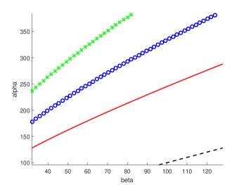
Figure 1: Visualization of $I$, $I_{2}$, $I_{sdp}$ when $k=6$: (a) the solid line represents $I(\alpha,\beta)=1$, (b) the circled line represents $I_{2}(\alpha,\beta)=1$, and (c) the x-marked line represents $I_{sdp}(\alpha,\beta)=1$. The dashed black line is the graph of $\alpha=\beta$.

We note that

$$I(\alpha,\beta)=\max_{t\geq 0}\frac{1}{2^{k-1}}\left(\alpha(1-e^{-(k-1)t})+\beta(1-e^{(k-1)t})\right),$$

hence $I(\alpha,\beta)<I_{2}(\alpha,\beta)$ for any $\alpha>\beta>0$. Figure 1 shows the relations between $I$, $I_{2}$ and $I_{sdp}$ for $k=6$.

Theorem 3 and the discussion above implies that the truncate-and-relax algorithm fails with probability $1-o_{n}(1)$ if $I_{2}(\alpha,\beta)>1$. We conjecture that this is the correct threshold of the performance of the algorithm. In future work, we will attempt to prove this conjecture by improving the matrix concentration bound as discussed above.

Conjecture 1.2.

If $I_{2}(\alpha,\beta)>1$, then $\widehat{\Sigma}(\mathcal{H})=\sigma\sigma^{T}$ with probability $1-o_{n}(1)$.

2 Maximum-likelihood estimator

Recall that $\widehat{\sigma}_{MLE}(H)$ is a maximizer of the likelihood probability $\operatorname*{\mathbb{P}}(\mathcal{H}=H|\sigma=x)$ (ties are broken arbitrarily). Let $f_{H}(x)=\log\operatorname*{\mathbb{P}}(\mathcal{H}=H|\sigma=x)$ for $x\in\{\pm 1\}^{V}$.

For brevity, let us first introduce a few notations. Let $x\in\{\pm 1\}^{V}$. Let $x^{\mathchoice{\mathbin{\ooalign{$\displaystyle=$\crcr$\displaystyle\ovoid$}}}{\mathbin{\ooalign{$\textstyle=$\crcr$\textstyle\ovoid$}}}{\mathbin{\ooalign{$\scriptstyle=$\crcr$\scriptstyle\ovoid$}}}{\mathbin{\ooalign{$\scriptscriptstyle=$\crcr$\scriptscriptstyle\ovoid$}}}k}$ be a vector in $\{0,1\}^{\binom{V}{k}}$ where

$$(x^{\mathchoice{\mathbin{\ooalign{$\displaystyle=$\crcr$\displaystyle\ovoid$}}}{\mathbin{\ooalign{$\textstyle=$\crcr$\textstyle\ovoid$}}}{\mathbin{\ooalign{$\scriptstyle=$\crcr$\scriptstyle\ovoid$}}}{\mathbin{\ooalign{$\scriptscriptstyle=$\crcr$\scriptscriptstyle\ovoid$}}}k})_{e}=\begin{cases}1&\text{if $x_{e_{1}}=x_{e_{2}}=\cdots=x_{e_{k}}$}\\ 0&\text{otherwise}\end{cases}$$

for each $e=\{e_{1},\cdots,e_{k}\}\subseteq V$. Let $H$ be a $k$-uniform hypergraph on the vertex set $V$ with the edge set $E(H)$. Let $A_{H}$ be the vector in $\{0,1\}^{\binom{V}{k}}$ such that

$$(A_{H})_{e}=\begin{cases}1&\text{if $e\in E(H)$}\\ 0&\text{otherwise}\end{cases}$$

for each $e\in\binom{V}{k}$. Note that

$$\langle A_{H},x^{\mathchoice{\mathbin{\ooalign{$\displaystyle=$\crcr$\displaystyle\ovoid$}}}{\mathbin{\ooalign{$\textstyle=$\crcr$\textstyle\ovoid$}}}{\mathbin{\ooalign{$\scriptstyle=$\crcr$\scriptstyle\ovoid$}}}{\mathbin{\ooalign{$\scriptscriptstyle=$\crcr$\scriptscriptstyle\ovoid$}}}k}\rangle = \sum_{e\in\binom{V}{k}}(A_{H})_{e}(x^{\mathchoice{\mathbin{\ooalign{$\displaystyle=$\crcr$\displaystyle\ovoid$}}}{\mathbin{\ooalign{$\textstyle=$\crcr$\textstyle\ovoid$}}}{\mathbin{\ooalign{$\scriptstyle=$\crcr$\scriptstyle\ovoid$}}}{\mathbin{\ooalign{$\scriptscriptstyle=$\crcr$\scriptscriptstyle\ovoid$}}}k})_{e}$$

$$= \sum_{e\in E(H)}\mathbf{1}\{\text{$e$ is in-cluster with respect to $x$}\}.$$

Hence, $\langle A_{H},x^{\mathchoice{\mathbin{\ooalign{$\displaystyle=$\crcr$\displaystyle\ovoid$}}}{\mathbin{\ooalign{$\textstyle=$\crcr$\textstyle\ovoid$}}}{\mathbin{\ooalign{$\scriptstyle=$\crcr$\scriptstyle\ovoid$}}}{\mathbin{\ooalign{$\scriptscriptstyle=$\crcr$\scriptscriptstyle\ovoid$}}}k}\rangle$ is equal to the number of in-cluster edges in $H$ with respect to the partition $x$.

The ML estimator tries to find the “best” partition $x\in\{\pm 1\}^{V}$ with equal number of $1$’s and $-1$’s. Intuitively, if $p>q$, i.e., in-cluster edges appears more likely than cross-cluster edges (we call such case assortative), then the best partition will correspond to $x$ which maximizes the number of in-cluster edges w.r.t. $x$. On the other hand, if $p<q$ (we call such case disassortative) then the best partition will corresponds to the minimizer, respectively. The following proposition confirms this intuition. We defer the proof to Section B.1 in the appendix.

Proposition 1.

The ML estimator $\widehat{\sigma}_{MLE}(H)$ is the maximizer (minimizer, respectively) of $\langle A_{H},x^{\mathchoice{\mathbin{\ooalign{$\displaystyle=$\crcr$\displaystyle\ovoid$}}}{\mathbin{\ooalign{$\textstyle=$\crcr$\textstyle\ovoid$}}}{\mathbin{\ooalign{$\scriptstyle=$\crcr$\scriptstyle\ovoid$}}}{\mathbin{\ooalign{$\scriptscriptstyle=$\crcr$\scriptscriptstyle\ovoid$}}}k}\rangle$ if $p>q$ (if $p<q$, respectively) over all $x\in\{\pm 1\}^{V}$ such that $\mathbf{1}^{T}x=0$.

3 Sharp phase transition in $\mathsf{HSBM}(n,p,q;k)$

In this section, we prove Theorem 1. The techniques we use can be seen as a hypergraph extension of the techniques used in [ABH16].

Informally, we are going to argue that the event for the ground truth $\sigma$ being the best guess (i.e. $\sigma$ is the global optimum of the likelihood function) can be approximately decomposed into the events that $\sigma$ is unimprovable by flipping the label of $v$ for $v\in V$. This type of phenomenon was called local-to-global amplification in [Abb18] which seems to hold for more general classes of the graphical model.

Let $p_{fail}$ be the probability that the ML estimator fails to recover the hidden partition, i.e.,

$$p_{fail}=\operatorname*{\mathbb{P}}_{(\sigma,\mathcal{H})\sim\mathsf{HSBM}(n,p,q;k)}\left(\widehat{\sigma}_{MLE}(\mathcal{H})\not\in\{\sigma,-\sigma\}\right).$$

As we have seen in the previous section, the ML estimator $\widehat{\sigma}_{MLE}(H)$ is a maximizer of $\langle A_{H},x^{\mathchoice{\mathbin{\ooalign{$\displaystyle=$\crcr$\displaystyle\ovoid$}}}{\mathbin{\ooalign{$\textstyle=$\crcr$\textstyle\ovoid$}}}{\mathbin{\ooalign{$\scriptstyle=$\crcr$\scriptstyle\ovoid$}}}{\mathbin{\ooalign{$\scriptscriptstyle=$\crcr$\scriptscriptstyle\ovoid$}}}k}\rangle$ over the choices of $x\in\{\pm 1\}^{V}$ such that $\mathbf{1}^{T}x=0$. Thus, $p_{fail}$ is equal to the probability that $\langle A_{\mathcal{H}},x^{\mathchoice{\mathbin{\ooalign{$\displaystyle=$\crcr$\displaystyle\ovoid$}}}{\mathbin{\ooalign{$\textstyle=$\crcr$\textstyle\ovoid$}}}{\mathbin{\ooalign{$\scriptstyle=$\crcr$\scriptstyle\ovoid$}}}{\mathbin{\ooalign{$\scriptscriptstyle=$\crcr$\scriptscriptstyle\ovoid$}}}k}\rangle\geq\langle A_{\mathcal{H}},\sigma^{\mathchoice{\mathbin{\ooalign{$\displaystyle=$\crcr$\displaystyle\ovoid$}}}{\mathbin{\ooalign{$\textstyle=$\crcr$\textstyle\ovoid$}}}{\mathbin{\ooalign{$\scriptstyle=$\crcr$\scriptstyle\ovoid$}}}{\mathbin{\ooalign{$\scriptscriptstyle=$\crcr$\scriptscriptstyle\ovoid$}}}k}\rangle$ happens for some $x\not\in\{\sigma,-\sigma\}$ satisfying the balance condition $\mathbf{1}^{T}x=0$.

3.1 Lower bound

We first prove the impossibility part of Theorem 1. For concreteness, we focus on the assortative case, i.e., $p>q$ but the proof can be easily adapted for the disassortative case.

Before we prove the lower bound, let us consider the usual stochastic block model for graphs which corresponds to $k=2$ in order to explain the intuition of the proof. Given a sample $G$, partition $\sigma$ and a vertex $v\in V$, let us define the in-degree of $v$ as

$$\mathrm{indeg}_{G,\sigma}(v)=\#(vw\in E(G):\sigma_{v}=\sigma_{w}),$$

and the out-degree of $v$ as

$$\mathrm{outdeg}_{G,\sigma}(v;\sigma)=\#(vw\in E(G):\sigma_{v}\neq\sigma_{w}).$$

We will omit the subscript $G,\sigma$ if the context is clear.

Suppose that there are vertices $v$ and $w$ from different clusters such that the in-degree of each vertex is smaller than the out-degree of each vertex. In this case, swapping the label of $v$ and $w$ will yield a new balanced partition with greater number of in-cluster edges, hence the ML estimator will fail to recover $\sigma$. Now, suppose that

$$\operatorname*{\mathbb{P}}(\mathrm{indeg}(v)<\mathrm{outdeg}(v))=\omega(n^{-1})$$

for all $v$. If those events were independent, we would get

$$1-\operatorname*{\mathbb{P}}(\exists v\text{ s.t. }\sigma_{v}=1,\mathrm{indeg}(v)<\mathrm{outdeg}(v)) = \prod_{v:\sigma_{v}=1}\left(1-\operatorname*{\mathbb{P}}(\mathrm{indeg}(v)<\mathrm{outdeg}(v))\right)$$

$$\leq (1-\omega(n^{-1}))^{n/2}\leq e^{-\omega(1)},$$

and vise versa for $w$. It would imply that there is a “bad” pair $(v,w)$ with probability $1-o_{n}(1)$ hence the ML estimator fails with probability $1-o_{n}(1)$. We remark that this argument is not mathematically because the in-degrees of vertex $v$ and $w$ (as well as out-degrees of them) are not independent as they share a variable indicating whether $\{v,w\}$ is an edge or not. However, we can overcome it by conditioning on highly probable event which makes those events independent, as in [ABH16].

We extend the definitions of in-degree and out-degree for the $k$-HSBM as

$$\mathrm{indeg}_{H,\sigma}(v) = \#(e\in E(H):v\in e,\text{ $e$ is in-cluster w.r.t. $\sigma$}),$$

$$\mathrm{outdeg}_{H,\sigma}(v) = \#(e\in E(H):v\in e,\text{ $e$ is cross-cluster but $e\setminus\{v\}$ is in-cluster w.r.t. $\sigma$}).$$

Observe that they coincide with the corresponding definition for the usual SBM ($k=2$). We note that the sum of in-degree and out-degree is not equal to the degree of $v$, the number of hyperedges in $H$ containing $v$ when $k\geq 3$. We extended those definitions in this way because any edge $e$ which is neither in-cluster nor cross-cluster but $e\setminus\{v\}$ is in-cluster does not contribute on $\langle A_{\mathcal{H}},x^{\mathchoice{\mathbin{\ooalign{$\displaystyle=$\crcr$\displaystyle\ovoid$}}}{\mathbin{\ooalign{$\textstyle=$\crcr$\textstyle\ovoid$}}}{\mathbin{\ooalign{$\scriptstyle=$\crcr$\scriptstyle\ovoid$}}}{\mathbin{\ooalign{$\scriptscriptstyle=$\crcr$\scriptscriptstyle\ovoid$}}}k}\rangle$ when we flip the sign of the label of $v$.

Now, note that the in-degree and the out-degree of $v$ are independent binomial random variables with different parameters. To estimate the probability

$$\operatorname*{\mathbb{P}}\left(\mathrm{indeg}(v)-\mathrm{outdeg}(v)<0\right),$$

we provide a tight estimate for the tail probability of a weighted sum of independent binomial variables in Section A. Precisely we prove that

$$\operatorname*{\mathbb{P}}(\mathrm{indeg}(v)-\mathrm{outdeg}(v)<-\delta\log n)=n^{-I(\alpha,\beta)+o_{n}(1)}$$

as long as $\delta=\delta(n)$ vanishes as $n$ grows, where

$$I(\alpha,\beta)=\frac{1}{2^{k-1}}\left(\sqrt{\alpha}-\sqrt{\beta}\right)^{2}.$$

As we discussed, if $I(\alpha,\beta)<1$ then the tail probability is of order $\omega(n^{-1})$ and it implies that the ML estimator fails with probability $1-o_{n}(1)$.

Theorem 4.

Let $I(\alpha,\beta)=\frac{1}{2^{k-1}}(\sqrt{\alpha}-\sqrt{\beta})^{2}$. If $I(\alpha,\beta)<1$, then $p_{fail}=1-o_{n}(1)$.

Proof.

Let $A=\{v\in V:\sigma_{v}=+1\}$ and $B=V\setminus A$. For $a\in A$ and $b\in B$, let us define $\sigma^{(ab)}$ to be the vector obtained by flipping the signs of $\sigma_{a}$ and $\sigma_{b}$. By definition, $\sigma^{(ab)}$ is balanced. We are going to prove that with high probability there exist $a\in A$ and $b\in B$ such that $\langle A_{\mathcal{H}},\sigma^{\mathchoice{\mathbin{\ooalign{$\displaystyle=$\crcr$\displaystyle\ovoid$}}}{\mathbin{\ooalign{$\textstyle=$\crcr$\textstyle\ovoid$}}}{\mathbin{\ooalign{$\scriptstyle=$\crcr$\scriptstyle\ovoid$}}}{\mathbin{\ooalign{$\scriptscriptstyle=$\crcr$\scriptscriptstyle\ovoid$}}}k}\rangle\leq\langle A_{\mathcal{H}},(\sigma^{(ab)})^{\mathchoice{\mathbin{\ooalign{$\displaystyle=$\crcr$\displaystyle\ovoid$}}}{\mathbin{\ooalign{$\textstyle=$\crcr$\textstyle\ovoid$}}}{\mathbin{\ooalign{$\scriptstyle=$\crcr$\scriptstyle\ovoid$}}}{\mathbin{\ooalign{$\scriptscriptstyle=$\crcr$\scriptscriptstyle\ovoid$}}}k}\rangle$. For simplicity, let $\Sigma=\sigma^{\mathchoice{\mathbin{\ooalign{$\displaystyle=$\crcr$\displaystyle\ovoid$}}}{\mathbin{\ooalign{$\textstyle=$\crcr$\textstyle\ovoid$}}}{\mathbin{\ooalign{$\scriptstyle=$\crcr$\scriptstyle\ovoid$}}}{\mathbin{\ooalign{$\scriptscriptstyle=$\crcr$\scriptscriptstyle\ovoid$}}}k}$ and $\Sigma^{(ab)}=(\sigma^{(ab)})^{\mathchoice{\mathbin{\ooalign{$\displaystyle=$\crcr$\displaystyle\ovoid$}}}{\mathbin{\ooalign{$\textstyle=$\crcr$\textstyle\ovoid$}}}{\mathbin{\ooalign{$\scriptstyle=$\crcr$\scriptstyle\ovoid$}}}{\mathbin{\ooalign{$\scriptscriptstyle=$\crcr$\scriptscriptstyle\ovoid$}}}k}$.

Note that

$$\langle A_{\mathcal{H}},\Sigma\rangle-\langle A_{\mathcal{H}},\Sigma^{(ab)}\rangle = \left(\mathrm{indeg}_{\mathcal{H},\sigma}(a)-\mathrm{outdeg}_{\mathcal{H},\sigma}(a)\right)$$

$$+\left(\mathrm{indeg}_{\mathcal{H},\sigma}(b)-\mathrm{outdeg}_{\mathcal{H},\sigma}(b)\right).$$

For $v\in V$, let $E_{v}$ be the event such that

$$\mathrm{indeg}_{\mathcal{H},\sigma}(v)-\mathrm{outdeg}_{\mathcal{H},\sigma}(v)\leq 0$$

holds. Then, $E_{a}\cap E_{b}$ implies that $\langle A_{\mathcal{H}},\Sigma\rangle-\langle A_{\mathcal{H}},\Sigma^{(ab)}\rangle\leq 0$. Hence

$$p_{fail}=\operatorname*{\mathbb{P}}\left(\exists a\in A,b\in B:\langle A_{\mathcal{H}},\Sigma\rangle-\langle A_{\mathcal{H}},\Sigma^{(ab)}\rangle\right)\geq\operatorname*{\mathbb{P}}\left(\bigcup_{a\in A}E_{a}\cap\bigcup_{b\in B}E_{b}\right).$$

We recall that if $E_{v}$ for $v\in V$ were mutually independent, we can exactly express the right-hand side as

$$\left(1-\prod_{a\in A}\operatorname*{\mathbb{P}}(\neg E_{a})\right)\left(1-\prod_{b\in B}\operatorname*{\mathbb{P}}(\neg E_{b})\right)$$

but unfortunately it is not the case. To see this, let us fix $a\in A$ and $a^{\prime}\in A$. Then, we have

$$\mathrm{indeg}(a)-\mathrm{outdeg}(a) = \sum_{e\ni a:e\subseteq A}(A_{\mathcal{H}})_{e}-\sum_{e\ni a:e\cap A=\{a\}}(A_{\mathcal{H}})_{e},\text{ and}$$

$$\mathrm{indeg}(a^{\prime})-\mathrm{outdeg}(a^{\prime}) = \sum_{e\ni a^{\prime}:e\subseteq A}(A_{\mathcal{H}})_{e}-\sum_{e\ni a^{\prime}:e\cap A=\{a^{\prime}\}}(A_{\mathcal{H}})_{e}.$$

They share variables $(A_{\mathcal{H}})_{e}$ for $e$ satisfying $\{a,a^{\prime}\}\subseteq e\subseteq A$. The expected contribution of those variables is $p\binom{|A|-2}{k-2}=o_{n}(1)$, so we may expect

$$\operatorname*{\mathbb{P}}(E_{a}\cup E_{a^{\prime}})\approx 1-\operatorname*{\mathbb{P}}(\neg E_{a})\operatorname*{\mathbb{P}}(\neg E_{a^{\prime}}).$$

In the similar spirit, we are going to prove that for an appropriate choice of $U\subseteq V$, the events $\{E_{a}\}_{a\in U\cap A}$ and $\{E_{b}\}_{b\in U\cap B}$ are approximately independent, so

$$p_{fail} \geq \operatorname*{\mathbb{P}}\left(\bigcup_{a\in A\cap U}E_{a}\cap\bigcup_{b\in B\cap U}E_{b}\right)$$

$$\approx \left(1-\prod_{a\in A\cap U}\operatorname*{\mathbb{P}}(\neg E_{a})\right)\left(1-\prod_{b\in B\cap U}\operatorname*{\mathbb{P}}(\neg E_{b})\right).$$

Together with the tight estimate on $\operatorname*{\mathbb{P}}(E_{v})$, it would give us a good lower bound on $p_{fail}$.

Let $U\subseteq V$ be a set of size $\gamma n$ where $|U\cap A|=|U\cap B|$. We will choose $\gamma=\gamma(n)$ later to be poly-logarithmically decaying function in $n$. Let $\mathcal{S}$ be the set of $e\in\binom{V}{k}$ such that $e$ contains at least two vertices in $U$. We would like to condition on the values of $\{(A_{\mathcal{H}})_{e}\}_{e\in\mathcal{S}}$, which captures all dependency occurring among $E_{v}$’s for $v\in U$.

Let $\delta=\delta(n)$ be a positive number depending on $n$ which we will choose later, and let $F$ be the event that the inequality

$$\max_{v\in U}\sum_{e\in\mathcal{S}:e\ni v}(A_{\mathcal{H}})_{e}\leq\delta\log n$$

holds. For each $a\in A\cap U$, let $E_{a}^{\prime}$ be the event that the inequality

$$\sum_{e\subseteq A:e\cap U=\{a\}}(A_{\mathcal{H}})_{e}-\sum_{\begin{subarray}{c}e:e\cap U=\{a\}\\ e\setminus\{a\}\subseteq B\end{subarray}}(A_{\mathcal{H}})_{e}\leq-\delta\log n$$

is satisfied. We claim that $E_{a}^{\prime}\cap F\subseteq E_{a}$. It follows from the direct calculation, as if we assume $E_{a}^{\prime}\cap F$, then

$$\mathrm{indeg}(v)-\mathrm{outdeg}(v) = \sum_{e\ni a:e\subseteq A}(A_{\mathcal{H}})_{e}-\sum_{e\ni a:e\cap A=\{a\}}(A_{\mathcal{H}})_{e}$$

$$\leq \sum_{e\subseteq A:e\cap U=\{a\}}(A_{\mathcal{H}})_{e}-\sum_{\begin{subarray}{c}e:e\cap U=\{a\}\\ e\setminus\{a\}\subseteq B\end{subarray}}(A_{\mathcal{H}})_{e}+\sum_{e\in\mathcal{S}:e\ni a}(A_{\mathcal{H}})_{e}$$

$$\leq \sum_{e\subseteq A:e\cap U=\{a\}}(A_{\mathcal{H}})_{e}-\sum_{\begin{subarray}{c}e:e\cap U=\{a\}\\ e\setminus\{a\}\subseteq B\end{subarray}}(A_{\mathcal{H}})_{e}+\delta\log n$$

$$\leq 0.$$

We get

$$p_{fail}\geq\operatorname*{\mathbb{P}}\left(\bigcup_{a\in A\cap U}E_{a}\cap\bigcup_{b\in B\cap U}E_{b}\right)\geq\operatorname*{\mathbb{P}}\left(\bigcup_{a\in A\cap U}E_{a}^{\prime}\cap\bigcup_{b\in B\cap U}E_{b}^{\prime}\middle|F\right)\operatorname*{\mathbb{P}}(F).$$

Note that $E_{v}^{\prime}$ only depends on the set of variables $\{(A_{\mathcal{H}})_{e}:e\cap U=\{v\}\}$, which are mutually disjoint for $v\in U$. Also, $\{(A_{\mathcal{H}})_{e}:e\in\mathcal{S}\}$ is disjoint with any of those sets of variables. Hence, events $F$ and $\{E_{v}^{\prime}\}_{v\in U}$ are mutually independent, and we get

$$\operatorname*{\mathbb{P}}\left(\bigcup_{a\in A\cap U}E_{a}^{\prime}\cap\bigcup_{b\in B\cap U}E_{b}^{\prime}\middle|F\right) = \operatorname*{\mathbb{P}}\left(\bigcup_{a\in A\cap U}E_{a}^{\prime}\right)\operatorname*{\mathbb{P}}\left(\bigcup_{b\in B\cap U}E_{b}^{\prime}\right)$$

$$= \left(1-\prod_{a\in A\cap U}\operatorname*{\mathbb{P}}(\neg E_{a}^{\prime})\right)\left(1-\prod_{b\in B\cap U}\operatorname*{\mathbb{P}}(\neg E_{b}^{\prime})\right)$$

We claim that

$$\prod_{a\in A\cap U}\operatorname*{\mathbb{P}}(\neg E_{a}^{\prime})=o_{n}(1),\quad\prod_{b\in B\cap U}\operatorname*{\mathbb{P}}(\neg E_{b}^{\prime})=o_{n}(1)\quad\text{and}\quad\operatorname*{\mathbb{P}}(\neg F)=o_{n}(1),$$

for appropriate choice of $\gamma$ and $\delta$. This immediately implies that $p_{fail}=1-o_{n}(1)$ as desired.

Let us first prove $\operatorname*{\mathbb{P}}(\neg F)=o_{n}(1)$. Let $X_{v}$ be the random variable defined as

$$X_{v}:=\sum_{e\in\mathcal{S}:e\ni v}(A_{\mathcal{H}})_{e},$$

for $v\in U$. We have

$$\operatorname*{\mathbb{P}}(\neg F)=\operatorname*{\mathbb{P}}(\exists v\in U:X_{v}>\delta\log n)\leq\sum_{v\in U}\operatorname*{\mathbb{P}}(X_{v}>\delta\log n)$$

by a union bound. Note that

$$\operatorname*{\mathbb{E}}X_{v} \leq \max(p,q)\#(e:e\ni v,|e\cap U|\geq 2)$$

$$= \frac{\max(\alpha,\beta)\log n}{\binom{n-1}{k-1}}\left(\binom{n-1}{k-1}-\binom{n-|U|}{k-1}\right)$$

$$\lesssim \left(1-(1-\gamma)^{k-1}\right)\log n=\Theta(\gamma\log n).$$

Using a standard Chernoff bound, we get the following lemma. For completeness, we include the proof in the appendix (Section A.1).

Lemma 1.

Let $X$ be a sum of independent Bernoulli variables such that $\operatorname*{\mathbb{E}}X=\Theta(\gamma\log n)$ where $\gamma=o_{n}(\log^{-1}n)$. Let $\delta$ be a positive number which decays to 0 as $n$ grows, with $\delta=\omega_{n}(\log^{-1}n)$. Then,

$$\operatorname*{\mathbb{P}}\left(X>\delta\log n\right)\leq n^{-\delta\log\frac{\delta}{\gamma}+o_{n}(1)}.$$

Letting $\gamma=\log^{-3}n$ and $\delta=(\log\log n)^{-1}$, we get

$$\delta\log\frac{\delta}{\gamma}=\frac{3\log\log n-\log\log\log n}{\log\log n}=3-o_{n}(1)$$

and so $\operatorname*{\mathbb{P}}(\neg F)=n^{-3+o_{n}(1)}=o_{n}(1)$.

Now, we would like to prove that

$$\prod_{a\in A\cap U}\operatorname*{\mathbb{P}}(\neg E_{a}^{\prime})=o_{n}(1)\quad\text{and}\quad\prod_{b\in B\cap U}\operatorname*{\mathbb{P}}(\neg E_{b}^{\prime})=o_{n}(1)$$

by showing that

$$\operatorname*{\mathbb{P}}(E_{v}^{\prime})\geq n^{-I(\alpha,\beta)+o_{n}(1)}\quad\text{where }I(\alpha,\beta)=\frac{1}{2^{k-1}}(\sqrt{\alpha}-\sqrt{\beta})^{2}$$

for any $v\in U$. This implies that

$$\prod_{a\in A\cap U}\operatorname*{\mathbb{P}}(\neg E_{a}^{\prime}) \leq \left(1-n^{-I(\alpha,\beta)+o_{n}(1)}\right)^{\gamma n/2}$$

$$\leq \exp\left(-\frac{\gamma}{2}n^{1-I(\alpha,\beta)+o_{n}(1)}\right),$$

and since we assumed that $I(\alpha,\beta)<1$ and $\gamma=\log^{-3}n$, we get

$$\prod_{a\in A\cap U}\operatorname*{\mathbb{P}}(\neg E_{a}^{\prime})\leq e^{-\frac{n^{1-I(\alpha,\beta)}}{\log^{3}n}}=o_{n}(1),$$

and similarly $\prod_{b\in B\cap U}\operatorname*{\mathbb{P}}(\neg E_{b}^{\prime})=o_{n}(1)$ as desired.

To estimate the probability that $E_{a}^{\prime}$ happens, let $Y_{a}$ and $Z_{a}$ be random variables defined as

$$Y_{a}=\sum_{e\subseteq A:e\cap U=\{a\}}(A_{\mathcal{H}})_{e}\quad\text{and}\quad Z_{a}=\sum_{\begin{subarray}{c}e:e\cap U=\{a\}\\ e\setminus\{a\}\subseteq B\end{subarray}}(A_{\mathcal{H}})_{e}.$$

Recall that $E_{a}^{\prime}$ is the event that $Y_{a}-Z_{a}\leq-\delta\log n$ holds.

Lemma 2.

Let $Y$ be a binomial random variable from $\mathrm{Bin}(N,p)$ and $Z$ be a binomial random variable from $\mathrm{Bin}(N,q)$ where $N=\left(\frac{1}{2^{k-1}}\pm o_{n}(1)\right)\binom{n-1}{k-1}$, $p=\frac{\alpha\log n}{\binom{n-1}{k-1}}$ and $q=\frac{\beta\log n}{\binom{n-1}{k-1}}$. Let $I(\alpha,\beta)=\frac{1}{2^{k-1}}(\sqrt{\alpha}-\sqrt{\beta})^{2}$ and let $\delta$ be a positive number vanishing as $n$ grows. Then,

$$\operatorname*{\mathbb{P}}(Y-Z\leq-\delta\log n)=n^{-I(\alpha,\beta)+o_{n}(1)}.$$

In fact, we derive a generic tail bound for weighted sum of binomial random variables (Theorem 10) in Section A of the appendix. Lemma 2 is a direct corollary of Theorem 10 and we defer the proof to Section A.2. ∎

3.2 Upper bound

We are going to use a union bound to prove the upper bound. Let $x$ and $\sigma$ be vectors in $\{-1,+1\}^{V}$. The Hamming distance between $x$ and $\sigma$ (denoted $d(x,\sigma)$) is defined as the number of $v\in V$ such that $x_{v}\neq\sigma_{v}$. Note that if $x$ and $\sigma$ are balanced, then

$$d(x,\sigma) = \#(v\in V:x_{v}=1,\sigma_{v}=-1)+\#(v\in V:x_{v}=-1,\sigma_{v}=1)$$

$$= \#(v\in V:x_{v}=1)+\#(v\in V:\sigma_{v}=1)-2\#(v\in V:x_{v}=\sigma_{v}=1)$$

$$= n-2\#(v\in V:x_{v}=\sigma_{v}=1),$$

hence $d(x,\sigma)$ is even.

Let us fix $\sigma$ and let $\mathcal{H}$ be a $k$-uniform random hypergraph generated by the model under the ground truth $\sigma$. We note that the distribution of the random variable $\langle A_{\mathcal{H}},x^{\mathchoice{\mathbin{\ooalign{$\displaystyle=$\crcr$\displaystyle\ovoid$}}}{\mathbin{\ooalign{$\textstyle=$\crcr$\textstyle\ovoid$}}}{\mathbin{\ooalign{$\scriptstyle=$\crcr$\scriptstyle\ovoid$}}}{\mathbin{\ooalign{$\scriptscriptstyle=$\crcr$\scriptscriptstyle\ovoid$}}}k}-\sigma^{\mathchoice{\mathbin{\ooalign{$\displaystyle=$\crcr$\displaystyle\ovoid$}}}{\mathbin{\ooalign{$\textstyle=$\crcr$\textstyle\ovoid$}}}{\mathbin{\ooalign{$\scriptstyle=$\crcr$\scriptstyle\ovoid$}}}{\mathbin{\ooalign{$\scriptscriptstyle=$\crcr$\scriptscriptstyle\ovoid$}}}k}\rangle$ is invariant under the permutation of $V$ preserving $\sigma$, hence it only depends on $d(x,\sigma)$. Hence, there is a quantity $p_{fail}^{(d)}$ which satisfies

$$p_{fail}^{(d)}=\operatorname*{\mathbb{P}}(\langle A_{\mathcal{H}},x^{\mathchoice{\mathbin{\ooalign{$\displaystyle=$\crcr$\displaystyle\ovoid$}}}{\mathbin{\ooalign{$\textstyle=$\crcr$\textstyle\ovoid$}}}{\mathbin{\ooalign{$\scriptstyle=$\crcr$\scriptstyle\ovoid$}}}{\mathbin{\ooalign{$\scriptscriptstyle=$\crcr$\scriptscriptstyle\ovoid$}}}k}-\sigma^{\mathchoice{\mathbin{\ooalign{$\displaystyle=$\crcr$\displaystyle\ovoid$}}}{\mathbin{\ooalign{$\textstyle=$\crcr$\textstyle\ovoid$}}}{\mathbin{\ooalign{$\scriptstyle=$\crcr$\scriptstyle\ovoid$}}}{\mathbin{\ooalign{$\scriptscriptstyle=$\crcr$\scriptscriptstyle\ovoid$}}}k}\rangle\geq 0)$$

for any $x$ with $d(x,\sigma)=d$. Moreover, $p_{fail}^{(d)}=p_{fail}^{(n-d)}$ since our model is invariant under a global sign flip.

Recall that the ML estimator fails to recover $\sigma$ if and only if

$$\langle A_{\mathcal{H}},x^{\mathchoice{\mathbin{\ooalign{$\displaystyle=$\crcr$\displaystyle\ovoid$}}}{\mathbin{\ooalign{$\textstyle=$\crcr$\textstyle\ovoid$}}}{\mathbin{\ooalign{$\scriptstyle=$\crcr$\scriptstyle\ovoid$}}}{\mathbin{\ooalign{$\scriptscriptstyle=$\crcr$\scriptscriptstyle\ovoid$}}}k}\rangle\geq\langle A_{\mathcal{H}},\sigma^{\mathchoice{\mathbin{\ooalign{$\displaystyle=$\crcr$\displaystyle\ovoid$}}}{\mathbin{\ooalign{$\textstyle=$\crcr$\textstyle\ovoid$}}}{\mathbin{\ooalign{$\scriptstyle=$\crcr$\scriptstyle\ovoid$}}}{\mathbin{\ooalign{$\scriptscriptstyle=$\crcr$\scriptscriptstyle\ovoid$}}}k}\rangle$$

for some balanced $x\in\{\pm 1\}^{V}$ which is neither $\sigma$ nor $-\sigma$. We remark that we count the equality as a failure, which will only make $p_{fail}$ larger. By union bound, we have

$$p_{fail} \leq \sum_{\begin{subarray}{c}x\in\{\pm 1\}^{V}:\mathbf{1}^{T}x=0,\\ 1\leq d(x,\sigma)\leq n-1\end{subarray}}\operatorname*{\mathbb{P}}(\langle A_{\mathcal{H}},x^{\mathchoice{\mathbin{\ooalign{$\displaystyle=$\crcr$\displaystyle\ovoid$}}}{\mathbin{\ooalign{$\textstyle=$\crcr$\textstyle\ovoid$}}}{\mathbin{\ooalign{$\scriptstyle=$\crcr$\scriptstyle\ovoid$}}}{\mathbin{\ooalign{$\scriptscriptstyle=$\crcr$\scriptscriptstyle\ovoid$}}}k}-\sigma^{\mathchoice{\mathbin{\ooalign{$\displaystyle=$\crcr$\displaystyle\ovoid$}}}{\mathbin{\ooalign{$\textstyle=$\crcr$\textstyle\ovoid$}}}{\mathbin{\ooalign{$\scriptstyle=$\crcr$\scriptstyle\ovoid$}}}{\mathbin{\ooalign{$\scriptscriptstyle=$\crcr$\scriptscriptstyle\ovoid$}}}k}\rangle\geq 0)$$

$$\leq 2\sum_{\begin{subarray}{c}d:1\leq d\leq\frac{n}{2}\\ d\text{ is even}\end{subarray}}p_{fail}^{(d)}\cdot\#(x\in\{\pm 1\}^{V}:\mathbf{1}^{T}x=0,d(x,\sigma)=d).$$

We note that there is a one-to-one correspondence between a balanced $x$ and a pair of sets $(U_{+},U_{-})$ where

$$U_{+} = \{v:x_{v}=-1,\sigma_{v}=1\}\subseteq\{v:\sigma_{v}=+1\}$$

$$U_{-} = \{v:x_{v}=1,\sigma_{v}=-1\}\subseteq\{v:\sigma_{v}=-1\},$$

and we must have $d(x,\sigma)=2|U_{+}|=2|U_{-}|$ since $x$ is balanced. Hence, the number of balanced $x$’s with $d(x,\sigma)=d$ is equal to $\binom{n/2}{d/2}^{2}$. We have

$$p_{fail}\leq 2\sum_{\begin{subarray}{c}d:1\leq d\leq\frac{n}{2}\\ d\text{ is even}\end{subarray}}\binom{n/2}{d/2}^{2}p_{fail}^{(d)}.$$

Now, let us formally state the main result of this section.

Theorem 5.

Suppose that $I(\alpha,\beta)>1$. Then,

$$p_{fail}\leq n^{-\frac{I(\alpha,\beta)-1}{2}+o_{n}(1)}$$

and it implies that $p_{fail}=o_{n}(1)$.

Proof.

Let $d$ be even number in between 1 and $\frac{n}{2}$. Choose any balanced $x$ with $d(\sigma,x)=d$, and let $X_{d}$ be

$$X_{d}:=\langle A_{\mathcal{H}},x^{\mathchoice{\mathbin{\ooalign{$\displaystyle=$\crcr$\displaystyle\ovoid$}}}{\mathbin{\ooalign{$\textstyle=$\crcr$\textstyle\ovoid$}}}{\mathbin{\ooalign{$\scriptstyle=$\crcr$\scriptstyle\ovoid$}}}{\mathbin{\ooalign{$\scriptscriptstyle=$\crcr$\scriptscriptstyle\ovoid$}}}k}-\sigma^{\mathchoice{\mathbin{\ooalign{$\displaystyle=$\crcr$\displaystyle\ovoid$}}}{\mathbin{\ooalign{$\textstyle=$\crcr$\textstyle\ovoid$}}}{\mathbin{\ooalign{$\scriptstyle=$\crcr$\scriptstyle\ovoid$}}}{\mathbin{\ooalign{$\scriptscriptstyle=$\crcr$\scriptscriptstyle\ovoid$}}}k}\rangle=\sum_{e\in\binom{V}{k}}(A_{\mathcal{H}})_{e}\left(x^{\mathchoice{\mathbin{\ooalign{$\displaystyle=$\crcr$\displaystyle\ovoid$}}}{\mathbin{\ooalign{$\textstyle=$\crcr$\textstyle\ovoid$}}}{\mathbin{\ooalign{$\scriptstyle=$\crcr$\scriptstyle\ovoid$}}}{\mathbin{\ooalign{$\scriptscriptstyle=$\crcr$\scriptscriptstyle\ovoid$}}}k}-\sigma^{\mathchoice{\mathbin{\ooalign{$\displaystyle=$\crcr$\displaystyle\ovoid$}}}{\mathbin{\ooalign{$\textstyle=$\crcr$\textstyle\ovoid$}}}{\mathbin{\ooalign{$\scriptstyle=$\crcr$\scriptstyle\ovoid$}}}{\mathbin{\ooalign{$\scriptscriptstyle=$\crcr$\scriptscriptstyle\ovoid$}}}k}\right)_{e}.$$

Let $A=\{v:\sigma_{v}=1\}$ and $A^{\prime}=\{v:x_{v}=1\}$. We say $e$ crosses $A$ if $e\cap A$ and $e\setminus A$ are both non-empty (and respectively for $A^{\prime}$). Then,

$$\left(x^{\mathchoice{\mathbin{\ooalign{$\displaystyle=$\crcr$\displaystyle\ovoid$}}}{\mathbin{\ooalign{$\textstyle=$\crcr$\textstyle\ovoid$}}}{\mathbin{\ooalign{$\scriptstyle=$\crcr$\scriptstyle\ovoid$}}}{\mathbin{\ooalign{$\scriptscriptstyle=$\crcr$\scriptscriptstyle\ovoid$}}}k}-\sigma^{\mathchoice{\mathbin{\ooalign{$\displaystyle=$\crcr$\displaystyle\ovoid$}}}{\mathbin{\ooalign{$\textstyle=$\crcr$\textstyle\ovoid$}}}{\mathbin{\ooalign{$\scriptstyle=$\crcr$\scriptstyle\ovoid$}}}{\mathbin{\ooalign{$\scriptscriptstyle=$\crcr$\scriptscriptstyle\ovoid$}}}k}\right)_{e}=\begin{cases}-1&\text{if $e$ doesn't cross $A^{\prime}$ but crosses $A$}\\ 1&\text{if $e$ crosses $A^{\prime}$ but doesn't cross $A$}\\ 0&\text{otherwise.}\end{cases}$$

Hence $X_{d}=Y_{d}-Z_{d}$ where $Y_{d}$ and $Z_{d}$ are binomial variables with $Y_{d}\sim\mathrm{Bin}(N_{1},p)$ and $Z_{d}\sim\mathrm{Bin}(N_{2},q)$ where

$$N_{1} = \#(e\in\binom{V}{k}:\text{$e$ doesn't cross $A^{\prime}$ but crosses $A$})$$

$$N_{2} = \#(e\in\binom{V}{k}:\text{$e$ crosses $A^{\prime}$ but doesn't cross $A$}).$$

A simple combinatorial argument shows that

$$N_{1} = \#(e:\text{$e\subseteq A^{\prime}$ and $e$ crosses $A$})+\#(e:\text{$e\subseteq V\setminus A^{\prime}$ and $e$ crosses $A$})$$

$$= \left(\binom{|A^{\prime}|}{k}-\binom{|A\cap A^{\prime}|}{k}-\binom{|A^{\prime}\setminus A|}{k}\right)$$

$$+\left(\binom{n-|A^{\prime}|}{k}-\binom{|A\setminus A^{\prime}|}{k}-\binom{n-|A\cup A^{\prime}|}{k}\right)$$

$$= 2\left(\binom{n/2}{k}-\binom{d/2}{k}-\binom{(n-d)/2}{k}\right),$$

and $N_{2}=N_{1}$ by the symmetry. Hence,

$$p_{fail}^{(d)}=\operatorname*{\mathbb{P}}_{\begin{subarray}{c}Y_{d}\sim\mathrm{Bin}(N,q)\\ Z_{d}\sim\mathrm{Bin}(N,p)\end{subarray}}(Y_{d}-Z_{d}\geq 0)$$

where $N=2\left(\binom{n/2}{k}-\binom{d/2}{k}-\binom{(n-d)/2}{k}\right)$, $p=\frac{\alpha\log n}{\binom{n-1}{k-1}}$ and $q=\frac{\beta\log n}{\binom{n-1}{k-1}}$.

We claim that

$$\binom{n/2}{d/2}^{2}p_{fail}^{(d)}=\begin{cases}C_{1}\cdot n^{-d(I(\alpha,\beta)-1)/2}&\text{if $d<\frac{n}{\log\log n}$}\\ n^{-C_{2}\cdot\frac{n}{\log\log n}}&\text{if $d\geq\frac{n}{\log\log n}$}.\end{cases}$$

for some positive constants $C_{1}$ and $C_{2}$ which does not depend on $n$ or $d$. Assuming that the claim is true, we get

$$\sum_{1\leq d<\frac{n}{\log\log n}}\binom{n/2}{d/2}^{2}p_{fail}^{(d)}\leq C_{1}\sum_{d\geq 1}(n^{-(I(\alpha,\beta)-1)/2})^{d}\lesssim n^{-\epsilon/2},$$

and

$$\sum_{\frac{n}{\log\log n}\leq d\leq\frac{n}{2}}\binom{n/2}{d/2}^{2}p_{fail}^{(d)}\leq\frac{n}{2}\cdot n^{-C_{2}\cdot\frac{n}{\log\log n}}\leq n^{-\omega_{n}(1)},$$

hence $p_{fail}^{(d)}=O(n^{-\epsilon/2})$ as desired.

To complete the proof, we are going to use the tail bound derived in Section A.

Let us first focus on the case that $d\geq\frac{n}{\log\log n}$. We have

$$N_{d} \geq \frac{2}{2^{k}\cdot k!}\left((n-2k+2)^{k}-d^{k}-(n-d)^{k}\right)$$

$$\geq \frac{n^{k}}{2^{k-1}\cdot k!}\left(\left(1-\frac{2k-2}{n}\right)^{k}-\frac{1}{(\log\log n)^{k}}-\left(1-\frac{1}{\log\log n}\right)^{k}\right)$$

$$= (1+o_{n}(1))\frac{1}{2^{k-1}}\cdot\frac{n}{\log\log n}\cdot\binom{n-1}{k-1}.$$

We get

$$p_{fail}^{(d)}\leq\exp\left(-\Omega\left(\frac{n\log n}{\log\log n}\right)\right)$$

which follows from Theorem 10. Since $\binom{n/2}{d/2}^{2}\leq 2^{n}$, we get

$$\binom{n/2}{d/2}^{2}p_{fail}^{(d)}\leq\exp\left(-\Omega\left(\frac{n\log n}{\log\log n}\right)+O(n)\right),$$

which is still $e^{-\Omega(\frac{n\log n}{\log\log n})}$.

If $d<\frac{n}{\log\log n}$, then $N_{d}=(1+o_{n}(1))\frac{d}{2^{k-1}}\cdot\binom{n-1}{k-1}$. Using Theorem 10 with $h(n)=d$, $c_{1}=1$, $c_{2}=-1$, $\alpha_{1}=\alpha$, $\alpha_{2}=\beta$, $\rho_{1}=\frac{1}{2^{k-1}}$ and $\rho_{2}=\frac{1}{2^{k-1}}$, we get

$$p_{fail}^{(d)}\leq\exp\left(-(1-o_{n}(1))I(\alpha,\beta)\cdot d\log n\right).$$

Since $\binom{n/2}{d/2}^{2}\leq n^{d}$ and $I(\alpha,\beta)>1$, we have

$$\binom{n/2}{d/2}^{2}p_{fail}^{(d)}\leq\exp\left(-(1-o_{n}(1))(I(\alpha,\beta)-1)\cdot d\log n\right)\leq C_{1}n^{-d\epsilon/2}$$

for some constant $C_{1}>0$ which does not depend on $n$ and it concludes the proof.

∎

4 Truncate-and-relax algorithm

In this section, we propose an algorithm based on the standard semidefinite relaxation of maximization problem of quadratic function on the hypercube $\{\pm 1\}^{V}$. We also prove that this algorithm achieves the optimal threshold up to a constant multiplicative factor. We will only focus on the assortative case (i.e. $p>q$) but the algorithm could be adapted for disassortative cases with a different threshold which only depends on $\alpha$ and $\beta$, which we will not derive in this paper.

Let $H=(V(H),E(H))$ be a $k$-uniform hypergraph, and recall that we defined the weighted graph $(G_{H},w)$ on the vertex set $V(H)$ where weights are given by

$$w(ij)=\#(e\in E(H):\{i,j\}\subseteq e).$$

We may think $G_{H}$ be a multigraph realization of $H$, by replacing each hyperedge $e$ in $H$ by the $k$-clique on $e$. For brevity, let us define the adjacency matrix $W$ of $(G_{H},w)$ as the symmetric $n$ by $n$ matrix such that its diagonal entries are zero, and $W_{ij}=w(ij)$ for each pair $\{i,j\}\subseteq V$. We defined the estimator $\widehat{\sigma}_{trunc}$ as

$$\widehat{\sigma}_{trunc}:=\operatorname*{\mathrm{argmax}}_{x\in\{\pm 1\}^{V}:\mathbf{1}^{T}x=0}\sum_{1\leq i<j\leq n}W_{ij}x_{i}x_{j}.$$

On the other hand, recall that the ML estimator $\widehat{\sigma}_{MLE}$ is the maximizer of

$$\langle A_{H},x^{\mathchoice{\mathbin{\ooalign{$\displaystyle=$\crcr$\displaystyle\ovoid$}}}{\mathbin{\ooalign{$\textstyle=$\crcr$\textstyle\ovoid$}}}{\mathbin{\ooalign{$\scriptstyle=$\crcr$\scriptstyle\ovoid$}}}{\mathbin{\ooalign{$\scriptscriptstyle=$\crcr$\scriptscriptstyle\ovoid$}}}k}\rangle=\sum_{e\in\binom{V}{k}}(A_{H})_{e}(x^{\mathchoice{\mathbin{\ooalign{$\displaystyle=$\crcr$\displaystyle\ovoid$}}}{\mathbin{\ooalign{$\textstyle=$\crcr$\textstyle\ovoid$}}}{\mathbin{\ooalign{$\scriptstyle=$\crcr$\scriptstyle\ovoid$}}}{\mathbin{\ooalign{$\scriptscriptstyle=$\crcr$\scriptscriptstyle\ovoid$}}}k})_{e}$$

over balanced $x$’s. Note that

$$(x^{\mathchoice{\mathbin{\ooalign{$\displaystyle=$\crcr$\displaystyle\ovoid$}}}{\mathbin{\ooalign{$\textstyle=$\crcr$\textstyle\ovoid$}}}{\mathbin{\ooalign{$\scriptstyle=$\crcr$\scriptstyle\ovoid$}}}{\mathbin{\ooalign{$\scriptscriptstyle=$\crcr$\scriptscriptstyle\ovoid$}}}k})_{e} = \mathbf{1}\{x[e]=(1,1,\cdots,1)\}+\mathbf{1}\{x[e]=(-1,-1,\cdots,-1)\}$$

$$= \prod_{v\in e}\left(\frac{1+x_{v}}{2}\right)+\prod_{v\in e}\left(\frac{1-x_{v}}{2}\right)$$

$$= \frac{1}{2^{k}}\sum_{I\subseteq e}\left(1+(-1)^{|I|}\right)\prod_{v\in I}x_{v}$$

$$= \frac{1}{2^{k-1}}\sum_{I\subseteq e:|I|\text{ even}}\prod_{v\in I}x_{v}.$$

If we collate the terms by its degrees, then we have

$$\langle A_{H},x^{\mathchoice{\mathbin{\ooalign{$\displaystyle=$\crcr$\displaystyle\ovoid$}}}{\mathbin{\ooalign{$\textstyle=$\crcr$\textstyle\ovoid$}}}{\mathbin{\ooalign{$\scriptstyle=$\crcr$\scriptstyle\ovoid$}}}{\mathbin{\ooalign{$\scriptscriptstyle=$\crcr$\scriptscriptstyle\ovoid$}}}k}\rangle=\langle A_{H},\mathbf{1}\rangle+\frac{1}{2^{k-1}}\sum_{e}\left((A_{H})_{e}\cdot\frac{1}{2^{k-1}}\sum_{\{i,j\}\subseteq e}x_{i}x_{j}\right)+(\text{higher order terms}).$$

Let $g_{H}(x)$ be the homogeneous multilinear polynomial of degree 2 defined as

$$g_{H}(x)=\sum_{e}(A_{H})_{e}\sum_{\{i,j\}\subseteq e}x_{i}x_{j},$$

which is a constant multiple of the degree 2 part of $\langle A_{H},x^{\mathchoice{\mathbin{\ooalign{$\displaystyle=$\crcr$\displaystyle\ovoid$}}}{\mathbin{\ooalign{$\textstyle=$\crcr$\textstyle\ovoid$}}}{\mathbin{\ooalign{$\scriptstyle=$\crcr$\scriptstyle\ovoid$}}}{\mathbin{\ooalign{$\scriptscriptstyle=$\crcr$\scriptscriptstyle\ovoid$}}}k}\rangle$. Then,

$$g_{H}(x)=\sum_{e}\sum_{\{i,j\}\subseteq e}(A_{H})_{e}x_{i}x_{j}=\sum_{1\leq i<j\leq n}W_{ij}x_{i}x_{j}.$$

This justifies the name “truncate-and-relax”. Instead of computing the maximum of a high-degree polynomial $\langle A_{H},x^{\mathchoice{\mathbin{\ooalign{$\displaystyle=$\crcr$\displaystyle\ovoid$}}}{\mathbin{\ooalign{$\textstyle=$\crcr$\textstyle\ovoid$}}}{\mathbin{\ooalign{$\scriptstyle=$\crcr$\scriptstyle\ovoid$}}}{\mathbin{\ooalign{$\scriptscriptstyle=$\crcr$\scriptscriptstyle\ovoid$}}}k}\rangle$, we first approximate it by a quadratic polynomial $g_{H}(x)$. Although optimizing $g_{H}(x)$ over a hypercube is still an NP-hard problem, we consider a convex relaxation of it. It turns out that the optimum of the relaxed problem allows us to recover the ground truth $\pm\sigma$ with high probability if $\alpha$ and $\beta$ satisfies $I_{sdp}(\alpha,\beta)>1$ for some function $I_{sdp}$.

4.1 Laplacian of the adjacency matrix

Before we delve into the semidefinite relaxation that our algorithm uses, let us take a detour with a spectral algorithm which can also be thought as a relaxation of $\max g_{H}(x)$.

Recall that $W$ is the adjacency matrix of a weighted graph. For $x\in\{\pm 1\}^{n}$ with the corresponding bisection $(A,B)$ where $A=\{v:x_{v}=1\}$ and $B=[n]\setminus A$, we have

$$g_{H}(x)=\sum_{1\leq i<j\leq n}W_{ij}x_{i}x_{j}=\sum_{1\leq i<j\leq n}W_{ij}-2\sum_{i\in A,j\in B}W_{ij}$$

so maximizing $g_{H}(x)$ is equivalent to the minimum bisection problem (MIN-BISECTION):

$$\textsf{MIN-BISECTION}(W):\min_{x\in\{\pm 1\}^{n}:\mathbf{1}^{T}x=0}\sum_{i\in A,j\in B}W_{ij}.$$

The Laplacian of $W$ is a matrix $L_{W}$ defined as $L_{W}=D-W$ where $D$ is the diagonal matrix with entries

$$D_{vv}=\sum_{u\in[n]}W_{uv}.$$

Equivalently,

$$L_{W}=\sum_{1\leq i<j\leq n}W_{ij}(e_{i}-e_{j})(e_{i}-e_{j})^{T}$$

where $e_{i}$ is the vector with the entry $(e_{i})_{i}=1$ and zero elsewhere. It implies that

$$x^{T}L_{W}x=\sum_{i,j=1}^{n}W_{ij}(x_{i}-x_{j})^{2}=4\sum_{i\in A,j\in B}W_{ij},$$

hence MIN-BISECTION$(W)$ is equivalent to minimizing $x^{T}L_{W}x$ over balanced $x$ in $\{\pm 1\}^{n}$.

By relaxing the condition $x\in\{\pm 1\}^{n}$ to $\|x\|_{2}^{2}=n$, we get

$$\min_{x:\|x\|_{2}^{2}=n,\mathbf{1}^{T}x=0}x^{T}L_{W}x.$$

Note that $L_{W}$ is positive semidefinite and the minimum eigenvalue of $L_{W}$ is zero, since it is diagonally dominant and $\mathbf{1}^{T}L_{W}\mathbf{1}=0$. Hence, the optimal solution of the relaxed problem corresponds to an eigenvector of the second smallest eigenvalue of $L_{W}$, scaled to have norm $\sqrt{n}$.

It motivates us to suggest a spectral algorithm with the following two stages:

• (Relaxation) We compute a unit eigenvector $\xi$ of the second smallest eigenvalue of $L_{W}$.

• (Rounding) We round $\sqrt{n}\cdot\xi$ to the closest point on $\{\pm 1\}^{n}$, which corresponds to $x$ with $x_{v}=\mathrm{sgn}(\xi_{v})$.

We remark that in [GD14, GD15b, GD⁺17], the authors generalize this idea to the case when we have three or more clusters. Their algorithm computes eigenvectors of $k$ smallest eigenvalues to associate each vertex with a vector in $\mathbb{R}^{k}$, and uses $k$-means clustering on them to find the community label of each vertex. Their algorithm has a few advantages such as that it applies to weak recovery and detection as well as exact recovery, that it generalizes to non-uniform models, and that it runs in nearly-linear time in $n$. However, it only works in a order-wise suboptimal parameter regime, requiring $p$ and $q$ be at least $\Omega\left(\frac{\log^{2}n}{n^{k-1}}\right)$ for exact recovery.

Subsequently, in [ALS18] and independently in [CLW⁺18], spectral algorithms with an additional local refinement step were proposed, and it was proved that both algorithms achieve exact recovery in the regime where $p$ and $q$ are $\Omega\left(\frac{\log n}{n^{k-1}}\right)$, which matches the statistical limit in terms of order in $n$. Also, we note that it was mentioned in [Abb18] that the local refinement technique used for the SBM can be extended to the hypergraph case, together with a partial recovery algorithm in [ACKZ15]. Finally, we remark that it was proved in [CLW⁺18] that their algorithm achieves the statistical limit shown in this paper. In other words, there is an efficient algorithm which recovers the ground truth almost asymptotically surely whenever $I(\alpha,\beta)>1$.

4.2 Semidefinite relaxation and its dual

Let $X=xx^{T}$. Then, the condition that $x\in\{\pm 1\}^{V}$ and $\mathbf{1}^{T}x=0$ is equivalent to that $X$ is a symmetric $n$ by $n$ positive semidefinite rank-one matrix such that $X_{ii}=1$ for all $i\in V$ and $\mathbf{1}^{T}X\mathbf{1}=0$. If we relax the rank condition, then we get the following semidefinite program equivalent to (1.1) as argued in the introduction:

maximize $$\langle W,X\rangle$$ (4.2)

subject to $$X_{ii}=1\text{ for all $i\in[n]$}$$

$$\langle X,\mathbf{1}\mathbf{1}^{T}\rangle=0$$

$$X\succeq 0.$$

The dual of (4.2) is

minimize $$tr(D)$$ (4.3)

subject to $$D\text{ is $n\times n$ diagonal matrix, $\lambda\in\mathbb{R}$}$$

$$D+\lambda\mathbf{1}\mathbf{1}^{T}-W\succeq 0.$$

We recall that $\widehat{\Sigma}$ was defined as the optimum solution of the primal program (4.2), and we say $\widehat{\Sigma}$ recovers the ground truth $\sigma$ if $\widehat{\Sigma}=\sigma\sigma^{T}$. In the case of $k=2$ (the usual SBM), it is known that the relaxed SDP achieves exact recovery up to the statistical threshold even without the local refinement step [HWX16]. We prove that for any $k\geq 2$ our algorithm successfully recover the ground truth, as long as $I_{sdp}(\alpha,\beta)>1$ which is slightly weaker than the statistical threshold $I(\alpha,\beta)>1$. On the other hand, we show that for $k\geq 4$ our algorithm fails with probability $1-o_{n}(1)$ for some $(\alpha,\beta)$ even when exact recovery is statistically posible (see the next section).

Let $X$ be an optimum solution of the primal and let $(D,\lambda)$ be an optimum solution for dual. Then by complementary slackness we get $\langle X,D+\lambda\mathbf{1}\mathbf{1}^{T}-W\rangle=0$. Conversely, if $X$ is a feasible solution for the primal and $(D,\lambda)$ is a feasible solution for the dual, then $X$ and $(D,\lambda)$ are optimal if $\langle X,D+\lambda\mathbf{1}\mathbf{1}^{T}-W\rangle=0$. It implies that $X=\sigma\sigma^{T}$ is optimal if there exists dual feasible solution $(D,\lambda)$ such that

$$\langle\sigma\sigma^{T},D+\lambda\mathbf{1}\mathbf{1}^{T}-W\rangle=0,$$

which is equivalent to

$$D_{ii}=\sum_{j\in V}W_{ij}\sigma_{i}\sigma_{j}$$

since $D+\lambda\mathbf{1}\mathbf{1}^{T}-W$ is positive semidefinite. Note that $D$ is completely determined by $W$ and $\sigma$.

Let $\Gamma=\mathrm{diag}(\sigma)W\mathrm{diag}(\sigma)$ and $D_{\Gamma}=\mathrm{diag}(\Gamma\mathbf{1})$. Note that $D_{\Gamma}$ is equal to $D$ defined above. Let $L_{\Gamma}=D_{\Gamma}-\Gamma$. Then,

$$L_{\Gamma}=\mathrm{diag}(\sigma)(D_{\Gamma}-W)\mathrm{diag}(\sigma)$$

by definition.

Proposition 2.

Let $\Pi$ be the projector matrix onto the orthogonal complement of the span of $\{\mathbf{1},\sigma\}$, i.e.,

$$\Pi=I-\frac{1}{n}\mathbf{1}\mathbf{1}^{T}-\frac{1}{n}\sigma\sigma^{T}.$$

If $\Pi L_{\Gamma}\Pi$ is positive semidefinite, then $\sigma\sigma^{T}$ is an optimal solution for (4.2). Moreover, if the third smallest eigenvalue of $\Pi L_{\Gamma}\Pi$ is positive, then $\sigma\sigma^{T}$ is the unique optimum.

Proof.

First note that $(D_{\Gamma},\lambda)$ is a feasible solution for the dual if there exists $\lambda$ such that $D_{\Gamma}-W+\lambda\mathbf{1}\mathbf{1}^{T}$ is positive semidefinite. By multiplying $\mathrm{diag}(\sigma)$ on the both side, it is equivalent to that $L_{\Gamma}+\lambda\sigma\sigma^{T}$ is positive semidefinite for some $\lambda$. This condition is satisfied if and only if $\Pi L_{\Gamma}\Pi\succeq 0$ and hence $\sigma\sigma^{T}$ is an optimal solution for the primal.

Moreover, if $\lambda_{3}(\Pi L_{\Gamma}\Pi)>0$ then there exists $\lambda$ such that $L_{\Gamma}+\lambda\sigma\sigma^{T}$ is positive definite on the orthogonal complement of $\mathbf{1}$. It immediately implies that $\sigma\sigma^{T}$ is the unique optimal solution for the primal. ∎

In the remainder of this section, we present and prove a sufficient condition for $\lambda_{3}(\Pi L_{\Gamma}\Pi)>0$. We also present and prove a necessary condition for $\widehat{\sigma}_{trunc}$ being $\sigma$ up to global sign flip with high probability.

4.3 Performance of the algorithm

We first present the main result of this section.

Theorem 6.

Suppose that $\alpha$ and $\beta$ satisfies

$$\frac{k-1}{2^{k-1}}(\alpha-\beta)>\sqrt{4(k-1)\left(\frac{k}{2^{k}}\alpha+\left(1-\frac{k}{2^{k}}\right)\beta\right)}.$$

Then, $\lambda_{3}(\Pi L_{\Gamma}\Pi)>0$ with probability $1-o_{n}(1)$.

We remark that Theorem 6 implies Theorem 2. To prove 6, we are going to use standard concentration result for the norm of the sum of random matrices. We first note that

$$\Pi L_{\Gamma}\Pi = \operatorname*{\mathbb{E}}\Pi L_{\Gamma}\Pi+(\Pi L_{\Gamma}\Pi-\operatorname*{\mathbb{E}}\Pi L_{\Gamma}\Pi)$$

$$= \Pi(\operatorname*{\mathbb{E}}L_{\Gamma})\Pi+\Pi(L_{\Gamma}-\operatorname*{\mathbb{E}}L_{\Gamma})\Pi.$$

We would like to prove that if $\alpha$ and $\beta$ satisfies the condition in 6, then with probability $1-o_{n}(1)$,

$$\lambda_{3}\left(\Pi(\operatorname*{\mathbb{E}}L_{\Gamma})\Pi\right)>\|\Pi(L_{\Gamma}-\operatorname*{\mathbb{E}}L_{\Gamma})\Pi\|.$$

Let $\mathbf{1}_{e}$ be the vector in $\mathbb{R}^{V}$ where $(\mathbf{1}_{e})_{i}=1$ when $i\in e$ and $(\mathbf{1}_{e})_{i}=0$ otherwise. Let $\sigma_{e}=\mathrm{diag}(\sigma)\mathbf{1}_{e}$. We note that

$$Q_{\mathcal{H}}=\sum_{e}(A_{\mathcal{H}})_{e}\left(\mathbf{1}_{e}\mathbf{1}_{e}^{T}-\mathrm{diag}(\mathbf{1}_{e})\right),$$

and so

$$\Gamma=\sum_{e}(A_{\mathcal{H}})_{e}\left(\sigma_{e}\sigma_{e}^{T}-\mathrm{diag}(\mathbf{1}_{e})\right).$$

It implies that

$$L_{\Gamma} = \sum_{e}(A_{\mathcal{H}})_{e}L_{\sigma_{e}\sigma_{e}^{T}-\mathrm{diag}(\mathbf{1}_{e})}$$

$$= \sum_{e}(A_{\mathcal{H}})_{e}\left((\mathbf{1}_{e}^{T}\sigma_{e})\mathrm{diag}(\sigma_{e})-\sigma_{e}\sigma_{e}^{T}\right).$$

Proposition 3.

$$\Pi(\operatorname*{\mathbb{E}}L_{\Gamma})\Pi=\frac{p-q}{2}n\binom{n/2-2}{k-2}\cdot\Pi,$$

hence $\lambda_{3}(\Pi(\operatorname*{\mathbb{E}}L_{\Gamma})\Pi)=\frac{k-1}{2^{k-1}}(\alpha-\beta)\log n+o(\log n)$.

Proof.

Note that $\operatorname*{\mathbb{E}}L_{\Gamma}$ is invariant under the permutation of $V$ which preserves $\sigma$. Hence, we can write $\operatorname*{\mathbb{E}}L_{\Gamma}$ as

$$\operatorname*{\mathbb{E}}L_{\Gamma}=\frac{\langle\operatorname*{\mathbb{E}}L_{\Gamma},\Pi\rangle}{n-2}\Pi+\frac{\langle\operatorname*{\mathbb{E}}L_{\Gamma},\mathbf{1}\mathbf{1}^{T}\rangle}{n^{2}}\mathbf{1}\mathbf{1}^{T}+\frac{\langle\operatorname*{\mathbb{E}}L_{\Gamma},\sigma\sigma^{T}\rangle}{n^{2}}\sigma\sigma^{T}.$$

We have $\langle\operatorname*{\mathbb{E}}L_{\Gamma},\mathbf{1}\mathbf{1}^{T}\rangle=\mathbf{1}^{T}(\operatorname*{\mathbb{E}}L_{\Gamma})\mathbf{1}=0$ by definition of $L_{\Gamma}$. Also,

$$\langle\operatorname*{\mathbb{E}}L_{\Gamma},\sigma\sigma^{T}\rangle = \sum_{e}\operatorname*{\mathbb{E}}(A_{\mathcal{H}})_{e}\cdot\sigma^{T}((\mathbf{1}_{e}^{T}\sigma_{e})\mathrm{diag}(\sigma_{e})-\sigma_{e}\sigma_{e}^{T})\sigma$$

$$= \sum_{e}\operatorname*{\mathbb{E}}(A_{\mathcal{H}})_{e}((\mathbf{1}_{e}^{T}\sigma_{e})^{2}-k^{2})$$

$$= q\sum_{r=1}^{k-1}((k-2r)^{2}-k^{2})\binom{n/2}{r}\binom{n/2}{k-r}$$

$$= -4q\sum_{r=1}^{k-1}r(k-r)\binom{n/2}{r}\binom{n/2}{k-r}$$

$$= -4q\cdot\left(\frac{n}{2}\right)^{2}\binom{n-2}{k-2}$$

$$= -qn^{2}\binom{n-2}{k-2}.$$

On the other hand,

$$tr(\operatorname*{\mathbb{E}}L_{\Gamma}) = \sum_{e}\operatorname*{\mathbb{E}}(A_{\mathcal{H}})_{e}\cdot tr((\mathbf{1}_{e}^{T}\sigma_{e})\mathrm{diag}(\sigma_{e})-\sigma_{e}\sigma_{e}^{T})$$

$$= \sum_{e}\operatorname*{\mathbb{E}}(A_{\mathcal{H}})_{e}\cdot((\mathbf{1}_{e}^{T}\sigma_{e})^{2}-k)$$

$$= (k^{2}-k)\left(q\binom{n}{k}+2(p-q)\binom{n/2}{k}\right)-qn^{2}\binom{n-2}{k-2}$$

$$= 2(p-q)(k^{2}-k)\binom{n/2}{k}-qn\binom{n-2}{k-2}.$$

Hence,

$$\langle\operatorname*{\mathbb{E}}L_{\Gamma},\Pi\rangle = tr(\operatorname*{\mathbb{E}}L_{\Gamma})-\frac{1}{n}\langle\operatorname*{\mathbb{E}}L_{\Gamma},\sigma\sigma^{T}\rangle$$

$$= 2(p-q)(k^{2}-k)\binom{n/2}{k}-qn\binom{n-2}{k-2}+qn\binom{n-2}{k-2}$$

$$= \frac{p-q}{2}\cdot n(n-2)\binom{n/2-2}{k-2}.$$

We get

$$\Pi\operatorname*{\mathbb{E}}L_{\Gamma}\Pi=\frac{\langle\operatorname*{\mathbb{E}}L_{\Gamma},\Pi\rangle}{n-2}\Pi=\frac{p-q}{2}n\binom{n/2-2}{k-2}\cdot\Pi.$$

∎

Now, let us bound the operator norm of $\Pi(L_{\Gamma}-\operatorname*{\mathbb{E}}L_{\Gamma})\Pi$. We need the following version of Matrix Bernstein inequality [Tro12].

Theorem 7 (Matrix Bernstein inequality).

Let $\{X_{k}\}$ be a finite sequence of independent, symmetric random matrices of dimension $N$. Suppose that $\operatorname*{\mathbb{E}}X_{k}=0$ and $\|X_{k}\|\leq M$ almost surely for all $k$. Then for all $t\geq 0$,

$$\operatorname*{\mathbb{P}}\left(\left\|\sum_{k}X_{k}\right\|\geq t\right)\leq N\cdot\exp\left(-\frac{t^{2}/2}{\sigma^{2}+Mt/3}\right)\quad\text{where }\sigma^{2}=\left\|\sum_{k}\operatorname*{\mathbb{E}}X_{k}^{2}\right\|.$$

Recall that

$$L_{\Gamma}=\sum_{e}(A_{\mathcal{H}})_{e}\left((\mathbf{1}_{e}^{T}\sigma_{e})\mathrm{diag}(\sigma_{e})-\sigma_{e}\sigma_{e}^{T}\right).$$

Hence,

$$\Pi(L_{\Gamma}-\operatorname*{\mathbb{E}}L_{\Gamma})\Pi=\sum_{e}\left((A_{\mathcal{H}})_{e}-\operatorname*{\mathbb{E}}(A_{\mathcal{H}})_{e}\right)\cdot\Pi\left((\mathbf{1}_{e}^{T}\sigma_{e})\mathrm{diag}(\sigma_{e})-\sigma_{e}\sigma_{e}^{T}\right)\Pi.$$

We note that

$$\|\Pi\left((\mathbf{1}_{e}^{T}\sigma_{e})\mathrm{diag}(\sigma_{e})-\sigma_{e}\sigma_{e}^{T}\right)\Pi\|\leq|\mathbf{1}_{e}^{T}\sigma_{e}|+\|\sigma_{e}\|^{2}\leq 2k$$

for any $e\in\binom{V}{k}$. By Matrix Bernstein inequality, we have

$$\operatorname*{\mathbb{P}}\left(\|\Pi(L_{\Gamma}-\operatorname*{\mathbb{E}}L_{\Gamma})\Pi\|\geq t\right)\leq n\cdot\exp\left(-\frac{t^{2}/2}{\sigma^{2}+2kt/3}\right)$$

where

$$\sigma^{2}=\left\|\sum_{e}\operatorname*{\mathbb{E}}\left((A_{\mathcal{H}})_{e}-\operatorname*{\mathbb{E}}(A_{\mathcal{H}})_{e}\right)^{2}\cdot\left(\Pi\left((\mathbf{1}_{e}^{T}\sigma_{e})\mathrm{diag}(\sigma_{e})-\sigma_{e}\sigma_{e}^{T}\right)\Pi\right)^{2}\right\|.$$

If $\sigma=\omega_{n}(1)$, then letting $t=(1+\epsilon)\sigma\sqrt{2\log n}$ we have

$$\operatorname*{\mathbb{P}}\left(\|\Pi(L_{\Gamma}-\operatorname*{\mathbb{E}}L_{\Gamma})\Pi\|\geq(1+\epsilon)\sigma\sqrt{2\log n}\right) \leq n\cdot\exp\left(-(1+\epsilon)^{2}\log n+o(\log n)\right)$$

$$\leq n^{-2\epsilon+o(1)}.$$

Proposition 4.

$$\sigma^{2}\leq 2(k-1)\left(\frac{k}{2^{k}}\alpha+\left(1-\frac{k}{2^{k}}\right)\beta\right)\log n+O\left(\frac{\log n}{n}\right).$$

Proof.

Let $Y_{e}$ be

$$Y_{e}:=\left((\mathbf{1}_{e}^{T}\sigma_{e})\mathrm{diag}(\sigma_{e})-\sigma_{e}\sigma_{e}^{T}\right)\Pi\left((\mathbf{1}_{e}^{T}\sigma_{e})\mathrm{diag}(\sigma_{e})-\sigma_{e}\sigma_{e}^{T}\right)$$

and let $\Sigma=\sum_{e}\operatorname*{\mathbb{E}}(A_{\mathcal{H}})_{e}Y_{e}$. Since $Y_{e}$ is positive semidefinite and $\operatorname*{\mathbb{E}}\left((A_{\mathcal{H}})_{e}-\operatorname*{\mathbb{E}}(A_{\mathcal{H}})_{e}\right)^{2}\leq\operatorname*{\mathbb{E}}(A_{\mathcal{H}})_{e}$, we have

$$\sigma^{2} = \left\|\sum_{e}\operatorname*{\mathbb{E}}\left((A_{\mathcal{H}})_{e}-\operatorname*{\mathbb{E}}(A_{\mathcal{H}})_{e}\right)^{2}\cdot\Pi Y_{e}\Pi\right\|$$

$$\leq \left\|\sum_{e}\operatorname*{\mathbb{E}}(A_{\mathcal{H}})_{e}\cdot\Pi Y_{e}\Pi\right\|=\left\|\Pi\Sigma\Pi\right\|.$$

We get the exact expression of $\Sigma$ in the following lemma. We defer the proof to the section B.2 in the appendix.

Lemma 3.

$\Sigma=c_{1}\cdot\frac{1}{n}\sigma\sigma^{T}+c_{2}\cdot\Pi$ where

$$c_{1}=(k-1)\beta\log n+O\left(\frac{\log n}{n}\right)$$

and

$$c_{2}=2(k-1)\left(\frac{k}{2^{k}}\alpha+\left(1-\frac{k}{2^{k}}\right)\beta\right)\log n+O\left(\frac{\log n}{n}\right)$$

The lemma implies that $\Pi\Sigma\Pi=c_{2}\Pi$, so the norm of $\Pi\Sigma\Pi$ is equal to $c_{2}$. Since $\sigma^{2}\leq\|\Pi\Sigma\Pi\|$ as we argued above, we get $\sigma^{2}\leq c_{2}$ as desired. ∎

We are now ready to prove Theorem 6.

Proof of Theorem 6.

Let $\epsilon$ be an arbitrary positive real number. By Matrix Bernstein Inequality and Proposition 4, with probability $1-O(n^{-2\epsilon+o_{n}(1)})$ we have

$$\|\Pi(L_{\Gamma}-\operatorname*{\mathbb{E}}L_{\Gamma})\Pi\|<(1+\epsilon)\sqrt{2c_{2}\log n}$$

where

$$c_{2}=(k-1)\left(k(1-2^{-k+1})\alpha+(2^{-k+1}-k+2)\beta\right)\log n+o(\log n).$$

It implies that $\lambda_{3}(\Pi L_{\Gamma}\Pi)>0$ with probability $1-O(n^{-2\epsilon+o_{n}(1)})$ if

$$\frac{k-1}{2^{k-1}}(\alpha-\beta)\log n+o(\log n)>(1+\epsilon)\sqrt{2c_{2}\log n}.$$

It reduces to

$$\frac{k-1}{2^{k-1}}(\alpha-\beta)>(1+\epsilon)\sqrt{4(k-1)\left(\frac{k}{2^{k}}\alpha+\left(1-\frac{k}{2^{k}}\right)\beta\right)}.$$

∎

4.4 Limitation of the algorithm

In the previous section, we proved that the truncate-and-relax algorithm successfully recovers $\sigma$ with high probability if $\alpha$ and $\beta$ satisfies

$$\frac{k-1}{2^{k-1}}(\alpha-\beta)>\sqrt{4(k-1)\left(\frac{k}{2^{k}}\alpha+\left(1-\frac{k}{2^{k}}\right)\beta\right)}.$$

It is natural to ask whether this bound is improvable or not. Recall that $\widehat{\sigma}_{trunc}$ is the optimum solution for $\max x^{T}Wx$ over balanced $x$’s in $\{\pm 1\}^{n}$. Since our algorithm is the relaxed version of it, we have

$$\operatorname*{\mathbb{P}}\left(\widehat{\Sigma}\neq\sigma\sigma^{T}\right)\geq\operatorname*{\mathbb{P}}\left(\widehat{\sigma}_{trunc}(\mathcal{H})\not\in\{\sigma,-\sigma\}\right).$$

The following theorem gives a condition on $\alpha$ and $\beta$ such that that the probability that $\widehat{\sigma}_{trunc}(\mathcal{H})$ fails to recover $\sigma$ is $1-o_{n}(1)$.

Theorem 8.

Let

$$I_{2}(\alpha,\beta)=\max_{t\geq 0}\frac{1}{2^{k-1}}\left(\alpha(1-e^{-(k-1)t})+\beta\sum_{r=1}^{k-1}\binom{k-1}{r}(1-e^{-(k-1-2r)t})\right).$$

If $I_{2}(\alpha,\beta)<1$, then

$$\operatorname*{\mathbb{P}}\left(\widehat{\sigma}_{trunc}(\mathcal{H})\not\in\{-\sigma,\sigma\}\right)=1-o_{n}(1).$$

In particular, the truncate-and-relaxation algorithm fails to recover $\sigma$ with probability $1-o_{n}(1)$.

Proof.

The proof is a slight modification of the proof of Theorem 1. Essentially it reduces to prove that

$$\operatorname*{\mathbb{P}}\left(X_{a}\leq-\frac{2\log n}{\log\log n}\right)\geq n^{-I_{2}(\alpha,\beta)-o_{n}(1)}.$$

where

$$X_{a}=\sum_{e:e\cap U=\{a\}}(A_{\mathcal{H}})_{e}\left(\sum_{\{i,j\}\subseteq e}\sigma_{i}\sigma_{j}-\sigma^{(a)}_{i}\sigma^{(a)}_{j}\right)$$

and $U=U_{A}\cup U_{B}$ and $a\in U_{A}$ are defined as in the proof of Theorem 1, and this tail bound follows from the Theorem 10. Details are deferred to Section A.3 in the appendix.

∎

5 Discussion

Let us first recapitulate the main results of this paper. In the stochastic block model for $k$-uniform hypergraphs where the (hyper)edge probabilities are given as

$$p=\frac{\alpha\log n}{\binom{n-1}{k-1}}\quad\text{and}\quad q=\frac{\beta\log n}{\binom{n-1}{k-1}}$$

for some constants $\alpha$ and $\beta$ such that $\alpha>\beta>0$, we observed the following phase transition behaviours on exact recovery problem:

• If $I(\alpha,\beta)<1$, then exact recovery is not possible. Conversely, if $I(\alpha,\beta)<1$ then the ML estimator recovers the correct partition (up to a global sign flip) with probability $1-o_{n}(1)$.

• If $I_{sdp}(\alpha,\beta)>1$, then the truncate-and-relax algorithm recovers the partition (up to a global sign flip) with probability $1-o_{n}(1)$.

• If $I_{2}(\alpha,\beta)<1$, then the truncate-and-relax algorithm fails with probability $1-o_{n}(1)$.

Here $I$, $I_{2}$ and $I_{sdp}$ are functions depending on $\alpha$ and $\beta$ (and implicitly depending on $k$, which we assumed to be a constant) defined as

$$I(\alpha,\beta) = \frac{1}{2^{k-1}}\left(\sqrt{\alpha}-\sqrt{\beta}\right)^{2}$$

$$I_{2}(\alpha,\beta) = \max_{t\geq 0}\frac{\alpha-\beta}{2^{k-1}}(1-e^{-(k-1)t})+\beta\left(1-\left(\frac{e^{t}+e^{-t}}{2}\right)^{k-1}\right)$$

$$I_{sdp}(\alpha,\beta) = \frac{k-1}{2^{2k}}\frac{(\alpha-\beta)^{2}}{\left(\frac{k}{2^{k}}\alpha+\left(1-\frac{k}{2^{k}}\right)\beta\right)}.$$

We first note that sharp phase transition occurs at $I(\alpha,\beta)=1$ for exact recovery. Indeed, it can be efficiently achieved, by spectral algorithms with a local refinement step as suggested in [CLW⁺18]. Specifically authors of [CLW⁺18] prove that their algorithm achieves exact recovery whenever $I(\alpha,\beta)>1$ and conjectured that $I(\alpha,\beta)=1$ is the sharp threshold. We confirmed their conjecture in this work. On the other hand, there is a gap between the guaranteed performance of the truncate-and-relax algorithm and the impossibility region of the algorithm as shown in Figure 1 and Figure 2. We are yet to show how the algorithm works in between, which is when $\alpha$ and $\beta$ satisfies $I_{sdp}(\alpha,\beta)<1$ but $I_{2}(\alpha,\beta)>1$. We propose that the line $I_{2}(\alpha,\beta)=1$ is the correct threshold for the performance guarantee of the algorithm.

Conjecture 5.1.

If $I_{2}(\alpha,\beta)>1$, then the truncate-and-relax algorithm successfully recovers $\sigma\sigma^{T}$ with probability $1-o_{n}(1)$.

There are a few reasons to believe this conjecture. First, if we look deeper into the proof of Theorem 2 then the main obstacle to prove the conjecture arises from when we use the matrix Bernstein inequality to bound $\|\Pi(L_{\Gamma}-\operatorname*{\mathbb{E}}L_{\Gamma})\Pi\|$. The matrix Bernstein inequality gives us that

$$\operatorname*{\mathbb{E}}\|\Pi(L_{\Gamma}-\operatorname*{\mathbb{E}}L_{\Gamma})\Pi\|\lesssim\sigma\sqrt{\log n}$$

where

$$\sigma^{2}=\left\|\operatorname*{\mathbb{E}}(\Pi(L_{\Gamma}-\operatorname*{\mathbb{E}}L_{\Gamma})\Pi)^{2}\right\|.$$

In the case of $k=2$, the random matrix $\Gamma$ has independent entries and one can obtain a tighter bound for $\|L_{\Gamma}-\operatorname*{\mathbb{E}}L_{\Gamma}\|$, via combinatorial method [FO05], stochastic comparison argument [HWX16], or trace method [BvH16]. Also, in [Ban16] the following bound for Laplacian random matrices was proved.

Theorem 9.

Let $L$ be a $n\times n$ symmetric random Laplacian matrix (i.e. satisfying $L\mathbf{1}=0$) with centered independent off-diagonal entries such that $\sum_{j\in[n]\setminus\{i\}}\operatorname*{\mathbb{E}}L_{ij}^{2}$ is equal for all $i$, and

$$\sum_{j\in[n]\setminus\{i\}}\operatorname*{\mathbb{E}}L_{ij}^{2}\gtrsim\max_{i\neq j}\|L_{ij}\|_{\infty}^{2}\log n.$$

Then, with high probability,

$$\|L\|\lesssim\left(1+\frac{1}{\sqrt{\log n}}\right)\max_{i}L_{ii}.$$

This bound cannot be used for $k>2$ as entries of $\Gamma$ are not independent to each other. We ask whether the bound could be extended to our setting: would we have similar bound if $L$ can be expressed as

$$L=\sum_{S\subseteq[n],|S|=k}\xi_{S}L^{(S)},$$

where $L^{(S)}$ is $n\times n$ symmetric Laplacian matrix such that $L_{ij}^{(S)}$ is non-zero only if $i,j\in S$?

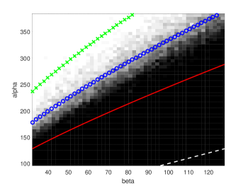
Figure 2: Result of simulation of the truncate-and-relax algorithm for $k=6$ and $n=500$. Each gray-scale block corresponds to a pair $(\alpha,\beta)$, and its color denotes the success rate over 30 trials (black corresponds to 0 success, and brighter color correspond to higher success rate). The solid line represents $I(\alpha,\beta)=1$, the circled line represents $I_{2}(\alpha,\beta)=1$, and the x-marked line represents $I_{sdp}(\alpha,\beta)=1$.

We ran a simulation to support our conjecture. For each $\alpha$ and $\beta$, we generated 30 random hypergraphs according to the model, and constructed the dual certificate for each hypergraph as in the proof of Theorem 2. When the constructed dual solution is positive-semidefinite, it was counted as a success. Figure 2 shows the result of the simulation and it suggests that the true phase transition occurs at $I_{2}(\alpha,\beta)=1$ as we proposed.

Appendix A Tail probability of weighted sum of binomial variables

In this section, we investigate the precise asymptotics of the tail probability of weighted sum of independent binomial variables. Using Theorem 10, we derive the formulas which were used to prove information-theoretic limits in section 3 and 4.

Theorem 10.

Let $r$ and $s$ be positive integers. Let $c_{1},c_{2},\cdots,c_{r}$ be non-zero real numbers. Let $h(n)$ be a non-decreasing function which is $\Omega(1)$ and $o(n^{s/2}/\log n)$. For each $i\in[r]$, let $Y_{i}$ be the random variable distributed as the binomial distribution $\mathrm{Bin}(N_{i},p_{i})$ where

$$N_{i}=(1+o_{n}(1))\rho_{i}\cdot h(n)\binom{n}{s}\quad\text{and}\quad p_{i}=(1+o_{n}(1))\alpha_{i}\cdot\frac{\log n}{\binom{n}{s}},$$

for some positive constant (not depending on $n$) $\rho_{i}$ and $\alpha_{i}$. Let $X=\sum_{i=1}^{r}c_{i}Y_{i}$. Suppose that (i) not all $c_{i}$ are positive, and (ii) $\sum_{i=1}^{r}c_{i}\alpha_{i}\rho_{i}>0$. Then, for any $\delta\in(-\infty,\sum_{i=1}^{r}c_{i}\alpha_{i}\rho_{i})$, we have

$$\operatorname*{\mathbb{P}}(X\leq(1+o_{n}(1))\delta\cdot h(n)\log n)=\exp\left(-(1+o_{n}(1))I^{*}\cdot h(n)\log n\right),$$

where

$$I^{*}=\max_{t\geq 0}\left(-t\delta+\sum_{i=1}^{r}\alpha_{i}\rho_{i}(1-e^{-tc_{i}})\right).$$

Proof.

Let us first prove the upper bound on the tail probability. Let $x=(1+o_{n}(1))\delta\cdot h(n)\log n$. Then, by Chebyshev-type inequality, for any $t\geq 0$ we have

$$\operatorname*{\mathbb{P}}(X\leq x) \leq \frac{\operatorname*{\mathbb{E}}e^{-tX}}{e^{-tx}}$$

$$= e^{tx}\prod_{i=1}^{r}\operatorname*{\mathbb{E}}e^{-tc_{i}Y_{i}}$$

$$= e^{tx}\prod_{i=1}^{r}\left(1-p_{i}(1-e^{-c_{i}t})\right)^{N_{i}}$$

$$\leq \exp\left(tx-\sum_{i=1}^{r}N_{i}p_{i}(1-e^{-c_{i}t})\right)$$

$$= \exp\left(-(1+o_{n}(1))h(n)\log n\cdot\left(-t\delta+\sum_{i=1}^{r}\alpha_{i}\rho_{i}(1-e^{-c_{i}t})\right)\right).$$

Here the fourth inequality follows from $1-x\leq e^{-x}$. By optimizing over $t\geq 0$, we get the desired bound.

To prove the lower bound, note that

$$\operatorname*{\mathbb{P}}(X\leq x)\geq\prod_{i=1}^{r}\operatorname*{\mathbb{P}}(Y_{i}=y_{i})=\prod_{i=1}^{r}\binom{N_{i}}{y_{i}}p_{i}^{y_{i}}(1-p_{i})^{N_{i}-y_{i}}$$

for any positive integers $y_{1},\cdots,y_{r}$ satisfying $\sum_{i=1}^{r}c_{i}y_{i}\leq x$.

Let $\phi(t)=-\delta t+\sum_{i=1}^{r}\alpha_{i}\rho_{i}(1-e^{-c_{i}t})$ and let $t^{*}$ be the maximizer of $\phi(t)$. Note that $\phi(t)$ is strictly convex, as

$$\phi^{\prime\prime}(t)=\sum_{i=1}^{r}c_{i}^{2}\alpha_{i}\rho_{i}e^{-c_{i}t}>0$$

for any $t\geq 0$. Moreover, $\phi^{\prime}(0)=\sum_{i=1}^{r}c_{i}\alpha_{i}\rho_{i}-\delta>0$ and $\lim_{t\to\infty}\phi^{\prime}(t)=-\infty$. Hence, there exists unique $t^{*}$ satisfying $\phi^{\prime}(t^{*})=0$, which is the maximizer of $\phi(t)$.

Let $\tau_{i}=\alpha_{i}\rho_{i}e^{-c_{i}t^{*}}$ for $i\in[r]$ and let $y_{1},\cdots,y_{r}$ be integers such that $\sum_{i=1}^{r}c_{i}y_{i}\leq x$ and $y_{i}=(1-o_{n}(1))\tau_{i}\cdot h(n)\log n$. Such $y_{i}$’s exist because

$$\sum_{i=1}^{r}c_{i}\tau_{i}=\sum_{i=1}^{r}c_{i}\alpha_{i}\rho_{i}e^{-c_{i}t^{*}}=\delta.$$

We are going to use the following bound for the binomial coefficient for $\ell\leq\sqrt{N}$

$$\binom{N}{\ell}\geq\frac{N^{\ell}}{4\cdot\ell!}.$$

By Stirling’s approximation, we have $\ell!\leq e\sqrt{\ell}\cdot\left(\frac{\ell}{e}\right)^{\ell}$ so

$$\log\binom{N}{\ell}\geq\ell\log\left(\frac{eN}{\ell}\right)-\log(4e\sqrt{\ell}).$$

Note that $y_{i}\ll\sqrt{N_{i}}$ since $h(n)=o(n^{s/2}/\log n)$. Hence,

$$\log\left(\binom{N_{i}}{y_{i}}p_{i}^{y_{i}}(1-p_{i})^{N_{i}-y_{i}}\right)\geq y_{i}\log\left(\frac{eN_{i}p_{i}}{(1-p_{i})y_{i}}\right)+N_{i}\log(1-p_{i})-\log(4e\sqrt{y_{i}}).$$

Moreover,

$$y_{i}\log\left(\frac{eN_{i}p_{i}}{(1-p_{i})y_{i}}\right) = (1-o_{n}(1))h(n)\log n\cdot\tau_{i}\log\left(\frac{e\alpha_{i}\rho_{i}}{\tau_{i}}\right)$$

$$N_{i}\log(1-p_{i}) = -(1+o_{n}(1))\alpha_{i}\rho_{i}\cdot h(n)\log n$$

$$\log(4e\sqrt{y_{i}}) = o(h(n)\log n).$$

We get

$$\operatorname*{\mathbb{P}}(X\leq x)\geq\exp\left(-(1+o_{n}(1))h(n)\log n\cdot\sum_{i=1}^{r}\left(\alpha_{i}\rho_{i}-\tau_{i}\log\left(\frac{e\alpha_{i}\rho_{i}}{\tau_{i}}\right)\right)\right).$$

Plugging in $\tau_{i}=\alpha_{i}\rho_{i}e^{-c_{i}t^{*}}$, we get

$$\sum_{i=1}^{r}\left(\alpha_{i}\rho_{i}-\tau_{i}\log\left(\frac{e\alpha_{i}\rho_{i}}{\tau_{i}}\right)\right) = \sum_{i=1}^{r}\left(\alpha_{i}\rho_{i}-\alpha_{i}\rho_{i}(1+c_{i}t^{*})e^{-c_{i}t^{*}}\right)$$

$$= -t^{*}\sum_{i=1}^{r}c_{i}\alpha_{i}\rho_{i}e^{-c_{i}t^{*}}+\sum_{i=1}^{r}\alpha_{i}\rho_{i}(1-e^{-c_{i}t^{*}})$$

$$= -\delta t^{*}+\sum_{i=1}^{r}\alpha_{i}\rho_{i}(1-e^{-c_{i}t^{*}})$$

$$= I^{*},$$

where the third equality follows from that $\sum_{i=1}^{r}c_{i}\alpha_{i}\rho_{i}e^{-c_{i}t^{*}}=\delta$. Hence,

$$\operatorname*{\mathbb{P}}(X\leq x)\geq\exp\left(-(1+o_{n}(1))I^{*}\cdot h(n)\log n\right)$$

as desired. ∎

We remark that the condition $h(n)=o(n^{s/2}/\log n)$ is not required for the upper bound.

A.1 Proof of Lemma 1

Let us restate the lemma for readers.

Lemma 4 (Lemma 1).

Let $X$ be a sum of independent Bernoulli variables such that $\operatorname*{\mathbb{E}}X=\Theta(\gamma\log n)$ where $\gamma=o_{n}(\log^{-1}n)$. Let $\delta$ be a positive number which decays to 0 as $n$ grows, with $\delta=\omega_{n}(\log^{-1}n)$. Then,

$$\operatorname*{\mathbb{P}}\left(X>\delta\log n\right)\leq n^{-\delta\log\frac{\delta}{\gamma}+o_{n}(1)}.$$

A standard Chernoff’s bound implies that

$$\operatorname*{\mathbb{P}}(X\geq t\operatorname*{\mathbb{E}}X)\leq\left(\frac{e^{t-1}}{t^{t}}\right)^{\operatorname*{\mathbb{E}}X}$$

for any $t\geq 0$. Let $t=\frac{\delta\log n}{\operatorname*{\mathbb{E}}X}$. Then,

$$\operatorname*{\mathbb{P}}(X\geq\delta\log n) \leq \exp\left((t-1-t\log t)\operatorname*{\mathbb{E}}X\right)$$

$$= \exp\left(\left(1-\log\frac{\delta\log n}{\operatorname*{\mathbb{E}}X}\right)\delta\log n-\operatorname*{\mathbb{E}}X\right)$$

$$= \exp\left(\left(1-\log\frac{\delta}{\gamma}+O(1)\right)\delta\log n-o_{n}(1)\right)$$

$$= n^{-\delta\log\frac{\delta}{\gamma}+o_{n}(1)}$$

as desired.

A.2 Proof of Lemma 2

Let $a\in U_{A}$. Recall that

$$X_{a}=\sum_{e:e\cap U=\{a\}}c_{e}(A_{\mathcal{H}})_{e},$$

where $c_{e}=\Sigma_{e}-\Sigma^{(ab)}_{e}$ for any $b\in U_{B}$. Concretely, the value of $c_{e}$ for $e$ satisfying $e\cap U=\{a\}$ is determined by the size of intersection of $e\setminus\{a\}$ and $A\setminus U_{A}$ as follows:

$$c_{e}=\begin{cases}+1&\text{if $e\setminus\{a\}\subseteq A\setminus U_{A}$}\\ -1&\text{if $(e\setminus\{a\})\cap(A\setminus U_{A})=\emptyset$}\\ 0&\text{otherwise}.\end{cases}$$

Hence, $X_{a}=Y_{1}-Y_{2}$ where $Y_{1}$ and $Y_{2}$ are independent random variables such that $Y_{1}\sim\mathrm{Bin}(N_{1},p)$ and $Y_{2}\sim\mathrm{Bin}(N_{2},q)$ with

$$N_{1}=\binom{n/2-|U_{A}|}{k-1}\quad\text{and}\quad N_{2}=\binom{n/2-|U_{B}|}{k-1}.$$

Using Theorem 10 with $c_{1}=1$, $c_{2}=-1$, $\alpha_{1}=\alpha$, $\alpha_{2}=\beta$, $\rho_{1}=\rho_{2}=\frac{1}{2^{k-1}}$, $h(n)=1$ and $\delta=0$, we get

$$\operatorname*{\mathbb{P}}\left(X_{a}\leq\frac{\log n}{\log\log n}\right)=\exp\left(-(1+o_{n}(1))I^{*}\cdot\log n\right),$$

where

$$I^{*} = \max_{t\geq 0}\sum_{i=1}^{2}\alpha_{i}\rho_{i}(1-e^{-c_{i}t})$$

$$= \max_{t\geq 0}\frac{1}{2^{k-1}}\left(\alpha(1-e^{-t})+\beta(1-e^{t})\right).$$

The maximum is attained at $t^{*}=\frac{1}{2}\log\left(\frac{\alpha}{\beta}\right)>0$ and

$$I^{*}=\frac{1}{2^{k-1}}\left(\sqrt{\alpha}-\sqrt{\beta}\right)^{2}=1-\epsilon.$$

Hence,

$$\operatorname*{\mathbb{P}}\left(X_{a}\leq\frac{\log n}{\log\log n}\right)\geq n^{-1+\epsilon-o_{n}(1)}$$

as desired.

A.3 Proof of the tail bound in Theorem 8

We recall that $X_{a}$ is defined as

$$X_{a}=\sum_{e:e\cap U=\{a\}}(A_{\mathcal{H}})_{a}\left(\sum_{ij\subseteq e}\sigma_{i}\sigma_{j}-\sigma^{(a)}_{i}\sigma^{(a)}_{j}\right).$$

By definition of $\sigma^{(a)}$, we have

$$\left(\sum_{ij\subseteq e}\sigma_{i}\sigma_{j}-\sigma^{(a)}_{i}\sigma^{(a)}_{j}\right) = 2\sigma_{a}\sum_{i\in e\setminus\{a\}}\sigma_{i}$$

$$= 2\left(k-1-2|e\cap B|\right).$$

Hence, $X_{a}=\sum_{r=0}^{k-1}c_{r}Y_{r}$ where $c_{r}=2(k-1-2r)$ and $Y_{r}\sim\mathrm{Bin}(N_{r},p_{r})$ with

$$N_{r}=\binom{n/2-|U_{A}|}{k-1-r}\binom{n/2-|U_{B}|}{r}=(1+o_{n}(1))\frac{1}{2^{k-1}}\binom{k-1}{r}\binom{n}{k-1}$$

and

$$p_{r}=\begin{cases}p&\text{if $r=0$}\\ q&\text{otherwise.}\end{cases}$$

Using Theorem 10 with

$$c_{r}=2(k-1-2r),\quad\rho_{r}=\frac{1}{2^{k-1}}\binom{k-1}{r},\quad\alpha_{r}=\begin{cases}\alpha&\text{if $r=0$}\\ \beta&\text{otherwise,}\end{cases}$$

and $h(n)=1$ and $\delta=0$, we have

$$\operatorname*{\mathbb{P}}\left(X_{a}\leq-\frac{2\log n}{\log\log n}\right)=\exp\left(-(1+o_{n}(1))I_{2}\cdot\log n\right)$$

where

$$I_{2} = \max_{t\geq 0}\sum_{r=0}^{k-1}\alpha_{i}\rho_{i}(1-e^{-c_{i}t})$$

$$= \max_{t\geq 0}\frac{1}{2^{k-1}}\left(\alpha(1-e^{-(k-1)t})+\beta\sum_{r=1}^{k-1}\binom{k-1}{r}(1-e^{-(k-1-2r)t})\right),$$

as desired.

Appendix B Miscellaneous proofs

B.1 Proof of Proposition 1

Recall that the MLE $\widehat{\sigma}_{MLE}(H)$ is defined as

$$\widehat{\sigma}_{MLE}(H)=\operatorname*{\mathrm{argmax}}_{x\in\{\pm 1\}^{V}:\mathbf{1}^{T}x=0}f_{H}(x),$$

where $f_{H}(x)=\log\operatorname*{\mathbb{P}}_{(\sigma,\mathcal{H})}(\mathcal{H}=H|\sigma=x)$. Note that

$$f_{H}(x) = \log\operatorname*{\mathbb{P}}(\mathcal{H}=H|\sigma=x)$$

$$= \log\left(\prod_{e\in\binom{V}{k}}\operatorname*{\mathbb{P}}(e\in E(\mathcal{H})|\sigma=x)^{(A_{H})_{e}}\operatorname*{\mathbb{P}}(e\not\in E(\mathcal{H})|\sigma=x)^{1-(A_{H})_{e}}\right)$$

$$= \sum_{\begin{subarray}{c}e\in\binom{V}{k}\\ e\text{: in-cl. w.r.t. $x$}\end{subarray}}(A_{H})_{e}\log p+(1-(A_{H})_{e})\log(1-p)$$

$$+\sum_{\begin{subarray}{c}e\in\binom{V}{k}\\ e\text{: cr.-cl. w.r.t. $x$}\end{subarray}}(A_{H})_{e}\log q+(1-(A_{H})_{e})\log(1-q)$$

$$= C+\log\left(\frac{p}{1-p}\right)\langle A_{H},x^{\mathchoice{\mathbin{\ooalign{$\displaystyle=$\crcr$\displaystyle\ovoid$}}}{\mathbin{\ooalign{$\textstyle=$\crcr$\textstyle\ovoid$}}}{\mathbin{\ooalign{$\scriptstyle=$\crcr$\scriptstyle\ovoid$}}}{\mathbin{\ooalign{$\scriptscriptstyle=$\crcr$\scriptscriptstyle\ovoid$}}}k}\rangle+\log\left(\frac{q}{1-q}\right)\langle A_{H},1-x^{\mathchoice{\mathbin{\ooalign{$\displaystyle=$\crcr$\displaystyle\ovoid$}}}{\mathbin{\ooalign{$\textstyle=$\crcr$\textstyle\ovoid$}}}{\mathbin{\ooalign{$\scriptstyle=$\crcr$\scriptstyle\ovoid$}}}{\mathbin{\ooalign{$\scriptscriptstyle=$\crcr$\scriptscriptstyle\ovoid$}}}k}\rangle,$$

with

$$C = \log(1-p)\cdot\#(e:\text{ in-cl. w.r.t. $x$})+\log(1-q)\cdot\#(e:\text{ cr.-cl. w.r.t. $x$})$$

$$= 2\binom{n/2}{k}\log(1-p)+\left(\binom{n}{k}-2\binom{n/2}{k}\right)\log(1-q).$$

We note that $C$ is a constant not depending on $x$. Also, $\langle A_{H},1\rangle$ is independent of $x$. We get

$$\widehat{\sigma}_{MLE}(H)=\operatorname*{\mathrm{argmax}}_{x\in\{\pm 1\}^{V}:\mathbf{1}^{T}x=0}\log\left(\frac{p(1-q)}{q(1-p)}\right)\langle A_{H},x^{\mathchoice{\mathbin{\ooalign{$\displaystyle=$\crcr$\displaystyle\ovoid$}}}{\mathbin{\ooalign{$\textstyle=$\crcr$\textstyle\ovoid$}}}{\mathbin{\ooalign{$\scriptstyle=$\crcr$\scriptstyle\ovoid$}}}{\mathbin{\ooalign{$\scriptscriptstyle=$\crcr$\scriptscriptstyle\ovoid$}}}k}\rangle.$$

It implies that

$$\widehat{\sigma}_{MLE}(H)=\begin{cases}\displaystyle\operatorname*{\mathrm{argmax}}_{x\in\{\pm 1\}^{V}:\mathbf{1}^{T}x=0}\langle A_{H},x^{\mathchoice{\mathbin{\ooalign{$\displaystyle=$\crcr$\displaystyle\ovoid$}}}{\mathbin{\ooalign{$\textstyle=$\crcr$\textstyle\ovoid$}}}{\mathbin{\ooalign{$\scriptstyle=$\crcr$\scriptstyle\ovoid$}}}{\mathbin{\ooalign{$\scriptscriptstyle=$\crcr$\scriptscriptstyle\ovoid$}}}k}\rangle&\text{if $p>q$}\\ \displaystyle\operatorname*{\mathrm{argmin}}_{x\in\{\pm 1\}^{V}:\mathbf{1}^{T}x=0}\langle A_{H},x^{\mathchoice{\mathbin{\ooalign{$\displaystyle=$\crcr$\displaystyle\ovoid$}}}{\mathbin{\ooalign{$\textstyle=$\crcr$\textstyle\ovoid$}}}{\mathbin{\ooalign{$\scriptstyle=$\crcr$\scriptstyle\ovoid$}}}{\mathbin{\ooalign{$\scriptscriptstyle=$\crcr$\scriptscriptstyle\ovoid$}}}k}\rangle&\text{if $p<q$}\end{cases}$$

since $\log\left(\frac{p(1-q)}{q(1-p)}\right)$ is positive if $p>q$ and it is negative if $p<q$.

B.2 Proof of Lemma 3

We recall that

$$Y_{e}=\left((\mathbf{1}_{e}^{T}\sigma_{e})\mathrm{diag}(\sigma_{e})-\sigma_{e}\sigma_{e}^{T}\right)\Pi\left((\mathbf{1}_{e}^{T}\sigma_{e})\mathrm{diag}(\sigma_{e})-\sigma_{e}\sigma_{e}^{T}\right),$$

where $\Pi=I-\frac{1}{n}\sigma\sigma^{T}-\frac{1}{n}{\mathbf{1}\mathbf{1}^{T}}$. We defined $\Sigma$ as

$$\Sigma=\sum_{e}\operatorname*{\mathbb{E}}(A_{\mathcal{H}})_{e}\cdot Y_{e}=p\sum_{e:e\text{ is in-cl.}}Y_{e}+q\sum_{e:e\text{ is cross-cl.}}Y_{e}.$$

Lemma 5 (Lemma 3).

$\Sigma=c_{1}\cdot\frac{1}{n}\sigma\sigma^{T}+c_{2}\cdot\Pi$ where

$$c_{1}=(k-1)\beta\log n+O\left(\frac{\log n}{n}\right)$$

and

$$c_{2}=2(k-1)\left(\frac{k}{2^{k}}\alpha+\left(1-\frac{k}{2^{k}}\right)\beta\right)\log n+O\left(\frac{\log n}{n}\right).$$

We note that $\sum_{e:e\text{ is in-cl.}}Y_{e}$ and $\sum_{e:e\text{ is cross-cl.}}Y_{e}$ are invariant under any permutation on $V$ preserving $\sigma$. It implies that the both matrices and $\Sigma$ are in the span of $\Pi$, $\sigma\sigma^{T}$ and $\mathbf{1}\mathbf{1}^{T}$. Moreover,

$$\left((\mathbf{1}_{e}^{T}\sigma_{e})\mathrm{diag}(\sigma_{e})-\sigma_{e}\sigma_{e}^{T}\right)\mathbf{1}=(\mathbf{1}_{e}^{T}\sigma_{e})\sigma_{e}-(\mathbf{1}^{T}\sigma_{e})\sigma_{e}=0$$

so $\langle Y_{e},\mathbf{1}\mathbf{1}^{T}\rangle=0$. Hence,

$$\Sigma=\frac{\langle\Sigma,\Pi\rangle}{\langle\Pi,\Pi\rangle}\Pi+\langle\Sigma,\frac{1}{n}\sigma\sigma^{T}\rangle\cdot\frac{1}{n}\sigma\sigma^{T}.$$

It implies that

$$c_{1} = \langle\Sigma,\frac{1}{n}\sigma\sigma^{T}\rangle=\frac{1}{n}\sigma^{T}\Sigma\sigma$$

$$c_{2} = \frac{\langle\Sigma,\Pi\rangle}{\langle\Pi,\Pi\rangle}=\frac{1}{n-2}\left(tr(\Sigma)-\frac{1}{n}\sigma^{T}\Sigma\sigma\right)$$

Now, let us first compute $\sigma^{T}\Sigma\sigma$. For simplicity, let $r=\frac{1}{2}(k-\mathbf{1}_{e}^{T}\sigma_{e})$. Then,

$$\sigma^{T}Y_{e}\sigma = \sigma^{T}\left((k-2r)\mathrm{diag}(\sigma_{e})-\sigma_{e}\sigma_{e}^{T}\right)\Pi\left((k-2r)\mathrm{diag}(\sigma_{e})-\sigma_{e}\sigma_{e}^{T}\right)\sigma$$

$$= \left((k-2r)\mathbf{1}_{e}-k\sigma_{e}\right)^{T}\Pi\left((k-2r)\mathbf{1}_{e}-k\sigma_{e}\right)$$

$$= \|(k-2r)\mathbf{1}_{e}-k\sigma_{e}\|_{2}^{2}-\frac{1}{n}((k-2r)\mathbf{1}_{e}-k\sigma_{e})^{T}\sigma)^{2}$$

$$= (k^{3}-k(k-2r)^{2})-\frac{1}{n}\left((k-2r)^{2}-k^{2}\right)^{2}$$

$$= 4kr(k-r)-\frac{16}{n}r^{2}(k-r)^{2}.$$

In particular, $\sigma^{T}Y_{e}\sigma=0$ if $e$ is in-cluster with respect to $\sigma$. Hence,

$$\sigma^{T}\Sigma\sigma = q\sum_{e:e\text{ is cross-cl.}}\sigma^{T}Y_{e}\sigma$$

$$= q\sum_{r=1}^{k-1}\left(4kr(k-r)-\frac{16}{n}r^{2}(k-r)^{2}\right)\binom{n/2}{r}\binom{n/2}{k-r}.$$

We note that for any $s,t\in\{1,2\}$, we have

$$\sum_{r=1}^{k-1}\binom{r}{s}\binom{k-r}{t}\binom{n/2}{r}\binom{n/2}{k-r} = \binom{n/2}{s}\binom{n/2}{t}\binom{n-s-t}{k-s-t}$$

$$= \binom{n/2}{s}\binom{n/2}{t}\binom{n}{k}\binom{k}{s+t}\binom{n}{s+t}^{-1}.$$

Hence,

$$\sum_{r=1}^{k-1}r(k-r)\binom{n/2}{r}\binom{n/2}{k-r} = \binom{n}{k}\frac{\binom{k}{2}\binom{n/2}{1}^{2}}{\binom{n}{2}}$$

$$= \binom{n}{k}\frac{k(k-1)n^{2}}{4n(n-1)}=\frac{k(k-1)}{4}\binom{n}{k}+O(n^{k-1}).$$

and

$$\frac{1}{n}\sum_{r=1}^{k-1}r^{2}(k-r)^{2}\binom{n/2}{r}\binom{n/2}{k-r}=O(n^{k-1}).$$

Hence,

$$c_{1}=\frac{1}{n}\sigma^{T}\Sigma\sigma=(k-1)\beta\log n+O\left(\frac{\log n}{n}\right).$$

On the other hand,

$$tr(Y_{e}) = tr\left(\left((k-2r)\mathrm{diag}(\sigma_{e})-\sigma_{e}\sigma_{e}^{T}\right)^{2}\Pi\right)$$

$$= tr\left(\left((k-2r)\mathrm{diag}(\sigma_{e})-\sigma_{e}\sigma_{e}^{T}\right)^{2}\right)-\frac{1}{n}\left\|\left((k-2r)\mathrm{diag}(\sigma_{e})-\sigma_{e}\sigma_{e}^{T}\right)\sigma\right\|_{2}^{2}$$

$$= \left((k-2)(k-2r)^{2}+k^{2}\right)-\frac{1}{n}\|(k-2r)\mathbf{1}_{e}-k\sigma_{e}\|_{2}^{2}$$

$$= \left((k-2)(k-2r)^{2}+k^{2}\right)-\frac{1}{n}(k^{3}-k(k-2r)^{2})$$

$$= (k^{3}-k^{2})-4(k-2+\frac{k}{n})r(k-r),$$

so we have

$$tr(\Sigma) = (k^{3}-k^{2})\left(q\binom{n}{k}+2(p-q)\binom{n/2}{k}\right)-4q\left(k-2+\frac{k}{n}\right)\cdot\frac{n^{2}}{4}\binom{n-2}{k-2}$$

$$= \left[(k^{2}-k)\left(\beta+\frac{\alpha-\beta}{2^{k-1}}\right)-(k-1)(k-2)\beta\right]n\log n+O(\log n).$$

and hence

$$c_{2} = \frac{1}{n-2}\left(tr(\Sigma)-\frac{1}{n}\sigma^{T}\Sigma\sigma\right)$$

$$= 2(k-1)\left(\frac{k}{2^{k}}\alpha+\left(1-\frac{k}{2^{k}}\right)\beta\right)\log n+O\left(\frac{\log n}{n}\right).$$

References

• [ABB06] Sameer Agarwal, Kristin Branson, and Serge Belongie. Higher order learning with graphs. In Proceedings of the 23rd international conference on Machine learning, pages 17–24. ACM, 2006.
• [Abb18] Emmanuel Abbe. Community detection and stochastic block models: Recent developments. Journal of Machine Learning Research, 18(177):1–86, 2018.
• [ABH16] Emmanuel Abbe, Afonso S Bandeira, and Georgina Hall. Exact recovery in the stochastic block model. IEEE Transactions on Information Theory, 62(1):471–487, 2016.
• [ACKZ15] Maria Chiara Angelini, Francesco Caltagirone, Florent Krzakala, and Lenka Zdeborová. Spectral detection on sparse hypergraphs. In Communication, Control, and Computing (Allerton), 2015 53rd Annual Allerton Conference on, pages 66–73. IEEE, 2015.
• [ALS16] Kwangjun Ahn, Kangwook Lee, and Changho Suh. Community recovery in hypergraphs. In Communication, Control, and Computing (Allerton), 2016 54th Annual Allerton Conference on, pages 657–663. IEEE, 2016.
• [ALS18] Kwangjun Ahn, Kangwook Lee, and Changho Suh. Hypergraph spectral clustering in the weighted stochastic block model. arXiv preprint arXiv:1805.08956, 2018.
• [ALZM+05] Sameer Agarwal, Jongwoo Lim, Lihi Zelnik-Manor, Pietro Perona, David Kriegman, and Serge Belongie. Beyond pairwise clustering. In Computer Vision and Pattern Recognition, 2005. CVPR 2005. IEEE Computer Society Conference on, volume 2, pages 838–845. IEEE, 2005.
• [AS15a] Emmanuel Abbe and Colin Sandon. Community detection in general stochastic block models: Fundamental limits and efficient algorithms for recovery. In Foundations of Computer Science (FOCS), 2015 IEEE 56th Annual Symposium on, pages 670–688. IEEE, 2015.
• [AS15b] Emmanuel Abbe and Colin Sandon. Detection in the stochastic block model with multiple clusters: proof of the achievability conjectures, acyclic bp, and the information-computation gap. arXiv preprint arXiv:1512.09080, 2015.
• [AS15c] Emmanuel Abbe and Colin Sandon. Recovering communities in the general stochastic block model without knowing the parameters. In Advances in neural information processing systems, pages 676–684, 2015.
• [AS16] Emmanuel Abbe and Colin Sandon. Achieving the ks threshold in the general stochastic block model with linearized acyclic belief propagation. In Advances in Neural Information Processing Systems, pages 1334–1342, 2016.
• [Ban16] Afonso S Bandeira. Random Laplacian Matrices and Convex Relaxations, 2016.
• [BCOK10] Michael Behrisch, Amin Coja-Oghlan, and Mihyun Kang. The order of the giant component of random hypergraphs. Random Structures & Algorithms, 36(2):149–184, 2010.
• [Bol98] Béla Bollobás. Random graphs. In Modern graph theory, pages 215–252. Springer, 1998.
• [BvH16] Afonso S Bandeira and Ramon van Handel. Sharp nonasymptotic bounds on the norm of random matrices with independent entries. Annals of Probability, 44(4):2479–2506, 2016.
• [CAT16] Irineo Cabreros, Emmanuel Abbe, and Aristotelis Tsirigos. Detecting community structures in hi-c genomic data. In Information Science and Systems (CISS), 2016 Annual Conference on, pages 584–589. IEEE, 2016.
• [CKK15] Oliver Cooley, Mihyun Kang, and Christoph Koch. Evolution of high-order connected components in random hypergraphs. Electronic Notes in Discrete Mathematics, 49:569–575, 2015.
• [CLR16] T Tony Cai, Tengyuan Liang, and Alexander Rakhlin. Inference via message passing on partially labeled stochastic block models. arXiv preprint arXiv:1603.06923, 2016.
• [CLW+18] I Chien, Chung-Yi Lin, I Wang, et al. On the minimax misclassification ratio of hypergraph community detection. arXiv preprint arXiv:1802.00926, 2018.
• [COMS07] Amin Coja-Oghlan, Cristopher Moore, and Vishal Sanwalani. Counting connected graphs and hypergraphs via the probabilistic method. Random Structures & Algorithms, 31(3):288–329, 2007.
• [CX16] Yudong Chen and Jiaming Xu. Statistical-computational tradeoffs in planted problems and submatrix localization with a growing number of clusters and submatrices. Journal of Machine Learning Research, 17(27):1–57, 2016.
• [CY06] Jingchun Chen and Bo Yuan. Detecting functional modules in the yeast protein–protein interaction network. Bioinformatics, 22(18):2283–2290, 2006.
• [DAM16] Yash Deshpande, Emmanuel Abbe, and Andrea Montanari. Asymptotic mutual information for the binary stochastic block model. In Information Theory (ISIT), 2016 IEEE International Symposium on, pages 185–189. IEEE, 2016.
• [DKMZ11] Aurelien Decelle, Florent Krzakala, Cristopher Moore, and Lenka Zdeborová. Asymptotic analysis of the stochastic block model for modular networks and its algorithmic applications. Physical Review E, 84(6):066106, 2011.
• [FO05] Uriel Feige and Eran Ofek. Spectral techniques applied to sparse random graphs. Random Structures & Algorithms, 27(2):251–275, 2005.
• [GD14] Debarghya Ghoshdastidar and Ambedkar Dukkipati. Consistency of spectral partitioning of uniform hypergraphs under planted partition model. In Advances in Neural Information Processing Systems, pages 397–405, 2014.
• [GD15a] Debarghya Ghoshdastidar and Ambedkar Dukkipati. A provable generalized tensor spectral method for uniform hypergraph partitioning. In International Conference on Machine Learning, pages 400–409, 2015.
• [GD15b] Debarghya Ghoshdastidar and Ambedkar Dukkipati. Spectral clustering using multilinear svd: Analysis, approximations and applications. In AAAI, pages 2610–2616, 2015.
• [GD+17] Debarghya Ghoshdastidar, Ambedkar Dukkipati, et al. Consistency of spectral hypergraph partitioning under planted partition model. The Annals of Statistics, 45(1):289–315, 2017.
• [Gov05] Venu Madhav Govindu. A tensor decomposition for geometric grouping and segmentation. In Computer Vision and Pattern Recognition, 2005. CVPR 2005. IEEE Computer Society Conference on, volume 1, pages 1150–1157. IEEE, 2005.
• [GW95] Michel X Goemans and David P Williamson. Improved approximation algorithms for maximum cut and satisfiability problems using semidefinite programming. Journal of the ACM (JACM), 42(6):1115–1145, 1995.
• [GZCN09] Gourab Ghoshal, Vinko Zlatić, Guido Caldarelli, and MEJ Newman. Random hypergraphs and their applications. Physical Review E, 79(6):066118, 2009.
• [HWX16] Bruce Hajek, Yihong Wu, and Jiaming Xu. Achieving exact cluster recovery threshold via semidefinite programming. IEEE Transactions on Information Theory, 62(5):2788–2797, 2016.
• [JMRT16] Adel Javanmard, Andrea Montanari, and Federico Ricci-Tersenghi. Phase transitions in semidefinite relaxations. Proceedings of the National Academy of Sciences, 113(16):E2218–E2223, 2016.
• [KBG17] Chiheon Kim, Afonso S Bandeira, and Michel X Goemans. Community detection in hypergraphs, spiked tensor models, and sum-of-squares. In Sampling Theory and Applications (SampTA), 2017 International Conference on, pages 124–128. IEEE, 2017.
• [LCW17] Chung-Yi Lin, I Eli Chien, and I-Hsiang Wang. On the fundamental statistical limit of community detection in random hypergraphs. In Information Theory (ISIT), 2017 IEEE International Symposium on, pages 2178–2182. IEEE, 2017.
• [LKZ17] Thibault Lesieur, Florent Krzakala, and Lenka Zdeborová. Constrained low-rank matrix estimation: Phase transitions, approximate message passing and applications. Journal of Statistical Mechanics: Theory and Experiment, 2017(7):073403, 2017.
• [LML+17] Thibault Lesieur, Léo Miolane, Marc Lelarge, Florent Krzakala, and Lenka Zdeborová. Statistical and computational phase transitions in spiked tensor estimation. arXiv preprint arXiv:1701.08010, 2017.
• [LSY03] Greg Linden, Brent Smith, and Jeremy York. Amazon. com recommendations: Item-to-item collaborative filtering. IEEE Internet computing, 7(1):76–80, 2003.
• [Mas14] Laurent Massoulié. Community detection thresholds and the weak ramanujan property. In Proceedings of the 46th Annual ACM Symposium on Theory of Computing, pages 694–703. ACM, 2014.
• [MN12] Tom Michoel and Bruno Nachtergaele. Alignment and integration of complex networks by hypergraph-based spectral clustering. Physical Review E, 86(5):056111, 2012.
• [MNS12] Elchanan Mossel, Joe Neeman, and Allan Sly. Stochastic block models and reconstruction. arXiv preprint arXiv:1202.1499, 2012.
• [MNS13] Elchanan Mossel, Joe Neeman, and Allan Sly. A proof of the block model threshold conjecture. arXiv preprint arXiv:1311.4115, 2013.
• [MPN+99] Edward M Marcotte, Matteo Pellegrini, Ho-Leung Ng, Danny W Rice, Todd O Yeates, and David Eisenberg. Detecting protein function and protein-protein interactions from genome sequences. Science, 285(5428):751–753, 1999.
• [NWS02] Mark EJ Newman, Duncan J Watts, and Steven H Strogatz. Random graph models of social networks. Proceedings of the National Academy of Sciences, 99(suppl 1):2566–2572, 2002.
• [SC11] Shaghayegh Sahebi and William W Cohen. Community-based recommendations: a solution to the cold start problem. In Workshop on recommender systems and the social web, RSWEB, 2011.
• [SM00] Jianbo Shi and Jitendra Malik. Normalized cuts and image segmentation. IEEE Transactions on pattern analysis and machine intelligence, 22(8):888–905, 2000.
• [Tro12] Joel A Tropp. User-friendly tail bounds for sums of random matrices. Foundations of computational mathematics, 12(4):389–434, 2012.
• [VSMGA14] Greg Ver Steeg, Cristopher Moore, Aram Galstyan, and Armen Allahverdyan. Phase transitions in community detection: A solvable toy model. EPL (Europhysics Letters), 106(4):48004, 2014.
• [Vu14] Van A N Vu. A simple SVD algorithm for finding hidden partitions. pages 1–12, 2014.
• [ZGC09] Vinko Zlatić, Gourab Ghoshal, and Guido Caldarelli. Hypergraph topological quantities for tagged social networks. Physical Review E, 80(3):036118, 2009.