High-order, Dispersionless “Fast-Hybrid” Wave Equation Solver. Part I: $\mathcal{O}(1)$ Sampling Cost via Incident-Field Windowing and Recentering

Abstract

This paper proposes a frequency/time hybrid integral-equation method for the time dependent wave equation in two and three-dimensional spatial domains. Relying on Fourier Transformation in time, the method utilizes a fixed (time-independent) number of frequency-domain integral-equation solutions to evaluate, with superalgebraically-small errors, time domain solutions for arbitrarily long times. The approach relies on two main elements, namely, 1) A smooth time-windowing methodology that enables accurate band-limited representations for arbitrarily-long time signals, and 2) A novel Fourier transform approach which, in a time-parallel manner and without causing spurious periodicity effects, delivers numerically dispersionless spectrally-accurate solutions. A similar hybrid technique can be obtained on the basis of Laplace transforms instead of Fourier transforms, but we do not consider the Laplace-based method in the present contribution. The algorithm can handle dispersive media, it can tackle complex physical structures, it enables parallelization in time in a straightforward manner, and it allows for time leaping—that is, solution sampling at any given time $T$ at $\mathcal{O}(1)$-bounded sampling cost, for arbitrarily large values of $T$, and without requirement of evaluation of the solution at intermediate times. The proposed frequency-time hybridization strategy, which generalizes to any linear partial differential equation in the time domain for which frequency-domain solutions can be obtained (including e.g. the time-domain Maxwell equations), and which is applicable in a wide range of scientific and engineering contexts, provides significant advantages over other available alternatives such as volumetric discretization, time-domain integral equations, and convolution-quadrature approaches.

65M80, 65T99, 65R20

1 Introduction

This paper, Part I of a two-part contribution, proposes a fast frequency-time hybrid integral-equation method for the solution of the time domain wave equation in two- and three-dimensional spatial domains. Relying on 1) A smooth time-windowing methodology that enables accurate band-limited representations for arbitrary long time signals, and 2) A novel FFT-accelerated Fourier transform strategy (which, without requiring finer and finer meshes as time grows, is amenable to time parallelism and does not give rise to spurious periodicity effects), the proposed approach delivers numerically dispersionless solutions with numerical errors that decay faster than any power of the frequency mesh-size used. For definiteness, the theoretical discussions in the present paper are restricted to configurations for which the time-dependent excitations propagate along a single incidence direction—which is, in fact, one of the most common incident field arising in applications—but our numerical-results section includes examples that incorporate incident fields of other (generic) types (Table 4 and Figure 7). The development of algorithms for treatment of the general-incidence case on the basis of precomputation strategies that utilize plane waves or other bases of incident fields will be left for future work (but see Remark 1). Similarly, general window tracking strategies based on characteristics of field-decay in two and three-dimensional configurations (including treatment of trapping structures), and parallel implementations exploiting the methodology’s inherent parallelism in space and time, will be presented elsewhere.

In practice the proposed methodology enjoys a number of attractive properties, including high accuracy without numerical dispersion error; an ability to effectively leverage existing frequency-domain scattering solvers for arbitrary, potentially complex spatial domains; an ability to treat dispersive media; dimensional reduction (if integral equation methods are used as the frequency domain solver components); natural parallel decoupling of the associated frequency-domain components; and, most notably, time-leaping, time parallelism, and $\mathcal{O}(1)$ cost for solution sampling at arbitrarily-large times without requirement of intermediate time evaluation. A similar hybrid technique can be obtained on the basis of Laplace transforms instead of Fourier transforms. Use of the Laplace-based technique would be advantageous for treatment of certain types of initial/boundary-value problems with non-vanishing initial conditions, but we do not consider a Laplace-based approach in any detail in the present contribution. We also note that the ideas inherent in the proposed fast-hybrid approach may be applied, more generally, to any time-domain problem whose frequency-domain counterpart can be treated by means of an efficient frequency-domain approach.

A wide literature exists, of course, for the treatment of the classical wave equation problem. Among the many approaches utilized in this context we find finite-difference and finite-element time domain methods [55, 43] (FDTD and FETD, respectively), retarded potential boundary integral equation methods [6, 38, 58, 33], Huygens-preserving treatments for odd-dimensional spatial domains [52], and, most closely related to the present work, two hybrid frequency-time methodologies, namely, the Laplace-transform/finite-difference convolution quadrature method [45, 10, 7, 9, 11, 8, 15], and the Fourier-transform/operator-expansion method [47]. A brief discussion of the character of these methodologies is presented in what follows.

The FDTD approach and related finite-difference methods underlie most of the wave-equation solvers used in practice. In these approaches the solution on the entire spatial domain is obtained via finite difference discretization of the PDE in both space and time. For the ubiquitous exterior-domain problems, the use of absorbing boundary conditions is necessary to render the problem computationally feasible—which has in fact been an important and challenging problem in itself [39, 14, 32, 13]. Most importantly, however, finite-difference methods suffer from numerical dispersion, and they therefore require the use of fine spatial meshes (and, thus, fine temporal meshes, for stability) to produce accurate solutions. Numerical dispersion errors therefore present a significant obstacle for high frequency and/or long time simulations via methods based on finite-difference spatial discretizations. FETD methods provide an additional element of geometric generality, but they require creation of high-quality finite element meshes (which can be challenging for complex three-dimensional structures). Further, like FDTD methods, they entail use of absorbing boundary conditions, and they also generally give rise to detrimental dispersion errors (also called “pollution errors” in this context [3]).

Integral-equation formulations based on direct discretization of the time-domain retarded-potential Green’s function, on the other hand, require treatment of the Dirac delta function and thus give rise to integration domains given by the intersection of the light cone with the overall scattering surface [6, 38]. These approaches generally result in relatively complex overall schemes for which it has proven rather challenging to ensure stability [33], and which have typically been implemented in low-order accuracy setups and, thus, with significant numerical dispersion error. Accelerated versions of these methods have also been proposed [58]. Motivated by the work in [33], temporally and spatially high-order time domain integral equation schemes have recently been proposed [12]. Loosely related to this class of methods are recent work on discretizations which are Huygens-preserving—that is, treatments of the retarded potential operators with the advantage that they do not entail an increasing amount of computational work for increasing time, at least in odd dimensions [52].

Hybrid time-frequency methods rely on transform techniques to evaluate time domain solutions by synthesis from sets of frequency domain solutions; clearly the necessary solutions of (decoupled) frequency-domain problems can be obtained via parallel computation. The Convolution Quadrature (CQ) method [45] is a prominent example of this class of approaches. This method relies on the combination of a finite-difference time discretization and a Laplace transformation to effectively reduce the time domain wave equation to a set of modified Helmholtz equations over a range of frequencies. There has additionally been some interest in the direct use of Fourier transformations in time [47, 30] to decouple the time-domain problem into frequency-domain sub-problems. In detail, assuming a Gaussian-modulated incident time-pulse, the approach [47] evaluates Fourier integrals on the basis of a Gauss-Hermite quadrature rule, and it obtains the necessary frequency-domain solutions by means of a certain “operator expansion method”; earlier efforts in a single spatial dimension [30] recognized the advantages of hybrid methods for simulating wave phenomena in complex, and specifically attenuating media, but relied on a low-order accurate midpoint quadrature rule for Fourier integrals. In all cases, however, the number of frequency-domain solutions required, and hence the associated computing and memory costs, grow linearly with the number $N$ of time steps used to evolve the solution to a given final time $T$. (A more detailed discussion of previous hybrid methods, including CQ and direct-transform methods, is presented in Section 2.2.)

To address these difficulties, for incident pulses of arbitrary duration the proposed approach employs a smoothly time-windowed Fourier transformation technique (detailed in Section 3), which, without resorting to use of refined frequency discretizations, re-centers the solution in time and thus effectively handles the fast oscillations that occur in the scattering solution as a function of the Fourier-transform variable $\omega$. Therefore, in contrast to the CQ and the direct-transform methods, the new approach can be applied in the presence of arbitrary incident fields on the basis of a fixed set of frequency-domain solutions. Other favorable properties of the method include its time-parallel character, its time-leaping abilities and $\mathcal{O}(1)$ cost of evaluation at any given time, however large, and, therefore, its $\mathcal{O}(N)$ cost for a total full $N$ timestep history of the solution. The algorithm remains uniformly (spectrally) accurate in time for arbitrarily long times, with complete absence of temporal dispersion errors.

The proposed hybrid method relies on the use of a sequence of smooth windowing functions (the sum of all of which equals unity) to smoothly partition time into a sequence of windowed time-intervals. The claimed overall $\mathcal{O}(N)$ time cost with uniform-accuracy for arbitrarily large times can be achieved for any given incident field through use of time partitions of relatively large but fixed width, leading to fixed computational cost per partition for arbitrarily long times. In order to achieve such large-time uniform accuracy at fixed cost per window, in turn, a new quadrature method for the evaluation of windowed Fourier transform integrals is introduced which does not require use of finer and finer discretizations for large times—despite the increasingly oscillatory character, as time grows, of a certain complex exponential factor in the transform integrands. The time evaluation procedure requires computation of certain “scaled convolutions” (with a $\operatorname{sinc}$ function kernel) which can be additionally accelerated on the basis of the Fractional Fourier Transform [4].

The hybrid methodology described in the present contribution lends itself naturally, in a number of ways, to high-performance load-balanced parallel computing. While full development of such efficient parallelization strategies will be left for future work, here we present some considerations in these regards. The simplest parallel acceleration strategy in the context of the proposed method concerns the set of frequency domain solutions it requires, which can clearly be produced in an embarrassingly parallel fashion—whereby frequency-domain problems are distributed among the available computing cores. The evaluation of near fields, on the other hand, also presents significant opportunities for parallel acceleration. Indeed, the time-trace calculations on a prescribed region $\mathcal{R}$ in space could be handled by distributing subsets of $\mathcal{R}$ among various core groupings, or by relying on frequency parallelization for evaluation of the necessary frequency-domain near fields, or a combination of the two—depending on 1) The parallelization method used (if any) for the frequency-domain problems themselves [21, 20, 27, 16], 2) The physical extent of the region $\mathcal{R}$, and 3) The number of frequencies that need to be considered for a given problem. Time parallelism, finally, can easily be achieved as a by-product of the smooth time-partitioning approach. The multiple levels of parallelism inherent in the algorithm should provide significant flexibility for parallel implementations that exploit the differing capabilities of various computer architectures.

This paper is organized as follows. After certain necessary preliminaries are presented in Section 2 (including well-known frequency domain integral formulations of the wave-equation problem), the main components of the proposed approach are taken up in Sections 3 to 4. Thus Section 3 introduces the smooth time-partitioning technique that underlies the proposed accelerated treatment of signals of arbitrary long duration, while Section 4 puts forth a new quadrature rule for the fast spectral evaluation of Fourier transform integrals, with high-order accuracy and $\mathcal{O}(1)$ large-time sampling costs. An overall algorithmic description is presented in Section 5, and a variety of numerical results, followed by some concluding remarks, finally, are presented in Sections 6 to 7. We believe that, in view of its spectral time accuracy, absence of stability constraints, fast algorithmic implementations, easy use in conjunction with any existing frequency-domain solver, and bounded memory requirements, the proposed method should prove attractive in a number of contexts in science and engineering.

2 Preliminaries

2.1 Wave equations in time domain and frequency domain

We consider the initial boundary value problem

(1a) $$\frac{\partial^{2}u}{\partial t^{2}}(\mathbf{r},t) -c^{2}\Delta u(\mathbf{r},t)=0,\quad\mathbf{r}\in\Omega,$$

(1b) $$u(\mathbf{r},0) =\frac{\partial u}{\partial t}(\mathbf{r},0)=0$$

(1c) $$u(\mathbf{r},t) =b(\mathbf{r},t)\quad\mbox{for}\quad(\mathbf{r},t)\in\Gamma\times[0,T^{\textit{inc}}],$$

for the time domain wave equation in the exterior domain $\Omega\subset\mathbb{R}^{d}$ (the complement of a bounded set) for $d=2,3$. The boundary of $\Omega$, which we will denote by $\Gamma$, is an arbitrary Lipschitz surface for which an adequate frequency domain integral-equation solver on $\Gamma$, or some alternative frequency-domain method in the exterior of $\Gamma$, can be used to solve the required frequency domain problems in the domain $\Omega$. For definiteness, throughout this paper we assume a boundary condition of the form Eq. 1c, but similar treatments apply in presence of boundary conditions of other types. Given an incident field $u^{\textit{inc}}$, the selection $b=-u^{\textit{inc}}$ corresponds to a sound soft boundary condition for the total field $u+u^{\textit{inc}}$ on the boundary of the scatterer:

$$u^{\textit{tot}}(\mathbf{r},t)=u^{\textit{inc}}(\mathbf{r},t)+u(\mathbf{r},t)=0,\quad\mathbf{r}\in\Gamma.$$

The Fourier transforms $U^{t}$ and $B^{t}$ of the solutions $u$ and $b$ of the wave equation Eq. 1 satisfy the Helmholtz problem with linear dispersion relation $\kappa=\kappa(\omega)=\omega/c$,

(2a) $$\Delta U^{t}(\mathbf{r},\omega)+\kappa^{2}(\omega)U^{t}(\mathbf{r},\omega) =0,\quad\mathbf{r}\in\Omega$$

(2b) $$U^{t}(\mathbf{r},\omega) =B^{t}(\mathbf{r},\omega),\quad\mathbf{r}\in\Gamma.$$

Remark 1.

For definiteness, in the present contribution we restrict most of our discussion to one of the most common incident-field functions $b=b(\mathbf{r},t)$ arising in applications, namely, incident fields impinging along a single direction $\mathbf{p}$:

(3) $$b(\mathbf{r},t)=\frac{1}{2\pi}\int_{-\infty}^{\infty}B^{t}(\omega){\mathrm{e}}^{{\mathrm{i}}\frac{\omega}{c}(\mathbf{p}\cdot\mathbf{r}-ct)}\,{\mathrm{d}}\omega{\color[rgb]{0,0,0}\quad\mbox{and}\quad B^{t}(\omega)=\int_{-\infty}^{\infty}a(t){\mathrm{e}}^{{\mathrm{i}}\omega t}\,{\mathrm{d}}t,}$$

for some compactly supported function $a(t)$ (consistent with the time interval of interest in Eq. 1c). Note that in particular, $b(\mathbf{r},t)=-u^{inc}(\mathbf{r},t)=a(t-\mathbf{p}\cdot\mathbf{r}/c)$. In order to ensure the re-usability of the required set of frequency-domain solutions (see Section 3.2), arbitrary-incidence fields could either be treated by means of source- or scatterer-centered spherical expansions; or synthesis relying on principal-component analysis, etc. Such methodologies will be considered elsewhere, but a brief discussion in this regard is presented in Appendix A.

Remark 2.

The super-index $t$ in $B^{t}(\omega)$ (Equation 3), indicates that the variable $\omega$ in this function’s argument is the Fourier variable corresponding to $t$. In general, for any given function $f(\mathbf{r},t)$ (resp. $f(t)$), $F^{t}(\mathbf{r},\omega)$ (resp. $F^{t}(\omega)$) will be used to denote the partial (resp. full) temporal Fourier transform of $f$ with respect to $t$, as indicated e.g. in Equation 4. Although only partial Fourier transforms in time are used in the present Part I, the notation is adopted here to preserve consistency with Part II—in which partial- or full-transforms with respect to both temporal and spatial variables are used.

2.2 Previous hybrid methods: Convolution quadrature [45] and direct Fourier transform in time [47]

As mentioned in Section 1, two hybrid time-domain methods (i.e., methods that rely on transformation of the time variable by means of Fourier or Laplace transforms) have previously been proposed, namely, the Convolution Quadrature method [45, 10, 7, 9, 11, 8, 15] and the direct Fourier transform method [47]. The Convolution Quadrature method employs a discrete convolution that is obtained as temporal finite-difference schemes are solved by transform methods. Like the method introduced in the present contribution, in turn, the direct Fourier transform method is based on direct Fourier synthesis of time-harmonic solutions. The following two sections briefly review these two methodologies.

2.2.1 Convolution quadrature

The CQ algorithms result as the Z-transform is applied to the forward recurrence relation arising from finite-difference temporal semi-discretizations of the problem Eq. 1. A key point is that the resulting time domain solution is itself an approximation of the chosen temporal finite-difference approximation of the solution. In detail, utilizing the Z-transform, a finite-difference time discretization of the wave equation can be reformulated as a set of modified Helmholtz problems. The discrete time domain solution is then obtained by evaluation of the inverse Z-transform of the frequency domain solutions by means of trapezoidal-rule quadrature. (References [45, 15] provide further elaboration on the connections of the CQ method to Z-transforms and convolutions, respectively.) As a result, the solutions produced by this method accumulate temporal and spatial discretizations errors at each timestep as well as overall inversion errors arising from the approximate quadrature used in the inversion of the $Z$-transform. The reliance of the CQ algorithm on a certain “infinite-tail” in the time-history presents certain difficulties also. A brief discussion of the character of these approximation methods is presented in what follows.

The characteristics of a particular implementation of the CQ algorithm is determined by the choice made for time-domain finite-difference discretization, the spectral character of the discrete frequency-domain solver used [15], and the methods utilized for numerical inversion of the $Z$-transform. Existing CQ approaches have primarily utilized the second-order accurate BDF2 time discretization [10], but recent work [8] proposes the use of higher-order $m$-stage Runge-Kutta schemes. In all cases the numbers of required frequency-domain solutions (which equals $N_{f}$ for single-stage methods and $mN_{f}$ for $m$-stage methods, where $N_{f}$ denotes the number of frequencies used to invert the $Z$-transform), grows in a roughly linear fashion with the size of the time interval for which the solution is to be produced. Thus, the cost of the $m$-stage CQ approaches is $\mathcal{O}(mN_{t})$, where $N_{t}$ denotes the number of time-steps taken. Stability and accuracy considerations presented in [15], further, do suggest that the stability of the CQ algorithm may be linked to certain “scattering poles” of the spatial solution operator which depend on both the geometry of the spatial domain and the choice of the frequency-domain formulation used. Reference [15] further suggests that the error of the contour integral discretization in the CQ method (which is typically effected via the trapezoidal rule) can dominate the error in the overall CQ time-stepping algorithm (even under the well established $N_{f}=N_{t}$ setup), and that this difficulty can be mitigated by overresolving the problem in frequency domain—that is, using $N_{f}>N_{t}$. Furthermore, approximation errors in FFT-accelerated evaluation of the Cauchy integral formula for required weights in the $Z$-transform inversion typically imply [11, §3.3] a maximum achievable overall accuracy of $\sqrt{\varepsilon_{\mathrm{mach}}}\approx 10^{-8}$, where $\varepsilon_{\mathrm{mach}}$ denotes double precision machine epsilon. Finally, reduction of order of temporal convergence is observed at points in the near-field as an observation point approaches the scatterer [9].

In addition to $Z$-transform-inversion errors, the numerical dissipation and dispersion introduced by the underlying time-domain finite difference discretizations present an additional important source of error in the CQ approach [25, 11]. These errors can be managed by utilizing a number of timesteps which varies superlinearly with frequency [11, §4.3] (that is, faster than the number of sampling points required for uniformly accurate interpolation), but the computational cost associated with such procedures can be significant.

The memory requirements of the CQ method can be significantly impacted by its reliance on a certain “infinite time-tail”, which is described e.g. in [53, Chapter 5]:

The sequence of problems [ …] presents the serious disadvantage of having an infinite tail. In other words, the passage through the Laplace domain introduces a regularization of the wave equation that eliminates the Huygens’ principle that so clearly appears in the time domain retarded operators and potentials.

The infinite tail impacts on the computing costs of the CQ method in two different ways, namely: 1) As the CQ timestep tends to zero for a fixed final time $T$; and 2) As the final time $T$ grows for a fixed timestep. While the growth in point 1) can be slowed to certain extent by appealing to Laplace-domain decay rates of compactly-supported, smooth incident data [10] (whose $Z$-transform counterpart generally decays much faster than the error arising from the time-stepping scheme utilized, and can thus be broadly neglected up to the prescribed error tolerance), the infinite-tail growth in point 2) has remained untreated, and it does give rise to linear growth in the overall CQ computing and memory cost per timestep as $T\to\infty$.

2.2.2 Direct Fourier transform in time

Without reliance on finite difference approximations, the direct Fourier transform method proposed in [47] proceeds by Fourier transformation of the time domain wave equation followed by solution of the resulting Helmholtz equations for a range of frequencies and inverse transformation to the time-domain using the transform pair

(4) $$U^{t}(\mathbf{r},\omega)=\int_{-\infty}^{\infty}u(\mathbf{r},t){\mathrm{e}}^{{\mathrm{i}}\omega t}\,{\mathrm{d}}t,\qquad u(\mathbf{r},t)=\frac{1}{2\pi}\int_{-\infty}^{\infty}U^{t}(\mathbf{r},\omega){\mathrm{e}}^{-{\mathrm{i}}\omega t}\,{\mathrm{d}}\omega$$

(see Remark 2). In detail, for general boundary values $b=b(\mathbf{r},t)$ (Equation 1), reference [47] uses a plane wave representation of the form

(5) $$B^{t}(\mathbf{r},\omega) =\frac{1}{(2\pi)^{d}}\int_{S^{d-1}}B^{\mathbf{r},t}(\mathbf{p},\omega){\mathrm{e}}^{{\mathrm{i}}\kappa(\omega)\mathbf{p}\cdot\mathbf{r}}\,{\mathrm{d}}\mathbf{p},$$

so that full solution $U^{t}$ can be reconstructed on the basis of the solutions $U^{t}=U^{t}_{\mathbf{p}}$ of Helmholtz problems Eq. 2, where $\kappa=\kappa(\omega)=\omega/c$, and where the sound-soft boundary values are given by the plane wave ${\mathrm{e}}^{{\mathrm{i}}\kappa(\omega)\mathbf{p}\cdot\mathbf{r}}$ in the direction of the vector $\mathbf{p}$. The numerical examples in [47] assume overall boundary data of this form for a single incidence vector $\mathbf{p}$—that is, a uni-directional incident wave field.

Importantly, the resulting direct Fourier method does not suffer from dispersion errors in the time variable. In the contribution [47] the needed Helmholtz solutions are obtained by means of a certain “operator-expansion” technique, and assumes the incident field is given by a plane wave modulated by a Gaussian envelope in frequency domain in order that the needed Fourier integrals are approximated using the classical Gauss-Hermite quadrature rule.

Except for simple geometries, the use of the operator-expansion method limits the overall accuracy to the point that in many cases it is difficult to discern convergence. This difficulty could be addressed by switching to a modern, more effective, frequency-domain technique. Most significantly, however, the use of any generic numerical integration procedure for the evaluation of the necessary inverse Fourier transforms for large $t$, including the highly accurate Gauss-Hermite rule used in [47], does lead to difficulties—in view of the highly-oscillatory character, with respect to $\omega$, of the exponential factor in the right-hand expression in Eq. 4 for large values of $t$. Indeed, evaluation of the aforementioned inverse Fourier transform for required time sample values up to the final time $T$ on the basis of such procedures requires use of a number $N$ of frequency discretization points (and hence a number of required frequency-domain solutions) which is proportional to $T$. Calling $P$ the average cost of these frequency-domain solutions, and including the overall $\mathcal{O}(T^{2})$ computational cost required by the evaluation of the $\mathcal{O}(T)$-cost Gauss-Hermite inverse transform for each $t_{n}\leq T$, the overall cost of the algorithm [47] can be estimated as

(6) $$TP+T^{2}.$$

This estimate must be contrasted with the cost required by classical finite-difference methods—which is proportional to the first power of $T$.

2.2.3 Accuracy and computational costs

Estimates on the accuracy of hybrid methods follow from well-established results on convergence of the associated frequency-domain solution techniques together with corresponding accuracy estimates on the underlying treatment of frequency/time discretizations. The CQ method (Section 2.2.1) has typically used low-order Galerkin spatial discretizations [7], although the recent contribution [42] does incorporate a high-order frequency-domain solver. Frequency/time discretization errors in the CQ method, on the other hand, arise from the time-stepping scheme used and the numerical discretization selected of a certain complex contour integral. Typically, BDF2 is chosen as the underlying CQ time-stepping scheme, yielding second order accuracy in time—but see also [8] for use of higher-order temporal CQ discretizations and their associated computing costs. Concerning the CQ complex-contour quadrature, on the other hand, the trapezoidal quadrature rule that is used most often in this context can be an important source of numerical error (see [15] and the previous discussion in Section 2.2.1). The direct Fourier Transform method [47] (Section 2.2.2), in turn, exhibits high-order Gauss-Hermite convergence in time, but generally poor spatial convergence for the frequency-domain problems (but see Section 2.2.2 in these regards). The fast hybrid method proposed in the present paper, finally, relies on well-known Nyström frequency-domain methods, which generally exhibit superalgebraically fast convergence (that is, convergence faster than any power of the discretization mesh), together with exponentially convergent methods for evaluating frequency/time transforms (except, in the 2D cases with low-frequency content for which arbitrarily high but not exponential convergence is obtained). In sum, the accuracy of the CQ methods is mostly limited by the errors arising in the time-stepping evolution scheme if the necessary complex integrations are performed with sufficient accuracy. The direct Fourier method [47] and the fast hybrid method proposed in this paper, in turn, enjoy highly favorable convergence properties as discretizations are refined.

The total computational costs required by the various hybrid algorithms under consideration will be quantified in terms of the number $N$ of time-points $t_{n}$ ($1\leq n\leq N$) at which the solution is desired, as well as the average computing cost $P$ required by each one of the necessary frequency-domain solutions. Roughly speaking (up to logarithmic factors), the CQ methods entail a computing cost proportional to $NP$—that is, the method requires a number of frequency-domain solutions that grows linearly with time. In more detail, for example, reference [10, Sec. 4] proposes a CQ algorithm for which it reports a computing cost of $\mathcal{O}(N\log^{2}(N)P)$ operations. According to Section 2.2.2, in turn, the Direct Fourier Transform method requires $\mathcal{O}(N^{2})+\mathcal{O}(NP)$ operations. In contrast, as shown in Section 4, the proposed fast hybrid method requires $rP+\mathcal{O}(N)$ operations to evaluate the solution at $N$ time points (where $r$ is the number, independent of $N$, of frequency-domain solutions required by the method to reach a given accuracy for arbitrarily long time).

Note that while the previous hybrid methods require the solution of an increasing number of Helmholtz problems as time grows, the proposed fast hybrid method does not—a fact which lies at the heart of the method’s claimed $\mathcal{O}(1)$-in-time sampling cost for arbitrarily large times $t$. In terms of memory storage, the fast hybrid method requires $rV$ memory units for sampling at arbitrarily large times, where $V$ denotes the average value of the storage needed for each one of the necessary frequency-domain solutions. Of course, storage of the entire time history on a given set of spatial points, which may or may not be desired, does require a total of $\mathcal{O}(N)$ memory units.

2.3 Frequency-domain representation

The method of layer potentials provides an effective technique for the solution of the frequency-domain problem Eq. 2. The layer-potential method we use in this paper relies on the frequency-domain single and adjoint double-layer operators,

$$(S_{\omega}\psi)(\mathbf{r})=\int_{\Gamma}G_{\omega}(\mathbf{r},\mathbf{r^{\prime}})\psi(\mathbf{r^{\prime}})\,{\mathrm{d}}\sigma(\mathbf{r^{\prime}}),\quad\mbox{and}\quad(K^{*}_{\omega}\psi)(\mathbf{r})=\int_{\Gamma}\frac{\partial G_{\omega}(\mathbf{r},\mathbf{r^{\prime}})}{\partial n(\mathbf{r})}\psi(\mathbf{r^{\prime}})\,{\mathrm{d}}\sigma(\mathbf{r^{\prime}}),$$

for $\mathbf{r}\in\Gamma$, where $G_{\omega}$ denotes the fundamental solution of the Helmholtz equation at frequency $\omega/c$ —which in the two- and three-dimensional cases is given, respectively, by

(7) $$G_{\omega}(\mathbf{r},\mathbf{r}^{\prime})=\frac{{\mathrm{i}}}{4}H_{0}^{(1)}(\frac{\omega}{c}|\mathbf{r}-\mathbf{r}^{\prime}|)\quad\mbox{and}\quad G_{\omega}(\mathbf{r},\mathbf{r}^{\prime})=\frac{{\mathrm{e}}^{{\mathrm{i}}\frac{\omega}{c}|\mathbf{r}-\mathbf{r}^{\prime}|}}{4\pi|\mathbf{r}-\mathbf{r}^{\prime}|}.$$

Use of the Green’s function $G_{\omega}$ and Green’s third identity yields the frequency domain field representation

(8) $$U^{t}(\mathbf{r},\omega)=\int_{\Gamma}\psi^{t}(\mathbf{r^{\prime}},\omega)G_{\omega}(\mathbf{r},\mathbf{r}^{\prime})\,{\mathrm{d}}\sigma(\mathbf{r}^{\prime}),\quad\mathbf{r}\in\mathcal{R}\subset\Omega.$$

where $\psi^{t}$, which equals the boundary values of the normal derivative of the total field ($\psi^{t}(\mathbf{r},\omega)=\frac{\partial U^{t,\textit{tot}}(\mathbf{r},\omega)}{\partial n(\mathbf{r})}$), may be obtained as the solution of the direct integral equation

(9) $$(S_{\omega}\psi^{t})(\mathbf{r},\omega)=B^{t}(\mathbf{r},\omega),\quad\mathbf{r}\in\Gamma.$$

Further discussion of the connections between hybrid frequency/time formulations and time-domain integral representations will be presented in Part II.

Unfortunately, equation Eq. 9 is not uniquely solvable for certain values of $\omega$. Making use of the auxiliary adjoint double-layer operator we obtain the uniquely solvable direct combined field integral equation formulation (see e.g. [24]):

(10) $$\frac{1}{2}\psi^{t}(\mathbf{r},\omega){\color[rgb]{0,0,0}+}(K^{*}_{\omega}\psi^{t})(\mathbf{r},\omega)-{\mathrm{i}}\eta(S_{\omega}\psi^{t})(\mathbf{r},\omega)=\frac{\partial B^{t}(\mathbf{r},\omega)}{\partial n(\mathbf{r})}{\color[rgb]{0,0,0}-}{\mathrm{i}}\eta B^{t}(\mathbf{r},\omega),\quad\mathbf{r}\in\Gamma.$$

A wide literature exists for the numerical solution of boundary integral equations of this type. In this paper we use Nyström methods to discretize and solve the integral equations Eq. 10 for all desired frequencies. In the case $d=2$ (resp. $d=3$) the Nyström method described in [28, §3.5] (resp. in [20]) is used.

3 Smooth time-partitioning Fourier-transformation strategy

An efficient smooth time-partitioning “windowing-and-recentering” solution algorithm is proposed in this section which is based on a number of novel methodologies. The algorithm first expresses the solution $u$ of Eq. 1, for arbitrary large times $T$, in terms of solutions $u_{k}$ arising from incident fields that are compactly supported in time: $u(\mathbf{r},t)=\sum_{k=1}^{K}u_{k}(\mathbf{r},t)$ ($K=\mathcal{O}(T)$). Assuming the incident fields can be represented with a given error tolerance $\varepsilon$ within a time-frequency bandwidth $W$, the re-centering component of the strategy presented in Section 3.2 produces all of the functions $u_{k}$ in terms of a certain fixed finite set $\mathcal{F}=\{\psi_{\mathbf{p}}^{t}(\cdot,\omega_{j}),\,(1\leq j\leq J)\}$ of frequency-domain solutions appropriate for the assumed temporal bandwidth $W$ (cf. equations Eq. 23 and Eq. 26). The re-utilization of a fixed set of boundary integral densities $\left\{\psi^{t}_{\mathbf{p}}\right\}$ (and hence the requirement of a fixed number $J$ of solutions of the integral equation Eq. 10 for evaluation of $u(\mathbf{r},t)$ for arbitrarily long times $t$), is a key element leading to the effectiveness of the proposed algorithm for incident signals of arbitrarily-long duration.

3.1 Time partitioning, windowing and re-centering, and the Fourier Transform

Motivated by Equation 4, let $(f,F)$ denote a Fourier Transform pair

(11) $$F(\omega)=\int_{0}^{T}f(t){\mathrm{e}}^{{\mathrm{i}}\omega t}\,{\mathrm{d}}t,\quad f(t)=\frac{1}{2\pi}\int_{-\infty}^{\infty}F(\omega){\mathrm{e}}^{-{\mathrm{i}}\omega t}\,{\mathrm{d}}\omega,$$

for a (finitely or infinitely) smooth compactly supported function $f(t)$, assumed zero except for $t\in[0,T]$ ($T>0$) (as there arise, e.g., in the smooth time-partitioning strategy described in Section 3.2). In this case the Fourier transform on the left-hand side of Eq. 11 is an integral over a finite (but potentially large) time interval.

In the context of our problem it is useful to consider the dependence of the oscillation rate of the function $F(\omega)$ on the parameter $T$. Fig. 1 demonstrates the situation for a representative “large-$T$” chirped function $f$ depicted on the left-hand image in the figure: the Fourier transform $F(\omega)$, depicted on the right-hand image is clearly highly oscillatory. Loosely speaking, the highly-oscillatory character of the function $F(\omega)$ stems from corresponding fast oscillation in the factor ${\mathrm{e}}^{{\mathrm{i}}\omega t}$ contained in the left-hand integrand in Equation 11 for each fixed large value of $t$. The consequence is that a very fine discretization mesh $\omega_{j}$, containing $\mathcal{O}(T)$ elements, would be required to obtain $f(t)$ from $F(\omega)$ on the basis of the right-hand expression in Eq. 11. In the context of a hybrid frequency-time solver, this would entail use of a number $\mathcal{O}(T)$ of applications of the most expensive part of the overall algorithm: the boundary integral equations solver—which would make the overall time-domain algorithm unacceptably slow for long-time simulations. This section describes a new Fourier transform algorithm that produces $f(t)$ (left image in Fig. 1) within a prescribed accuracy tolerance, and for any value of $T$, however large, by means of a $T$-independent (small) set of discrete frequency values $\omega_{j}$ ($-W\leq\omega_{j}\leq W$, $j=0,\dots,J$).

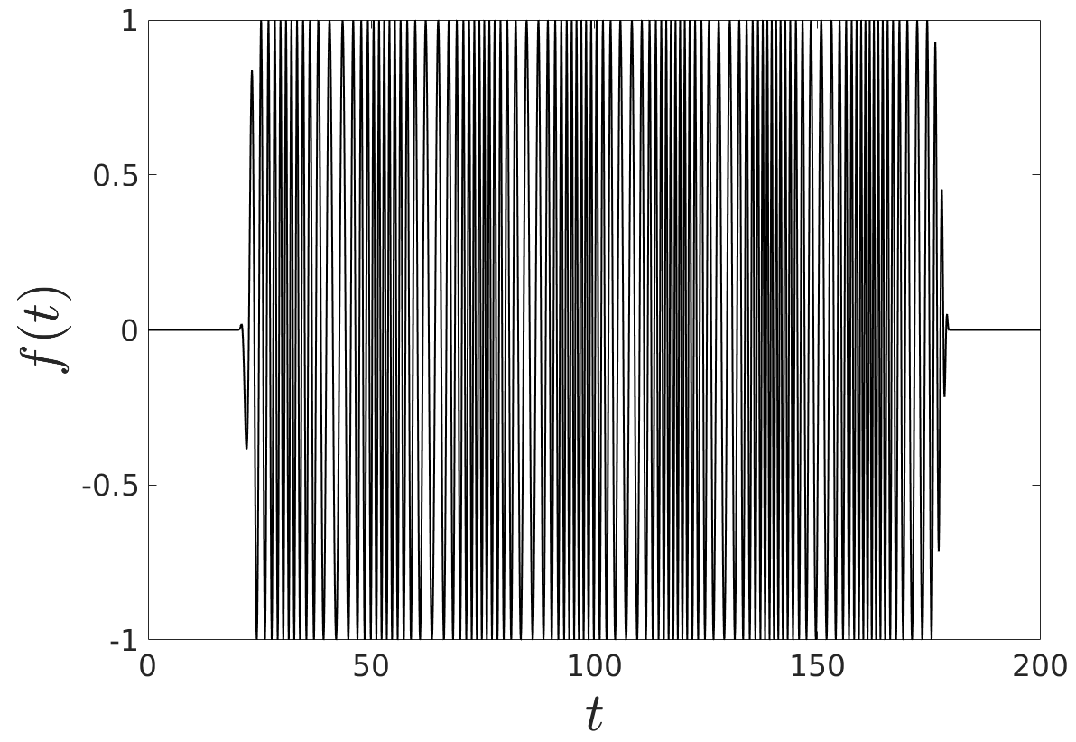
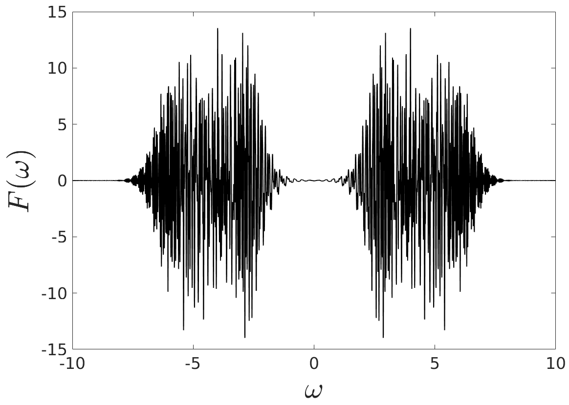
Figure 1: Left: Smooth, long duration time signal $f(t)$ as given in Eq. 44, windowed to have support in the interval $20\leq t\leq 180$. Right: Real part of the Fourier Transform $F(\omega)$ of $f(t)$. The Fourier transform $F(\omega)$ is highly oscillatory on account of the large $t$ values contained in the left-hand integrand in Eq. 11.

The proposed strategy for the large-$T$ Fourier transform problem is based on use of a partition-of-unity (POU) set $\mathcal{P}=\{w_{k}(t)\,|\,k=1,\dots,K\}$ of “well-spaced” windowing functions, where $w_{k}$ is supported in a neighborhood of the point $s=s_{k}$ for certain “support centers” $s_{k}\in[0,T]$ ($1\leq k\leq K$) satisfying, for some constants $H_{1},H_{2}>0$, the minimum-spacing property $s_{k+1}-s_{k}\geq H_{1}$, as well as the maximum width condition $w_{k}(t)=0$ for $|t-s_{k}|>H_{2}$ and the partition-of-unity relation $\sum_{k=1}^{K}w_{k}=1$. Setting $H=H_{1}=H_{2}$ in our test cases we use POU sets based on the following parameter selections

1. $s_{k+1}-s_{k}=3H/2$,

2. $w_{k}(t)=1$ in a neighborhood $|t-s_{k}|<H/2$,

3. $w_{k}(t)=0$ for $|t-s_{k}|>H$, and

4. $\sum_{k=1}^{K}w_{k}(t)=1\quad\mbox{for all}\quad t\in[0,T]$.

Note that, since $H$ is (or, more generally $H_{1}$ and $H_{2}$ are) $T$-independent, the integer $K$ is necessarily an $\mathcal{O}(T)$ quantity. In practice we use the prescription $w_{k}(t)=w(t-s_{k})$, with partition centers and window function given by $s_{k}=3(k-1)H/2$ (the parameter choice $H=10$ was used in all cases in this article) and

(12) $${\color[rgb]{0,0,0}w(t)}=\begin{cases}1-\eta({\color[rgb]{0,0,0}\frac{t+H}{H/2}}),&-H\leq t\leq-H/2\\ 1,&-H/2<t<H/2\\ \eta(\frac{t-H/2}{H/2}),&H/2\leq t\leq H\\ 0,&|t|>H,\end{cases}$$

respectively, where we use the smooth windowing function $\eta\in C_{c}^{\infty}([-1,1])$, $\eta(u)=\exp(\frac{2e^{-1/u}}{u-1})$.

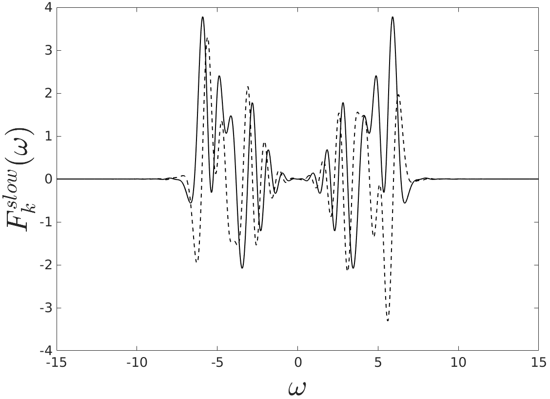
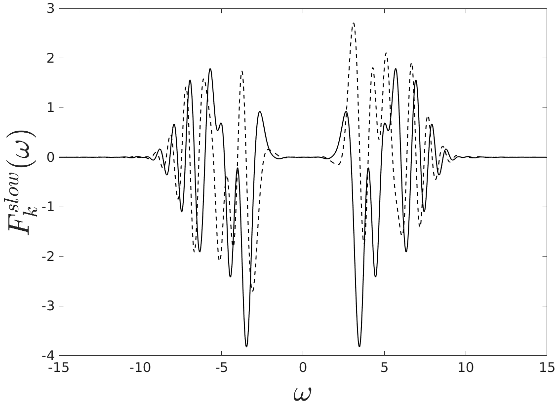
Figure 2: Fourier Transform of two windowed partitions of the long duration signal shown in Figure 1, each with partition width $H=10$. With reference to the text, the left and right figures depict the transform corresponding, respectively, to partition centers at $s_{k}=35$ ($k=4$) and $s_{k}=155$ ($k=16$). In each case, the solid and dashed traces depict the real and imaginary parts of the Fourier Transform, respectively. The transforms are both less than $10^{-4}$ outside the plotted region.

Using the partition of unity $\mathcal{P}$ and letting $f_{k}(t)=w_{k}(t)f(t)$, for $\omega\in[-W,W]$ we obtain the expression

(13) $$F(\omega)=\sum_{k=1}^{K}F_{k}(\omega),\quad\mbox{where}\quad F_{k}(\omega)=\int_{s_{k}-H_{2}}^{s_{k}+H_{2}}f_{k}(t){\mathrm{e}}^{{\mathrm{i}}\omega t}\,{\mathrm{d}}t,$$

which resembles the type of integrals used in connection with the windowed Fourier transform [37]. Now, centering the integration interval around the origin we obtain

(14) $$F_{k}(\omega)=\int_{-H_{2}}^{H_{2}}f_{k}(t+s_{k}){\mathrm{e}}^{{\mathrm{i}}\omega(t+s_{k})}\,{\mathrm{d}}t={\mathrm{e}}^{{\mathrm{i}}\omega s_{k}}F_{k}^{\textit{slow}}(\omega)$$

where

(15) $$F_{k}^{\textit{slow}}(\omega)=\int_{-H_{2}}^{H_{2}}f_{k}(t+s_{k}){\mathrm{e}}^{{\mathrm{i}}\omega t}\,{\mathrm{d}}t.$$

The “slow” superscript refers to the fact that, since $t$ in Eq. 15 is “small” (it satisfies $-H_{2}\leq t\leq H_{2}$), it follows that the integrand Eq. 15 only contains slowly oscillating exponential functions of $\omega$, and thus $F_{k}^{\textit{slow}}(\omega)$ is itself slowly oscillatory. Thus Eq. 14 expresses $F_{k}(\omega)$ as product of two terms: the (generically) highly oscillatory exponential term ${\mathrm{e}}^{i\omega s_{k}}$ (which arises for signals whose support center is away from the origin in time), on one hand, and the slowly oscillatory term $F_{k}^{\textit{slow}}(\omega)$, on the other. Fig. 2 displays the real and imaginary parts of $F_{k}^{\textit{slow}}$ for two values of $k$, namely $k=4$ and $k=16$. Note that despite the differing centers in time, the functions are similarly oscillatory and both are much less oscillatory than the Fourier transform depicted in Fig. 1.

Remark 3.

Since $f$ is smooth and compactly supported, iterated integration by parts in the integral expressions that define $F(\omega)$, $F_{k}(\omega)$ and $F_{k}^{\textit{slow}}(\omega)$ (equations Eq. 11, Eq. 14 and Eq. 15), and associated expressions for the derivatives of these functions of any positive order, shows that these functions and their derivatives decay as $1/\omega^{n}$ as $\omega\to\pm\infty$ for all $n>1$ for which $f\in C^{n}$. In other words, for smooth functions $f$ these three functions, along with each one of their derivatives respect to $\omega$ (of any order), decay superalgebraically fast as $\omega\to\pm\infty$. Additionally, in the two latter cases the superalgebraically fast decay (for each fixed order of differentiation) is uniform in $k$.

Remark 4.

Let $G:\mathbb{R}\to\mathbb{C}$, $G=G(\omega)$, denote a function that decays super-algebraically fast, along with each one of its derivatives, as $\omega\to\infty$. Then, repeated use of integration by parts on the inverse Fourier transform expression $g(t)=\frac{1}{2\pi}\int_{-\infty}^{\infty}G(\omega){\mathrm{e}}^{-{\mathrm{i}}\omega t}\,{\mathrm{d}}\omega$ shows that the error in the approximation

$$g(t)\approx\frac{1}{2\pi}\int_{-W}^{W}G(\omega){\mathrm{e}}^{-{\mathrm{i}}\omega t}\,{\mathrm{d}}\omega$$

decays super-algebraically fast as $W\to\infty$.

Remark 5.

Let $G=G(\omega)$ denote a superalgebraically-decaying function, as in Remark 4. Then, repeated use of integration by parts in the integral expressions for the Fourier coefficients $g_{n}$ shows that the expansion of $G$ as a $2W$-periodic Fourier series

$$G(\omega)\approx\sum_{n=-\infty}^{\infty}g_{n}{\mathrm{e}}^{{\mathrm{i}}{\color[rgb]{0,0,0}n}\pi\omega/W},\quad-W\leq\omega\leq W,$$

together with all of its derivatives, converge to $G(\omega)$ and its respective derivatives uniformly and super-algebraically fast, as $W\to\infty$, throughout the interval $[-W,W]$.

3.2 Windowed and re-centered wave equation and solutions with slow $\omega$ dependence

In order to evaluate numerically the solution of the problem Eq. 1 we apply the smooth time partitioning strategy developed in Section 3.1 to the boundary-condition function $b(\mathbf{r},t)$ in Eq. 1c (as a function of $t$ for each fixed value of $\mathbf{r}$). Thus, using the window functions $w_{k}(t)$ described in the previous section, we define two different types of windowed boundary-condition functions $b_{k}=b_{k}(\mathbf{r},t)$, namely 1) The function

(16) $$b_{k}(\mathbf{r},t)=w_{k}(t)b(\mathbf{r},t),$$

which can be used for general incident fields $b(\mathbf{r},t)$, as well as, 2) Specifically for incident fields of the form Eq. 3, the function

(17) $$b_{k}(\mathbf{r},t)=\frac{1}{2\pi}\int_{-\infty}^{\infty}B^{t}_{k}(\omega){\mathrm{e}}^{{\mathrm{i}}(\kappa(\omega)\mathbf{p}\cdot\mathbf{r}-\omega t)}\,{\mathrm{d}}\omega\quad\mbox{with}\quad\kappa(\omega)=\omega/c,$$

where, letting

(18) $$a_{k}(t)=w_{k}(t)a(t)$$

we have set

(19) $$B_{k}^{t}(\omega)=\int_{-\infty}^{\infty}a_{k}(t){\mathrm{e}}^{{\mathrm{i}}\omega t}\,{\mathrm{d}}t=\int_{-\infty}^{\infty}w_{k}(t)a(t){\mathrm{e}}^{{\mathrm{i}}\omega t}\,{\mathrm{d}}t.$$

Note that both definitions of $b_{k}(\mathbf{r},t)$ imply $\sum_{k=1}^{K}b_{k}(\mathbf{r},t)=b(\mathbf{r},t)$. In view of Remark 1 the present article uses the boundary condition function Eq. 17.

Letting $u_{k}(\mathbf{r},t)$ ($1\leq k\leq K$) denote the solution to Eq. 1 with boundary-condition function $b(\mathbf{r},t)$ substituted by $b_{k}(\mathbf{r},t)$, we clearly have

(20) $$u(\mathbf{r},t)=\sum_{k=1}^{K}u_{k}(\mathbf{r},t).$$

This expression is the basis of the time-domain solver proposed in this paper.

Remark 6.

As discussed extensively in Part II, in view of Huygens’ principle in three dimensions, and a certain windowing reallocation strategy in two dimensions, a fixed, geometry-dependent, number $M$ (independent of $K=\mathcal{O}(T)$) of solutions $u_{k}$ need to be included for any space-time evaluation region, irrespective of the time duration $T$ for which the solution is evaluated. The geometry-dependence of the parameter $M$ relates closely to the trapping character [48, 49] of the underlying scattering geometry; while $M$ may grow large for slowly-decaying scattered fields, the finite-duration character of the incident field is guaranteed by this theory to yield an overall-bounded number of active partitions. This is the basis of tracking strategies for identifying the “active” time-partition solutions, which will be presented elsewhere. Figure 5, which displays the computed functions $u_{k}$ for $k=1,2,3$, and in which the solution for each partition is only plotted if it exceeds a certain tolerance anywhere in the entire domain of interest, illustrates, in a rudimentary fashion, some of the principles inherent in those strategies.

Accurate numerical approximations of the solutions $u_{k}$ can be produced as indicated in what follows. Considering the boundary condition function $b_{k}(\mathbf{r},t)$ in Equation 17, Equations Eq. 13 and Eq. 15 yield

(21) $$B^{t}(\omega)=\sum_{k=1}^{K}B^{t}_{k}(\omega),\quad\mbox{and}\quad B^{t}_{k}(\omega)={\mathrm{e}}^{{\mathrm{i}}\omega s_{k}}B_{k}^{\textit{slow}}(\omega).$$

Thus, denoting by $U^{t}_{k}(\mathbf{r},\omega)$ and $U_{k}^{\textit{slow}}(\mathbf{r},\omega)$ the frequency domain solutions of the problem Eq. 2 with $B^{t}$ replaced by $B^{t}_{k}(\omega){\mathrm{e}}^{{\mathrm{i}}\kappa(\omega)\mathbf{p}\cdot\mathbf{r}}$ and $B_{k}^{\textit{slow}}(\omega){\mathrm{e}}^{{\mathrm{i}}\kappa(\omega)\mathbf{p}\cdot\mathbf{r}}$, respectively, we obtain the representations

(22) $$u_{k}(\mathbf{r},t)=\frac{1}{2\pi}\int_{-\infty}^{\infty}U^{t}_{k}(\mathbf{r},\omega){\mathrm{e}}^{-{\mathrm{i}}\omega t}\,{\mathrm{d}}\omega=\frac{1}{2\pi}\int_{-\infty}^{\infty}U_{k}^{\textit{slow}}(\mathbf{r},\omega){\mathrm{e}}^{-{\mathrm{i}}\omega(t-s_{k})}\,{\mathrm{d}}\omega.$$

Since $U_{k}^{\textit{slow}}$ is approximately band-limited (because $B_{k}^{\textit{slow}}$ is, see Remark 3), it follows from Eq. 22 and Remark 4 that $u_{k}(\mathbf{r},t)$ can be approximated by the strictly band-limited function $u_{k}^{W}$:

(23) $$u_{k}(\mathbf{r},t)\approx u_{k}^{W}(\mathbf{r},t)=\frac{1}{2\pi}\int_{-W}^{W}U_{k}^{\textit{slow}}(\mathbf{r},\omega){\mathrm{e}}^{-{\mathrm{i}}\omega(t-s_{k})}\,{\mathrm{d}}\omega$$

with superalgebraically small errors (uniform in $\mathbf{r}$, $t$ and $k$) as the bandwidth $W$ grows.

Section 4 presents a quadrature algorithm that, on the basis of a finite set of frequencies $\mathcal{F}=\{\omega_{j}:\,j=1,\dots,J\}$, approximates, with errors uniform-in-$t$ and decaying rapidly as $J$ increases, the highly-oscillatory integral Eq. 23, and thus produces the numerical approximation $u_{k}^{W,J}\approx u_{k}^{W}$, by means of spectral interpolation of the slowly-varying quantity $U_{k}^{\textit{slow}}(\cdot,\omega)$ with respect to $\omega$. The quantity $U_{k}^{\textit{slow}}$, in turn, is dependent on frequency-domain incident data $B_{k}^{\textit{slow}}$ obtained (via use of the numerical transform techniques introduced in Section 4.1 for the function $a_{k}=w_{k}a$) from the relation

(24) $$B_{k}^{\textit{slow}}(\omega)=\int_{-H}^{H}a_{k}(t+s_{k}){\mathrm{e}}^{{\mathrm{i}}\omega t}\,{\mathrm{d}}t,$$

and boundary integral “scattering” densities $\psi_{\mathbf{p}}^{t}$ , where $\psi_{\mathbf{p}}^{t}$ are solutions of Equation 10 with $B^{t}$ replaced by ${\mathrm{e}}^{{\mathrm{i}}\kappa(\omega)\mathbf{p}\cdot\mathbf{r}}$. Specifically, defining

(25) $$\psi_{k}^{\textit{slow}}(\mathbf{r}^{\prime},\omega)=B_{k}^{\textit{slow}}(\omega)\psi_{\mathbf{p}}^{t}(\mathbf{r}^{\prime},\omega),$$

for the time-partition-specific boundary density we have

(26) $$\begin{split}U_{k}^{\textit{slow}}(\mathbf{r},\omega)=\int_{\Gamma}\psi_{k}^{\textit{slow}}(\mathbf{r}^{\prime},\omega)&G_{\omega}(\mathbf{r},\mathbf{r}^{\prime})\,{\mathrm{d}}\sigma(\mathbf{r}^{\prime})\\ &=B_{k}^{\textit{slow}}(\omega)\int_{\Gamma}\psi_{\mathbf{p}}^{t}(\mathbf{r}^{\prime},\omega)G_{\omega}(\mathbf{r},\mathbf{r}^{\prime})\,{\mathrm{d}}\sigma(\mathbf{r}^{\prime}).\end{split}$$

It follows that for a given bandwidth $W$ all the needed function values $U_{k}^{\textit{slow}}(\mathbf{r},\omega_{j})$ can be produced in terms of the fixed ($k$-independent, $W$-dependent) finite set $\Psi=\{\psi^{t}_{\mathbf{p}}(\cdot,\omega_{j}):\,j=1,\dots,J\}$ of boundary integral densities. The re-utilization of the fixed ($k$-independent) set $\Psi$ of “expensive” integral densities is a crucial element leading to the efficiency of the overall hybrid algorithm.

4 FFT-based $\mathcal{O}(1)$-cost Fourier transform at large times

This section presents an effective algorithm for the numerical evaluation of truncated Fourier integrals of the form

(27) $$F(\omega)=\int_{-H}^{H}f(t){\mathrm{e}}^{{\mathrm{i}}\omega t}\,{\mathrm{d}}t\quad\mbox{and}\quad f(t)=\frac{1}{2\pi}\int_{-W}^{W}F(\omega){\mathrm{e}}^{-{\mathrm{i}}\omega t}\,{\mathrm{d}}\omega$$

(cf. Equations Eq. 15 and Eq. 23), at arbitrarily large evaluation arguments $t$ and $\omega$. Here, it is assumed that $f$ is a smooth function of time $t\in\mathbb{R}$ which vanishes outside the interval $[-H,H]$. Similarly, with the possible exception of a inverse-logarithmic singularity of $F(\omega)$ at $\omega=0$ for certain two-dimensional applications (see Section 4.2), $F$ is an infinitely smooth function for all frequencies $\omega$—which is additionally superalgebraically small outside the interval $[-W,W]$. The case in which a singularity exists in Equation 27 at $\omega=0$ is handled in Section 4.2 by utilizing a decomposition of the form

(28) $$f(t)=\left(\int_{-W}^{-w_{c}}+\int_{-w_{c}}^{w_{c}}+\int_{w_{c}}^{W}\right)F(\omega){\mathrm{e}}^{-{\mathrm{i}}\omega t}\,{\mathrm{d}}\omega,$$

together with a specialized quadrature rule for the middle integral; the function $F$ is smooth (though not necessarily periodic) in the integration intervals $[-W,-\omega_{c}]$ and $[\omega_{c},W]$.

Use of trapezoidal rule integration might appear advantageous in these contexts, since, for such boundary-vanishing integrands the trapezoidal rule exhibits superalgebraically fast convergence (at least in the smooth $F$ case), and, importantly, unlike the Gauss-Hermite rule used in [47], it can be efficiently evaluated by means of FFTs. However, as the evaluation arguments $t$ or $\omega$ grow, the integrands in Eq. 27 become more and more oscillatory. Both the Gauss-Hermite and the trapezoidal rule (and, indeed, any quadrature rule based on standard interpolation techniques) require use of finer and finer meshes to avoid completely inaccurate approximations as the evaluation argument increases (see Section 3.1). Failure to resolve this difficulty would lead to a fundamental breakdown in the algorithm—as it would be necessary for the scheme to produce an increasing number of (expensive) boundary integral equation solutions, leading to rapidly increasing costs, as evaluation times grow.

Remark 7.

For definiteness, the presentation in this section is restricted to the right-hand integral in Eq. 27; the corresponding algorithm for the left-hand integral is entirely analogous.

Remark 8.

A direct examination of the trapezoidal approximation

(29) $$f(t)=\frac{1}{2\pi}\int_{-W}^{W}F(\omega){\mathrm{e}}^{-{\mathrm{i}}t\omega}\,{\mathrm{d}}\omega\approx\frac{W}{2\pi m}\sum_{k=0}^{m-1}F(\omega_{k}){\mathrm{e}}^{-{\mathrm{i}}t\omega_{k}}\quad\left(\omega_{k}=-W+k\,\Delta\omega\right)$$

shows that, as is well known, quadrature errors in the trapezoidal quadrature rule for “large” $t$ manifest themselves as “aliasing”, that is, spurious periodicity in the $t$ variable [5, 34, 36, 44].

The method proposed in the present Section 4 resolves the difficulties mentioned in the last paragraph: it eliminates aliasing errors without recourse to frequency mesh refinement, and it evaluates (on the basis of FFTs) the time-domain solution in constant computing time per temporal evaluation point—so that, as in finite-difference time-marching algorithms, the overall cost per timestep of the time propagation algorithm does not grow as time increases.

4.1 Smooth $F(\omega)$: FFT-based reduction to “scaled convolution”

This section considers the problem of evaluation of Fourier integrals similar to those in Eq. 27 (or, in 2D contexts, the integrals with smooth integrands in Equation 28) under the assumption that the functions $f$ and $F$ are infinitely smooth in the domain of integration. In the context of Equation 23 in dimension $d=3$ the smoothness assumption on $F$ is always satisfied, as it is for dimension $d=2$ provided that, e.g., $F(\omega)=U_{k}^{\textit{slow}}(\mathbf{r},\omega){\mathrm{e}}^{{\mathrm{i}}\omega s_{k}}$ vanishes in a neighborhood of $\omega=0$. The singular $d=2$ case is tackled in Section 4.2.

The proposed smooth-$F$ approach proceeds by trigonometric-series expansion of the integrand function $F$ followed by use of certain “scaled convolutions” introduced in Section 4.1.1; a fast FFT-based algorithm for evaluation of such convolution-like quantities is then described in Section 4.1.2.

4.1.1 Transform approximation via Fourier Series expansion

In this Section we develop a quadrature rule for the general transform integral

(30) $$I_{a}^{b}\,[F](t)=\int_{a}^{b}F(\omega){\mathrm{e}}^{-{\mathrm{i}}\omega t}\,{\mathrm{d}}\omega,$$

or, equivalently,

(31) $$I_{a}^{b}\,[F](t)={\mathrm{e}}^{-{\mathrm{i}}\delta t}\int_{-A}^{A}F(\delta+\omega){\mathrm{e}}^{-{\mathrm{i}}\omega t}\,{\mathrm{d}}\omega,\quad\mbox{where}\quad A=\frac{b-a}{2}\quad\mbox{and}\quad\delta=\frac{b+a}{2}.$$

Although $F(\delta+\omega)$ may not be a periodic function of $\omega$ in the integration interval $[-A,A]$, for a prescribed positive even integer $M$ we utilize a trigonometric polynomial of the form

(32) $$F(\delta+\omega)\approx\sum_{m=-\nicefrac{{M}}{{2}}}^{\nicefrac{{M}}{{2}}-1}c_{m}{\mathrm{e}}^{{\mathrm{i}}\frac{2\pi}{P}m\omega}$$

of a certain periodicity $P$, that closely approximates $F(\delta+\omega)$ for $\omega\in[-A,A]$.

Remark 9.

As indicated below, in the context of this paper $F(\delta+\omega)$ is most often a smoothly periodic function in $[-A,A]$ (with $A$ equal to the bandlimit $W$); in such cases we take $P=2A$ and (32) is obtained as a regular Discrete Fourier Transform (DFT) in $[-A,A]$. Exceptions do arise in certain two-dimensional situations (Section 4.2) where $F(\delta+\omega)$ is smooth but not periodic in $[-A,A]$ (cf. the first and last integrals in Eq. 28); in such cases an accurate Fourier approximation of a certain period $P\neq 2A$ is obtained in our algorithm on the basis of the FC(Gram) Fourier Continuation method [22, 1]. In the periodic case the errors inherent in the approximation Eq. 32 tend to zero super-algebraically fast (faster than any negative power of $M$ [2, Lemma 7.3.3], cf. also Remark 5), while the errors arising from the Fourier Continuation method used in the non-periodic case decay as a user-prescribed negative power of $M$.

Substituting Eq. 32 into Eq. 31 and integrating term-wise yields the approximation

(33) $$\begin{split}I_{a}^{b}\,[F](t)&\approx{\mathrm{e}}^{-{\mathrm{i}}\delta t}\sum_{m=-\nicefrac{{M}}{{2}}}^{\nicefrac{{M}}{{2}}-1}c_{m}\int_{-A}^{A}{\mathrm{e}}^{-{\mathrm{i}}\frac{2\pi}{P}(\alpha t-m)\omega}\,{\mathrm{d}}\omega\\ &={\mathrm{e}}^{-{\mathrm{i}}\delta t}\sum_{m=-\nicefrac{{M}}{{2}}}^{\nicefrac{{M}}{{2}}-1}c_{m}\frac{P}{\pi(\alpha t-m)}\sin\left(\pi\frac{2A}{P}(\alpha t-m)\right),\end{split}$$

where we have set $\alpha=\frac{P}{2\pi}$. In view of Eq. 33, for a given user-prescribed (!) equi-spaced time-evaluation grid $\left\{t_{n}=n\Delta t\right\}_{n=N_{1}}^{N_{2}}$ we may write, letting $\beta=\alpha\Delta t$,

(34) $$I_{a}^{b}\,[F](t_{n})\approx{\mathrm{e}}^{-{\mathrm{i}}\delta t_{n}}\sum_{m=-\nicefrac{{M}}{{2}}}^{\nicefrac{{M}}{{2}}-1}c_{m}b_{\beta n-m},\quad\mathrm{where}\quad b_{q}\coloneqq 2A\operatorname{sinc}\left(\frac{2A}{P}q\right).$$

Note that, paralleling the fast Fourier series convergence in the periodic case, equations Eq. 33 and Eq. 34 provide super-algebraically close approximations of $I_{a}^{b}[F](t)$. In the non-periodic case, these equations provide a user-prescribed algebraic order of accuracy. In either case, the errors in Eq. 33 and Eq. 34 are uniform in $t$ and $n$, respectively: for a given error tolerance $\varepsilon$ there exists an integer $M_{0}$ (independent of $t$ and $t_{n}$) such that, for all $M\geq M_{0}$, the approximation errors in Eq. 33 and Eq. 34 are less than $\varepsilon$ for all $t\in\mathbb{R}$ and all relevant values $t_{n}$, respectively.

Remark 10.

It is useful to note that the aforementioned $t$- and $t_{n}$-independent errors in Eq. 33 and Eq. 34 stem solely from corresponding errors in the expansion Eq. 32—and thus, can be achieved on the basis of values of the function $F(\delta+\omega)$ on a fixed ($t$-independent) finite set $\mathcal{F}^{\textrm{smooth}}$ of frequency mesh points, cf. Section 5.

Since generically $\beta\neq 1$ (indeed, $\beta\not\in\mathbb{Z}$ generically), the quantity $\sum_{m}c_{m}b_{\beta n-m}$ in Eq. 34 is not a discrete convolution, but it is, rather, a “discrete scaled convolution” [50]. Like regular discrete convolutions, scaled convolutions can accurately be produced by means of FFTs [50]—although the algorithm for scaled convolutions is somewhat more complicated than the standard FFT convolution approach. Still, the fast scaled convolution algorithm is a useful tool: it runs in $\mathcal{O}(L\log L)$ operations (where $L=\mathrm{max}(N_{2}-N_{1},M)$) and it produces highly accurate results; details are presented in Section 4.1.2.

4.1.2 FFT accelerated evaluation of scaled discrete convolutions

The quadrature method introduced in Section 4.1.1 reduces the evaluation of the right-hand transform in Eq. 27 for values $t=t_{n}$ (for a given range $0\leq n-n_{0}\leq N-1$ with $n_{0}\in\mathbb{Z}$ and $N\in\mathbb{N}$) to evaluation of scaled convolutions of the form

(35) $$d_{n}=\sum_{m=-\nicefrac{{M}}{{2}}}^{\nicefrac{{M}}{{2}}-1}c_{m}b_{\beta m-\gamma n},\quad 0\leq n-n_{0}\leq N-1,$$

where the coefficients $c_{m}$ are complex numbers that make up a certain “input vector” $\vec{c}=(c_{-M/2},\dots,c_{-M/2-1})$, and where the “convolution kernel” $b$ is a function of its real-valued sub-index $q$: $b_{q}=b(q)$. (Compare Eq. 34 and Eq. 35 and note the specific scaled convolution kernel $b_{q}$ and parameter value $\gamma=1$ used in the former equation.) This section presents an algorithm which evaluates the sum Eq. 35 for all required values of $n$ at FFT speeds.

To describe the algorithm, let $L$ denote a certain positive even integer, to be defined below, which is larger than or equal to the maximum of $N$ and $M$. The convolution input vector $\vec{c}$ is symmetrically zero-padded to form a new vector $\vec{c}=(c_{-L/2},c_{-L/2+1},\dots,c_{L/2-1})$ of length $L$. New elements are also added to the list of evaluation indices in Eq. 35 so that the overall list contains the $L$ elements in the indicial vector $\vec{n}=(n_{0}-L/2,n_{0}-L/2+1,\dots,n_{0}+L/2-1)$. Following [50], for technical reasons the length $L$ is determined by the relation $L\geq L_{0}$, where $L_{0}$ denotes the smallest even integer for which the kernel index parameter $q=\beta m-\gamma n$ lies in the range $-L_{0}/2\leq q\leq L_{0}/2-1$ for $-M/2\leq m\leq M/2-1$, $0\leq n-n_{0}\leq N-1$. (As pointed out below, selections satisfying $L>L_{0}$ are occasionally necessary to achieve a prescribed error tolerance.) In view of these selections, the scaled convolution expression (35) is embedded in the analogous but more favorably structured convolution expression

(36) $$d_{n}=\sum_{m=-\nicefrac{{L}}{{2}}}^{\nicefrac{{L}}{{2}}-1}c_{m}b_{\beta m-\gamma n},\quad-L/2\leq n-n_{0}\leq L/2-1,$$

Using the $\gamma$-fractional discrete Fourier transform $C_{p}^{(\gamma)}$ (that is to say, the fractional Fourier transform based on roots of unity parameter $\gamma$ as in [4]) together with the discrete Fourier transform $B_{p}$,

$$C_{p}^{(\gamma)}=\sum_{m=-\nicefrac{{L}}{{2}}}^{\nicefrac{{L}}{{2}}-1}c_{m}{\mathrm{e}}^{-{\mathrm{i}}\frac{2\pi\gamma mp}{L}},\quad B_{p}=\sum_{m=-\nicefrac{{L}}{{2}}}^{\nicefrac{{L}}{{2}}-1}b_{m}{\mathrm{e}}^{-{\mathrm{i}}\frac{2\pi mp}{L}},$$

an application of the convolution theorem yields [50]

(37) $$d_{n}=\sum_{m=-\nicefrac{{L}}{{2}}}^{\nicefrac{{L}}{{2}}-1}c_{m}b_{\beta m-\gamma n}\approx\frac{1}{L}\sum_{p=-\nicefrac{{L}}{{2}}}^{\nicefrac{{L}}{{2}}-1}C_{p}^{(\gamma)}B_{p}{\mathrm{e}}^{{\mathrm{i}}\frac{2\pi\beta np}{L}},\quad-L/2\leq n-n_{0}\leq L/2-1,$$

reducing, in particular, the (approximate) evaluation of the desired values $d_{n}$ in (35) to evaluation of a discrete Fourier transform and a $\gamma$-fractional discrete Fourier transform, both of size $L$, followed by evaluation of the $L$-term inverse $\beta$-fractional Fourier transform on the right-hand side of Eq. 37. The necessary discrete Fourier transform can of course be evaluated by means of the FFT algorithm. The fractional Fourier transforms (FRFTs) can also be accelerated on the basis of the FFT-based fractional Fourier transform algorithms, at an $\mathcal{O}(L\log L)$ cost of approximately four times that of an $L$-point FFT; see [4]. The error inherent in the approximation Eq. 37 is a quantity of order $\mathcal{O}(L^{-2})$, which, in our applications, generally yields any desired accuracy in very fast computing times by selecting appropriate values of the parameter $L$.

$M$	Direct (s)	Fast (s)	$\varepsilon^{\mathrm{Fast}}$
$10^{1}$	$5.6\cdot 10^{-2}$	$8.3\cdot 10^{-3}$	$6.6\cdot 10^{-3}$
$10^{2}$	$8.3\cdot 10^{-2}$	$7.9\cdot 10^{-3}$	$1.9\cdot 10^{-7}$
$10^{3}$	$1.8\cdot 10^{-1}$	$7.8\cdot 10^{-3}$	$1.6\cdot 10^{-8}$
$10^{4}$	$1.4\cdot 10^{0}$	$8.2\cdot 10^{-3}$	$7.9\cdot 10^{-7}$

$N$	Direct (s)	Fast (s)	$\varepsilon^{\mathrm{Fast}}$
$10^{1}$	$1.5\cdot 10^{-3}$	$1.1\cdot 10^{-2}$	$6.2\cdot 10^{-6}$
$10^{2}$	$1.2\cdot 10^{-2}$	$7.5\cdot 10^{-3}$	$5.8\cdot 10^{-6}$
$10^{3}$	$8.8\cdot 10^{-2}$	$8.1\cdot 10^{-3}$	$4.7\cdot 10^{-6}$
$10^{4}$	$7.1\cdot 10^{-1}$	$8.0\cdot 10^{-3}$	$2.6\cdot 10^{-7}$
$10^{5}$	$7.5\cdot 10^{0}$	$9.3\cdot 10^{-2}$	$2.1\cdot 10^{-9}$
$10^{6}$	$9.4\cdot 10^{1}$	$1.5\cdot 10^{0}$	$2.6\cdot 10^{-10}$
$10^{7}$	$2.8\cdot 10^{3}$	$2.3\cdot 10^{1}$	$5.5\cdot 10^{-9}$

Table 1: Computing times required for evaluation of the size-$M$ scaled convolution Eq. 34 by means of the Direct and Fast algorithms described in the text at a number $N$ of time points $t_{n}$, and errors $\varepsilon^{\mathrm{Fast}}$ associated with the Fast algorithm. (By definition, the Direct algorithm provides the exact convolution results, up to roundoff.) Left: $N=10^{4}$. Right: $M=5000$.

To demonstrate the accelerated scaled-convolution algorithm we evaluate the transform (35) for several values of $N$, with certain coefficients $c_{m}$ ($-M/2\leq m\leq M/2-1$) and with $b_{q}$ as in (34). (The particular selection of the coefficients $c_{m}$ is immaterial in the context of the present demonstration, but, for reference, we mention that the coefficients used in the example were obtained as the coefficients of the $M$-term FC expansion Eq. 32 with $F(\omega)={\mathrm{e}}^{-\frac{1}{4}(\omega-10)^{2}}{\mathrm{e}}^{-{\mathrm{i}}8\omega}$ in the interval $[8,15]$. This specific scaled convolution arises as the method in Section 4.1.1 is applied to the evaluation of Eq. 30 on $[0,T]$, with $T=N\Delta t$ and $\Delta t=0.2$.) Letting $\widetilde{d}_{n}$ denote the approximation of $d_{n}$ produced by the fast algorithm, Table 1 displays the $\ell^{\infty}$ error $\varepsilon^{\mathrm{Fast}}=\mathrm{max}_{n}|d_{n}-\widetilde{d}_{n}|$ as well as the time required by the fast method to produce the $M$-coefficient sum at the required $N$ evaluation points. The computations were performed in MATLAB on an Intel Core i7-8650U CPU.

4.2 Non-smooth $F(\omega)$: singular quadrature for 2D low frequency scattering

This section concerns the evaluation of the inverse transform in Eq. 27 for cases in which $F$ contains an (integrable) singularity at $\omega=0$. In the context of the proposed wave equation solver, this occurs in the evaluation of Eq. 23 in the $d=2$ case (where for each spatial point $\mathbf{r}$ we have $F(\omega)=U_{k}^{\mathrm{slow}}(\mathbf{r},\omega){\mathrm{e}}^{{\mathrm{i}}\omega s_{k}}$) since, as is known [46, 57], in two dimensions the solutions to the Helmholtz equation vary as an integrable function of $\log\omega$ which vanishes at $\omega=0$. (Special treatments are not necessary in the $d=3$ case, where, given incident fields with smooth $\omega$-dependence, the Helmholtz solutions vary smoothly with $\omega$ for all real values of $\omega$ [56, 41].)

To design our quadrature rule in the non-smooth case we recall the decomposition Eq. 28,

(38) $$f(t_{\ell})=\left(\int_{-W}^{-w_{c}}+\int_{-w_{c}}^{w_{c}}+\int_{w_{c}}^{W}\right)F(\omega){\mathrm{e}}^{-{\mathrm{i}}\omega t_{\ell}}\,{\mathrm{d}}\omega\eqqcolon I_{-}(t_{\ell})+I_{0}(t_{\ell})+I_{+}(t_{\ell}),$$

where using the notation introduced in Eq. 30, $I_{-}(t_{\ell})=I_{-W}^{-w_{c}}[F](t_{\ell})$ and $I_{+}(t_{\ell})=I_{w_{c}}^{W}[F](t_{\ell})$ can be treated effectively by means of the Fourier-based quadrature method developed in Section 4.1. Unfortunately, an application of that approach to $I_{0}(t_{\ell})=I_{-w_{c}}^{w_{c}}[F](t_{\ell})$ would not give rise to high-order accuracy, in view of the slow convergence of the Fourier expansion of $F$ in the interval $[-w_{c},w_{c}]$—that arises from the singularity of $F$ at $\omega=0$. We therefore develop a special quadrature rule for evaluation of the half-interval integral

(39) $$I_{0}^{\omega_{c}}\,[F](t)=\int_{0}^{\omega_{c}}F(\omega){\mathrm{e}}^{-{\mathrm{i}}t\omega}\,{\mathrm{d}}\omega$$

that retains the main attractive features of the integration methods developed in the previous section: high-order quadrature at fixed cost for evaluation at arbitrarily large times $t$.

Remark 11.

As in Section 4.1, the aforementioned $t$-independent errors can be achieved on the basis of fixed ($t$-independent) finite set, which will be denoted by $\mathcal{F}^{\textrm{sing}}$ in the present context, of frequency mesh points. The procedure used here, however, does not rely on Fourier approximation of $F$, cf. Remark 10.

In order to evaluate the Fourier integral $I_{0}(t_{\ell})$ at fixed cost for arbitrarily large times $t_{\ell}$, despite the presence of increasingly oscillatory behavior of the transform kernel, we rely on a certain modified “Filon-Clenshaw-Curtis” high-order quadrature approach [29] for non-smooth $F(\omega)$. The classical Filon-Clenshaw-Curtis method [54], which assumes a smooth function $F$, involves replacement of $F$ by its polynomial interpolant $Q_{\mathscr{N}}F$ at the Clenshaw-Curtis points followed by exact computation of certain associated “modified moments” (which are given by integrals of the Chebyshev polynomials multiplied by the oscillatory Fourier kernel). Importantly, this classical procedure eliminates the need to interpolate the target transform function at large numbers of frequency points as time increases. Additionally, on account of the selection of Clenshaw-Curtis interpolation points, the polynomial interpolants coincide with rapidly convergent Chebyshev approximations, and, therefore, the integration procedure converges with high-order accuracy. The accuracy resulting from use of a Chebyshev-based approach, which is very high for any value of $t$, actually improves as time increases: as shown in [29], the error in the method [54] asymptotically decreases to zero as $t\rightarrow\infty$.

The modified Filon-Clenshaw-Curtis method [29] we use in the present non-smooth-$F$ case (where $F$ is singular at $\omega=0$ only) proceeds on the basis of a graded set

(40) $$\Pi_{\mathscr{M},q}\coloneqq\left\{\mu_{j}\coloneqq\omega_{c}\left(\frac{j}{\mathscr{M}}\right)^{q}:j=1,\ldots,\mathscr{M}\right\},$$

of points in $(0,\omega_{c}]$ which are used to form subintervals $(\mu_{j},\mu_{j+1})$ ($1\leq j\leq\mathscr{M}-1$). For a given meshsize $\mathscr{N}$, each one of these subintervals is then discretized by means of a Clenshaw-Curtis mesh containing $\mathscr{N}$ points, and all of these meshes are combined in a single mesh set $\mathcal{F}^{\textrm{sing}}$ (which contains a total of $|\mathcal{F}^{\textrm{sing}}|=2(\mathscr{M}-1)\mathscr{N}$ points) that is to be used for evaluation of the integral $I_{0}$. Using this mesh, the Clenshaw-Curtis quadrature rule is applied to the evaluation of $I_{\mu_{j}}^{\mu_{j+1}}\,[F](t)$ (see Equation 30). The integral $I_{0}^{\omega_{c}}\,[F](t)$ is finally approximated by a composite quadrature rule that mirrors the exact relation

(41) $$I_{0}^{\omega_{c}}\,[F](t)=\sum_{j=2}^{\mathscr{M}}I_{\mu_{j-1}}^{\mu_{j}}\,[F](t).$$

The error introduced by this quadrature rule is discussed extensively in [29], and is of course dependent on the strength of the singularity. Briefly, in our context, and assuming $q>\mathscr{N}+1$, the convergence order as $\mathscr{N}\to\infty$ is determined by the number $\mathscr{M}$ of integration subintervals used: letting $I_{\mathscr{N}}\approx I$ denote the approximate value produced by the composite quadrature rule using $\mathscr{N}$ Clenshaw-Curtis points per subinterval, we find the error in $I_{\mathscr{N}}$ satisfies [29, Thm. 3.6]

$$|I[F]-I_{\mathscr{N}}[F]|=\mathcal{O}(\mathscr{M}^{-(1+\mathscr{N})})\quad\mbox{as}\quad\mathscr{N}\to\infty.$$

Whenever necessary (i.e. for two-dimensional problems containing nonzero content at zero-frequency), the numerical results presented in Section 6 were produced using the values $\mathscr{M}=4$, $\mathscr{N}=8$ and $q=9.1>\mathscr{N}+1$. Of course, two dimensional problems whose frequency spectrum is bounded away from the origin, and three-dimensional problems (which always enjoy a smooth frequency dependence even around $\omega=0$), do not require the use of the quadrature rule described above. The computational cost of this algorithm does not grow with increasing evaluation time $t$, consistent with the $\mathcal{O}(1)$ large time sampling cost for the overall hybrid method.

5 Fast-hybrid wave equation solver: overall algorithm description

Utilizing a number of concepts presented in the previous sections and additional notations, including

• An incident field $b$ of the form Eq. 3 for a given direction $\mathbf{p}$;

• A set $\mathcal{F}=\{\omega_{1},\dots,\omega_{J}\}$ of frequencies (n.b. $\mathcal{F}=\mathcal{F}^{\textrm{smooth}}\cup\mathcal{F}^{\textrm{sing}}$ in the 2D case, and $\mathcal{F}=\mathcal{F}^{\textrm{smooth}}$ in the 3D case, cf. Remark 10 and Remark 11)) used to discretize both the slow $H$-windowed Fourier transform $B_{k}^{\textit{slow}}$ (cf. Eq. 24) and the corresponding slow frequency scattered fields $U_{k}^{\textit{slow}}$ (cf. Eq. 26);

• A set $\mathcal{C}$ (of cardinality $N_{\Gamma}$) of scattering-boundary discretization points;

• Sets $\mathcal{R}$ (of cardinality $N_{\mathbf{r}}$) and $\mathcal{T}=\left\{t_{\ell}:\,1\leq\ell\leq N_{t}\right\})$ (of cardinality $N_{t}$) of discrete spatial and temporal observation points at which the scattered field is to be produced;

the single-incidence (see Remark 1)) time-domain algorithm introduced in this contribution is summarized in the following prescriptions.

1. Evaluate numerically the windowed incident-field signal functions $w_{k}(t)a(t)$, in Eq. 18 ($k=1,\dots,K$), over a temporal mesh adequate for evaluation of the Fourier transforms mentioned in Step [F2].

2. Obtain the boundary condition functions $B_{k}^{\textit{slow}}(\omega)$ at frequency mesh values $\omega=\omega_{j}\in\mathcal{F}$ ($1\leq j\leq J$) by Fourier transformation of the windowed signals in [F1], in accordance to Eq. 24.

3. Solve a total of $J$ integral equations Eq. 10 under plane-wave incidence with incidence vector $\mathbf{p}$ (see Remark 1) at the frequencies $\omega_{j}\in\mathcal{F}$, to produce, for each $j$, boundary integral densities $\psi^{t}=\psi^{t}_{\mathbf{p}}(\mathbf{r}^{\prime},\omega_{j})$, $\mathbf{r}^{\prime}\in\mathcal{C}$.

4. For each partition index $k=1,\dots,K$ produce the frequency-domain scattering boundary integral density $\psi_{k}^{\textit{slow}}$ with support in $[-W,W]$ on the basis of the densities $\psi^{t}_{\mathbf{p}}$ via an application of Equation 25.

5. Complete the frequency domain portion of the algorithm by evaluating, at each point $\mathbf{r}\in\mathcal{R}$, the frequency-domain solution $U_{k}^{\textit{slow}}(\mathbf{r},\omega_{j})$ in Equation 26 by numerical evaluation of the layer potential integral in that equation, using the density values $\psi_{k}^{\textit{slow}}(\mathbf{r}^{\prime},\omega_{j})$ at boundary points $\mathbf{r}^{\prime}\in\mathcal{C}$.

In order to evaluate the solution $u$ for all points in the set $\mathcal{R}$, and for all times in the set $\mathcal{T}$, the algorithm proceeds by transforming each windowed solution back to the time domain using the quadrature methods presented in Section 4. The following prescriptions thus complete the overall hybrid solver.

1. For $k=1$ to $K$ and For each $\mathbf{r}\in\mathcal{R}$ do:

2. 1. (3D case) Obtain the coefficients $c_{m}=c_{m}(\mathbf{r})$ of the Fourier series expansions of the form Eq. 32 for the functions $F(\omega)=U_{k}^{\textit{slow}}(\mathbf{r},\omega)$ in the interval $\omega\in[-W,W]$.

   2. (2D case) Obtain the coefficients $c_{m}^{(1)}=c_{m}^{(1)}(\mathbf{r})$ and $c_{m}^{(2)}=c_{m}^{(2)}(\mathbf{r})$ of the Fourier series expansions of the form Eq. 32 for the functions $F(\omega)=U_{k}^{\textit{slow}}(\mathbf{r},\omega)$ in the domains $[-W,-\omega_{c}]$ and $[\omega_{c},W]$, respectively. (n.b.  $\mathcal{F}^{\textrm{smooth}}$ is a discretization of the set $[-W,-\omega_{c}]\cup[\omega_{c},W]$.)

3. 1. (3D case) Evaluate the discrete scaled convolution using the fast algorithms described in Section 4.1.2 with coefficients $c_{m}=c_{m}(\mathbf{r})$ obtained in (T1a) which, on account of Equations Eq. 23 and Eq. 30, yields $u_{k}(\mathbf{r},t)$ for $t\in\mathcal{T}$.

   2. (2D case) Evaluate two discrete scaled convolutions using the fast algorithms described in Section 4.1.2 with coefficients $c_{m}=c_{m}^{(1)}(\mathbf{r})$ and $c_{m}=c_{m}^{(2)}(\mathbf{r})$ to produce, for all $t\in\mathcal{T}$, $I_{-}=I_{-}(t)$ and $I_{+}=I_{+}(t)$ for $F=U_{k}^{\textit{slow}}$ as in Section 4.2.

   3. (2D case continued) Evaluate the singular integral approximation $I_{0}$ using the methods in Section 4.2 with the frequency points in $\mathcal{F}^{\textrm{sing}}$.

   4. (2D case continued) Evaluate $u_{k}(\mathbf{r},t)=I_{-}(t)+I_{0}(t)+I_{+}(t)$ for $t\in\mathcal{T}$ (cf. Eq. 38).

4. End do

5. Evaluate $u=\sum_{k=1}^{K}u_{k}(\mathbf{r},t)$ (cf. Equation 20, Eq. 42).

6. End

Remark 12.

Calling $u_{k}^{W,J}$ the numerical approximations to the functions $u_{k}$ produced under the finite bandwidth $W$ and on the basis of the $J$ quadrature points in $\mathcal{F}$, the equation in algorithm step [T5] can more precisely be expressed in the form

(42) $$u(\mathbf{r},t)\approx\sum_{k=1}^{K}u_{k}^{W,J}(\mathbf{r},t).$$

The errors $e=e(W,J)$ inherent in this approximation decay superalgebraically fast uniformly in $\mathbf{r}$ and $t$ as $W$ grows (see Remark 4). The frequency-quadrature errors resulting from the methodology described in Section 4 for the integral in Eq. 23, further, decay superalgebraically fast (or, in the two-dimensional case, with prescribed high-order) as $J$ increases, uniformly in $t$ (see Section 4.1.1 and Section 4.2 for a full discussion of frequency-quadrature errors). As discussed in Part II, solutions with quadrature errors uniform in $\mathbf{r}$ can be obtained either on the basis of the time-domain single layer potential for Eq. 1 (Kirchhoff formula) for the time-dependent density $\psi_{k}$, or by means of an adequate treatment of the high-frequency oscillations in frequency-domain space that, in accordance with Equation 26, arise for large values of $|\mathbf{r}|$.

6 Numerical Results

After a brief demonstration of the proposed quadrature rule in a simple context (Section 6.1), this section demonstrates the convergence of the overall algorithm (Section 6.2) and it presents solutions produced by the solver in the two- and three-dimensional contexts (Sections 6.3 to 6.4). In particular, Section 6.3 presents a few spatial screenshots of long-time propagation experiments (enabled by the time-partitioning methodology described in Section 3, see Figure 5), as well as, in Figure 6, results for a configuration which gives rise to significant numbers of multiple-scattering events. Section 6.4, finally, presents a variety of three-dimensional examples, including accuracy as well as computational- and memory-cost comparisons with results produced by means of recently introduced convolution-quadrature and time-domain integral-equation algorithms. Section 6.4 also illustrates the applicability of the methods introduced in this paper to a scattering surface provided in the form of a CAD description (Computer Aided Design).

6.1 Fourier Transform Quadrature Demonstration

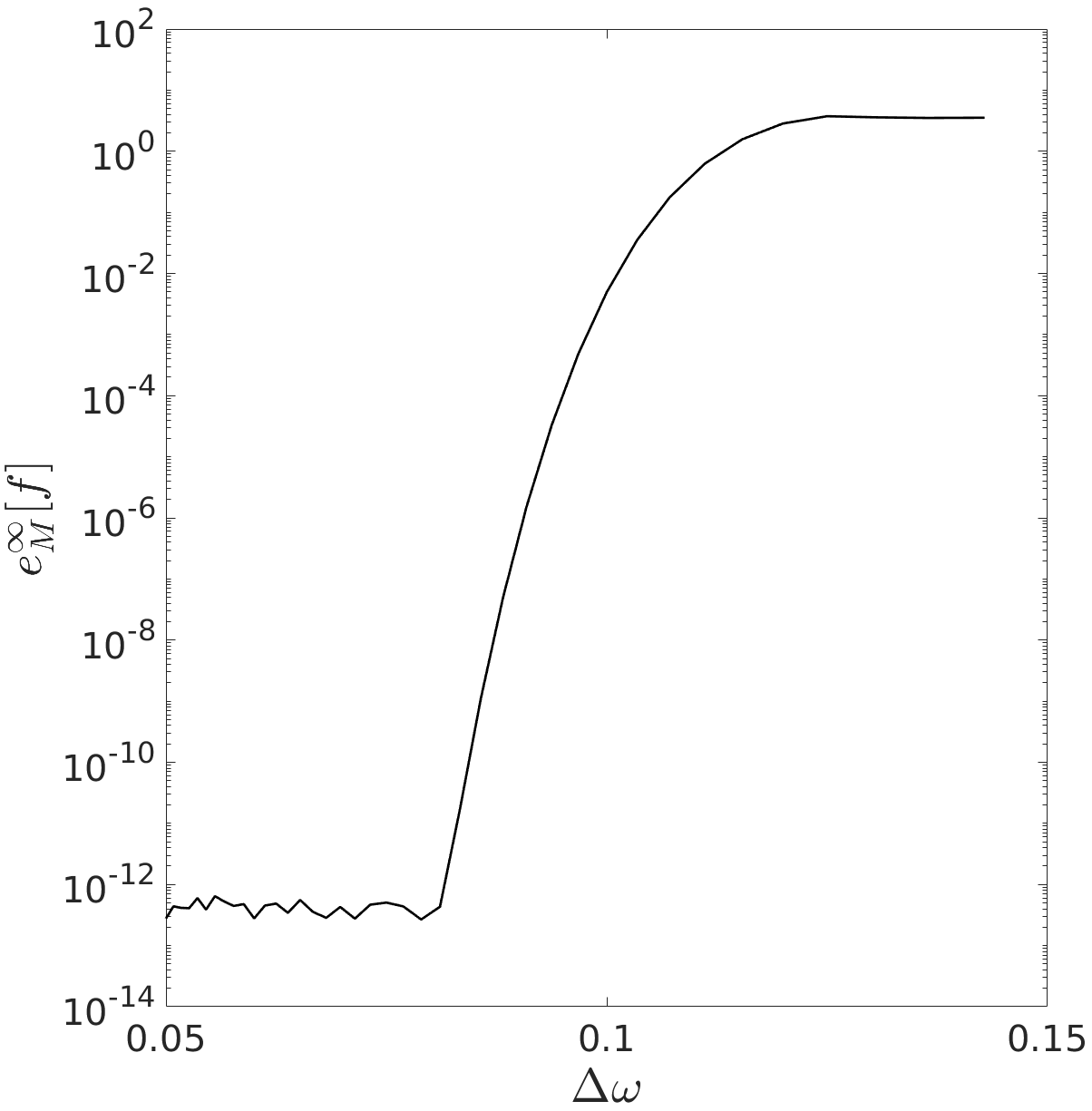
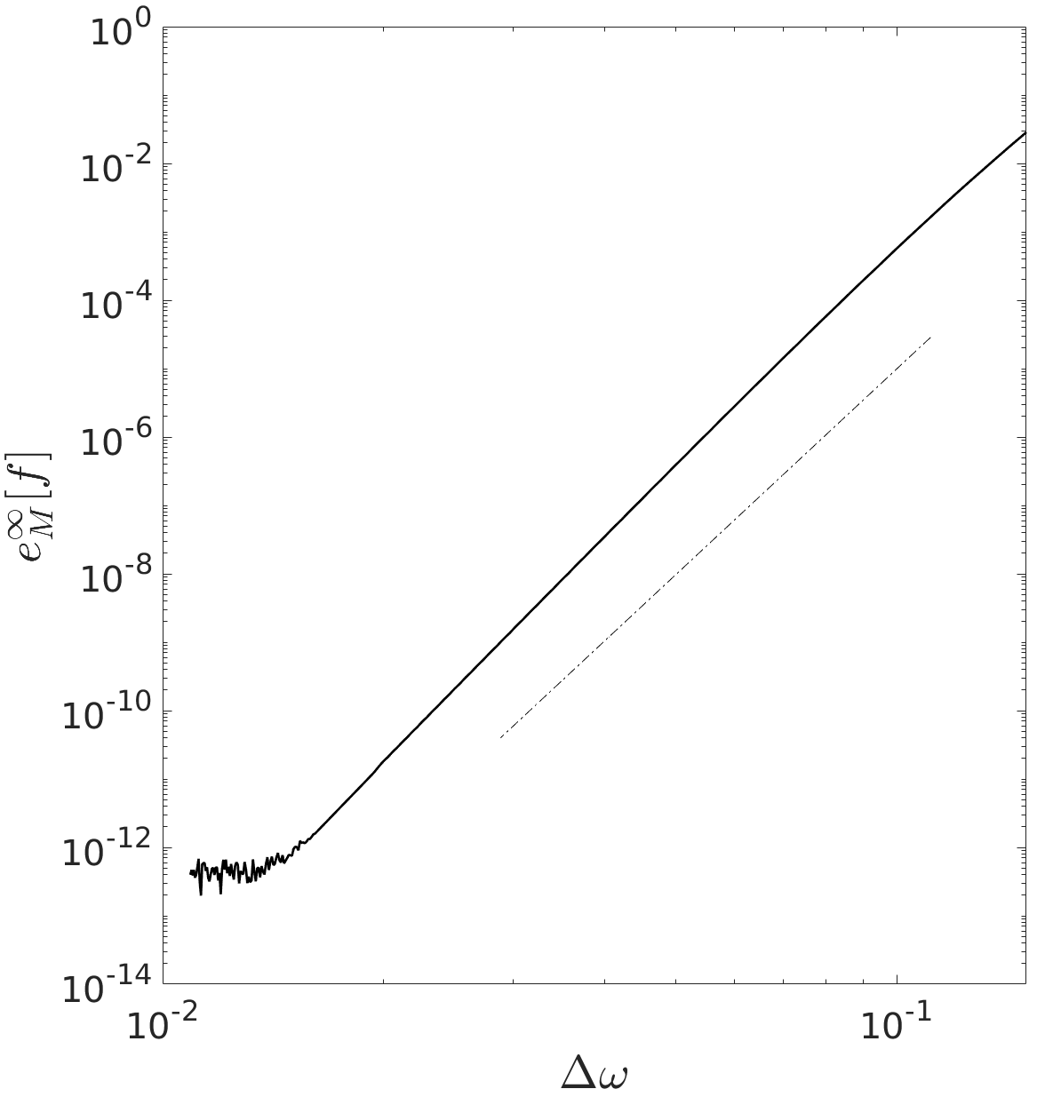
Figure 3: Error $e_{M}^{\infty}$ resulting from the DFT-based (left) and $10\textrm{th}$-order FC(Gram)-based (right) FRFT-accelerated Fourier Transform methods (cf. Remark 9) as a function of $\Delta\omega$. The right figure also includes a $10\textrm{th}$-order slope, for reference.

Figure 3 presents results of an application (to the function $F(\omega)={\mathrm{e}}^{-\frac{1}{4}\omega^{2}}{\mathrm{e}}^{{\mathrm{i}}10\omega}$) of two main components of the Fourier-transform algorithms described in Section 4.1, namely the algorithms that evaluate trigonometric expansions Eq. 32 by means of DFT on one hand, and on the basis of the FC(Gram) algorithm of accuracy order $10$, on the other (cf. Remark 9). (FC expansions of order other than $10$ can of course be used, but order-$10$ expansions were found perfectly satisfactory in our contexts.) Noting that $|F(-12)|=|F(12)|\approx\varepsilon_{\mathrm{mach}}$ (where $\varepsilon_{\mathrm{mach}}$ denotes machine precision), the left (resp. right) portion of Figure 3 displays the accuracy of the Fourier-series based (resp. the FC(Gram)-based) algorithm presented in Section 4.1 for evaluation of Fourier integrals of the form Eq. 30 in interval $[-12,12]$ (resp. in the interval $[0,12]$). The fast (high-order) convergence of the quadrature method as $\Delta\omega\to 0$ that is demonstrated in the present simple example has a significant impact on the efficiency of the algorithm—which requires solution of an expensive integral equation Eq. 10 for each frequency discretization point $\omega_{j}\in\mathcal{F^{\mathrm{smooth}}}$, $\omega_{j+1}-\omega_{j}=\Delta\omega$, for $j=2,\dots,|\mathcal{F}^{\mathrm{smooth}}|=M$ (cf. Remark 10).

6.2 Solution convergence

This section presents solution of a problem of scattering under incident radiation $u^{\textit{inc}}(\mathbf{r},t)$ given by the Fourier transform of the function

(43) $$U^{\textit{inc}}(\mathbf{r},\omega)={\mathrm{e}}^{-\frac{(\omega-\omega_{0})^{2}}{\sigma^{2}}}{\mathrm{e}}^{{\mathrm{i}}\omega\mathbf{\widehat{k}}_{\mathrm{inc}}\cdot\mathbf{r}}$$

with respect to $\omega$, with $\omega_{0}=12$, $\sigma=2$ and, letting $\mathbf{k}=\mathbf{e}_{x}+\frac{1}{2}\mathbf{e}_{y}$, $\mathbf{\widehat{k}}_{\mathrm{inc}}=\frac{\mathbf{k}}{\parallel\mathbf{k}\parallel}$. The scatterer is a two-dimensional kite-shaped structure $(r_{1}(t),r_{2}(t))=(\cos(t)+0.65\cos(2t)-0.65,\allowbreak 1.5\sin(t))$, $(0\leq t\leq 2\pi)$ which is also used in the subsequent example (cf. Fig. 5). Figure 4 presents the time trace of the scattered field displayed in the left image at the observation point $(2,2)$, which lies at a distance of approximately $1.9$ spatial units from the scattering boundary. The right image in Figure 4 displays the error $e$ in the center image as a function of $\Delta\omega$. ( For simplicity, the fixed numerical bandwidth value $W=24$ together with a sufficiently fine fixed spatial discretization were used in all cases to ensure frequency domain solution errors of the order of machine precision.) The right image clearly demonstrates the superalgebraically-fast convergence of the algorithm (relative to a converged reference solution computed with $\Delta\omega=0.12$) as the frequency-domain discretization is refined.

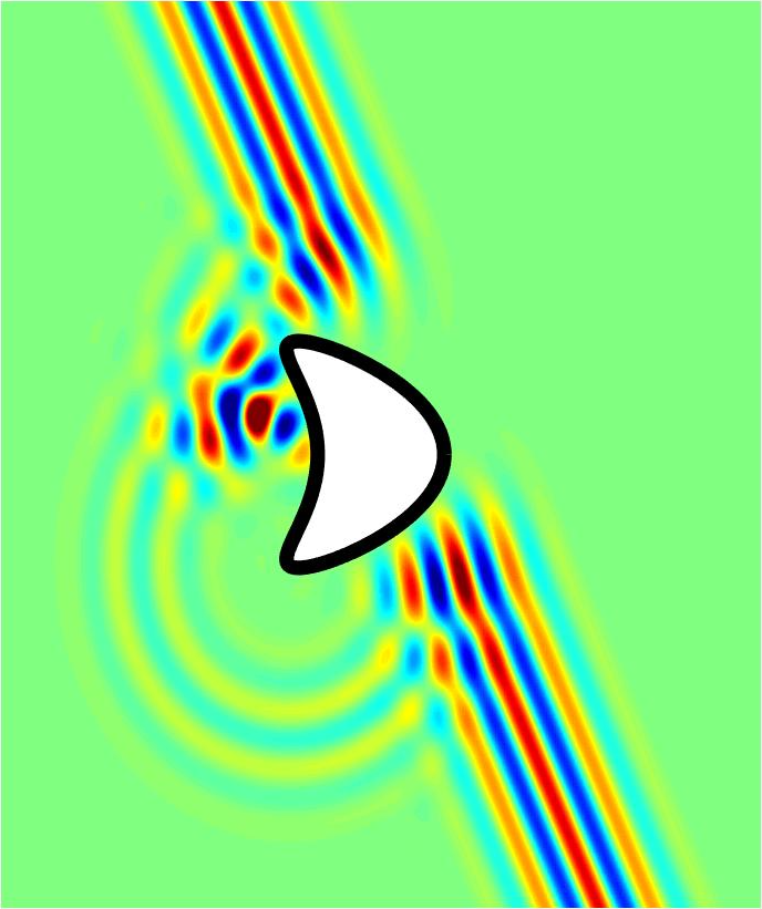
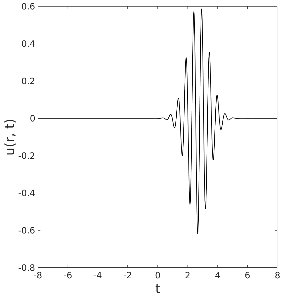
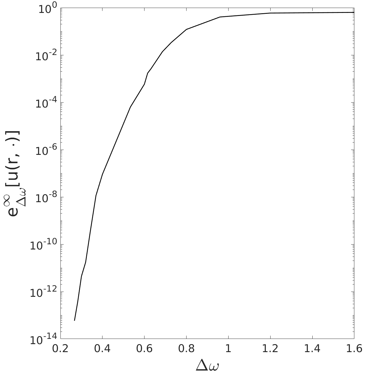
Figure 4: Scattered field (left), time trace at point $\mathbf{r}=(2,2)$ exterior to the scatterer (center) and maximum all-time error $e_{\Delta\omega}^{\infty}$ at $\mathbf{r}=(2,2)$ as a function of the frequency-domain discretization $\Delta\omega$ (right) resulting from an application of the overall fast hybrid method to the problem considered in Section 6.2.

6.3 Full solver demonstration: 2D Examples

This section presents results produced by the proposed methodology for two 2D problems of sound-soft scattering—each of which demonstrates a significant aspect of the proposed approach.

Figure 5: Active-partition tracking demonstration. Each of the four large panels show the solution at increasing times, left to right.

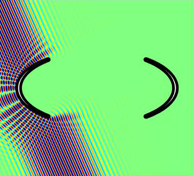
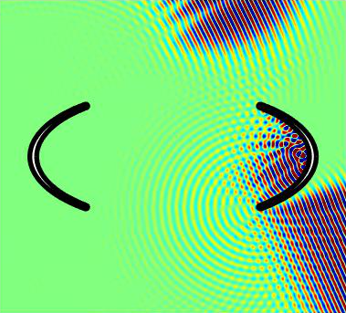
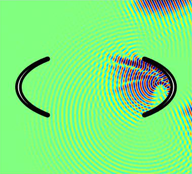
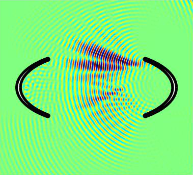
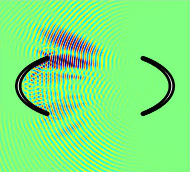
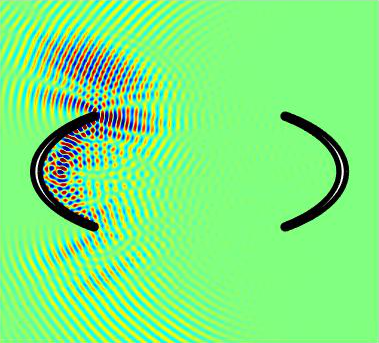
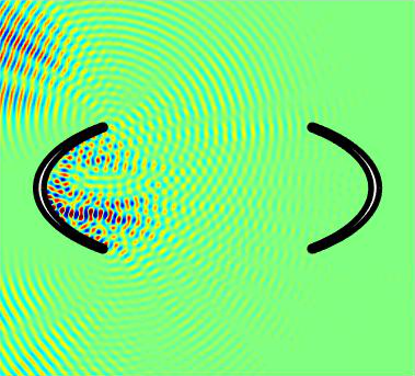
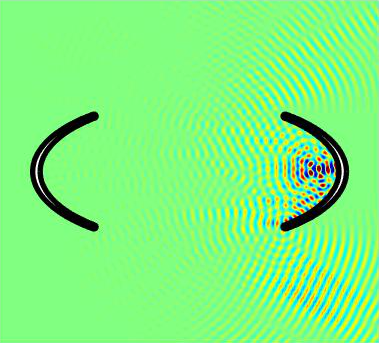
Figure 6: Total fields in the “Whispering Gallery” experiment mentioned in the text. Note the multiple reflections that take place at the elliptical surfaces which, over long propagation times, give rise to a significant number of scattering events. The time sequence starts left-to-right on the first row, and then continues left-to-right on the second row.

Results for incident wave-trains of longer duration which include a time-domain chirp of the form

(44) $$u^{\textit{inc}}(\mathbf{r},t) ={\color[rgb]{0,0,0}-a}(t-\mathbf{r}\cdot\mathbf{\widehat{k}}_{\mathrm{inc}}),\quad\mbox{with}$$

$${\color[rgb]{0,0,0}a}(t) =\sin(g(t)+\frac{1}{4000}g^{2}(t)),$$

$$g(t) =4t+6\cos(\frac{t}{\sqrt{12}}),$$

and $\mathbf{\widehat{k}}_{\mathrm{inc}}$ as in Section 6.2, are presented in Figure 5, which demonstrates the time partitioning strategy Eq. 17 in conjunction with the active partition-tracking method mentioned in Remark 6. The four large panels in this figure display results corresponding to four subsequent time snapshots. In each one of the panels the top-left subfigure presents the total field $u^{\textit{tot}}(\mathbf{r},t)$ at the time represented by the panel. The remaining subfigures in each panel show the contribution to $u^{\textit{tot}}(\mathbf{r},t)$ from each one of the three corresponding time-windowed partitions used in this example. As indicated in Remark 6, blank subfigures in Figure 5 indicate that the corresponding partition does not contribute to $u^{\textit{tot}}$ at the time snapshot represented by the panel. Using an adequate number of time windows (of window width $H=10$) as well as a total of $200$ frequency domain solutions (with bandlimit $W=15$), time domain solutions at any required time can be obtained.

Figure 6 demonstrates the ability of the proposed method to account for complex multiple-scattering effects over long periods of time. The upper left image in this figure displays an incident wave impinging on a “whispering gallery” geometry; subsequent images to the right and in the lower sections of the figure present solution snapshots at a variety of representative times.

6.4 Full solver demonstration: 3D Examples and Comparisons

This section demonstrates the character of the proposed algorithm for 3D problems of sound-soft scattering, and it provides performance comparisons with two solvers introduced recently. All numerical experiments in this section were obtained by means of a Modern Fortran implementation of the proposed approach, using the Intel Fortran compiler version 17.0, on a $24$-core system containing two $12$-core Xeon E$5$-$2670$ CPUs.

Parameter selection, comparison with [12]. $\omega$ $N$ $N_{\beta}$ $N_{\textrm{split}}$ $\varepsilon$ $[5.5,6.5]$ $20$ $150$ $3$ $9.0\cdot 10^{-8}$ $[4.5,5.5]$ $22$ $150$ $2$ $6.7\cdot 10^{-9}$ $[3.5,4.5]$ $21$ $150$ $2$ $1.3\cdot 10^{-8}$ $[2.5,3.5]$ $21$ $130$ $2$ $3.1\cdot 10^{-8}$ $[1.5,2.5]$ $21$ $120$ $2$ $2.7\cdot 10^{-8}$ $[0.0,1.5]$ $20$ $100$ $2$ $5.1\cdot 10^{-8}$

Parameter selection, comparison with [8]. $\omega$ $N$ $N_{\beta}$ $N_{\textrm{split}}$ $\varepsilon$ $[25,45]$ $20$ $90$ $3$ $1.2\cdot 10^{-4}$ $[20,25]$ $18$ $90$ $3$ $1.4\cdot 10^{-4}$ $[10,20]$ $15$ $90$ $3$ $2.8\cdot 10^{-4}$ $[5.0,10]$ $12$ $90$ $2$ $1.8\cdot 10^{-4}$ $[0.0,5.0]$ $10$ $90$ $2$ $1.9\cdot 10^{-5}$

Table 2: Spatial discretizations used for the frequency-domain solver [20] in connection with comparisons with references [12] and [8] and associated numerical errors, for the $\omega$-ranges as listed in the first column of each table. In particular, the tables demonstrate that, as expected, finer discretizations need to be used, for a given desired accuracy, as the acoustical-size of the problems treated grows. In these tables, $N^{2}$ and $N_{\textrm{split}}^{2}$ denote the number of points per patch and the number of patch subdivisions of the original $6$-patch geometry used, respectively, so that the total number of degrees of freedom is $6N^{2}N_{\textrm{split}}^{2}$. (For the definition and significance of the parameter $N_{\beta}$, see [20].) The quantity $\varepsilon$, finally, equals the numerical error at the spatial point $\mathbf{r}=\mathbf{r}_{0}$ with $\mathbf{r}_{0}$ as indicated in the text in each comparison case, for the solution at frequency equal to the upper limit of the frequency interval. Mie series solutions were used in all cases as references for determination of the solution errors $\varepsilon$.

The first example concerns a problem of scattering by a sphere of physical radius $1.6$ (whose choice facilitates certain comparisons) illuminated under plane-wave incidence given by $u^{\textit{inc}}(\mathbf{r},t)={\color[rgb]{0,0,0}-a}(t-\widehat{\mathbf{k}}\cdot\mathbf{r})$, where the signal function $T$ is given by ${\color[rgb]{0,0,0}a}(t)=5e^{-(t-6)^{2}/2}$. The frequency domain was truncated to the interval $[-W,W]$ with numerical bandwidth $W=6.5$, and the problem was then discretized with respect to frequency on the basis of $41$ ( $J=80$) equi-spaced frequencies $\omega$ in the interval $[0,W]$. Approximate solutions to the integral equation Eq. 10 for each one of these frequencies were obtained by means of the linear system solver GMRES with a relative residual tolerance of $10^{-8}$. Table 2 (left) lists the frequency domain spatial discretization parameters used. The row labeled “This work” in Table 4 presents the maximum solution error resulting from an application of the proposed solver together with the corresponding walltime and memory usage. We see that a computing time of approximately four minutes and a memory allocation of 1.2 GB suffice to produce the solution with an absolute maximum error (measured relative to an exact solution obtained via a Mie series representation) of the order of $10^{-7}$ at the observation point $\mathbf{r}=(-1.8,0,0)$, or $0.2$ units away from the scatterer.

—	$||e||_{\infty}$	Time	Mem.
This work	$1.6\cdot 10^{-7}$	$4.1$	$1.2$
Ref. [12]	$\approx 10^{-7}$	$101.75$	$290$

Table 3: Comparison with results in [12]. “This work” data correponds to runs on a $24$-core computer with Sandy Bridge microarchitecture, while reference [12] reports use of a $28$-core computer with the more recent Broadwell microarchitecture. The columns “Time” and “Mem.” list the required wall times (in minutes) and the memory usage (in GB).

—	$||e||_{\infty}$	Time	Mem.
This work	$2.2\cdot 10^{-4}$	$4.3$	$1.6$
Ref. [8]	$2.1\cdot 10^{-3}$	$40.1$	$56.8$

Table 4: Comparison with results in [8]. As in that reference the computational times are reported in CPU core-hours. The columns “Time” and “Mem.” list the required CPU core-hours and the memory usage (in GB). The results in [8] (accelerated) correspond to runs on Santa Rosa Opteron CPUs while the results in “This work” (unaccelerated) were obtained on the more recent Intel Sandy Bridge CPUs.

This example can be related to a test case considered in [12], which introduces a temporally and spatially high-order time-domain integral equation solver, implemented in Matlab, which relies on the built-in sparse matrix-vector multiplication function for time-stepping and a precompiled Fortran function for assembly of the system matrix. A scattering configuration including a physically realizable incident field is considered in [12, Sec. 4.3] which presents computing times but which reports errors in the median. For comparison purposes, however, it seems more appropriate to quantify errors in some adequate norm—and, thus, we chose to provide a comparison with results presented in Sec. 4.2 of that paper—where a “cruller” scattering surface of diameter $3.2$ is used, which is illuminated by an artificial (not physically realizable but commonly used as a test case) point source emanating from a point interior to the surface. In lieu of solving for the specialized cruller geometry, we compare those results to the sphere results provided above. Noting that, with the same diameter, the sphere has a larger surface area ($32.2$ square units) than the cruller geometry ($23.5$ square units), the sphere problem may be considered to be a somewhat more challenging test case in regard to memory usage and computing cost. Errors for the test case in [12, Sec. 4.2] can be read from the second contour plot provided for the cruller geometry in [12, Fig. 8], which displays an error of approximately $10^{-7}$ for $h=\Delta t\approx 0.0367$. The memory usage and computing time required by that test can be deduced from [12, Sec. 4.3], and they amount to $290$ GB of memory and $101.75$ minutes of computing time. (The $101.75=23+\frac{30}{8}\times 21$ minute computing time estimate was obtained as the sum of precomputation and time-stepping times, as reported in [12, Sec. 4.3], but accounting for a simulation over 30 time units, instead of the 8 time units reported in that section.) In view of Table 4 we suggest that, even for short propagation times, the proposed method compares very favorably with the approach [12] in terms of both computational time and memory requirements.

The next example in this section concerns the scattering of a wide-band signal of the form $u^{\textit{inc}}(\mathbf{r},t)=-0.33\sum_{i=1}^{3}\exp\left[\frac{(t-\mathbf{e}_{i}\cdot\mathbf{r}-6\,\sigma-1)^{2}}{\sigma^{2}}\right]$ from the unit sphere, where we have set $\mathbf{e}_{1}=(1,0,0)$, $\mathbf{e}_{2}=(0,1,0)$, $\mathbf{e}_{3}=(0,0,1)$, and $\sigma=0.1$. We solve this problem to an absolute error level of $2.2\cdot 10^{-4}$ (evaluated by comparison with the exact solution obtained via a multi-incidence Mie series representation) at the observation point $\mathbf{r}=\mathbf{r}_{0}=(2.5,0,0)$. The frequency domain was truncated to the interval $[-W,W]$ with numerical bandwidth $W=45$, and the problem was then discretized with respect to frequency on the basis of $91$ ($J=180$) equi-spaced frequencies $\omega$ in the interval $[0,W]$. Approximate solutions to the integral equation Eq. 10 for each one of these frequencies were obtained by means of the linear system solver GMRES with a relative residual tolerance of $10^{-4}$. Table 2 (right) lists the frequency domain spatial discretization parameters used. Figure 7 displays a time-trace of our solution and Table 4 presents relevant performance indicators; the core time listed for our solver was calculated as 24 times the wall time required by the parallelized frequency-domain solver to solve all 91 frequency-domain problems in the 24-core system used, followed by a single core run that evaluates the time trace. Each frequency domain problem was run, in parallel, on all 24 cores.

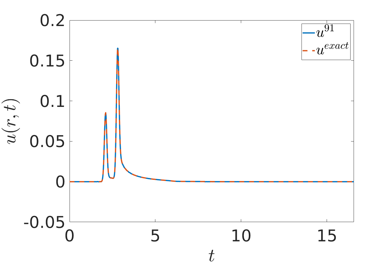
Figure 7: Scattering of a wide-band signal from the unit sphere. This figure presents the time traces of the exact and numerical scattered field computed (on the basis of 91 frequency-domain solutions) by the proposed hybrid method. Corresponding results produced by a novel convolution-quadrature implementation can be found in [8, Figure 5].

This wide-band sphere-scattering example was previously considered in the most recent high-performance implementation [8], including fast multipole and $\mathcal{H}$-matrix acceleration, of the convolution quadrature method. The accuracies produced and the computational costs required by both the present solver (for which frequency-domain solutions were computed without use of acceleration methods) and the one introduced in [8] are presented in Table 4, including CPU core-hours and memory storage. We see that, even without the significant benefits that would arise from frequency-domain operator acceleration in the present context, the proposed solver requires significantly shorter computing times and lower memory allocations, by factors of approximately ten and thirty-five, respectively, when compared with those required by the solver [8]. (Note: the contribution [8] does not directly report the solution error, but it does provide graphical evidence by comparing the time-traces of the solutions obtained, at the observation point $\mathbf{r}=\mathbf{r}_{0}=(2.5,0,0)$, by means of two different spatio-temporal discretizations, for which it was reported that “on this scale [the scale of the graph] the solutions are practically indistinguishable”. A direct comparison of the dataset values (which was kindly provided to us by the authors [40]) to the exact Mie solution allowed us to determine a maximum error of $2.1\cdot 10^{-3}$ in the wide-band sphere test in [8]. Our solution is also graphically indistinguishable from the time-domain response calculated by means of a Mie series, and we report a numerical-solution error of $2.2\cdot 10^{-4}$.)

Finally, Figure 8 presents results of an application of the proposed algorithm to a 3D scatterer (represented by the multi-patch CAD description displayed in the figure), for the Gaussian-modulated incident field

$$U^{\textit{inc}}(\mathbf{r},\omega)={\mathrm{e}}^{-\frac{(\omega-\omega_{0})^{2}}{\sigma^{2}}}{\mathrm{e}}^{{\mathrm{i}}\omega\mathbf{\widehat{k}}_{\mathrm{inc}}\cdot\mathbf{r}}$$

with $\omega_{0}=15$, $\sigma=2$ and $\mathbf{\widehat{k}}_{\mathrm{inc}}=\mathbf{e}_{z}$. (This figure was prepared using the VisIt visualization tool [26].) A total of $250$ frequency domain integral-equation solutions of Equation 10 for frequencies below the numerical bandlimit $W=25$, which were produced by the methodology and software described in [20], suffice to produce the solution for all times.

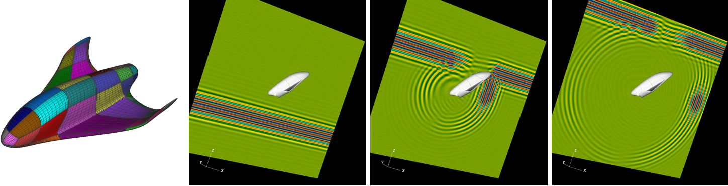
Figure 8: Field scattered by a 3D glider structure.

7 Conclusions

This paper presents the first efficient algorithm for evaluation of time-domain solutions, in two- and three-dimensional space, on the basis of Fourier transformation of frequency domain solutions. The algorithm enjoys superalgebraically fast spectral convergence in both space and time, it runs in $\mathcal{O}(N_{t})$ operations for evaluation of the solution at $N_{t}$ points in time, and it can produce arbitrarily-large time evaluation of scattered fields at $\mathcal{O}(1)$ cost. The method is additionally embarrassingly parallelizable in time and space, and it is amenable to implementations involving a variety of acceleration techniques based on high performance computing.

Appendix A General boundary data: cost estimates and comparisons

As indicated in Remark 1, this appendix briefly discusses possible extensions of the proposed hybrid method that enable solution of problem Eq. 1 for arbitrary incidence-field functions $b(\mathbf{r},t)$ on the basis of a fixed finite set of precomputed frequency-domain solutions that can be obtained in a reasonable computing time. As suggested by that remark the approach could proceed via expansion of a given incident field in source- or scatterer-centered spherical-harmonic expansions; or scattering-boundary-based synthesis relying on principal-component analysis, etc. (For reference, note that, letting the maximum frequency and scatterer’s physical size be denoted by $W$ and $a$, respectively, so that $W\cdot a$ equals the acoustical size of the scatterer at the maximum frequency, $\mathcal{D}=\mathcal{O}((Wa)^{d-1})$ ($d=2$, $3$) denotes the number of frequency domain solutions required [31] by the general-incidence hybrid method at the highest frequency—which is also a bound on the number of frequency domain solutions required, per frequency, for each relevant frequency.) The resulting general-incidence method should prove advantageous. Discretization methods based on time-stepping may be more efficient than the hybrid method for small propagation times, since they do not require precomputations. However, the asymptotic cost estimates presented in what follows and the benefits arising from frequency-domain integral-equation acceleration, as opposed to the more complex time-domain integral-equation acceleration, indicate that significant advantages may result, even in the general incidence case, for scattering problems for which waves traverse the computational domain at least once. Of course the advantages of the hybrid method are much more significant in the most commonly considered single-incidence case—which requires a much more limited set of precomputed frequency-domain solutions. An efficient implementation of the proposed hybrid method for general right-hand sides requires use of frequency-domain solvers which can rapidly produce multiple-incidence solutions, for each given frequency, on the basis of some precomputed direct matrix inverse or LU factorization, etc. For sufficiently small problems a direct LU factorization can be used for this purpose, while, for large problems, fast direct solvers [19, 17, 35, 23, 51] could be utilized: after a generally-significant setup cost, the latter methods can produce, for each relevant frequency, all solutions required by the proposed hybrid method at minimal additional cost. To estimate the costs inherent in the use of fast direct methods in the context of the hybrid solver under general incidence, restricting attention to surface scattering problems considered in this paper, and letting $\mathcal{\widetilde{O}}(X)=\mathcal{O}(X\log(X))$, the $\mathcal{H}$-matrix setup cost for each one of the $\mathcal{O}(Wa)$ required frequencies is a quantity of the order of $\mathcal{\widetilde{O}}((Wa)^{d-1})$. Consideration of numerical experiments presented in [18, Tables 7 & 8] and [19, Table 6] suggest that, if computed by means of a $\mathcal{H}$-matrix approach, the cost to obtain all $\mathcal{D}$ frequency-domain solutions required by the hybrid method, for a given frequency, is itself a quantity of order $\mathcal{\widetilde{O}}((Wa)^{d-1})$. Thus, the cost required for the evaluation of all necessary frequency domain solutions for all $\mathcal{O}(Wa)$ frequencies may be estimated as a quantity of the order of $\mathcal{\widetilde{O}}((Wa)^{d})$. Volumetric time stepping methods (based, say, on finite-differences or finite-elements) over a domain of acoustical size $Wa$, on the other hand, require at least a spatio-temporal discretization, and thus a computing cost, of order $\mathcal{O}((Wa)^{d+1})$ (for simulations long enough that a single crest can traverse the complete computational domain) if a fixed number of points per wavelength are used. Even larger discretizations would be required, in addition, if dispersion is compensated for by decreasing the time-step $\Delta t$ faster than the frequency grows. In any case, a clearly higher operation count results for volumetric solvers than the one presented above for the hybrid method with $\mathcal{H}$-matrix frequency-domain precomputation. If appropriately-accelerated time-domain integral equations are used instead [12, 38, 6], finally, a cost of $\mathcal{\widetilde{O}}((Wa)^{d})$ would result that is asymptotically comparable to the fast-hybrid/direct-solver approach described above—and the relative advantages would depend on other specific characteristics of the methods used, including, in particular, accuracy order and dispersion in time, as well as the quality of the respective acceleration methods used. A comparison of the unaccelerated hybrid method to a recent unaccelerated time-domain integral equation solver is presented in Section 6.4. For most problems arising in applications, however, the incident fields can be represented by a small number of sources, and, in such cases an accelerated version of the hybrid method proposed in this paper already provides clear significant advantages, including improved cost asymptotics, over other methodologies considered in this section.

References

- [1] F. Amlani and O. P. Bruno, An FC-based spectral solver for elastodynamic problems in general three-dimensional domains, Journal of Computational Physics, 307 (2016), pp. 333–354, https://doi.org/10.1016/j.jcp.2015.11.060.
- [2] K. E. Atkinson, The Numerical Solution of Integral Equations of the Second Kind (Cambridge Monographs on Applied and Computational Mathematics), Cambridge University Press, 2009.
- [3] I. M. Babuška and S. A. Sauter, Is the pollution effect of the FEM avoidable for the helmholtz equation considering high wave numbers?, SIAM Journal on Numerical Analysis, 34 (1997), pp. 2392–2423, https://doi.org/10.1137/s0036142994269186.
- [4] D. H. Bailey and P. N. Swarztrauber, The fractional fourier transform and applications, SIAM Review, 33 (1991), pp. 389–404, https://doi.org/10.1137/1033097.
- [5] D. H. Bailey and P. N. Swarztrauber, A fast method for the numerical evaluation of continuous fourier and laplace transforms, SIAM Journal on Scientific Computing, 15 (1994), pp. 1105–1110, https://doi.org/10.1137/0915067.
- [6] A. Bamberger, T. H. Duong, and J. C. Nedelec, Formulation variationnelle espace-temps pour le calcul par potentiel retardé de la diffraction d'une onde acoustique (i), Mathematical Methods in the Applied Sciences, 8 (1986), pp. 405–435, https://doi.org/10.1002/mma.1670080127.
- [7] L. Banjai, Multistep and multistage convolution quadrature for the wave equation: Algorithms and experiments, SIAM Journal on Scientific Computing, 32 (2010), pp. 2964–2994, https://doi.org/10.1137/090775981.
- [8] L. Banjai and M. Kachanovska, Fast convolution quadrature for the wave equation in three dimensions, Journal of Computational Physics, 279 (2014), pp. 103 – 126, https://doi.org/10.1016/j.jcp.2014.08.049.
- [9] L. Banjai, C. Lubich, and J. M. Melenk, Runge–kutta convolution quadrature for operators arising in wave propagation, Numerische Mathematik, 119 (2011), pp. 1–20, https://doi.org/10.1007/s00211-011-0378-z.
- [10] L. Banjai and S. Sauter, Rapid solution of the wave equation in unbounded domains, SIAM Journal on Numerical Analysis, 47 (2009), pp. 227–249, https://doi.org/10.1137/070690754.
- [11] L. Banjai and M. Schanz, Wave propagation problems treated with convolution quadrature and bem, in Fast Boundary Element Methods in Engineering and Industrial Applications, U. Langer, M. Schanz, O. Steinbach, and W. L. Wendland, eds., Springer Berlin Heidelberg, Berlin, Heidelberg, 2012, pp. 145–184, https://doi.org/10.1007/978-3-642-25670-7_5.
- [12] A. H. Barnett, L. Greengard, and T. Hagstrom, High-order discretization of a stable time-domain integral equation for 3d acoustic scattering, 2019, https://arxiv.org/abs/arXiv:1904.00076.
- [13] A. Bayliss and E. Turkel, Radiation boundary conditions for wave-like equations, Communications on Pure and Applied Mathematics, 33 (1980), pp. 707–725, https://doi.org/10.1002/cpa.3160330603.
- [14] J.-P. Berenger, A perfectly matched layer for the absorption of electromagnetic waves, Journal of Computational Physics, 114 (1994), pp. 185–200, https://doi.org/10.1006/jcph.1994.1159.
- [15] T. Betcke, N. Salles, and W. Śmigaj, Overresolving in the laplace domain for convolution quadrature methods, SIAM Journal on Scientific Computing, 39 (2017), pp. A188–A213, https://doi.org/10.1137/16m106474x.
- [16] E. Bleszynski, M. Bleszynski, and T. Jaroszewicz, AIM: Adaptive integral method for solving large-scale electromagnetic scattering and radiation problems, Radio Science, 31 (1996), pp. 1225–1251, https://doi.org/10.1029/96RS02504.
- [17] S. Börm and C. Börst, Hybrid matrix compression for high-frequency problems, 2018, https://arxiv.org/abs/arXiv:1809.04384.
- [18] S. Börm, L. Grasedyck, and W. Hackbusch, Introduction to hierarchical matrices with applications, Engineering Analysis with Boundary Elements, 27 (2003), pp. 405–422, https://doi.org/10.1016/s0955-7997(02)00152-2.
- [19] D. Brunner, M. Junge, P. Rapp, M. Bebendorf, and L. Gaul, Comparison of the fast multipole method with hierarchical matrices for the helmholtz-bem, Computer Modeling in Engineering & Sciences(CMES), 58 (2010), pp. 131–160.
- [20] O. P. Bruno and E. Garza, A chebyshev-based rectangular-polar integral solver for scattering by general geometries described by non-overlapping patches, 2018, https://arxiv.org/abs/1807.01813.
- [21] O. P. Bruno and L. A. Kunyansky, A fast, high-order algorithm for the solution of surface scattering problems: Basic implementation, tests, and applications, Journal of Computational Physics, 169 (2001), pp. 80–110, https://doi.org/10.1006/jcph.2001.6714.
- [22] O. P. Bruno and M. Lyon, High-order unconditionally stable FC-AD solvers for general smooth domains i. basic elements, Journal of Computational Physics, 229 (2010), pp. 2009–2033, https://doi.org/10.1016/j.jcp.2009.11.020.
- [23] O. P. Bruno and A. Pandey, Fast, higher-order direct/iterative hybrid solver for scattering by inhomogeneous media – with application to high-frequency and discontinuous refractivity problems, 2019, https://arxiv.org/abs/arXiv:1907.05914.
- [24] S. N. Chandler-Wilde, I. G. Graham, S. Langdon, and E. A. Spence, Numerical-asymptotic boundary integral methods in high-frequency acoustic scattering, Acta Numerica, 21 (2012), p. 89–305, https://doi.org/10.1017/S0962492912000037.
- [25] Q. Chen, P. Monk, X. Wang, and D. Weile, Analysis of convolution quadrature applied to the time-domain electric field integral equation, Communications in Computational Physics, 11 (2012), p. 383–399, https://doi.org/10.4208/cicp.121209.111010s.
- [26] H. Childs, E. Brugger, B. Whitlock, J. Meredith, S. Ahern, D. Pugmire, K. Biagas, M. Miller, C. Harrison, G. H. Weber, H. Krishnan, T. Fogal, A. Sanderson, C. Garth, E. W. Bethel, D. Camp, O. Rübel, M. Durant, J. M. Favre, and P. Navrátil, VisIt: An End-User Tool For Visualizing and Analyzing Very Large Data, in High Performance Visualization–Enabling Extreme-Scale Scientific Insight, Oct 2012, pp. 357–372.
- [27] R. Coifman, V. Rokhlin, and S. Wandzura, The fast multipole method for the wave equation: A pedestrian prescription, IEEE Antennas and Propagation Magazine, 35 (1993), pp. 7–12.
- [28] D. Colton and R. Kress, Integral Equation Methods in Scattering Theory, Society for Industrial and Applied Mathematics, 11 2013, https://doi.org/10.1137/1.9781611973167.
- [29] V. Domínguez, I. G. Graham, and T. Kim, Filon–clenshaw–curtis rules for highly oscillatory integrals with algebraic singularities and stationary points, SIAM Journal on Numerical Analysis, 51 (2013), pp. 1542–1566, https://doi.org/10.1137/120884146.
- [30] J. Douglas, J. E. Santos, D. Sheen, and L. S. Bennethum, Frequency Domain Treatment Of One-Dimensional Scalar Waves, Mathematical Models and Methods in Applied Sciences, 03 (1993), pp. 171–194, https://doi.org/10.1142/s0218202593000102.
- [31] J. Driscoll and D. Healy, Computing fourier transforms and convolutions on the 2-sphere, Advances in Applied Mathematics, 15 (1994), pp. 202–250, https://doi.org/10.1006/aama.1994.1008.
- [32] B. Engquist and A. Majda, Absorbing boundary conditions for the numerical simulation of waves, Mathematics of Computation, 31 (1977), pp. 629–629, https://doi.org/10.1090/s0025-5718-1977-0436612-4.
- [33] C. L. Epstein, L. Greengard, and T. Hagstrom, On the stability of time-domain integral equations for acoustic wave propagation, Discrete and Continuous Dynamical Systems, 36 (2016), pp. 4367–4382, https://doi.org/10.3934/dcds.2016.36.4367.
- [34] L. N. Frazer and J. F. Gettrust, On a generalization of Filon's method and the computation of the oscillatory integrals of seismology, Geophysical Journal International, 76 (1984), pp. 461–481, https://doi.org/10.1111/j.1365-246x.1984.tb05056.x.
- [35] A. Gillman, A. H. Barnett, and P.-G. Martinsson, A spectrally accurate direct solution technique for frequency-domain scattering problems with variable media, BIT Numerical Mathematics, 55 (2015), pp. 141–170.
- [36] J. Griffith and M. Nakhla, Time-domain analysis of lossy coupled transmission lines, IEEE Transactions on Microwave Theory and Techniques, 38 (1990), pp. 1480–1487, https://doi.org/10.1109/22.58689.
- [37] K. Gröchenig, Foundations of Time-Frequency Analysis, Birkhäuser Boston, 2001, https://doi.org/10.1007/978-1-4612-0003-1.
- [38] T. Ha-Duong, On retarded potential boundary integral equations and their discretisation, in Topics in Computational Wave Propagation: Direct and Inverse Problems, M. Ainsworth, P. Davies, D. Duncan, B. Rynne, and P. Martin, eds., Springer Berlin Heidelberg, Berlin, Heidelberg, 2003, pp. 301–336, https://doi.org/10.1007/978-3-642-55483-4_8.
- [39] T. Hagstrom and T. Warburton, Complete radiation boundary conditions: minimizing the long time error growth of local methods, SIAM J. Numer. Anal., 47 (2009), pp. 3678–3704.
- [40] M. Kachanovska. private communication, ENSTA ParisTech-INRIA-CNRS, France. 04 September 2019.
- [41] R. Kress, On the limiting behaviour of solutions to boundary integral equations associated with time harmonic wave equations for small frequencies, Mathematical Methods in the Applied Sciences, 1 (1979), pp. 89–100, https://doi.org/10.1002/mma.1670010108.
- [42] I. Labarca, L. M. Faria, and C. Pérez-Arancibia, Convolution quadrature methods for time-domain scattering from unbounded penetrable interfaces, Proceedings of the Royal Society A: Mathematical, Physical and Engineering Sciences, 475 (2019), p. 20190029, https://doi.org/10.1098/rspa.2019.0029.
- [43] J.-F. Lee, R. Lee, and A. Cangellaris, Time-domain finite-element methods, IEEE Transactions on Antennas and Propagation, 45 (1997), pp. 430–442, https://doi.org/10.1109/8.558658.
- [44] S. Lin and E. Kuh, Transient simulation of lossy interconnects based on the recursive convolution formulation, IEEE Transactions on Circuits and Systems I: Fundamental Theory and Applications, 39 (1992), pp. 879–892, https://doi.org/10.1109/81.199887, https://doi.org/10.1109/81.199887.
- [45] C. Lubich, On the multistep time discretization of linear initial-boundary value problems and their boundary integral equations, Numerische Mathematik, 67 (1994), pp. 365–389, https://doi.org/10.1007/s002110050033.
- [46] R. C. MacCamy, Low frequency acoustic oscillations, Quarterly of Applied Mathematics, 23 (1965), pp. 247–255, http://www.jstor.org/stable/43635524.
- [47] E. Mecocci, L. Misici, M. C. Recchioni, and F. Zirilli, A new formalism for time-dependent wave scattering from a bounded obstacle, The Journal of the Acoustical Society of America, 107 (2000), pp. 1825–1840, https://doi.org/10.1121/1.428462.
- [48] C. S. Morawetz, Decay for solutions of the exterior problem for the wave equation, Communications on Pure and Applied Mathematics, 28 (1975), pp. 229–264.
- [49] C. S. Morawetz, J. V. Ralston, and W. A. Strauss, Decay of solutions of the wave equation outside nontrapping obstacles, Communications on Pure and Applied Mathematics, 30 (1977), pp. 447–508.
- [50] V. Nascov and P. C. Logofătu, Fast computation algorithm for the rayleigh-sommerfeld diffraction formula using a type of scaled convolution, Appl. Opt., 48 (2009), pp. 4310–4319, https://doi.org/10.1364/AO.48.004310.
- [51] M. Pedneault, C. Turc, and Y. Boubendir, Schur complement domain decomposition methods for the solution of multiple scattering problems, IMA Journal of Applied Mathematics, 82 (2017), pp. 1104–1134.
- [52] S. Petropavlovsky, S. Tsynkov, and E. Turkel, A method of boundary equations for unsteady hyperbolic problems in 3d, Journal of Computational Physics, 365 (2018), pp. 294–323, https://doi.org/10.1016/j.jcp.2018.03.039.
- [53] F.-J. Sayas, Retarded Potentials and Time Domain Boundary Integral Equations, Springer International Publishing, 2016, https://doi.org/10.1007/978-3-319-26645-9.
- [54] I. H. Sloan and W. E. Smith, Product integration with the clenshaw-curtis points: Implementation and error estimates, Numerische Mathematik, 34 (1980), pp. 387–401, https://doi.org/10.1007/bf01403676.
- [55] A. Taflove, Computational electrodynamics : the finite-difference time-domain method, Artech House, Boston, 2000.
- [56] P. Werner, Randwertprobleme der mathematischen akustik, Archive for Rational Mechanics and Analysis, 10 (1962), pp. 29–66.
- [57] P. Werner, Low frequency asymptotics for the reduced wave equation in two-dimensional exterior spaces, Mathematical Methods in the Applied Sciences, 8 (1986), pp. 134–156, https://doi.org/10.1002/mma.1670080110.
- [58] A. Yilmaz, J.-M. Jin, and E. Michielssen, Time domain adaptive integral method for surface integral equations, IEEE Transactions on Antennas and Propagation, 52 (2004), pp. 2692–2708, https://doi.org/10.1109/tap.2004.834399.