Anomalous quartic gauge couplings and unitarization for the vector boson scattering process $pp\rightarrow W^{+}W^{+}jjX\rightarrow\ell^{+}\nu_{\ell}\ell^{+}\nu_{\ell}jjX$

ABSTRACT

Weak vector boson scattering (VBS) at the LHC provides an excellent source of information on the structure of quartic gauge couplings and possible effects of physics beyond the SM in electroweak symmetry breaking. Parameterizing deviations from the SM within an effective field theory at tree level, the dimension-8 operators, which are needed for sufficiently general modeling, lead to unphysical enhancements of cross sections within the accessible energy range of the LHC. Preservation of unitarity limits is needed for phenomenological studies of the $VVjj$ events which signify VBS. Here we develop a numerical unitarization scheme for the full off-shell VBS processes and apply it to same-sign $W$ scattering, i.e. processes like $qq\to qqW^{+}W^{+}$. The scheme is implemented within the Monte Carlo program VBFNLO, including leptonic decay of the weak bosons and NLO QCD corrections. Distributions differentiating between higher dimensional operators are discussed.

1 Introduction

Among the scattering processes which can be studied at the CERN Large Hadron Collider (LHC), weak vector boson scattering (VBS) is particularly interesting as a probe of electroweak symmetry breaking. Within the Standard Model (SM), intricate cancellations between Feynman amplitudes involving quartic gauge boson interactions, trilinear gauge boson couplings, and Higgs exchange lead to scattering amplitudes for longitudinally polarized weak bosons which do not grow with energy and which, for a light Higgs boson, respect bounds derived from unitarity. Modifications of the weak boson couplings, among themselves or to the Higgs boson, spoil these cancellations and can lead to sizable cross section increases. For example, reduced weak boson couplings to the light, $m_{h}=125$ GeV Higgs boson and compensation by an additional heavy Higgs in a two-Higgs-doublet model would lead to a cross section increase at high energy, as would a change only in the quartic gauge couplings.

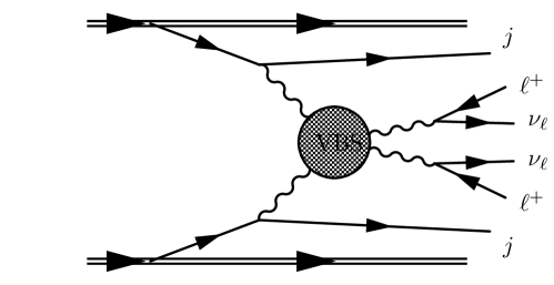
Figure 1: Vector boson scattering contribution to the process $pp\rightarrow W^{+}W^{+}jjX$.

Absent clear hints for a particular theory beyond the Standard Model (BSM), a bottom up approach is conveniently formulated within an effective field theory (EFT) approach [1, 2]. Given the observation of a light Higgs boson at the LHC [3, 4], we opt for a linear representation of the light fields in order to construct dimension-six and -eight operators for the EFT. To give just one example, a deviation in the Higgs sector could manifest itself via the dimension-8 term

$$\mathcal{L}_{S_{1}}=\frac{f_{S_{1}}}{\Lambda^{4}}\left[(D_{\mu}\phi)^{\dagger}D^{\mu}\phi\right]\left[(D_{\nu}\phi)^{\dagger}D^{\nu}\phi\right]\,,$$ (1)

in the effective Lagrangian, which is present in the linear Éboli-basis [5]. Here, the covariant derivative of the Higgs-doublet field, $D^{\mu}\phi$, contains $W$ and $Z$ fields, $\Lambda$, is the energy scale of new physics, and the coupling coefficient $f_{S_{1}}$ is used later to allow different strengths for independent dimension-8 operators. This operator will induce an anomalous contribution to the four-$W$, four-$Z$, and $WWZZ$ vertices, which alter the scattering (predominantly) of the longitudinal degrees of freedom of the weak vector bosons. The impact of anomalous couplings on $VV\to VV$ scattering can be studied at the LHC via the full process $pp\rightarrow VVjjX$ as illustrated in Fig. 1, where the two final state vector bosons $V$ can decay either leptonically or hadronically.

The current, observed limits for ${f_{S_{1}}/\Lambda^{4}}$, derived from same-sign $W$ scattering by CMS, are $\left[-21.6,21.8\right]\;\text{TeV}^{-4}$ for 35.9 fb^-1 of $\sqrt{s}=13\;\text{TeV}$ data [6]. We are not aware of new results for Run-II published by ATLAS. However, comparing old limits for ${f_{S_{1}}/\Lambda^{-4}}$ of $\left[-118,120\right]\;\text{TeV}^{-4}$ from 19.4 fb^-1 of $\sqrt{s}=8\;\text{TeV}$ data from CMS [7] and $\left[-960,960\right]\;\text{TeV}^{-4}$ from 20.3 fb^-1 of $\sqrt{s}=8\;\text{TeV}$ data from ATLAS [8], one observes a substantial difference in precision. This difference is mainly due to the different high-energy extrapolation of the EFT ansatz in the generation of BSM Monte-Carlo events. The EFT is only valid up to a certain energy scale $\Lambda_{\mathrm{valid}}<\Lambda$, where the operator product expansion breaks down. However, the experiment is only sensitive to the ratio ${f_{S_{1}}/\Lambda^{4}}$ and the scale $\Lambda$ is a priori not known. Using just the EFT as input for the generation of Monte Carlo data will usually overshoot any result allowed by perturbative unitarity in the high energy region. Naturally this will result in more stringent limits for the EFT-coefficients. CMS is using this approach in presenting their limits. ATLAS on the other hand is using the T-matrix [12, 13] unitarization scheme to provide a theoretically consistent description of the high energy region, where unitarity would otherwise be violated, with a proper interpolation to the low energy EFT. T-matrix unitarization leads to lower generated event rates for a given ${f_{S_{1}}/\Lambda^{4}}$, which leads to weaker limits for this Wilson coefficient.

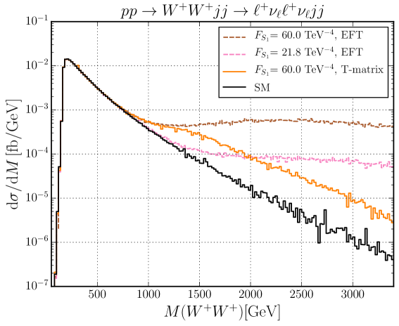
Figure 2: Differential cross section as a function of the invariant mass $m_{VV}$ of the weak vector bosons for $pp\rightarrow\ell^{+}\nu_{\ell}\ell^{+}\nu_{\ell}jjX$. The solid black line represents the SM, while the dashed pink and dashed brown lines show the EFT cross section for the $F_{S1}={f_{S_{1}}/\Lambda^{4}}$ anomalous coupling. The solid orange line shows the T-matrix unitarized curve with the same fiducial cross section as the orange pure EFT curve. Cuts defining the fiducial region are given in Eq. (34).

The effect is demonstrated in Fig. 2, where we compare the $W^{+}W^{+}$ invariant mass distribution expected with the current CMS limit $F_{S_{1}}={f_{S_{1}}/\Lambda^{4}}=21.8$ TeV^-4 for a naive EFT description (dashed pink), with a T-matrix unitarized [12] prescription, with larger coupling $F_{S_{1}}=60$ TeV^-4, which will give the same fiducial cross section (solid orange histogram). Also shown are the SM expectation (solid black) and the naive EFT expectation for the larger coupling of 60 TeV^-4 (dashed brown), which agrees with the T-matrix unitarized expectation only at small invariant masses. In the energy range above $M_{WW}\approx 1500$ GeV, an $\mathcal{L}_{S_{1}}$ induced excess above the orange $F_{S_{1}}=60$ TeV^-4 curve violates unitarity, i.e. it is unphysical, and should therefore not be considered to estimate EFT coefficients. This is quite general: a pure effective Lagrangian/anomalous coupling analysis of LHC observables, with a finite set of terms in the effective Lagrangian, is insufficient in practice because the unbounded growth of amplitudes with energy typically corresponds to unitarity violation within the energy reach of the LHC. We thus need a general and versatile unitarization procedure for the naive EFT amplitudes at high momentum transfers, which smoothly interpolates to the pure EFT description well below $\Lambda_{\mathrm{valid}}$.

In order to analyze $VVjj$ production data, any unitarity considerations for $VV\to VV$ scattering must be extrapolated from on-shell bosons to the space-like incoming and time-like outgoing virtualities of the vector bosons which is implicit in the kinematics of Fig. 1. As we shall see, this extrapolation will require a few additional assumptions and will induce some model dependence. To obtain predictions which are compatible with unitarity, the T-matrix unitarization prescription can be used. So far, however, an implementation of this scheme is only available for a small number of effective Lagrangian operators for VBS due to the difficulty to handle VBS with arbitrarily polarized off-shell vector bosons in the full $VVjj$ production process [12, 13]. In this paper, we introduce a variant of the T/K-matrix unitarization scheme [12, 14], called $T_{u}$ unitarization below, for general combinations of operators within VBS, for arbitrary space-like virtualities of the incoming vector bosons, and describe its implementation in the Monte Carlo generator VBFNLO [15, 16, 17].

The paper is organized as follows. We introduce the full set of bosonic dimension-8 operators with a list of current experimental limits in Section 2. In Section 3, we first consider how unitarity relations can be extended to off-shell VBS processes. Beyond the definition of off-shell polarization vectors, this entails partial wave decomposition for off shell sub-amplitudes for $VV\to VV$ scattering and its fast numerical implementation. The $T_{u}$ unitarization model, which we have implemented in VBFNLO for same-sign $W$ scattering, is introduced in Section 3.3. Section 4 is devoted to numerical results for same-sign $W$-scattering, i.e the process $pp\rightarrow W^{+}W^{+}jjX\rightarrow\ell^{+}\nu_{\ell}\ell^{+}\nu_{\ell}jjX$ at NLO QCD precision, which is now implemented in VBFNLO including $T_{u}$ unitarization for any combination of the dimension-8 operators listed in Section 2. We compare our $T_{u}$ unitarized model with naive EFT descriptions for different dimension-8 operators. Furthermore, we will also give examples of observables helping to distinguish experimentally between different subclasses of dimension-8 operators. Final conclusions are drawn in Section 5.

2 Effective Field Theory Description of
Anomalous Quartic Gauge Couplings

The bottom-up EFT framework is useful to quantify deviations from the SM in a model independent way and, once experimental evidence for such deviations is discovered, it gives hints, from which BSM effect a possible anomaly might originate. Short of such a desirable situation, experimental limits on the Wilson coefficients serve as a measure of the experimental precision. Two EFT representations are mainly used to describe BSM contributions for anomalous quartic gauge couplings, the linear and non-linear representation. They can be distinguished due to the different ordering of the EFT expansion

$$\mathcal{L}_{\mathrm{EFT}} =\sum_{i}\frac{f_{i}}{\Lambda^{d_{i}-4}}\mathcal{O}_{i}\,,$$ (2)

which is written in terms of operators $\mathcal{O}_{i}$ of energy dimension $d_{i}$, corresponding Wilson coefficients $f_{i}$ (which allow for variations in importance of the individual operators) and energy scale of new physics, $\Lambda$. In the non-linear representation, the Higgs couplings are treated as additional free parameters and deviations in the Higgs sector can already be introduced at lowest order [18]. This was well motivated before the experimental Higgs discovery in case of a heavy or strongly interacting Higgs [19, 20]. However, since no deviations from the light SM Higgs predictions have been observed so far, we choose the linear Higgs representation, where deviations from the SM predictions for Higgs couplings and trilinear or quartic gauge boson first appear at energy dimension $d_{i}=6$ [21, 22, 23].

Anomalous quartic gauge couplings (aQGC) are induced at the dimension-6 level already. However, they are not independent of changes in the Higgs couplings or of anomalous trilinear gauge couplings. These three-boson couplings are most easily measured in Higgs production or decay or in vector boson pair production ($q\bar{q}\to V_{1}V_{2}$), at the LHC, and little additional information is to be expected from the measurement of the significantly smaller VBS cross sections. Also, the tensor structure of dimension-6 operators is not general enough to allow for sufficiently uncorrelated variations of the 81 helicity amplitudes which, in principle, can be probed in a VBS process, $V_{1}V_{2}\to V_{3}V_{4}$, with massive vector bosons. In this paper, we study aQGC which enter the EFT at lowest order at dimension-8 without contributing to anomalous trilinear gauge interactions or to $HVV$ couplings.

The contributing CP conserving operators can be assembled from three SM building blocks. One building block is the covariant derivative acting on the Higgs doublet field,

$$D_{\mu}\Phi\equiv\left(\partial_{\mu}+i\frac{g^{\prime}}{2}B_{\mu}+igW_{\mu}^{i}\frac{\tau^{i}}{2}\right)\Phi,$$ (3)

which affects the coupling of longitudinal modes of the gauge bosons. Here, the Higgs, $H$ is embedded in the Higgs doublet field in the unitary gauge:

$$\Phi =\begin{pmatrix}0\\ \frac{v+H}{\sqrt{2}}\end{pmatrix}\,.$$ (4)

The other building blocks are the field strength tensors

$$\widehat{W}_{\mu\nu} =ig\frac{\tau^{i}}{2}(\partial_{\mu}W^{i}_{\nu}-\partial_{\nu}W^{i}_{\mu}-g\epsilon_{ijk}W^{j}_{\mu}W^{k}_{\nu})\,,$$ (5a)

$$\widehat{B}_{\mu\nu} =\frac{i}{2}g^{\prime}(\partial_{\mu}B_{\nu}-\partial_{\nu}B_{\mu})\;,$$ (5b)

which are normalized such that $[D_{\mu},D_{\nu}]=\widehat{W}_{\mu\nu}+\widehat{B}_{\mu\nu}$ for the covariant derivative in Eq. (3). The abelian parts of these field strength tensors lead to couplings of the transverse degrees of freedom of the gauge fields.

The dimension-8 operators are separated into longitudinal, transverse, and mixed contributions, corresponding to the occurrence of the building blocks above. A revised list of dimension-8 operators from [5] and [24] is given in Eqs. (6,7,8). In comparison to the operators defined in [5], we choose a different normalization for the field strength in Eq. (5), which is accompanied by an additional factor of $\mathrm{i}g$ or $\mathrm{i}g^{\prime}/2$. These normalization choices are labeled as ”Éboli” for [5] and the normalization in Eq. (5) as ”VBFNLO”, in the following.

For the longitudinal operators the two normalization choices coincide:

$${\cal O}_{S_{0}} =\left[\left(D_{\mu}\Phi\right)^{\dagger}D_{\nu}\Phi\right] \times\left[\left(D^{\mu}\Phi\right)^{\dagger}D^{\nu}\Phi\right]\,,$$ (6a)

$${\cal O}_{S_{1}} =\left[\left(D_{\mu}\Phi\right)^{\dagger}D^{\mu}\Phi\right] \times\left[\left(D_{\nu}\Phi\right)^{\dagger}D^{\nu}\Phi\right]\,$$ (6b)

$${\cal O}_{S_{2}} =\left[\left(D_{\mu}\Phi\right)^{\dagger}D_{\nu}\Phi\right] \times\left[\left(D^{\nu}\Phi\right)^{\dagger}D^{\mu}\Phi\right]\,.$$ (6c)

Compared to Ref. [5], the longitudinal operator set is extended by the operator $\mathcal{O}_{S_{2}}$, which is needed for a simultaneous matching to the non-linear basis for all weak boson flavor combinations in VBS [11, 24]. The mixed set is given by

$${\cal O}_{M_{0}} =\hbox{Tr}\left[{\widehat{W}}_{\mu\nu}{\widehat{W}}^{\mu\nu}\right]\times\left[\left(D_{\beta}\Phi\right)^{\dagger}D^{\beta}\Phi\right]\,,$$ (7a)

$${\cal O}_{M_{1}} =\hbox{Tr}\left[{\widehat{W}}_{\mu\nu}{\widehat{W}}^{\nu\beta}\right]\times\left[\left(D_{\beta}\Phi\right)^{\dagger}D^{\mu}\Phi\right]\,,$$ (7b)

$${\cal O}_{M_{2}} =\left[{\widehat{B}}_{\mu\nu}{\widehat{B}}^{\mu\nu}\right]\times\left[\left(D_{\beta}\Phi\right)^{\dagger}D^{\beta}\Phi\right]\,,$$ (7c)

$${\cal O}_{M_{3}} =\left[{\widehat{B}}_{\mu\nu}{\widehat{B}}^{\nu\beta}\right]\times\left[\left(D_{\beta}\Phi\right)^{\dagger}D^{\mu}\Phi\right]\,,$$ (7d)

$${\cal O}_{M_{4}} =\left[\left(D_{\mu}\Phi\right)^{\dagger}{\widehat{W}}_{\beta\nu}D^{\mu}\Phi\right]\times{\widehat{B}}^{\beta\nu}\,,$$ (7e)

$${\cal O}_{M_{5}} =\left[\left(D_{\mu}\Phi\right)^{\dagger}{\widehat{W}}_{\beta\nu}D^{\nu}\Phi\right]\times{\widehat{B}}^{\beta\mu}\,,$$ (7f)

$${\cal O}_{M_{5}^{\prime}} =\left[\left(D_{\mu}\Phi\right)^{\dagger}{\widehat{W}}^{\beta\mu}D^{\nu}\Phi\right]\times{\widehat{B}}_{\beta\nu}\,,$$ (7g)

$${\cal O}_{M_{7}} =\left[\left(D_{\mu}\Phi\right)^{\dagger}{\widehat{W}}_{\beta\nu}{\widehat{W}}^{\beta\mu}D^{\nu}\Phi\right]\,.$$ (7h)

The operator ${\mathcal{O}}_{M_{6}}$ of the original operator set in [5] is not independent of the others (${\mathcal{O}}_{M_{0}}=2{\mathcal{O}}_{M_{6}}$) and can therefore be omitted. We have added $\mathcal{O}_{M_{5}^{\prime}}$, which is the hermitian conjugate of $\mathcal{O}_{M_{5}}$, and has to be included to complete the operator set. Finally, the purely transverse operators are

$${\cal O}_{T_{0}} =\hbox{Tr}\left[{\widehat{W}}_{\mu\nu}{\widehat{W}}^{\mu\nu}\right] \times\hbox{Tr}\left[{\widehat{W}}_{\alpha\beta}{\widehat{W}}^{\alpha\beta}\right]\,,$$ (8a)

$${\cal O}_{T_{1}} =\hbox{Tr}\left[{\widehat{W}}_{\alpha\nu}{\widehat{W}}^{\mu\beta}\right] \times\hbox{Tr}\left[{\widehat{W}}_{\mu\beta}{\widehat{W}}^{\alpha\nu}\right]\,,$$ (8b)

$${\cal O}_{T_{2}} =\hbox{Tr}\left[{\widehat{W}}_{\alpha\mu}{\widehat{W}}^{\mu\beta}\right] \times\hbox{Tr}\left[{\widehat{W}}_{\beta\nu}{\widehat{W}}^{\nu\alpha}\right]\,,$$ (8c)

$${\cal O}_{T_{5}} =\hbox{Tr}\left[{\widehat{W}}_{\mu\nu}{\widehat{W}}^{\mu\nu}\right] \times{\widehat{B}}_{\alpha\beta}{\widehat{B}}^{\alpha\beta}\,,$$ (8d)

$${\cal O}_{T_{6}} =\hbox{Tr}\left[{\widehat{W}}_{\alpha\nu}{\widehat{W}}^{\mu\beta}\right] \times{\widehat{B}}_{\mu\beta}{\widehat{B}}^{\alpha\nu}\,,$$ (8e)

$${\cal O}_{T_{7}} =\hbox{Tr}\left[{\widehat{W}}_{\alpha\mu}{\widehat{W}}^{\mu\beta}\right] \times{\widehat{B}}_{\beta\nu}{\widehat{B}}^{\nu\alpha}\,,$$ (8f)

$${\cal O}_{T_{8}} ={\widehat{B}}_{\mu\nu}{\widehat{B}}^{\mu\nu}{\widehat{B}}_{\alpha\beta}{\widehat{B}}^{\alpha\beta} \,,$$ (8g)

$${\cal O}_{T_{9}} ={\widehat{B}}_{\alpha\mu}{\widehat{B}}^{\mu\beta}{\widehat{B}}_{\beta\nu}{\widehat{B}}^{\nu\alpha} \,.$$ (8h)

Same-sign $W$ boson scattering is the VBS process which can be measured with the highest precision, due to a sizable signal cross section and a particularly low QCD background [6, 7, 8]. In Section 4 we will concentrate on this process, to which only operators with exactly four $W^{\pm}$ fields can contribute at tree level. This eliminates all operators with a hypercharge field strength, ${\widehat{B}}_{\mu\nu}$. The remaining ones have been probed by ATLAS [8] and CMS [6, 7] in same-sign $W$ scattering, and the results are summarized in Table 1.

Measurement	CMS, 13 TeV[6]	CMS, 13 TeV	ATLAS, 8 TeV[8]	CMS, 8 TeV[7]
Normalization	Éboli	VBFNLO	VBFNLO (T-matrix)	Éboli
$f_{S_{0}}/\Lambda^{4}$	[-7.7,7.7]	[-7.7,7.7]		[-38,40]
$f_{S_{1}}/\Lambda^{4}$	[-21.6,21.8]	[-21.6,21.8]	[-960,960]	[-118,120]
$f_{M_{0}}/\Lambda^{4}$	[-6.0,5.9]	[-14,15]		[-33,32]
$f_{M_{1}}/\Lambda^{4}$	[-8.7,9.1]	[-22,21]		[-44,47]
$f_{M_{6}}/\Lambda^{4}$	[-11.9,11.8]	[-28.7,28.9]		[-65,63]
$f_{M_{7}}/\Lambda^{4}$	[-13.3,12.9]	[-31.4,32.3]		[-70,66]
$f_{T_{0}}/\Lambda^{4}$	[-0.62,0.65]	[-3.7,3.8]		[-4.2,4.6]
$f_{T_{1}}/\Lambda^{4}$	[-0.28,0.31]	[-1.7,1.8]		[1.9,2.2]
$f_{T_{2}}/\Lambda^{4}$	[-0.89,1.02]	[-5.3,6.0]		[-5.2,6.4]

Table 1: Experimental limits (in TeV^-4) on the coefficients of dimension-8 operators, $f_{i}/\Lambda^{4}$, from observation of $pp~{}\rightarrow~{}W^{\pm}W^{\pm}~{}jjX$.

In comparing the different normalization of Éboli and VBFNLO, one finds that the limits for VBFNLO differ by about one order of magnitude only, whereas the limits in the Éboli normalization vary by up to two orders of magnitude. The difference is simply due to consistently factorizing the small electroweak couplings, which are expected for any model explaining the EFT, into the definition of the operators for the VBFNLO normalization convention. For the 8 TeV data, the ATLAS result incorporates a unitarization model to prevent the generation of unphysical events at high energy, which violate unitarity constraints. The corresponding bound on $f_{S_{1}}/\Lambda^{4}$ for the same-sign W scattering process observed by ATLAS [8] is approximately one order of magnitude weaker than the CMS $\sqrt{s}=8\,\mathrm{TeV}$ limit, which indicates the impact that unitarization can have on quoted experimental results.

3 Unitarity for VBS: going off-shell

We need to apply unitarity considerations to electroweak processes of the type $pp\rightarrow\bar{\psi_{1}}\psi_{2}\bar{\psi_{3}}\psi_{4}jj$ at ${\cal O}(\alpha^{6})$ (LO) and at ${\cal O}(\alpha^{6}\,\alpha_{s})$ (NLO), i.e. including QCD corrections. At the parton level, the $\psi_{i}$ represent decay leptons of two vector bosons, the initial $pp$ state represents the scattering partons (quarks or anti-quarks in the LO case) and $jj$ stands for the final state partons yielding two tagging jets. Representative Feynman graphs for the 8-fermion processes at LO are given in Fig. 3 and include vector boson emissions off quark lines as in Fig. 3a as well as VBS contributions as in Fig. 3b. The BSM physics, which we consider via the introduction of bosonic operators, will only contribute to the VBS subprocess $VV\rightarrow VV$. The SM contributions to the complete process are gauge invariant by themselves, they are “small” and they respect perturbative unitarity. Splitting the full amplitude into the SM and a BSM piece,

$$\mathcal{M}_{pp\rightarrow 4fjj} =\mathcal{M}_{pp\rightarrow 4fjj}^{\rm SM}+\mathcal{M}_{pp\rightarrow 4fjj}^{\rm BSM}\,,$$ (9)

it is, therefore, sufficient to unitarize the BSM piece only, via the VBS subprocess, which means that we neglect the interference of SM and BSM amplitudes for unitarization.

(a) Vector boson emission

(b) Quartic gauge interaction.

Figure 3: Examples of Feynman graphs contributing to vector boson scattering.

3.1 Identification of the $VV\rightarrow VV$ Subamplitude

Within the VBFNLO approach, the entire $VV\rightarrow VV$ subprocess is contained inside a leptonic tensor, which then is contracted with quark currents, $J^{\mu}_{p\rightarrow jV}$. These represent the emission of a virtual vector boson, $V$, off an initial parton in Fig. 3b. This structure is well suited to implement the BSM amplitude as

$$\mathcal{M}_{pp\rightarrow 4fjj}^{\rm BSM} =J^{\mu}_{p_{1}\rightarrow jV_{1}}J^{\nu}_{p_{2}\rightarrow jV_{2}}\,\mathcal{M}_{V_{1}V_{2}\rightarrow 4f\,\mu\nu}^{\rm BSM}\,,$$ (10)

where $\mathcal{M}_{V_{1}V_{2}\rightarrow 4f\,\mu\nu}^{\rm BSM}$ denotes the BSM contribution to the leptonic tensor.

The quark currents, $J^{\mu}_{p\rightarrow jV}$, and the decay currents, $J_{V\rightarrow\bar{f}f}^{\mu}$, are conserved, since we are neglecting fermion masses, and this allows for a simple expansion of the off-shell vector boson propagators in terms of polarization vectors of fixed helicity. When writing

$$\mathcal{M}_{pp\rightarrow 4fjj}^{\rm BSM}= J_{p_{1}\rightarrow jV_{1}}^{\mu}\ J_{p_{2}\rightarrow jV_{2}}^{\nu}\ D_{\mu\alpha}^{V_{1}}(q_{1})\ D_{\nu\beta}^{V_{2}}(q_{2})$$

$$\times\textnormal{\bf M}_{V_{1}V_{2}\rightarrow V_{3}V_{4}}^{\alpha\beta\gamma\delta}\ D_{\gamma\rho}^{V_{3}}(q_{3})\ D_{\delta\sigma}^{V_{4}}(q_{4})$$ (11)

$$\times J_{V_{3}\rightarrow\bar{f}f}^{\rho}\ J_{V_{4}\rightarrow\bar{f}f}^{\sigma}\,,$$

the vector boson propagators may be taken as

$$D^{\mu\nu}_{V}(q)=\frac{-\mathrm{i}}{q^{2}-m_{V}^{2}+i\,m_{V}\,\Gamma_{V}}\left(g^{\mu\nu}-\frac{q^{\mu}q^{\nu}}{q^{2}}\right)\equiv\frac{-\mathrm{i}}{q^{2}-m_{V}^{2}+i\,m_{V}\,\Gamma_{V}}\sum_{\lambda}\epsilon_{J}^{*\,\mu}(q,\lambda){\epsilon}_{\mathcal{M}}^{\nu}(q,\lambda)\,$$ (12)

since the $q^{\mu}$ terms are contracted with a conserved current and, thus, vanish. The indices $J$ and $\mathcal{M}$ on the polarization vectors distinguish between those that are contracted with the currents, $\epsilon_{J}$, and the polarization vectors contracted with the VBS matrix element, $\epsilon_{\mathcal{M}}$. Furthermore, we generalize the definition of the polarization vectors for off-shell vector bosons with four-momentum $q$ to

$$\epsilon^{\mu}_{J}(q,\pm) =\mp\frac{1}{\sqrt{2}\sqrt{q_{x}^{2}+q_{y}^{2}}}\left(0;\frac{q_{z}q_{x}}{|\vec{q}|}\mp\mathrm{i}q_{y},\frac{q_{y}q_{z}}{|\vec{q}|}\pm\mathrm{i}q_{x},-\frac{q_{x}^{2}+q_{y}^{2}}{|\vec{q}|}\right)=\epsilon^{\mu}_{\mathcal{M}}(q,\pm)\,,$$ (13a)

$$\epsilon^{\mu}_{J}(q,0) =\mathcal{N}_{J}\left(|\vec{q}|,\,q_{0}\frac{\vec{q}}{|\vec{q}|}\right)\,,\qquad\qquad\qquad\qquad\mathcal{N}_{\mathcal{M}}\left(|\vec{q}|,\,q_{0}\frac{\vec{q}}{|\vec{q}|}\right)=\epsilon^{\mu}_{\mathcal{M}}(q,0)\,,$$ (13b)

where $\mathcal{N}_{\mathcal{M}}$ and $\mathcal{N}_{J}$ have to fulfill $\mathcal{N}_{J}\mathcal{N}_{\mathcal{M}}=1/q^{2}$ as normalization factors for the longitudinal polarization vectors. One could choose the individual factors to be equal in magnitude. However, in order to match the proper normalization for on-shell weak bosons and thus to reproduce the correct normalization of $VV\rightarrow VV$ scattering amplitudes for longitudinal $V$, we set

$$\mathcal{N}_{J}=\frac{m_{V}}{q^{2}}\,,\qquad\mathcal{N}_{\mathcal{M}}=\frac{1}{m_{V}}.$$ (14)

With these definitions, the BSM contribution to the leptonic tensor becomes

$$\mathcal{M}_{V_{1}V_{2}\rightarrow 4f,\mu\nu}^{\rm BSM}= \prod_{i=1}^{4}\frac{1}{q_{i}^{2}-m_{V_{i}}^{2}+i\,m_{V_{i}}\,\Gamma_{V_{i}}}\sum_{\{\lambda_{i}\}}\epsilon^{*}_{J,\mu}(q_{1},\lambda_{1})\epsilon^{*}_{J,\nu}(q_{2},\lambda_{2})\mathcal{M}^{VBS}_{\lambda_{3},\lambda_{4};\lambda_{1},\lambda_{2}}$$ (15)

$$\epsilon_{J}(q_{3},\lambda_{3})\cdot J_{V_{3}\rightarrow\bar{f_{1}}f_{2}}\quad\epsilon_{J}(q_{4},\lambda_{4})\cdot J_{V_{4}\rightarrow\bar{f_{3}}f_{4}}\,.$$

The full anomalous VBS information is contained in the helicity amplitudes

$$\mathcal{M}^{VBS}_{\lambda_{3},\lambda_{4};\lambda_{1},\lambda_{2}}\left(q_{3},q_{4};q_{1},q_{2}\right)\, =\epsilon_{\mathcal{M},\alpha}(q_{1},\lambda_{1})\epsilon_{\mathcal{M},\beta}(q_{2},\lambda_{2})\,\textnormal{\bf M}_{V_{1}V_{2}\rightarrow V_{3}V_{4}}^{\alpha\beta\gamma\delta}\,\epsilon^{*}_{\mathcal{M},\gamma}(q_{3},\lambda_{3})\epsilon^{*}_{\mathcal{M},\delta}(q_{4},\lambda_{4})\,.$$ (16)

For on-shell vector boson momenta, they correspond to the normal $VV\to VV$ helicity amplitudes induced by the dimension-8 operators. For the full $pp\rightarrow 4fjj$ process, however, we are dealing with incoming space-like four-momenta $q_{1}$ and $q_{2}$, and outgoing time-like four-momenta $q_{3}$ and $q_{4}$, which means that the initial and final states of even the elastic $W^{+}W^{+}\to W^{+}W^{+}$ process do not properly match.

In the presence of dimension-8 operators, the tree level VBS amplitudes $\mathcal{M}^{VBS}$ can rise with the fourth power of the center-of-mass energy, $\sqrt{s}$. For example, the BSM part of the helicity amplitude $\mathcal{M}^{VBS}_{+-;+-}$, for the operator $\mathcal{O}_{T_{0}}$, is given by

$$\mathcal{M}^{VBS}_{+-;+-} =\frac{f_{T_{0}}}{\Lambda^{4}}2g^{4}\cos^{4}\left(\frac{\Theta}{4}\right)\left[s^{2}-s(q_{1}^{2}+q_{2}^{2}-2m_{W}^{2})+4m_{W}^{2}(q_{1}^{2}+q_{2}^{2})-\frac{2m_{W}^{2}}{s}(q_{1}^{2}-q_{2}^{2})^{2}\right],$$ (17)

where the time-like momenta are approximated as on-shell, $q_{3}^{2}=q_{4}^{2}\approx m_{W}^{2}$. This example also shows that unphysical, strong enhancements are possible for large $s$ and for large $q_{i}^{2}$, independently.

In order to avoid unphysical behaviour, within the energy range probed by the LHC, the subprocess amplitudes $\mathcal{M}_{pp\rightarrow 4fjj}^{\rm BSM}$ of Eq. (10) need to be replaced by unitarized versions, for Wilson coefficients of practical interest. Since we intend to describe BSM interactions of the known SM bosons, the unitarization has to act at the level of $VV\to VV$ scattering instead of the full $pp\rightarrow 4fjj$ subprocess: working at the latter level, unitarity alone would e.g. allow replacement of the well-known narrow Breit Wigner propagator for the $W$ by a broad spectral function, keeping the leptons produced in $W\to\ell\nu$ on top of resonance for virtuality ranges of hundreds of GeV, which would also result in large cross section increases. Our choice of the physics which we want to describe, forces us to match the offshell VBS amplitudes $\mathcal{M}^{VBS}$ to unitarized on-shell $VV\to VV$ scattering amplitudes, which can be defined from first principles. The guiding principles here are

• In the on-shell limit, $q_{i}^{2}\to m_{V_{i}}^{2}$, the unitarized off-shell amplitude must reduce to the corresponding unitarized on-shell amplitude.

• For large virtualities, $q_{i}^{2}$, and modest $s$ (which is allowed for the incoming space-like bosons) the unitarized off-shell amplitude should not exceed the corresponding on-shell unitarity bound.

• The unitarization procedure must reduce to the EFT limit when the absolute values of all invariants ($q_{i}^{2}$, and the Mandelstam variables, $s$, $t$ and $u$) are small compared to $\Lambda^{2}$, which sets the new physics scale.

These principles must now be applied to the unitarization of the off-shell VBS amplitudes.

3.2 Unitarity Relation for $2\to 2$ Amplitudes

It is useful to briefly recall the derivation of unitarity relations as exposed, for example, in Ref.[25]. Starting point of any unitarization procedure is the unitarity of the scattering matrix $\mathbf{S}$

$$\mathbf{S} =1+\mathrm{i}\mathbf{T}\,,$$ (18)

$$2\mathrm{Im}\mathbf{T} =-\mathrm{i}\left(\mathbf{T}-\mathbf{T}^{\dagger}\right)=\mathbf{T}^{\dagger}\mathbf{T}=\mathbf{T}\mathbf{T}^{\dagger}\,,$$ (19)

where, exploiting momentum conservation, the $i\to f$ matrix elements are given by

$$\mathbf{T}_{fi}=(2\pi)^{4}\delta(P_{f}-P_{i})\,\mathcal{T}_{fi}$$ (20)

Truncating the sum over intermediate states to the two-boson subspace, the elements of the $2\to 2$ scattering matrix, $\mathcal{T}_{fi}(q_{3},q_{4}\leftarrow q_{1},q_{2})$, have to fulfill the condition

$$\mathcal{T}_{fi}-\mathcal{T}_{if}^{*} =\mathrm{i}\sum_{n}\int\underbrace{\frac{d^{3}{\bf q}_{n,3}d^{3}{\bf q}_{n,4}}{(2\pi)^{3}2q^{0}_{n,3}(2\pi)^{3}2q^{0}_{n,4}}(2\pi)^{4}\delta(P_{i}-q_{n,3}-q_{n,4})}_{\frac{\lambda^{1/2}(s,q^{2}_{n,3},q^{2}_{n,4})}{8s(2\pi)^{2}}d\Omega}\,S_{n}\,\mathcal{T}^{*}_{nf}\mathcal{T}_{ni}$$ (21)

$$2\mathrm{Im}(\mathcal{T}_{fi}) =\sum_{n}\frac{\lambda^{1/2}(s,q^{2}_{n,3},q^{2}_{n,4})}{8\pi s}\,S_{n}\,\int\frac{d\Omega}{4\pi}\mathcal{T}^{*}_{nf}\mathcal{T}_{ni}\,,$$ (22)

where $S_{n}$ is the statistical factor for identical particles, $S_{n}=\frac{1}{2}$ for the $W^{+}W^{+}$ case to be concentrated on later. Exploiting angular momentum conservation, every $2\to 2$ helicity amplitude $\mathcal{M}_{\lambda_{3}\lambda_{4}\leftarrow\lambda_{1}\lambda_{2}}=\mathcal{T}_{fi}$ can be expanded in corresponding partial wave amplitudes $\mathcal{A}^{j}_{\lambda_{3}\lambda_{4}\leftarrow\lambda_{1}\lambda_{2}}$

$$\mathcal{M}_{\lambda_{3}\lambda_{4}\leftarrow\lambda_{1}\lambda_{2}}\left(\Theta,\varphi\right) =8\pi\mathcal{N}_{fi}\sum_{j=\operatorname{max}\left(\mathinner{\!\left\lvert\lambda_{12}\right\rvert},\mathinner{\!\left\lvert\lambda_{34}\right\rvert}\right)}^{j_{\mathrm{max}}}(2j+1)\mathcal{A}^{j}_{\lambda_{3}\lambda_{4}\leftarrow\lambda_{1}\lambda_{2}}d^{j}_{\lambda_{12}\lambda_{34}}\left(\Theta\right)e^{\mathrm{i}\lambda_{34}\varphi}\,,$$ (23)

where $d^{j}_{\lambda_{12}\lambda_{34}}$ denotes a Wigner $d$-function, $\lambda_{ij}=\lambda_{i}-\lambda_{j}$, and $\mathcal{N}_{fi}=\mathcal{N}_{fi}(q_{3},q_{4};q_{1},q_{2})$ is a normalization factor. Note that for the dimension-8 operators described in Section 2, only partial waves up to $j_{\mathrm{max}}=2$ contribute.

Performing the angular integral in Eq. (22), the partial wave amplitudes $\mathcal{A}^{j}$ are found to satisfy the relation

$$2\mathrm{Im}(\mathcal{A}^{j}_{\lambda_{3}\lambda_{4}\leftarrow\lambda_{1}\lambda_{2}}) =\sum_{n}\frac{\mathcal{N}_{ni}\mathcal{N}_{nf}}{\mathcal{N}_{fi}}\frac{\lambda^{1/2}(s,q_{n,3}^{2},q_{n,4}^{2})}{s}\,S_{n}\,\sum_{\lambda_{1}^{\prime},\lambda_{2}^{\prime}}{\mathcal{A}^{j}}^{*}_{\lambda_{1}^{\prime}\lambda_{2}^{\prime}\leftarrow\lambda_{3}\lambda_{4}}\mathcal{A}^{j}_{\lambda_{1}^{\prime}\lambda_{2}^{\prime}\leftarrow\lambda_{1}\lambda_{2}}$$ (24)

where we have separated the sum over intermediate states into an explicit helicity sum and a sum over $n$, which corresponds to a sum over possible boson flavor combinations. Choosing

$$\mathcal{N}_{ni}=\frac{s}{\lambda^{1/4}(s,q_{n,3}^{2},q_{n,4}^{2})\lambda^{1/4}(s,q_{1}^{2},q_{2}^{2})}\frac{1}{\sqrt{S_{n}S_{i}}}$$ (25)

with Källén function

$$\lambda(x_{1},x_{2},x_{3})=x_{1}^{2}+x_{2}^{2}+x_{3}^{2}-2x_{1}x_{2}-2x_{1}x_{3}-2x_{2}x_{3}\,,$$ (26)

and analogously for $\mathcal{N}_{nf}$ and $\mathcal{N}_{fi}$, the phase-space factor in Eq. (24) is canceled, resulting in a form analogous to Eq. (19). Note that for the case at hand, $W^{\pm}W^{\pm}\to W^{\pm}W^{\pm}$ scattering, the statistical factors are all equal, $S_{i}=S_{f}=S_{n}=1/2$. However, the above description readily generalizes to more complex cases like $W^{+}W^{-}\to W^{+}W^{-},\,ZZ,\,Z\gamma,\,HH$ etc..

Diagonalizing the partial wave helicity amplitudes, the eigenvalues $a^{j}(s)$ will lie on an Argand circle of radius unity, which implies

$$|\mathrm{Re}(a^{j}(s))|\leq 1\,.$$ (27)

We will refer to this limit as the unitarity bound on the scattering amplitude. Alternatively one could use $|a^{j}(s)|\leq 2$, which is reached for a purely imaginary scattering amplitude. This comparison shows that the precise place at which a (real) tree level amplitude violates unitarity is somewhat ambiguous. However, a polynomial growth with energy, as implied by a truncated EFT, is clearly forbidden by the unitarity relation of Eq. (24).

For on-shell $W^{\pm}W^{\pm}\to W^{\pm}W^{\pm}$ scattering the specification of virtualities in the above equations is superfluous, of course. However, we want to extend the formalism to the unitarization of the off-shell amplitudes $\mathcal{M}^{VBS}$ of Eq. (15), with space-like momenta $q_{1}$ and $q_{2}$ and time-like momenta $q_{3}$ and $q_{4}$ which are somewhat off the $W$ Breit-Wigner peak. For this general case, Eq. (23) together with the normalization factor of Eq. (25) defines the partial wave amplitudes to be used below.

Allowing free virtualities of the external particles leads to a new problem, however: already at tree level the scattering amplitudes $\mathcal{A}^{j}_{\lambda_{3}\lambda_{4}\leftarrow\lambda_{1}\lambda_{2}}$ no longer form normal matrices, i.e. $\mathbf{T}\mathbf{T}^{\dagger}\neq\mathbf{T}^{\dagger}\mathbf{T}$ when states with different virtualities are identified, i.e. when they are associated with a single on-shell state. While the mismatch becomes sub-dominant for virtualities much smaller than the center of mass energy, i.e. for $\mathinner{\!\left\lvert q_{i}^{2}\right\rvert}/s\ll 1$, we here need an interpolation which also works for modest center of mass energies and virtualities, reproducing the EFT results, and which allows us to take the exact, off-shell helicity amplitudes $\mathcal{M}^{VBS}$ as input for the unitarization in all regions of phase space. The proposed generalization will be described in the next section.

3.3 Implementation of Unitarization: the $T_{u}$ Model

Using a truncated EFT model at tree level for large energy scales will violate unitarity above a certain energy. For current experimental limits on the EFT coefficients, this unphysical behavior happens within the energy reach of the LHC, as demonstrated in Fig. 2. Therefore, an extended model must be used to ensure that generated differential cross sections are not becoming unphysically large. Several procedures, with different high energy behavior, are available to extrapolate the EFT beyond its validity range. One possibility, which has been used in VBFNLO in the past, is the introduction of (somewhat ad hoc) form-factors which multiply the full BSM amplitude $\mathcal{M}^{\rm VBS}$ of Eq. (15) to ensure the unitary bound of Eq. (27).

Theoretically more attractive is the substitution of the tree level amplitudes by versions, which, at least approximately, satisfy the unitarity condition of Eq. (24). One such procedure is the linear T-matrix projection for the intermediate $2\to 2$ interaction matrix that is introduced in [12, 13]. With this projection, the $2\to 2$ scattering amplitudes will approach the perturbative unitarity bound at high energies and are matched to the naive EFT at low energies. Given the starting point of a normal tree level interaction matrix $\mathbf{T}_{0}$, the procedure corresponds to the substitution of $\mathbf{T}_{0}$ by

$$\mathbf{T}_{L} =\left(\mathds{1}-\frac{\mathrm{i}}{2}\mathbf{T}_{0}^{\dagger}\right)^{-1}\frac{1}{2}\left(\mathbf{T}_{0}+\mathbf{T}_{0}^{\dagger}\right)\,.$$ (28)

The T-matrix unitarization model has been implemented for the $\mathcal{O}_{S}$ operators [12, 13, 27], which enhance the scattering of longitudinal vector bosons. In these implementations, an analytical approach has been chosen to provide T-matrix unitarized results at high center of mass energies. The next step in this program is the expansion of the method for operator classes $\mathcal{O}_{M}$ and $\mathcal{O}_{T}$, i.e. the implementation for additional helicity combinations of the vector bosons [28].

Contrary to the analytical ansatz chosen in [12, 13, 27], which requires approximations which become exact only in the limit of $s\gg m_{V}^{2},|q_{i}^{2}|$, we here opt for a numerical approach, which gives us greater versatility for the additional dimension-8 operator classes, allowing investigations of arbitrary regions of phase space. As mentioned in the introduction, we here limit ourselves to the doubly charged channels, i.e. to scattering of two same-sign $W^{\pm}$ bosons.

In the case of on-shell scattering, the interaction matrix becomes hermitian, at tree level, and we can expand the denominator in Eq. (28), to improve numerical stability, as

$$\mathbf{T}_{L} =\left(\mathds{1}+\frac{1}{4}\mathbf{T}_{0}\mathbf{T}_{0}\right)^{-1}\left(\mathbf{T}_{0}+\frac{\mathrm{i}}{2}\mathbf{T}_{0}\mathbf{T}_{0}\right)\,.$$ (29)

As mentioned in the last section, the interaction matrix of the $2\to 2$ vector boson scattering subprocess, within the process $pp\rightarrow W^{\pm}W^{\pm}jj$, is not normal, because the momenta of the incoming vector bosons $q_{1},q_{2}$ are space-like and the momentum of the outgoing vector bosons $q_{3},q_{4}$ are time-like and almost on-shell. Although an extended procedure for non-normal interaction matrices is provided in [12], it is not feasible for a numerical approach.

To generalize Eq. (29) for off-shell sub-amplitudes $\mathcal{M}^{\rm VBS}$, we distinguish states with time-like and space-like bosons as separate classes, labeling the corresponding matrix elements with $s$ for space-like and $t$ for time-like momenta. This leads us to consider three cases for the partial wave amplitudes $\mathcal{A}^{j}$ defined in Eq. (23),

$$\mathbf{A}_{t\leftarrow s} =\mathcal{A}^{j}_{\lambda_{3},\lambda_{4};\lambda_{1},\lambda_{2}}(q_{3},q_{4};q_{1},q_{2})\,,$$ (30a)

$$\mathbf{A}_{s\leftarrow t} =\mathcal{A}^{j}_{\lambda_{3},\lambda_{4};\lambda_{1},\lambda_{2}}(k_{3},k_{4};k_{1},k_{2})\,,$$ (30b)

$$\mathbf{A}_{t\leftarrow t} =\mathcal{A}^{j}_{\lambda_{3},\lambda_{4};\lambda_{1},\lambda_{2}}(q_{3},q_{4};k_{1},k_{2})\,,$$ (30c)

which correspond to the amplitudes of the actual physical subprocess, with time-like final momenta and space-like initial momenta, its hermitian adjoint, and an approximately on-shell amplitude, respectively. $\mathbf{A}_{s\leftarrow s}$ is omitted, because a purely space-like 4-point function does not appear as a sub-amplitude in a scattering process initiated by two particles only. The additionally introduced time-like momenta $k_{1},k_{2}$ and space-like momenta $k_{3},k_{4}$ in Eq. (30) point in the same direction in 3-space as the original $q_{i}$, but with swapped virtualities. More precisely, the invariant mass of the scattering weak boson pair, $\sqrt{s}$, is kept fixed and

$$\vec{k}_{i}\parallel\vec{q}_{i}\,,$$ (31a)

$$k_{1}^{2}=q_{3}^{2}\,,\quad k_{2}^{2}=q_{4}^{2}\,,\quad k_{3}^{2}=q_{1}^{2}\,,\quad k_{4}^{2}=q_{2}^{2}\,.$$ (31b)

We can identify the matrices of the right hand side of Eq. (29) by following the guiding principles introduced in section 3.1. The matrix $\mathbf{T}_{0}$ in the numerator has to be $\mathbf{A}_{t\leftarrow s}$ to guarantee a reduction to the EFT limit for low energy scales. Additionally, the virtualities of polarization vectors in the sum over intermediate states have to be the same in order to guarantee reduction to the correct vector boson propagator (see Eq. (12)), i.e. in matrix multiplication of the helicity amplitudes in Eq. (30) only the products $\mathbf{A}_{i\leftarrow t}\mathbf{A}_{t\leftarrow j}$ or $\mathbf{A}_{i\leftarrow s}\mathbf{A}_{s\leftarrow j}$ are allowed. The unitarized interaction matrix has to be of transition type $t\leftarrow s$ and, thus, the matrix product in the numerator is determined to be $\mathbf{A}_{t\leftarrow t}\mathbf{A}_{t\leftarrow s}$. The denominator has to behave as $t\leftarrow t$, which leaves only open the possibility of a linear combination of $\mathbf{A}_{t\leftarrow t}\mathbf{A}_{t\leftarrow t}$ and $\mathbf{A}_{t\leftarrow s}\mathbf{A}_{s\leftarrow t}$ for the matrix product in the denominator.

This linear combination has to suppress both the polynomial rise with the invariant mass of the scattering system, $\sqrt{s}$, as well as the rise with the space-like virtualities $q_{1}^{2}$ and $q_{2}^{2}$. Time-like virtualities are of no concern once the dependence on $s$ is addressed, because $s$ provides an upper limit for $q_{3}^{2}$ and $q_{4}^{2}$. Contributions involving high virtuality space-like momenta, especially for the transverse operators, will eventually lead to a unphysical cross section growth at $s\ll|q_{1}^{2}|\,,|q_{2}^{2}|$. An example is given in Eq. (17). Either the $s\,q_{1/2}^{2}$ or the $q_{1/2}^{4}m_{W}^{2}/s$ term could become dominant at low $\sqrt{s}$. To ensure that the unitarized amplitude will not rise due to un-suppressed space-like virtualities and therefore become unphysical, the denominator has to contain at least as many space-like states as the numerator. Hence, the matrix product $\mathbf{A}_{t\leftarrow t}\mathbf{A}_{t\leftarrow t}$ has to be omitted and we arrive at the unitarization formula

$$\mathbf{A}^{\mathrm{unit}}_{t\leftarrow s}= \left(\mathds{1}+\frac{1}{4}\mathbf{A}_{t\leftarrow s}\mathbf{A}_{s\leftarrow t}\right)^{-1}\left(\mathbf{A}_{t\leftarrow s}+\frac{\mathrm{i}}{2}\mathbf{A}_{t\leftarrow t}\mathbf{A}_{t\leftarrow s}\right)\,.$$ (32)

In this off-shell extension of the linear T-matrix unitarization, the eigenvectors of denominator and numerator will only align exactly in the on-shell limit. In fact, since $\mathbf{A}_{t\leftarrow s}$ is not normal, (non-aligned) eigenvectors can only be defined for the hermitian and the anti-hermitian parts of $\mathbf{A}_{t\leftarrow s}$ separately. As a result, the suppression of large enhancements cannot be guaranteed for states which fall along eigenvectors of small eigenvalues of the denominator. For the case at hand, $W^{+}W^{+}$ scattering, this is not problematic for the operators $\mathcal{O}_{S}$, where only one helicity combination, namely the purely longitudinal ones, will receive a leading contribution, proportional to $s^{2}$. However, multiple helicity combinations will receive a strong enhancement if at least one coefficient of transverse or mixed dimension-8 operators is non-zero. Therefore, the formula in Eq. (32) is still not satisfactory. Using the maximal eigenvalue $a^{2}_{\mathrm{max}}$ of the matrix product $\mathbf{A}_{t\leftarrow s}\mathbf{A}_{s\leftarrow t}$ instead, individually for each $j=0,1,2$ partial wave, will ensure that the resulting amplitudes are always below the unitarity limit. Our final unitarization formula, which we call the $T_{u}$ model, reads

$$\mathbf{T}_{u}=\mathbf{A}^{\mathrm{unit}}_{t\leftarrow s}= \left(\mathds{1}+\frac{1}{4}a^{2}_{\mathrm{max}}\right)^{-1}\left(\mathbf{A}_{t\leftarrow s}+\frac{\mathrm{i}}{2}\mathbf{A}_{t\leftarrow t}\mathbf{A}_{t\leftarrow s}\right)\,,$$ (33)

and fulfills all the guiding principles listed at the end of Section 3.1. Note that other choices would be possible for the suppression factors $1/(1+a^{2}_{\mathrm{max}}/4)$. For example, $a^{2}_{\mathrm{max}}$ could be taken the same for the $j=0,1,2$ partial waves. This would correspond to a common overall form-factor, i.e. the dynamical suppression of the EFT growth would set in at a unique scale of new physics for all helicity combinations and partial waves. Clearly, such changes correspond to different models of the BSM dynamics. Here, we use the $T_{u}$ model because it is closer to the previous T-matrix unitarization model of Ref. [12].

4 Consequences for LHC Physics

Both the newly introduced $T_{u}$-model and T-matrix unitarization modify the naive EFT description in slightly different ways, but we expect both to agree at asymptotically large energies, $s\gg m_{W}^{2},\,|q_{i}^{2}|$, when a single helicity configuration and, thus, a single large eigenvalue of the scattering matrix dominates the high energy behavior. In order to demonstrate these features, we start with a comparison of the three models, using Wilson coefficients near the present experimental limits for the dimension-8 operators. Next we discuss their impact on various observables, with an eye to distinctions between the different operator classes.

The Monte-Carlo generator VBFNLO is used to calculate distributions and fiducial cross sections for the vector boson scattering process $pp\rightarrow W^{+}W^{+}jjX\rightarrow\ell^{+}\nu_{\ell}\ell^{+}\nu_{\ell}jjX$ at NLO QCD for $\sqrt{s}=13\,\mathrm{TeV}$. Here, $\ell^{+}$ denotes a positron or muon in the final state. The jets are defined by anti-$k_{t}$ clustering [29] with radius $R=0.4$. They are ordered by transverse momenta and the tagging jets at NLO are defined as the two hardest jets. As default, we use the CT10 PDF set [30], and electroweak parameters are determined within the $G_{F}$-scheme with the measured values of $G_{F}$, $m_{W}$, $m_{Z}$ and $m_{H}$ as input. For the fiducial cross section we follow the recent CMS analysis [6] and use the following cuts, dubbed VBF cuts:

$$\begin{aligned} m_{\ell\ell}&>20\,\mathrm{GeV},\quad&m_{jj}&>500\,\mathrm{GeV},\\ p_{T}^{\ell}&>20\,\mathrm{GeV},&p_{T}^{j}&>30\,\mathrm{GeV},&\quad p_{T}^{\mathrm{miss}}&>30\,\mathrm{GeV}\\ |\eta_{\ell}|&<2.5,&|\eta_{j}|&<5,&\Delta\eta_{jj}&>2.5\,.\end{aligned}$$ (34)

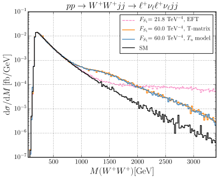
(a) semi logarithmic scale

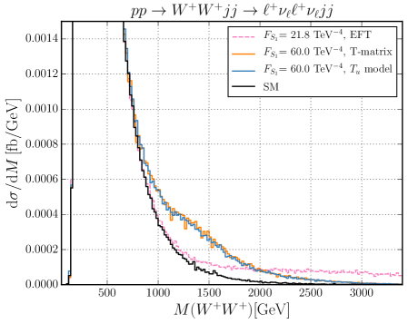
(b) linear scale

Figure 4: Comparison of $T_{u}$ model and linear T-matrix unitarization. Differential cross section as a function of the invariant mass $m_{WW}$ of the weak vector bosons for $pp\rightarrow\ell^{+}\nu_{\ell}\ell^{+}\nu_{\ell}jjX$. The solid black line shows the SM, while the dashed pink line shows the cross section for the $F_{S1}$ anomalous coupling using the present CMS upper limit. The solid orange and blue lines show the a unitarized curve with the same fiducial cross section as the EFT curve using the T-matrix and the $T_{u}$ model, respectively. Cuts defining the fiducial region are given in Eq. (34).

In Fig. 4, we compare the prediction of the naive EFT (dashed pink), the linear T-matrix unitarization (solid orange), the newly introduced $T_{u}$ model (solid blue) and the SM (solid black) for the longitudinal operator $\mathcal{O}_{S_{1}}$ as a function of the invariant mass of the vector boson pair. The coefficient for the naive EFT is chosen as the current experimental limit, $F_{S_{1}}=f_{S_{1}}/\Lambda^{4}=21.8\,{\mathrm{T}eV}^{-4}$, of CMS [6] at $\sqrt{s}=13\,\mathrm{TeV}$. For the unitarized models, T-matrix and $T_{u}$, we choose the coupling such that the fiducial cross section of the naive EFT and the $T_{u}$ model coincide within the VBF cuts of Eq. (34). The number of produced events in the unitarized model are therefore nearly identical to the naive EFT expectation within the high energy region used by CMS to set the experimental bound, and thus the chosen value of $F_{S_{1}}=60\,{\mathrm{T}eV}^{-4}$ approximates the present bound on this coupling for the two unitarized models. Note that the coupling for the unitarized models is approximately a factor 3 larger than for the naive EFT description. The expected excess of events with invariant masses above 2 TeV in the naive EFT description will violate unitarity and is therefore unphysical. Fig. 4b shows that the events of this unphysical high energy tail need to be redistributed to energies between 800 GeV and 2 TeV for the unitarized models, leading to the weaker limit on the Wilson coefficient. Limits on the dimension-8 coefficient derived with the naive EFT model overestimate the sensitivity of experiments to the scale of high energy BSM effects. As displayed in Fig. 4a, the $T_{u}$ model reproduces the linear T-matrix unitarization prescription very well in the high energy range, with barely visible differences at intermediate energies, below $M_{WW}\sim 2$ TeV, which can be traced to subleading effects in $q_{i}^{2}/s$. The deviation of the unitarization models from the SM at high energies is greatly reduced as compared to the naive EFT, and is a valid description beyond the point of unitarity violation in the naive EFT model.

In Table 2, we list the estimated bounds on the full set of dimension-8 coefficients for the $T_{u}$ model, derived as above by matching the fiducial cross section to the one obtained in the naive EFT model. We stress that these numbers should be taken as rough estimates only, to be superseded by full experimental analyses. Their main purpose here is for use in subsequent figures. They illustrate deviations from the SM which are at the edge of what is presently allowed experimentally. The bounds on these Wilson coefficients in the $T_{u}$ model are about a factor of 3 weaker than the corresponding bounds derived within the naive EFT, for all three types of dimension-8 operators. Note, also, that the normalization conventions differ between Éboli and VBFNLO definitions for mixed and transverse operators. In the following we use the notation $F_{i}=f^{\rm Eboli}_{i}/\Lambda^{4}$ for Wilson coefficients of operators ${\cal O}_{i}$ defined with the Éboli normalization.

Measurement	CMS, 13 TeV	Corresponding $T_{u}$	CMS, 13 TeV	Corresponding $T_{u}$
Normalization	Éboli	Éboli	VBFNLO	VBFNLO
$f_{S_{0}}/\Lambda^{4}$	[-7.7,7.7]	[-22,22]	[-7.7,7.7]	[-22,22]
$f_{S_{1}}/\Lambda^{4}$	[-21.6,21.8]	[-50,60]	[-21.6,21.8]	[-50,60]
$f_{M_{0}}/\Lambda^{4}$	[-6.0,5.9]	[-20.0,14.5]	[-14,15]	[-35,49]
$f_{M_{1}}/\Lambda^{4}$	[-8.7,9.1]	[-29,23]	[-22,21]	[-56,71]
$f_{M_{6}}/\Lambda^{4}$	[-11.9,11.8]	[-39,30]	[-29,29]	[-72,94]
$f_{M_{7}}/\Lambda^{4}$	[-13.3,12.9]	[-44,33]	[-31,32]	[-79,107]
$f_{T_{0}}/\Lambda^{4}$	[-0.62,0.65]	[-1.35,1.60]	[-3.7,3.8]	[-8.0, 9.5]
$f_{T_{1}}/\Lambda^{4}$	[-0.28,0.31]	[-0.61,0.85]	[-1.7,1.8]	[-3.6, 5.0]
$f_{T_{2}}/\Lambda^{4}$	[-0.89,1.02]	[-2.1, 2.6]	[-5.3,6.0]	[-12, 15]

Table 2: Experimental limits (in TeV^-4) on dimension-8 operators from the observation of $pp\rightarrow W^{\pm}W^{\pm}jjX$ by CMS [6] (first column) and corresponding estimates for the bounds on the Wilson coefficients $f_{i}/\Lambda^{4}$ in the $T_{u}$ model (second column). Columns three and four give the corresponding numbers for the VBFNLO normalization of operators. See text for further details.

The differential cross section as a function of the invariant mass of the W-pair in Fig. 4 cannot be accessed experimentally, because the 4-momentum of the neutrinos is not measurable. A more readily accessible observable is the differential distribution in the invariant mass of the two charged leptons, which is correlated to a sufficient degree to the invariant mass of the two vector bosons. Fig. 5 shows the corresponding distribution for one non-zero coefficient of each class, namely the longitudinal $\mathcal{O}_{S_{1}}$ (Fig. 5a), the transverse $\mathcal{O}_{T_{0}}$ (Fig. 5b) and the mixed $\mathcal{O}_{M_{0}}$ (Fig. 5c) operator. For all three coefficients, the $T_{u}$ model is suppressed at high energy scales where the EFT description violates unitarity. However, the high energy tails differ by approximately one order of magnitude between the longitudinal operator $\mathcal{O}_{S_{1}}$ and the transverse operator $\mathcal{O}_{T_{0}}$. The differential cross section of the mixed operator in the the $T_{u}$ model lies between these. Below 500 GeV, the event production is mainly driven by SM contributions, as indicated by the fact that the SM curve coincides with the $T_{u}$ model curve for all three operators.

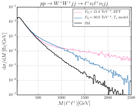
(a) Anomaly due to $\mathcal{O}_{S_{1}}$

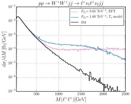
(b) Anomaly due to $\mathcal{O}_{T_{0}}$

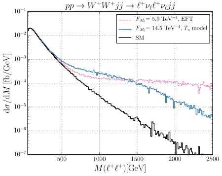
(c) Anomaly due to $\mathcal{O}_{M_{0}}$

Figure 5: Differential cross section as a function of the invariant mass $m_{\ell\ell}$ of the charged leptons for $pp\rightarrow\ell^{+}\nu_{\ell}\ell^{+}\nu_{\ell}jjX$. The solid black line shows the SM, while the dashed pink solid line shows the cross section for the anomalous coupling using the present CMS upper limit. The solid blue line shows the a unitarized curve with the same fiducial cross section as the EFT curve using the $T_{u}$ model. The fiducial region is defined in Eq. (34).

In an attempt to distinguish the different operator types, we study the transverse momentum of the leading tagging jet, $p_{T,\mathrm{max}}(j)$, and the difference of the two lepton transverse momenta, $\Delta p_{T,\ell\ell}=|{\bf p}_{T,\ell_{1}}-{\bf p}_{T,\ell_{2}}|$. To optimize the ratio of BSM to SM events for the following study, Fig. 5 suggests a cut, $m_{\ell^{+}\ell^{+}}>500$ GeV, on the charged lepton pair invariant mass. We show only the transverse and the longitudinal operators in the following and omit the mixed operators, which fall somewhat in between.

In Fig. 6a and Fig. 7a, the differential cross sections as a function of $p_{T,\mathrm{max}}(j)$ and $\Delta p_{T,\ell\ell}$, respectively, are plotted. On the right-hand-side, in Fig. 6b and Fig. 7b the same curves are shown as normalized distributions, which helps to better expose differences in shape. We compare the slope of the SM (solid black), the longitudinal operator $\mathcal{O}_{S_{1}}$ ($T_{u}$: solid blue, naive EFT: dashed pink) and the transverse operator $\mathcal{O}_{T_{0}}$ ($T_{u}$: solid brown, naive EFT: dashed purple).

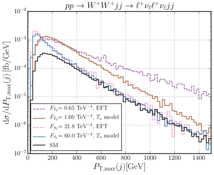
(a) Differential cross section

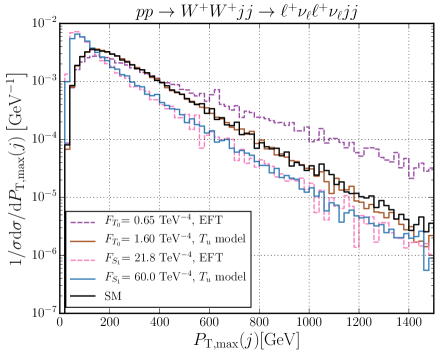
(b) Normalized distribution

Figure 6: Differential cross section as a function of $p_{T,\mathrm{max}}(j)$ for $pp\rightarrow\ell^{+}\nu_{\ell}\ell^{+}\nu_{\ell}jjX$. The solid black line shows the SM, the dashed lines show the naive EFT prediction within present CMS bounds, and the solid blue and brown lines show the corresponding $T_{u}$ model for $\mathcal{O}_{S_{1}}$ and $\mathcal{O}_{T_{0}}$. Beyond the cuts in Eq. (34) we impose $m_{\ell\ell}>500$ GeV.

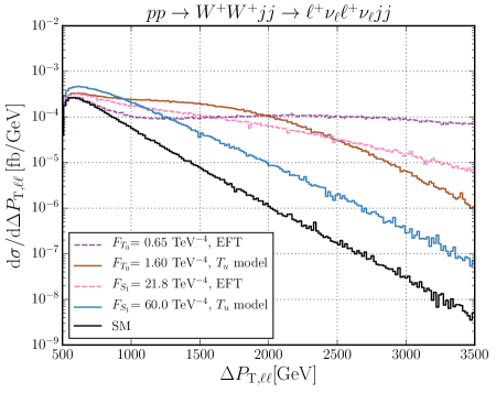
(a) Differential cross section

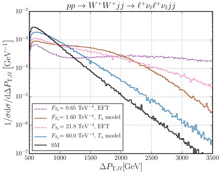
(b) Normalized distribution

Figure 7: Differential cross section as a function of $\Delta p_{T,\ell\ell}$ for $pp\rightarrow\ell^{+}\nu_{\ell}\ell^{+}\nu_{\ell}jjX$. The solid black line shows the SM, the dashed lines show the naive EFT prediction within current CMS bounds, and the solid blue and brown lines show the corresponding $T_{u}$ model for $\mathcal{O}_{S_{1}}$ and $\mathcal{O}_{T_{0}}$. Beyond the cuts in Eq. (34) we impose $m_{\ell\ell}>500$ GeV.

Since incoming transversely polarized weak bosons lead to a harder jet $p_{T}$ distribution than longitudinally polarized bosons [31], and since the transverse operators enhance the transverse components, we expect more events at larger $p_{T,\mathrm{max}}(j)$ for the transverse operators as compared to the longitudinal ones. This is clearly borne out in Fig. 6, which shows a considerably harder $p_{T,\mathrm{max}}(j)$ spectrum for the $\mathcal{O}_{T_{0}}$ operator than for $\mathcal{O}_{S_{1}}$. The cross section enhancement for the longitudinal $\mathcal{O}_{S_{1}}$ operator occurs at small $p_{T}$, which is typical for incident longitudinal bosons. At large $p_{T,\mathrm{max}}(j)$, where incident transversely polarized $W$s dominate, the SM and $\mathcal{O}_{S_{1}}$ curves coincide, indicating that the underlying anomalous quartic gauge coupling is mostly longitudinal.

Anomalous transverse operators produce cross section enhancements also at large $p_{T,\mathrm{max}}(j)$. Here, an interesting difference can be observed between the naive EFT model and our $T_{u}$ model: $T_{u}$ unitarization considerably softens the $p_{T,\mathrm{max}}(j)$ spectrum (dashed purple to solid brown curves). This effect is caused by the suppression of any large enhancement of the $VV\to VV$ partial wave amplitudes, irrespective of its origin. For the transverse operators one finds unphysically large enhancements also at high virtualities of the incoming $W$s, while the $2\to 2$ center of mass energy, $\sqrt{s}=m_{WW}$, remains small. Such an enhancement would not be corrected by a unitarization attempt which relies only on suppression at large $s$, such as the form-factor unitarization implemented previously in VBFNLO. Thus, one needs to be cautious when devising observables for transversely polarized scattering based on a naive EFT approach: The large enhancement at high $p_{T,\mathrm{max}}(j)$ for the purple $\mathcal{O}_{T_{0}}$ curve is an artifact of the missing unitarization. The properly unitarized distribution has a shape which is almost identical to the SM curve in Fig. 6b, which is also dominated by incoming transversely polarized $W$s. Rather, the distinction between incoming longitudinal and transverse weak bosons has to rely on the differences in the $0<p_{T,\mathrm{max}}(j)<200$ GeV region, where, fortunately, also the bulk of the cross section is concentrated in all cases.

A transversely polarized $W^{+}$ with helicity $\lambda=+1$ tends to emit the charged anti-lepton in the forward direction relative to the $W$-momentum, which leads to a high lepton $p_{T}$. This is in contrast to a negatively polarized $W^{+}$, which produces a relatively soft $\ell^{+}$, and the nearly equally shared energy between $\ell^{+}$ and neutrino for the decay of an energetic, longitudinally polarized $W$. Thus, $\Delta p_{T,\ell\ell}$ promises to distinguish $(\lambda_{3},\lambda_{4})=(+,+)$ helicities (high $\Delta p_{T,\ell\ell}$) from e.g. the $(0,0)$ or $(+,-)$ helicity combinations at lower average $\Delta p_{T,\ell\ell}$.

The corresponding differences are clearly exhibited in Fig. 7. Also for the $\Delta p_{T,\ell\ell}$-distribu-tions, the slopes of the dimension-8 operator enhancements are noticeably influenced by the $T_{u}$ model. The unphysical events at larger $\Delta p_{T,\ell\ell}$ are suppressed because $\Delta p_{T,\ell\ell}$ and $\sqrt{s}=m_{WW}$ are highly correlated. The $T_{u}$ model prediction for the longitudinal operators and the SM have more events at $\Delta p_{T,\ell\ell}$ below 1000 GeV and receive a large suppression for larger $\Delta p_{T,\ell\ell}$. As expected, the transverse operator produces a broader distribution, i.e. the enhancement due to $(\lambda_{3},\lambda_{4})=(+,+)$ polarization is clearly visible. For this observable, the unitarization model even increases the discrimination power between different operators types.

5 Discussion and Conclusions

The parameterization of new physics effects in vector boson scattering via anomalous quartic gauge couplings or an effective field theory, including operators up to dimension-8, is a useful tool for analyzing VBS at the LHC. However, because of the large energy reach of hadron colliders, which spans from low energies and momentum transfers where the pure EFT description is valid, to regions of phase space where the polynomial growth of partial wave amplitudes with energy exceeds unitarity limits, the naive EFT description must be generalized to a model which respects unitarity bounds. In this paper, we have developed the $T_{u}$ model, which is one such generalization and which closely mirrors a K-matrix or linear T-matrix unitarization of anomalous VBS amplitudes.

The $T_{u}$ model has been implemented as a purely numerical procedure in the Monte Carlo program VBFNLO [15], which allows to analyze VBS at NLO QCD precision, for arbitrary dimension-8 operators [17]. The $T_{u}$ model is constructed such that it reduces to the naive EFT approximation in all phase space regions where this description is valid, and it smoothly interpolates to a unitarized description for VBS at high virtualities. These high virtualities may either correspond to high boson-pair invariant masses, $m_{V_{3}V_{4}}$, signified by high energy and transverse momentum of the produced vector bosons in $V_{1}V_{2}\to V_{3}V_{4}$, or to highly off-shell incoming $V_{1}$ or $V_{2}$, i.e. large space-like $q_{i}^{2}$, which corresponds to $pp\to V_{3}V_{4}jjX$ events with tagging jets at very high transverse momentum. Unphysical growth of VBS cross sections at high tagging jet $p_{T}$, (see Fig. 6) which is present in a naive EFT implementation even at small $m_{V_{3}V_{4}}$, also needs to be suppressed, and the $T_{u}$ model does provide this regularization.

The purely numerical implementation grants great versatility and avoids analytical approximations, like neglecting $m_{W}^{2}/s$ or $q_{i}^{2}/s$ suppressed terms in a high energy approximation. It allows for arbitrary combinations of dimension-8 operators to be present in the effective Lagrangian and thus provides a general unitarized framework to analyze the effects of dimension-8 operators in VBS at the LHC. In addition, the numerical isolation of off-shell $VV\to VV$ helicity amplitudes at intermediate steps of the calculation, allows, with little additional effort, to generate events for selected center of mass helicities in the BSM $VV\to VV$ contribution, similar to a recent implementation in the PHANTOM Monte Carlo [32, 33]. So far, the implementation of the $T_{u}$ model has been tested and is available for same-sign $W$-boson scattering, more precisely for $pp\rightarrow W^{\pm}W^{\pm}jjX\rightarrow\ell^{\pm}\nu_{\ell}\ell^{\pm}\nu_{\ell}jjX$. However, the generalization to single charged VBS ($WZ$-scattering) and neutral channels will become available soon [34].

For same-sign $W$ scattering we have analyzed distributions which promise a differentiation between individual tensor structures of the operators in the EFT expansion, beyond the only theoretically accessible di-boson invariant mass distribution in Fig. 4 or the invariant mass distribution of the two same-sign charged leptons in Fig. 5. The transverse momentum distribution of the tagging jets, e.g. $p_{T,\mathrm{max}}(j)$, which is shown in Fig. 6 is a good separator between longitudinal and transverse polarization of the incident weak bosons. The charged lepton transverse momentum difference, $\Delta p_{T,\ell\ell}$, which is shown in Fig. 7, can be used to distinguish different combinations of $W$ polarizations in the final state.

For the same-sign $W$ case considered in this paper, we have shown in Fig. 4 that the $T_{u}$ model closely agrees with the T-matrix unitarization discussed by the WHIZARD group [12] for longitudinal $W^{+}W^{+}$ scattering. However, the treatment of subleading, $m_{W}^{2}/s$ or $q_{i}^{2}/s$ suppressed terms is different and means that the two schemes provide different unitarization models. The numerical framework which is now set up in the VBFNLO program allows for easy implementation of variants of the $T_{u}$ model, such as taking into account more than just the largest eigenvalue of the tree level scattering matrix for the denominator when going from Eq. (32) to Eq. (33), or by exploring other mappings of these real eigenvalues onto the Argand circle. We leave such investigations to future work.

References

- [1] H. Georgi. Effective field theory. Ann. Rev. Nucl. Part. Sci., 43:209–252, 1993.
- [2] Celine Degrande, Nicolas Greiner, Wolfgang Kilian, Olivier Mattelaer, Harrison Mebane, Tim Stelzer, Scott Willenbrock, and Cen Zhang. Effective Field Theory: A Modern Approach to Anomalous Couplings. Annals Phys., 335:21–32, 2013.
- [3] Georges Aad et al. Observation of a new particle in the search for the Standard Model Higgs boson with the ATLAS detector at the LHC. Phys. Lett., B716:1–29, 2012.
- [4] Serguei Chatrchyan et al. Observation of a new boson at a mass of 125 GeV with the CMS experiment at the LHC. Phys. Lett., B716:30–61, 2012.
- [5] O. J. P. Eboli, M. C. Gonzalez-Garcia, and J. K. Mizukoshi. and at and for the study of the quartic electroweak gauge boson vertex at CERN LHC. Phys. Rev., D74:073005, 2006.
- [6] Albert M. Sirunyan et al. Observation of electroweak production of same-sign W boson pairs in the two jet and two same-sign lepton final state in proton-proton collisions at 13 TeV. Phys. Rev. Lett., 120(8):081801, 2018.
- [7] Vardan Khachatryan et al. Study of vector boson scattering and search for new physics in events with two same-sign leptons and two jets. Phys. Rev. Lett., 114(5):051801, 2015.
- [8] Morad Aaboud et al. Measurement of vector-boson scattering and limits on anomalous quartic gauge couplings with the ATLAS detector. Phys. Rev., D96(1):012007, 2017.
- [9] Thomas Appelquist and Guo-Hong Wu. The Electroweak chiral Lagrangian and new precision measurements. Phys. Rev., D48:3235–3241, 1993.
- [10] Marco Sekulla, Wolfgang Kilian, Thorsten Ohl, and Jürgen Reuter. Effective Field Theory and Unitarity in Vector Boson Scattering. PoS, LHCP2016:052, 2016.
- [11] Michael Rauch. Vector-Boson Fusion and Vector-Boson Scattering. 2016. arXiv:1610.08420.
- [12] Wolfgang Kilian, Thorsten Ohl, Jürgen Reuter, and Marco Sekulla. High-Energy Vector Boson Scattering after the Higgs Discovery. Phys. Rev., D91:096007, 2015.
- [13] Wolfgang Kilian, Thorsten Ohl, Jürgen Reuter, and Marco Sekulla. Resonances at the LHC beyond the Higgs boson: The scalar/tensor case. Phys. Rev., D93(3):036004, 2016.
- [14] Ana Alboteanu, Wolfgang Kilian, and Juergen Reuter. Resonances and Unitarity in Weak Boson Scattering at the LHC. JHEP, 11:010, 2008.
- [15] K. Arnold et al. VBFNLO: A Parton level Monte Carlo for processes with electroweak bosons. Comput. Phys. Commun., 180:1661–1670, 2009. arXiv:0811.4559.
- [16] J. Baglio et al. VBFNLO: A Parton Level Monte Carlo for Processes with Electroweak Bosons – Manual for Version 2.7.0. 2011. arXiv:1107.4038.
- [17] J. Baglio et al. Release Note - VBFNLO 2.7.0. 2014. arXiv:1404.3940.
- [18] Gerhard Buchalla, Oscar Cata, and Claudius Krause. Complete Electroweak Chiral Lagrangian with a Light Higgs at NLO. Nucl. Phys., B880:552–573, 2014. [Erratum: Nucl. Phys.B913,475(2016)].
- [19] Thomas Appelquist and Claude W. Bernard. Strongly Interacting Higgs Bosons. Phys. Rev., D22:200, 1980.
- [20] Anthony C. Longhitano. Heavy Higgs Bosons in the Weinberg-Salam Model. Phys. Rev., D22:1166, 1980.
- [21] W. Buchmüller and D. Wyler. Effective Lagrangian Analysis of New Interactions and Flavor Conservation. Nucl. Phys., B268:621–653, 1986.
- [22] Kaoru Hagiwara, S. Ishihara, R. Szalapski, and D. Zeppenfeld. Low-energy effects of new interactions in the electroweak boson sector. Phys. Rev., D48:2182–2203, 1993.
- [23] B. Grzadkowski, M. Iskrzynski, M. Misiak, and J. Rosiek. Dimension-Six Terms in the Standard Model Lagrangian. JHEP, 10:085, 2010.
- [24] M. Baak et al. Working Group Report: Precision Study of Electroweak Interactions. In Proceedings, 2013 Community Summer Study on the Future of U.S. Particle Physics: Snowmass on the Mississippi (CSS2013): Minneapolis, MN, USA, July 29-August 6, 2013, 2013.
- [25] C. Itzykson and J. B. Zuber. Quantum Field Theory. International Series In Pure and Applied Physics. McGraw-Hill, New York, 1980.
- [26] G. Perez R. Unitarization models for vector boson scattering at the lhc. 2018. Available at https://publikationen.bibliothek.kit.edu/1000082199.
- [27] M. Loeschner. Unitarisation of anomalous couplings in vector boson scattering. 2014. Available at https://www.itp.kit.edu/prep/diploma/PSFiles/Master_Max.pdf.
- [28] S. Brass, C. Fleper, W. Kilian, J. Reuter, and M. Sekulla. Transversal Modes and Higgs Bosons in Electroweak Vector-Boson Scattering at the LHC. 2018. SI-HEP-2018-17.
- [29] Matteo Cacciari, Gavin P. Salam, and Gregory Soyez. The Anti-k(t) jet clustering algorithm. JHEP, 04:063, 2008.
- [30] Hung-Liang Lai, Marco Guzzi, Joey Huston, Zhao Li, Pavel M. Nadolsky, Jon Pumplin, and C. P. Yuan. New parton distributions for collider physics. Phys. Rev., D82:074024, 2010.
- [31] Sally Dawson. The Effective W Approximation. Nucl. Phys., B249:42–60, 1985.
- [32] Alessandro Ballestrero, Ezio Maina, and Giovanni Pelliccioli. boson polarization in vector boson scattering at the LHC. JHEP, 03:170, 2018.
- [33] Alessandro Ballestrero, Aissa Belhouari, Giuseppe Bevilacqua, Vladimir Kashkan, and Ezio Maina. PHANTOM: A Monte Carlo event generator for six parton final states at high energy colliders. Comput. Phys. Commun., 180:401–417, 2009.
- [34] H. Schäfer-Siebert, M. Sekulla, and D. Zeppenfeld. in preparation.