Local convergence for permutations and local limits for uniform -avoiding permutations with
Abstract.
We set up a new notion of local convergence for permutations and we prove a characterization in terms of proportions of consecutive pattern occurrences. We also characterize random limiting objects for this new topology introducing a notion of “shift-invariant” property (corresponding to the notion of unimodularity for random graphs).
We then study two models in the framework of random pattern-avoiding permutations. We compute the local limits of uniform -avoiding permutations, for when the size of the permutations tends to infinity. The core part of the argument is the description of the asymptotics of the number of consecutive occurrences of any given pattern. For this result we use bijections between -avoiding permutations and rooted ordered trees, local limit results for Galton–Watson trees, the Second moment method and singularity analysis.
Key words and phrases:
Local weak limits, permutation patterns2010 Mathematics Subject Classification:
60C05,05A051. Introduction
The goal of this article is to introduce a local topology for permutations and to study some initial interesting applications.
1.1. Scaling and local limits for discrete structures
It is well-known that, after a suitable rescaling, a simple random walk on converges to the 1-dimensional Brownian motion: probably this is the most famous scaling limit result in probability theory. In the last thirty years such scaling limits have been intensively studied for different discrete structures. We mention some mathematical areas where this notion has been investigated, without aiming at giving a complete list.
In the framework of random trees and planar maps, the systematic study of scaling limits has been initiated by Aldous with the pioneering series of articles about the well-known Continuum random tree ([3, 4, 5]). After that, many new results have been proven, in particular about the Brownian map, which is the scaling limit of random planar maps uniformly distributed over the class of all rooted -angulations with faces, for and even integer (see for instance [41, 45, 46]).
In statistical mechanics, the study of scaling limits of discrete models is also a very active topic. For instance, the scaling limit of the discrete Gaussian free field on lattices, i.e., the continuum GFF, has been proven to be the scaling limit of many others random structures (see for instance [37, 52]).
More closely related to this work, in [30] a notion of scaling limits for permutations has been recently introduced, called permutons. They are probability measures on the unit square with uniform marginals, and they represent the scaling limit of the diagram of permutations as the size grows to infinity. This new notion of convergence has been studied (sometimes phrased in other terms) in several works. We mention a few of them.
-
•
The study of the scaling limits of a uniform random permutation avoiding a pattern of length three was initiated by Miner and Pak [47] and Madras and Pehlivan [44]. Next, with a series of two articles, Hoffman, Rizzolo and Slivken ([26, 27]) strengthened these early results and understood many interesting phenomena that had previously gone unexplained. In particular they explored the connection of these uniform pattern-avoiding permutations to Brownian excursions. All these articles do not use the “permuton language”.
-
•
The first concrete and explicit example of convergence in the “permuton language” has been studied by Kenyon, Kral, Radin and Winkler [38]. They studied scaling limits of random permutations in which a finite number of pattern densities have been fixed.
- •
-
•
In a second work, Bassino, Bouvel, Féray, Gerin, Maazoun and Pierrot [9] showed that the Brownian permuton has a universality property: they consider uniform random permutations in proper substitution-closed classes and study their limiting behavior in the sense of permutons, showing that the limit is an elementary one-parameter deformation of the Brownian separable permuton.
-
•
With a statistical mechanical approach , Starr [53] investigates the permuton limit of Mallows permutations. This is a non-uniform model where the probability of every permutation is proportional to . Treating the question as a mean-field problem, he is able to calculate the distribution of the permuton limit (after a suitable rescaling of the parameter ).
-
•
Rahman, Virag and Vizer [51] generalized the study of scaling limits for permutations to permutation valued processes, i.e., sequences of sequences of permutations.
-
•
Permutons limits have been characterized in terms of convergence of frequencies of pattern occurrences (see [9, Theorem 2.5]). We will come back later to this characterization.
In parallel to scaling limits, a second notion of limits of discrete structures, on which this paper focuses, has been introduced: the local limits. Informally, scaling limits look at the convergence of the objects from a global point of view (after a rescaling of the distances between points of the objects), while local limits look at discrete objects in a neighborhood of a distinguished point (without rescaling distances). As done for scaling limits, we allude to some frameworks where this notion has been studied, again without aiming at giving a complete overview.
Local limit results around the root of random trees were first implicitly proved by Otter [49] and then explicitly by Kesten [39] and Aldous and Pitman [6]. Janson [32] gives a unified treatment of the local limits, as the number of vertices tends to infinity, of simply generated random trees. Recently, Stufler [55] studied also the local limits for large Galton–Watson trees around a uniformly chosen vertex building on previous results of Aldous [2] and Holmgren and Janson [29].
Although implicit in many earlier works, the notion of local convergence around a random vertex (called weak local convergence) for random graphs has been formally introduced by Benjamini and Schramm [11] and Aldous and Steele [7]. One would expect that a limit object for this topology should “look the same” when regarded from any of its vertices (because of the uniform choice of the root). This property is made precise by the notion of unimodular random rooted graph and the weak local limit of any sequence of random graphs is indeed proven to be unimodular (see [11]).
Also in the framework of random planar maps the local convergence has been studied. For example, a well-known result is that the local limit for random infinite triangulations/quadrangulations is the uniform infinite planar triangulation/quadrangulation (UIPT/UIPQ) (see for instance [8, 40, 54]).
In the framework of permutations, to the best of our knowledge, a local limit approach has not been investigated so far. The goal of the current paper is to fill this gap and show several interesting aspect of the local convergence for permutations. More precisely,
-
•
we prove a characterization of the local convergence in terms of proportions of consecutive pattern occurrences (see Theorems 1.3 and 1.5). For the sake of comparison, recall that permutons limits have been characterized in terms of convergence of frequencies of (non-consecutive) pattern occurrences.
-
•
We characterize random limiting objects for this new topology (see Theorem 1.7), introducing a notion of “shift-invariant” property (corresponding to the notion of unimodularity for random graphs).
- •
Remark 1.1.
We wish to mention that Hoffman, Rizzolo and Slivken [28] used local limits results for random trees in the study of some specific properties of permutations, like the number of fixed points (i.e., indexes such that ) of pattern-avoiding permutations. Moreover, they do not study general local limits results for permutations.
Remark 1.2.
We also mention that recently Pinsky [50] studied limits of random permutations avoiding patterns of size three considering a different topology. His topology captures the local limit of the permutation diagram around a corner. The two topologies (that from [50] and that from the present article) are not comparable. We point out that there are two main advantages to our definition of local limits: first, convergence for our local topology is pleasantly equivalent to the convergence of consecutive pattern proportions; second, many natural models have an interesting limiting object for our topology (while converging to in the topology of [50]).
The reader not familiar with the terminology of permutation patterns (such as pattern occurrences, pattern avoidance, etc.) can find the necessary background in Section 2.1.
1.2. Overview of our results
Our work can be divided into two main parts.
1.2.1. Local convergence for permutations
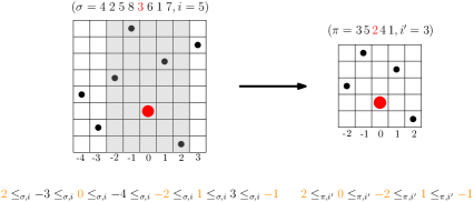
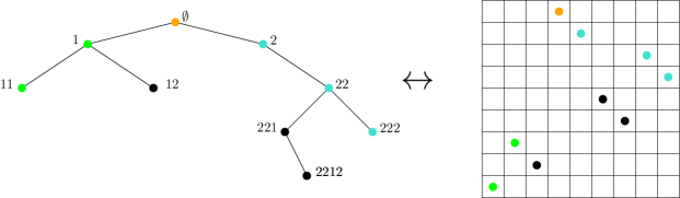
In the first part (Section 2) we develop the theory of local convergence for permutations. We will often view a permutation as a diagram, i.e., the set of points of the Cartesian plane at coordinates (see Fig. 1 for an example). In the context of local convergence we need to look at permutations with a distinguished entry, called root. Denoting with the set of permutations of size , we say that a pair is a finite rooted permutation of size if and .
To a rooted permutation , we associate a total order on a finite interval of integers containing 0 denoted by The total order is simply obtained from the diagram of (as shown in the left-hand side of Fig. 1). We shift the indices of the -axis in such a way that the column containing the root of the permutation has index zero (the new indices are reported under the columns of the diagram). Then we set if the point in column is lower than the point in column
Since this correspondence defines a bijection, we identify every rooted permutation with the total order . Thanks to this identification, it is natural to call infinite rooted permutation a pair where is an infinite interval of integers containing 0 and is a total order on .
In order to define a notion of local convergence, we introduce a notion of -restriction around the root. It can be thought of as the diagram of the pattern induced by a “vertical strip” of width around the root of the permutation (see Fig. 1) or equivalently of the restriction of the order to Note that this second equivalent characterization trivially applies also to infinite rooted permutations.
Then we say that a sequence of rooted permutations is locally convergent to a rooted permutation if, for all the -restrictions of the sequence converge to the -restriction of (see Definition 2.11 for a formal statement).
We extend this notion of local convergence for rooted permutations to (unrooted) permutations, rooting them at a uniformly chosen index of . With this procedure, a fixed permutation naturally identifies a random variable that takes values in the set of finite rooted permutations (here and throughout the paper we denote random quantities using bold characters). In this way, the following notion of weak local convergence is natural: given a sequence of permutations , we say that Benjamini–Schramm converges to a random possibly infinite rooted permutation if the sequence where is a uniform index in , converges in distribution to with respect to the above defined local topology. We point out that our choice for the terminology comes from the analogous notion for graphs (see [11]).
We prove the following characterization in terms of proportions of consecutive pattern occurrences (for a formal and complete statement see Theorem 2.19). For any pattern of size , and any permutation of size , we denote by
the proportion of consecutive occurrences of in Moreover, we denote with the set of permutations of finite size.
Theorem 1.3.
For any , let be a permutation of size . Then the Benjamini–Schramm convergence for the sequence is equivalent to the existence of non-negative real numbers such that, for all patterns ,
Remark 1.4.
We could have introduced local convergence for permutations also from another point of view, closer to the one developed for graphons (see [42]): we could say that a sequence of permutations is locally convergent if for every pattern the sequences converge and then characterize the limiting objects. Theorem 1.3 shows that the two approaches are equivalent.
What makes Theorem 1.3 particularly interesting is the intense study of consecutive patterns. This is a very active field both from a combinatorial and a probabilistic point of view, with applications in computer science, biology, and physics. Classical statistics like the number of descents, runs and peaks contained in a permutation can be viewed as particular examples of consecutive patterns in permutations, but more general approaches have been developed, for example concerning the asymptotic behavior of the number of permutations avoiding a consecutive pattern. For a complete overview, we refer to the wonderful survey on the topic by Elizalde [23].
Once the Benjamini–Schramm convergence has been introduced for sequences of deterministic permutations, we then extend this notion to sequences of random permutations The presence of two sources of randomness, one for the choice of the permutation and one for the (uniform) choice of the root, leads to two non-equivalent possible definitions: the annealed and the quenched version of the Benjamini–Schramm convergence (see Definitions 2.20 and 2.27). Intuitively, in the second definition, the random permutation is frozen, whereas in the first one, the random permutation and the choice of the root are treated on the same level.
We obtain the following two additional characterizations (for formal and complete statements see Theorems 2.24 and 2.32).
Theorem 1.5.
For any , let be a random permutation of size . Then
-
(a)
the annealed version of the Benjamini–Schramm convergence of is equivalent to the existence of non-negative real numbers such that
-
(b)
The quenched version of the Benjamini–Schramm convergence of is equivalent to the existence of non-negative real random variables such that
w.r.t. the product topology (where indicates the convergence in distribution).
Obviously, the quenched version implies the annealed version.
Remark 1.6.
The idea of defining and studying the quenched Benjamini–Schramm convergence is motivated by the theorem above. Indeed, one of the main goal for introducing the local topology was to obtain the characterization stated in point (b). We point out that the quenched Benjamini–Schramm convergence has been considered also for random trees (see for instance [22]). The terminology “annealed/quenched” is classical in statistical mechanics in the study of random systems on random environments.
At this point we want to highlight a remarkable difference with the case of permuton convergence and its characterization mentioned before. Indeed, for the proportion of (non-consecutive) occurrences of patterns, the convergences in (a) and (b) are equivalent as shown in [9, Theorem 2.5]. On the other hand, in Example 2.36 we show that the annealed and quenched version of the Benjamini–Schramm convergence are not equivalent.
Finally, we are also able to characterize random limiting objects for the annealed version of the Benjamini–Schramm convergence introducing a “shift-invariant” property. For an order its shift is defined by if and only if A random infinite rooted permutation, or equivalently a random total order, is said to be shift-invariant if it has the same distribution than its shift (for precise statements see Definition 2.41, Proposition 2.44 and Theorem 2.45).
Theorem 1.7.
A random infinite rooted permutation is “shift-invariant” if and only if it is the local limit of a sequence of random permutations in the annealed Benjamini–Schramm sense.
In some sense, our “shift-invariant” property corresponds to the notion of unimodularity for random graphs. As said before, it is well-known that the Benjamini–Schramm limit of a sequence of random graphs is unimodular. However, it is an open problem to determine if every unimodular random graph is the local limit of a sequence of finite random graphs rooted uniformly at random.
1.2.2. Local limits for uniform -avoiding permutations with
In the second part of the article (Sections 4 and 5), we demonstrate the relevance of this new notion of convergence. As first models for studying local convergence, we consider some classes of pattern avoiding permutations. This choice is motivated by the intense study of permutation classes in the last thirty/forty years. For a great survey we refer to Vatter [56]. In general, they have been deeply studied from a combinatorial point of view, finding the enumeration of specific classes. The most basic result in the field is that the number of -avoiding permutations of size , for is given by the -th Catalan number.
More recently a new probabilistic approach to the study of permutation classes has been investigated. An example, as explained in the previous section, is the study of scaling limits of uniform random permutations in a fixed pattern-avoiding class. Another example is the general problem of studying the limiting distribution of the number of occurrences (after a suitable rescaling) of a fixed pattern in a uniform random permutation belonging to a fixed class when the size tends to infinity (see for instance Janson [34, 33, 35] where the author studied this problem in the model of uniform permutations avoiding a fixed family of patterns of size three).
In this work we focus on the classes of -avoiding permutations, for since several bijections (see for instance [20]) with other combinatorial objects (such as rooted ordered trees and Dyck paths) are known and we expect some connection between the local limit convergence for trees and the local limit convergence for permutations.
Our two main results of this second part are the two following theorems.
Theorem 1.8.
For any , let be a uniform random -avoiding permutation of size . Then we have the following convergence in probability,
| (1) |
where (resp. ) denotes the number of left-to-right maxima (resp. right-to-left maxima) in .
Theorem 1.9.
For any , let be a uniform random -avoiding permutation of size . Then we have the following convergence in probability for all ,
| (2) |
Observation 1.10.
By symmetry, this covers all cases of -avoiding permutations with Indeed, every permutation of size three is in the orbit of either or by applying reverse (symmetry of the diagram w.r.t. the vertical axis) and complementation (symmetry of the diagram w.r.t. the horizontal axis). Beware that inverse (symmetry of the diagram w.r.t. the principal diagonal) cannot be used since it does not preserve consecutive pattern occurrences.
Since the limits of the random sequences are deterministic, for all patterns , the convergence in probability in (1) and (2) is equivalent to the convergence in distribution of the vectors for the product topology. Therefore Theorems 1.8 and 1.9 trivially imply the characterization in Theorem 1.5 and so prove that the sequences converge for the quenched version, i.e., the stronger version, of the Benjamini–Schramm convergence.
Here are some other interesting aspects of Theorems 1.8 and 1.9.
-
•
A first important fact is the concentration phenomenon, namely the fact that the limits of the random sequences are deterministic, for all pattern . Indeed Janson [34, Remark 1.1] notices that, in some classes, we have concentration for the (non-consecutive) pattern occurrences around their mean, in others not. It would be interesting to understand in a more general setting when this concentration phenomenon does or does not occur (we will come back to this fact in the next section).
-
•
The second important fact is the different behavior of the two models of Theorem 1.8 and Theorem 1.9: the first limiting density has full support on the space of 231-avoiding permutations, whereas the second gives positive measure only to 321-avoiding permutations whose inverse have at most one descent. Indeed, despite having the same enumeration sequence, and are often considered in the community as behaving really differently. Our results give new evidence of this belief.
- •
Although the two theorems have very similar statements and in both models we use bijections between -avoiding permutations and rooted ordered trees, the two proofs involve different techniques.
-
•
For the proof of Theorem 1.8 we use the Second moment method. We study the asymptotic behavior of the first and the second moments of applying a technique introduced by Janson [33, 31]. Instead of studying uniform trees with vertices, we focus on specific families of binary Galton–Watson trees (which have some nice independence properties). Then we recover results for the first family of trees using singularity analysis for generating functions.
-
•
For the proof of Theorem 1.9 we use a probabilistic approach for the study of local limits for Galton–Watson trees pointed at a uniform vertex. The bijection between trees and 321-avoiding permutations that we used, strongly depends on the position of the leaves. We therefore study the contour functions of some specific Galton–Watson trees in order to extract information about the positions of the leaves in the neighborhood of a uniform vertex.
1.3. Future projects and open problems
We believe that this new notion of local convergence for permutations is worth being further investigated in several ways. We list our ideas for future projects.
-
•
Motivated by the work of Janson [34] we would like to extend our results to uniform permutations avoiding multiple patterns. In the case of patterns of size three, this generalization does not contain any difficulty (due to the high level of independence for the values of a uniform permutation in these classes) and the explicit analysis of the problem has been developed in the bachelor thesis of Petrella under the supervision of Barbato at the University of Padua.
-
•
We would like to generalize the proof of Theorem 1.9 for all uniform -avoiding permutation when is an increasing or decreasing permutation of size greater than three.
-
•
We studied the local convergence for uniform permutations in some classes. Another interesting direction could be to study non-uniform models. Motivated by the work of Crane, DeSalvo and Elizalde [21] we believe that the local limit of random permutations with Mallows distribution could be investigated. More generally, we would like to investigate different types of biased models.
-
•
In a work with Bouvel, Féray and Stufler [18] we investigate local limits for uniform permutations in substitution-closed classes. Also in this setting, the concentration phenomenon for the proportions of consecutive pattern occurrences occurs.
-
•
A challenging problem (motivated by the previous results) is to find natural (but non-trivial) models where there is no concentration for the proportion of consecutive pattern occurrences (for a trivial model see Example 2.36).
Note added in revision: A first family of permutations where there is no concentration phenomenon has been recently investigated in [19] by the author and Slivken.
-
•
In a more theoretical direction we would like to examine in depth the relationship between local convergence and permuton convergence (and other possible intermediate notion of convergence for permutations, as done for example in [25] for graphs).
-
•
As said before we are able to characterize random limiting objects for the annealed version of the Benjamini–Schramm convergence. It would be interesting to find a similar characterization for the stronger quenched version, where the limiting objects are random probability measures.
1.4. Outline of the paper
The paper is organized as follows:
2. Local convergence for permutations
2.1. Permutations and patterns
We introduce some notation to be used in the sequel. For any we denote the set of permutations of by We write permutations of in one-line notation as For a permutation the size of is denoted by We let be the set of finite permutations. We write sequences of permutations in as
If is a sequence of distinct numbers, let be the unique permutation in that is in the same relative order as i.e., if and only if Given a permutation and a subset of indices , let be the permutation induced by namely, For example, if and then .
Given two permutations for some and for some we say that contains as a pattern if has a subsequence of entries order-isomorphic to that is, if there exists a subset such that In addition, we say that contains as a consecutive pattern if has a subsequence of adjacent entries order-isomorphic to that is, if there exists an interval such that All the intervals considered in the article are to be understood as integer intervals, i.e., intervals contained in and will be denoted by for
Example 2.1.
The permutation contains as a pattern but not as a consecutive pattern and as consecutive pattern. Indeed but no interval of indices of induces the permutation Moreover,
We say that avoids if does not contain as a pattern. We point out that the definition of -avoiding permutations refers to patterns and not to consecutive patterns. We denote by the set of -avoiding permutations of size and by the set of -avoiding permutations of arbitrary size.
We denote by the number of consecutive occurrences of a pattern in More precisely
where denotes the cardinality of a set. Moreover, we denote by the proportion of consecutive occurrences of a pattern in that is,
Remark 2.2.
The natural choice for the denominator of the previous expression should be and not but we make this choice for later convenience (for example, in order to give a probabilistic interpretation of the quantity as done in Equation (12, p.12). Moreover, for every fixed there are no difference in the asymptotics when tends to infinity.
2.2. The set of rooted permutations
In the first part of this section we define the notion of finite and infinite rooted permutation. Then we introduce a local distance and at the end we show that the space of (possibly infinite) rooted permutations is the natural space to study local limits of permutations. More precisely, we show that this space is compact and it contains the space of finite rooted permutations as a dense subset.
For the reader convenience, we recall the following fundamental definition.
Definition 2.3.
A finite rooted permutation is a pair where and for some
We extend the notion of size of a permutation to rooted permutations in the natural way, i.e., We denote with the set of rooted permutations of size and with the set of finite rooted permutations. We write sequences of finite rooted permutations in as
To a rooted permutation we associate the pair where is a finite interval containing 0 and is a total order on defined for all by
Clearly this map is a bijection from the space of finite rooted permutations to the space of total orders on finite integer intervals containing zero. Consequently and throughout the paper, we identify every rooted permutation with the total order
We want to highlight in the following example that the total order associated to a rooted permutation indicates how the elements of at given positions compare to each other.
In most examples, we draw permutations as diagrams. We recall that the diagram of a permutation of size is the set of points of the Cartesian plane at coordinates for . For a rooted permutation we draw the root with a bigger red dot at coordinates
Example 2.4.
The diagram of the rooted permutation is provided in the left-hand side of Fig. 2. The associated total order is where
Observation 2.5.
A total order (associated to a rooted permutation ) shifted to the interval seen as a word coincides with the inverse permutation
For instance, the total order in Example 2.4 shifted on the interval gives The word corresponding to it coincides with the inverse permutation
Thanks to the identification between rooted permutations and total orders, the following definition of an infinite rooted permutation is natural.
Definition 2.6.
We call infinite rooted permutation a pair where is an infinite interval of integers containing 0 and is a total order on . We denote the set of infinite rooted permutations by
We highlight that infinite rooted permutations can be thought of as rooted at 0. We set
namely, the set of finite and infinite rooted permutations and we denote by the set of rooted permutations with size at most We write sequences of finite or infinite rooted permutations in as
We now introduce the following restriction function around the root defined, for every , as follow
| (3) |
We can think of restriction functions as a notion of neighborhood around the root. For finite rooted permutations we also have the equivalent description of the restriction functions in terms of consecutive patterns: if then where and
In the next example we give a graphical interpretation of the restriction function around the root.
Example 2.7.
We continue Example 2.4 with the rooted permutation When we consider the restriction we draw in gray a vertical strip “around” the root of width (or less if we are near the boundary of the diagram). An example is provided in Fig. 3 where is computed. In particular with
We now introduce a last definition.
Definition 2.8.
We say that a family of elements in is consistent if
We have the following.
Observation 2.9.
For every infinite rooted permutation the corresponding family of restrictions is consistent.
In the next example, we exhibit a concrete infinite rooted permutation, with some of its restrictions and the associated rooted permutations.
Example 2.10.
We consider the following total order on
that is, the standard order on the integers except that the order on negative numbers is reversed and negative even numbers are smaller than negative odd numbers. Using the definition given in Equation we have for
which represents the rooted permutation for whose diagram is represented in the left-hand side of Fig. 4. In particular,
Moreover, for
which represents the rooted permutation for whose diagram is represented in the right-hand side of Fig. 4. In particular, We also note that as shown in Fig. 4.
2.3. Local convergence for rooted permutations
We are now ready to define a notion of local distance on the set of (possibly infinite) rooted permutations . Given two rooted permutations we define
| (4) |
with the classical conventions that and It is a basic exercise to check that is a distance. Actually, is ultra metric, and so all the open balls of radius centered in – which we denote by – are closed and intersecting balls are contained in each other. We will say that the balls are clopen, i.e., closed and open.
Once we have a distance, the following notion of convergence is very natural.
Definition 2.11.
We say that a sequence of rooted permutations in is locally convergent to an element if it converges with respect to the local distance In this case we write
We are now going to show that the space is the right space to consider in order to study the limits of finite rooted permutations with respect to the local distance defined in Equation (4). More precisely, as explained at the beginning, we show that is compact and that is dense in
The latter assertion is trivial since
| (5) |
and obviously
Before proving compactness we explore some basic but important properties of our local distance . The next proposition gives a converse to Observation 2.9.
Proposition 2.12.
Given a consistent family of elements in there exists a unique (possibly infinite) rooted permutation such that
Moreover,
Proof.
We explicitly construct the rooted permutation We set From the consistency property of the family we immediately deduce that for all and so the set is an interval of Moreover, the set trivially contains 0. In order to construct a (possibly infinite) permutation we have to endow the interval with a total order For all we set and we make the following choice:
| (6) |
Note that the transitivity of easily follows from the consistency property.
By construction, for all and so we can conclude that the sequence locally converges to Uniqueness follows from the uniqueness of the limit in a metric space. ∎
Proposition 2.12 allows us to see the space as a subset of a product space of finite sets as explained in the following observation.
Observation 2.13.
We consider the product space endowed with the product topology, that is metrizable by the distance
We have the following isometric embedding
| (7) |
with inverse
| (8) |
We note that is well-defined and coincides with the inverse of thanks to Proposition 2.12. Moreover, the embedding is isometric since obviously the two distances coincide on and
Therefore, is homeomorphic to
Since and are homeomorphic, then the corresponding notions of convergence are equivalent. An immediate consequence is the following.
Proposition 2.14.
Given a sequence of rooted permutations in the following are equivalent:
-
(a)
there exists such that
-
(b)
there exists a family of finite rooted permutations such that
In particular if one of the two conditions holds (and so both), then for all
Observation 2.15.
Note that for all the restriction functions are continuous. This is a simple consequence of implication in the previous proposition.
We end this section with the following.
Theorem 2.16.
The metric space is compact.
Proof.
By Proposition 2.12, is the set of consistent sequences. Therefore, it is an intersection of clopen subsets (the sets of sequences that are consistent in the first restrictions) of the compact product space Therefore is compact and so also since they are homeomorphic. ∎
2.4. Benjamini–Schramm convergence: the deterministic case
In this section we want to define a notion of weak-local convergence for a deterministic sequence of finite permutations The case of a random sequence will be discussed in Section 2.5.
Some of the results contained in this section are just special cases of the those in Section 2.5.1 about the annealed version of the Benjamini–Schramm convergence. However we choose to present the deterministic case separately with a double purpose: first, in this way, the definitions are clearer, secondly, we believe that the subsequent quenched version of the Benjamini–Schramm convergence (see Section 2.5.2) will be more intuitive.
A possible way to define this weak-local convergence is to use the notion of local distance defined in Equation Therefore, we need to construct a sequence of rooted permutations from the sequence We can see a fixed permutation as an element of only after a root has been chosen. A natural way to choose a root is to make the choice at random, and uniformly among the indices of In this way, a fixed permutation naturally identifies a probability measure on the space that is
| (9) |
where is a uniform index of Equivalently, the measure is the law of the random variable that takes values in the set
Notation 2.17.
In order to avoid any confusion, as done in Equation (9), we write random quantities using bold characters to distinguish them from deterministic quantities. Moreover, given a probability measure we denote with the expectation with respect to and given a random variable we denote with its law. Given a sequence of random variables we write to denote the convergence in distribution and to denote the convergence in probability. Finally, given an event we denote with the complement event of
We are now ready to define our notion of Benjamini–Schramm convergence for sequences of permutations.
Definition 2.18.
Given a sequence of elements in we say that Benjamini–Schramm converges to a random (possibly infinite) rooted permutation , if the sequence where is a uniform index of converges in distribution to with respect to the local distance defined in Equation In this case we simply write instead of
Sometimes, in order to simplify notation, we will denote the Benjamini–Schramm limit of a sequence simply by instead of
Our main theorem in this section deals with the following interesting relation between the Benjamini–Schramm convergence and the convergence of consecutive pattern densities.
Theorem 2.19.
For any let be a permutation of size Then the following are equivalent:
-
(a)
there exists a random rooted infinite permutation such that
-
(b)
there exist non-negative real numbers such that for all patterns
Moreover, if one of the two conditions holds (and so both) we have the following relation between the limiting objects:
We skip for the moment the proof of this theorem since it will be a particular case of the more general Theorem 2.24.
2.5. Benjamini–Schramm convergence: the random case
The goal of this section is to characterize the convergence in distribution of a sequence of random permutations with respect to the local distance defined in Equation (4). We have two different natural choices for this definition, one stronger than the other (and not equivalent as shown in Example 2.36). The weaker definition is an analogue of the notion of Benjamini–Schramm convergence for random graphs developed in [11].
Before starting, we give some more explanations about our notation for random quantities. We will use a superscript notation on probability measure (and on the corresponding expectation ) to record the source of randomness. Specifically, given two independent random variables and (with values in two spaces and respectively) and a set we write
and similarly
Moreover, we recall the following standard relation
| (10) |
2.5.1. The annealed version of the Benjamini–Schramm convergence
In analogy with the definition of Benjamini–Schramm convergence for deterministic sequences of permutations (and the definition of Benjamini–Schramm convergence for graphs) we can state the following.
Definition 2.20 (Annealed version of the Benjamini–Schramm convergence).
Given a sequence of random permutations in let be a uniform index of conditionally on . We say that converges in the annealed Benjamini–Schramm sense to a random variable with values in if the sequence of random variables converges in distribution to with respect to the local distance. In this case we write instead of
Like in the deterministic case, the limiting object is a random rooted infinite permutation.
Remark 2.21.
Even though the above definition is stated for sequences of random permutations of arbitrary size, we will often consider the case when, for all almost surely and the random choice of the root is uniform in and independent of .
Before stating the main theorem of this section we clarify two interesting properties of the statistics introduced in Section 2.1.
Given a permutation we set
In the following example we give a graphical interpretation of the operation .
Example 2.22.
Let then where we highlight in light blue the entries already presented in the permutation
Now, for all and with we just observe that
| (11) |
and so the convergence of depends only on the convergence of for all
We also give a probabilistic interpretation of for and with Namely, let be uniform in then
| (12) |
We need the following observation.
Observation 2.23.
We claim that the set of clopen balls (see the discussion after Equation (4))
is a separating class for the space , i.e., if two probability measures agree on then they necessarily agree also on the whole space. This is a trivial consequence of the monotone class theorem, recalling that the intersection of two balls is either empty or one of them.
We give in the following theorem some characterizations of the annealed version of the Benjamini–Schramm convergence.
Theorem 2.24.
For any let be a random permutation of size and be a uniform random index in , independent of Then the following are equivalent:
-
(a)
there exists a random rooted infinite permutation such that
i.e., w.r.t. the local distance on
-
(b)
for all there exist non-negative real numbers such that
-
(c)
there exist non-negative real numbers such that for all patterns
Moreover, if one of the three conditions holds (and so all of them), for every fixed we have the following relations between the limiting objects,
| (13) |
Before proving the theorem we point out two important facts.
Remark 2.25.
Note that the theorem proves the existence of a random rooted infinite permutation but does not furnish any explicit construction of this object as a random total order on
Remark 2.26.
For every fixed the condition (b) in the previous theorem considers only the probabilities for and We remark that for all the other cases, i.e., when and or with and , it is easy to show that
Proof of Theorem 2.24.
For all the convergence in distribution of the sequence follows from the continuity of the functions (Observation 2.15). Then (b) is a trivial consequence of the fact that takes its values in the finite set
Thanks to Theorem 2.16, is a compact (and so Polish) space. Therefore, applying Prokhorov’s Theorem, in order to show that , for some random infinite permutation it is enough to show that for every pair of convergent subsequences and with limits and respectively, then
| (14) |
Noting that the distributions of and must coincide on and using Observation 2.23, we can conclude that Equation (14) holds.
Note that if then there exist such that either or If using relations (12) and (10) with the independence between and , we have
| (15) |
which converges if (b) holds. Otherwise, if we just use the observation done in Equation (11) and so, the convergence of for follows.
As before, if the convergence of follows from Equation (15). ∎
2.5.2. The quenched version of the Benjamini–Schramm convergence
We start by recalling that given a permutation the associated probability measure is defined by Equation (9). The quenched version of the Benjamini–Schramm convergence is inspired by the following equivalent reformulation of Definition 2.18.
Given a sequence of deterministic elements in we can equivalently say that Benjamini–Schramm converges to a probability measure , if the sequence converges to with respect to the weak topology induced by the local distance
In analogy, we can state the following for the random case.
Definition 2.27 (Quenched version of the Benjamini–Schramm convergence).
Given a sequence of random permutation in and a random measure on we say that converges in the quenched Benjamini–Schramm sense to if the sequence of random measures converges in distribution to with respect to the weak topology induced by the local distance In this case we write instead of
Unlike the annealed version of the Benjamini–Schramm convergence, the limiting object is a random measure on
Remark 2.28.
Note that, given a random permutation the corresponding random measure is the conditional law of the random variable
We want to remark some important topological facts.
Remark 2.29.
Given a random permutation the associated random uniformly rooted permutation can be viewed as a random variable with values in the compact (and so Polish) space Similarly the associated random probability measure given by Equation (9) can be viewed as a random variable with values in the set of probability measures The space endowed with the weak convergence topology is Polish.
We recall that given a metric space endowed with a -algebra then is a metric space once equipped with the Prokorov metric
Moreover, if is a Polish space, the metric is such that the weak convergence is equivalent to -convergence and is also a Polish space (see for instance [14, Theorem 6.8, p.73]). Finally, if is compact, Prokorov’s theorem ensures that is also compact (for general results on convergence of measure, we refer to [14]).
Thanks to the previous remark we can interpret a random probability measure on as a random variable with values in the compact (and so Polish) space
We now generalize the notion of consecutive pattern density to probability measures on
Definition 2.30.
Given a probability measure on we define the consecutive pattern density as
| (16) |
Note that if for some then
| (17) |
The relation easily follows using Equations (9) and (12) (and Equation (11) when ).
Before stating our main theorem of this section we state and prove a technical proposition.
Proposition 2.31.
For all the function
is continuous.
Proof.
By definition, depending on the parity of either or Since a finite union of clopen balls is clopen, using the Portmanteau theorem, if in the weak sense then Since weak convergence is equivalent to -convergence, then is continuous. ∎
We are now ready to state and prove our main theorem that gives us a characterization of the quenched version of the Benjamini–Schramm convergence.
Theorem 2.32.
For any let be a random permutation of size and be a uniform random index in , independent of Then the following are equivalent:
-
(a)
there exists a random measure on such that
i.e., w.r.t. the weak topology induced by the local distance on
-
(b)
there exists a family of non-negative real random variables such that
w.r.t. the product topology;
-
(c)
there exists an infinite vector of non-negative real random variables such that
w.r.t. the product topology.
In particular, if one of the three conditions holds (and so all of them) then
| (18) |
and moreover, for every fixed
| (19) |
Before giving the proof, as in Theorem 2.24, we highlight two important facts.
Remark 2.33.
Note that the theorem states the existence of a random measure but does not furnish any explicit construction of this object.
Remark 2.34.
For every fixed the condition (b) in the previous theorem considers only the conditional probabilities for and We remark that all the other cases are trivial. For more details see Remark 2.26.
Proof.
Let be a finite sequence of patterns. By Proposition 2.31, the map is continuous. Therefore, the convergence of implies the convergence of Since we have the convergence in distribution of all the finite-dimensional marginals of the infinite vector and this proves (see for instance [14, ex. 2.4, p.19]).
Note that for all we have by Equation (12),
| (20) |
We can conclude that if holds then the vector converges in distribution.
Thanks to Remark 2.29, is a random variable with values in the compact space Therefore, applying Prokhorov’s theorem to in order to show that for some random measure it is enough to show that for every pair of convergent subsequences and with limits and respectively, it holds that
Thanks to [36, Theorem 2.2], in order to prove the above equality in distribution it is enough to show that
where is the separating class defined in Observation 2.23.
Fix and for all let for some Since by assumption then applying [36, Theorem 4.11] (which is a generalization of the Portmanteau theorem for random measures) we have
Therefore, using condition (c) and Remark 2.34, we can conclude that
where if , for some and otherwise. Similarly we have the following equality in distribution,
Therefore ∎
2.5.3. Relation between the annealed and the quenched versions of the Benjamini–Schramm convergence
We recall that the intensity (measure) of a random measure is defined as the expectation for all measurable sets We have the following expected implication.
Proposition 2.35.
For any let be a random permutation of size and be a uniform random index in , independent of If for some random measure on then
where is the random rooted infinite permutation with law
Proof.
The first part of the statement, in particular the existence of the random rooted infinite permutation is a trivial consequence of Theorem 2.24 and Theorem 2.32. For example, condition (c) in the second theorem trivially implies the condition (c) in the first theorem.
Therefore we just have to show that For every clopen ball contained in the separating class (see Observation 2.23) we have
where in the second equality we used that and in the fifth equality that Since the two measures agree in a separating class we can conclude that they are equal. ∎
We now show in the next example that in general the two versions of Benjamini–Schramm convergence are not equivalent.
Example 2.36.
For all let be the random permutation defined by
and be the deterministic permutation (see also Fig. 5)
It is easy to show that the two sequences and have two different quenched Benjamini–Schramm limits but the same annealed Benjamini–Schramm limit. Therefore, the alternating sequence between and converges in the annealed Benjamini–Schramm sense but does not converge in the quenched Benjamini–Schramm sense.
Indeed,
where, taking a Bernoulli random variable with parameter if for some if for some and otherwise.
On the contrary,
where if or and otherwise.
We can conclude, using condition (c) in Theorem 2.32, that the two sequences and have two different quenched Benjamini–Schramm limits (they are different by Equation (18)). On the contrary, noting that for all then, using condition (c) in Theorem 2.24, we conclude that the two sequences and have the same annealed Benjamini–Schramm limit.
We now analyze the particular case when the limiting objects (or ) in Theorem 2.32 are deterministic, i.e., when there is a concentration phenomenon (this will be the case of Sections 4 and 5). Before stating our result we need the following.
Remark 2.37.
When a random measure on is almost surely equal to a deterministic measure on , we will simply denote it with In particular, if a sequence of random permutations converges in the quenched Benjamini–Schramm sense to a deterministic measure (instead of random measure) on , we will simply write
Corollary 2.38.
For any let be a random permutation of size and be a uniform random index in , independent of Then the following are equivalent:
-
(a)
there exists a (deterministic) measure on such that
-
(b)
there exists an infinite vector of non-negative real numbers such that
w.r.t. the product topology;
-
(c)
there exists an infinite vector of non-negative real numbers such that for all
-
(d)
for all there exists a family of non-negative real numbers such that
In particular, if one of the four conditions holds (and so all of them) we have the same relations as in Theorem 2.32 with the additional relation for all
Remark 2.39.
Thanks to Proposition 2.35 note that if (a) holds then where is the random rooted infinite permutation with law
Proof.
The first and the last relations are simple consequences of Theorem 2.32, where the determinism is given by Equations (18) and (19). The second relation is trivial.
Since when the limits are deterministic, the pointwise convergence in distribution is equivalent to the convergence in distribution for the product topology, assumption (c) implies condition (b). Therefore, using Theorem 2.32 and Proposition 2.35, we obtain that there exists a random measure on and a random rooted permutation (with ) such that
In order to conclude, we need only to show that, under our assumption, we have a.s. (this obviously implies that is deterministic). Using again [36, Theorem 2.2] and Observation 2.23, in order to prove the above equality it is enough to show that
Fix and for all let for some Since then applying [36, Theorem 4.11] we have
where in the last equality we use assumption (d) that is equivalent to (c). We also use again the fact that when the limits are deterministic, the pointwise convergence in distribution is equivalent to the convergence in distribution for the product topology. Similarly, since , using the Portmanteau theorem, we have
Therefore ∎
We conclude this section with the following.
Remark 2.40.
We have seen that in order to prove the convergence in the quenched Benjamini–Schramm sense when the limiting object is deterministic, it is enough to show the pointwise convergence for the vector This is not true when the limiting object is random. Indeed it is quite easy to explicitly construct a counter example.
For every we can consider the three permutations
and we can define the two following random permutations
where denotes the direct sum of two permutations, i.e., for and
For each pattern both and converge to the same limit. However the joint vectors and have different limits in distribution for the product topology.
2.6. Characterization of the annealed Benjamini–Schramm limits
We now characterize the annealed Benjamini–Schramm limiting objects. More precisely we show that such a limiting object satisfies a “shift-invariant” property (see Definition 2.41 below). Conversely, we also prove in Theorem 2.45 that every random “shift-invariant” infinite rooted permutation is the annealed Benjamini–Schramm limit of a sequence of random finite rooted permutations.
We start by considering for all patterns of size and every shift the following sets
Moreover we set
Definition 2.41.
We say that a random rooted permutation is shift-invariant if for all patterns
| (21) |
Observation 2.42.
Note that for a random rooted shift-invariant permutation we have a.s. Indeed,
| (22) |
where we used that is an interval. Rewriting the last term as
and noting that trivially then using the shift-invariant property we conclude that
Observation 2.43.
We recall that in the introduction (see the discussion before Theorem 1.7) we said that a random infinite rooted permutation, or equivalently a random total order, is shift-invariant if it has the same distribution than its shift. Note that the probabilities in Equation (21), when are the finite-dimensional distributions of the random infinite rooted permutation and its shift. Therefore, the two definitions coincide since a random variable on a product space is completely determine by its finite-dimensional distributions (see for instance [14, ex. 1.2, pp. 9-11]).
Proposition 2.44.
Let be the annealed Benjamini–Schramm limit of a sequence of random elements in with a.s. (and a uniform random index in , independent of ) then is shift-invariant.
Proof.
Fix a pattern a shift and suppose that Since is clopen, by the Portmanteau theorem, we have,
We note that if and only if
The first event has probability that tends to 1 since The second event (when well-defined, i.e., conditionally on the first) is equivalent to Since is uniform using relation (12), we obtain that
and the last term is independent of This concludes the proof. ∎
We now prove the inverse statement of the previous proposition.
Theorem 2.45.
Let be a random shift-invariant rooted permutation. Then the sequence of random permutations defined, for all by
| (23) |
(rooted at a uniform random index in , independent of ) converges in the annealed Benjamini–Schramm sense to
Proof.
Fix Note that if then for
In order to prove the existence of the previous limit we rewrite in a more convenient way. Before proceeding with this, we note that for large enough, we have
and more generally, for all
| (26) |
We start by noting that,
| (27) |
where we used in the last equality that if and only if
Using the shift-invariant property we can rewrite the last term of Equation (27) as follows,
| (28) |
where in the last equality we applied Equation (26).
Moreover, noting that and combining Equations (27) and (28), we obtain, for all large enough,
The right-hand side coincides in the limit for that goes to infinity with the limit in Equation (25) and so , since the left-hand side is independent of we proved the existence of the limit. In particular, this proves Equation (24) and concludes the proof. ∎
3. Trees and random trees, a toolbox
In this section we summarize notation and results on trees and random trees that we need in the two following sections. The reader comfortable with this topic may skip this section.
3.1. Rooted ordered trees and Galton–Watson trees
We briefly recall in this section the definition of Galton–Watson trees (for a complete introduction, see e.g., [1]). We recall Neveu’s formalism (see [48]) for rooted ordered trees. We set
the set of finite sequences of positive integers with the convention For and we set the length of with the convention If and are two sequences of we denote by the concatenation of the two sequences. Let We say that is an ancestor of and write if there exists such that The set of ancestors of is denoted by
Definition 3.1.
A rooted ordered tree is a subset of that satisfies:
-
•
(this vertex is called root);
-
•
if then
-
•
for every there exists such that, for every if and only if The number represents the number of children of the vertex
We always think of (and draw) a rooted ordered tree as a graph (embedded in the plane) where the vertices are the elements of and the edges connect vertices and for all We embed rooted ordered trees in the plane with the root at the top of the trees in such a way that the trees grow downward and the labels of the -th generation (i.e., of all the vertices with length ) increase from left to right. An example is given in Fig. 6.

We denote with the set of rooted ordered trees with no vertex having infinitely many children,
and with the set of rooted ordered trees with vertices. We often denote the root of the tree also by instead of We recall that given for each vertex the height of is defined as We denote with the classical distance on trees, i.e., for every is equal to the number of edges in the unique path between and Note that We also denote by the number of vertices of . Moreover we set namely is the set of leaves in . We denote by the parent of in i.e., the largest ancestor of (for the order ) and we also write for the -th ancestor of in i.e., (with the convention that if then for all ).
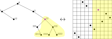
We denote with the youngest common ancestor of and namely is the largest vertex (for the order ) such that and for some We also denote by the fringe subtree of rooted at i.e., the subtree of containing all the vertices such that
Finally, we recall the following definition of a standard model for random trees.
Definition 3.2.
A -valued random variable is said to have the branching property if for conditionally on , the fringe subtrees, rooted at the children of the root, are independent and distributed as the original tree . A -valued random variable is a Galton–Watson tree with offspring distribution if it has the branching property and the distribution of is
3.2. Depth-first traversal
We now recall two classical ways of visiting the vertices of a rooted ordered tree that go under the name of depth-first traversal. These traversals originally developed for algorithms searching vertices in a tree, work as follows. Let be a rooted ordered tree with root .
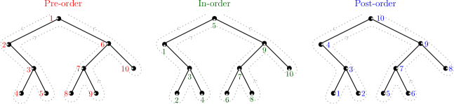
Definition 3.3 (Pre-order).
If consists only of , then is the pre-order traversal of . Otherwise, suppose that are the fringe subtrees in respectively rooted at the children of from left to right. The pre-order traversal begins by visiting . It continues by traversing in pre-order, then in pre-order, and so on, until is traversed in pre-order.
Definition 3.4 (Post-order).
If consists only of , then is the post-order traversal of . Otherwise, suppose that are the fringe subtrees in respectively rooted at the children of from left to right. The post-order traversal begins by traversing in post-order, then in post-order, and so on, until is traversed in post-order. It ends by visiting
We will also say that is labeled with the pre-order (resp. post-order) labeling starting from , if we associate the tag to the -th visited vertex by the pre-order (resp. post-order) traversal. Moreover, if we simply say that is labeled with the pre-order (resp. post-order), we will assume that we are starting from .
We will show an example in Fig. 8 in the case of binary trees.
3.3. Binary trees
We now introduce binary trees. We set
the set of finite binary words with the convention We use the same notation as in the case of ordered trees.
Definition 3.5.
A binary tree is a subset of that satisfies:
-
•
-
•
if then
Remark 3.6.
Note that a binary tree is not a particular rooted ordered tree. Indeed the third condition in Definition 3.1 is omitted in the case of binary trees. This implies that, if a vertex of a binary tree has only one child then it is either a left vertex (if it is marked with 1) or a right vertex (if it is marked with 2). See Fig. 7 for an example.
Given a vertex in the tree, we denote by and the left and the right fringe subtrees of hanging below the vertex We simply write and if namely, for the left and the right fringe subtrees below the root. Finally we let be the set of all binary trees.
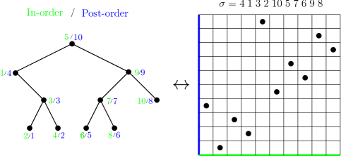
The notions of pre-order and post-order traversal extend immediately to binary trees. Moreover, in the case of binary trees, the in-order traversal is also available. Let be a binary tree with root .
Definition 3.7 (In-order).
If consists only of , then is the in-order traversal of . Otherwise the in-order traversal begins by traversing in in-order, then visits and concludes by traversing in in-order.
The notion of in-order labeling is defined similarly to the pre-order labeling or post-order labeling. We exhibit an example of the three different labelings in Fig. 8.
We finally extend the notion of Galton–Watson trees to binary Galton–Watson trees.
Definition 3.8.
A binary Galton–Watson tree with offspring distribution is a -valued random variable with the branching property and such that
4. The local limit for uniform random 231-avoiding permutations
The goal of this section is to prove that uniform random 231-avoiding permutations converge in the quenched Benjamini–Schramm sense. Before stating our precise result we fix some notation. Given a permutation we denote with LRMax() the set of indices of the left-to-right maxima of i.e., the values such that for every . Similarly we denote with RLMax() the set of indices of the right-to-left maxima of i.e., values such that for every Moreover, we set LRMax()CardLRMax() and RLMax()CardRLMax() We also fix and similarly we set Note that since contains only the index of the maximum of
For all we define the following probability distribution on
Remark 4.1.
Example 4.2.
We consider the permutation
where we draw in green the left-to-right maxima, in blue the right-to-left maxima, and in orange the maximum of the permutation, which is both a left-to-right maximum and a right-to-left maximum. We have LRMax() and RLMax() Thus
Before stating our main result, we recall the following trivial fact.
Observation 4.3.
If and then obviously Therefore, in what follow, we simply analyze the consecutive occurrences densities for
Theorem 4.4.
Let be a uniform random permutation in for all For all we have the following convergence in probability,
| (29) |
Since the limiting frequencies are deterministic, using Corollary 2.38, we have the following.
Corollary 4.5.
Let be a uniform random permutation in for all There exists a random infinite rooted permutation such that
Remark 4.6.
Section 4 is structured as follows:
-
•
in Section 4.1 we introduce a well-known bijection (see e.g., [16]) between binary trees and 231-avoiding permutations. Moreover we present a technique due to Janson [33]. With this tool we show that in order to study it is enough to study a similar expectation in terms of a specific binary Galton–Watson tree;
- •
- •
-
•
in Section 4.4 we give an explicit construction of the limiting object
4.1. Notation and preliminary results
4.1.1. Notation
We introduce some more notation. When convenient, we extend in the trivial way the various notation introduced for permutations to arbitrary sequences of distinct numbers. For example, we extend the notion of for two arbitrary sequences of distinct numbers and as
Given let indmax be the index of the maximal value i.e., If we set and respectively the (possibly empty) left and right subsequences of before and after the maximal value. In particular we have where we point out that is not the composition of permutations but just the concatenation of and seen as words.
We will write for namely, for the pattern occurring in the first positions of Similarly we will write for namely, for the pattern occurring in the last positions of Note that and stands for beginning and end. Moreover, if either or we set
To simplify notation, sometimes, if it is clear from the context, we will simply write or instead of or
We finally recall that a Laurent polynomial over is a linear combination of positive and negative powers of the variable with coefficients in i.e., of the form
where and for all We denote by an arbitrary Laurent polynomial in of valuation at least i.e., of the form Moreover we denote by a classical polynomial in of valuation at least i.e., of the form We remark that this is not the classical definition of since we are adding the additional hypothesis that the elements of are Laurent polynomials and not general functions.
4.1.2. A bijection between binary trees and 231-avoiding permutations
We present in this section a well-known bijection between 231-avoiding permutations and the set of binary trees (see e.g., [16]) which sends the size of the permutation to the number of vertices of the tree.
This bijection is based on the following result (see e.g., [15]).
Observation 4.7.
Let be a permutation and The permutation avoids if and only if and both avoid and furthermore whenever and
Given a permutation we build the following binary tree : if is empty then is the empty tree. Otherwise we add the root in which corresponds to the maximal element of and we split in and then the left subtree of will be the tree induced by i.e., and similarly, the right subtree of will be the tree induced by i.e.,
Conversely, given a binary tree we construct the corresponding permutation in as follows (cf. Fig. 9 below): if is empty then is the empty permutation. Otherwise we split in and and we set , the number of vertices of and Then we define as where is simply and is obtained by shifting all entries of by i.e., for all
It is clear that and are inverse of each other, hence providing the desired bijection.
From now until the end, we denote by the binary tree associated to and, analogously, by the permutation associated to the binary tree
Moreover, we define
and similarly
Observation 4.8.
By construction, the left-to-right maxima in a permutation correspond to the vertices in the left branch of , i.e., to the vertices of the form in the Neveu’s formalism. Similarly, the right-to-left maxima correspond to the vertices in the right branch of , i.e., to the vertices of the form Obviously the maximum corresponds to the root of the tree. An example is given in Fig. 10.
We make the following final remark that is not strictly necessary in this section but useful for comparison with the next one.
Remark 4.9.
It is not difficult to prove the following equivalent characterization of the bijection between trees and permutations based on the use of the tree traversals. Given a binary tree with vertices we reconstruct the corresponding permutation in setting to be equal to the label given by the post-order to the -th vertex visited by the in-order. Namely, we are using the in-order labeling for the indices of the permutation and the post-order labeling for the values. An example is provided in Fig. 11.
4.1.3. From uniform 231-avoiding permutations to binary Galton–Watson tree
Thanks to the bijection between binary trees and 231-avoiding permutations, instead of studying we can equivalently study the expectation where denotes a uniform random binary trees with vertices. A method for studying study the behavior of the latter expectation is to analyze the expectation for a binary Galton–Watson tree defined as follows.
For we set and we consider a binary Galton–Watson tree with offspring distribution defined by:
| (30) |
Remark 4.10.
Note that with this particular offspring distribution, having a left child is independent from having a right child.
We now state two lemmas due to Janson (see [33, Lemmas 5.2-5.4]). The first one is a result that rewrites the expectation of a function of in terms of uniform random binary trees with vertices using the classical fact that More precisely,
Lemma 4.11.
Let be a functional from the set of binary trees to such that for some constants and (this guarantees that all expectations and sums below converge). Then
where is the -th Catalan number.
Applying singularity analysis (see [24, Theorem VI.3]) one obtains:
Lemma 4.12.
If for where and then
Remark 4.13.
We recall that since by definition the elements of are Laurent polynomials (and not general functions) then they are –analytic in (for a precise definition see [24, Definition VI.1.]) and so the standard hypothesis to apply singularity analysis is fulfilled.
Lemma 4.12 shows us why it is enough to study the behavior of in order to derive information about the behavior of This will be the goal of the next section.
4.2. The annealed version of the Benjamini–Schramm convergence
In this section we are going to prove the following weaker version of Theorem 4.4.
Proposition 4.14.
Let be a uniform random permutation in for all It holds that
4.2.1. A basic recursion
Observation 4.7 gives us a basic recursion for as we will show in the next lemmas.
Lemma 4.15.
Let with Set Then, for any permutation with
| (31) |
where as always
Proof.
Recall that consecutive occurrences of in correspond to intervals such that We have three different possibilities for :
-
1.
if then is a consecutive occurrence in ;
-
2.
if then is a consecutive occurrence in ;
-
3.
if then has to be the interval Indeed and the value induced in by has to be
This is enough to prove Equation (31). ∎
We can translate this result in term of trees.
Lemma 4.16.
Let with and define as in the previous lemma. Then, for every binary tree denoting
| (32) |
4.2.2. The behaviour of .
We now focus on the behavior of for and then we will recover results for using Lemma 4.12 and the bijection between binary trees and 231-avoiding permutation as explained in Section 4.1.3. In order to simplify notation we set Thanks to Lemma 4.16, we know that, for all
| (33) |
where , and Taking the expectation in Equation (33) we obtain,
Since is an independent copy of with probability and empty with probability and the same holds for we have,
| (34) |
where in the last equality we used that We now focus on the term
Lemma 4.17.
Let Using notation as above and decomposing as usual in
| (35) |
Proof.
First of all note that
| (36) |
We recall that if (resp. ) is empty then (resp. ) is empty by definition.
We consider the case when We have,
since in Equation (36) the random tree is an independent copy of with probability and empty with probability and obviously the same hold also for The other three cases are similar. ∎
In view of Lemma 4.17, we now focus on (the analysis for following by symmetry). We want to rewrite the event conditioning on the position of the maximum among the last values of Using Observation 4.8, we know that this maximum is always reached at an index of corresponding to a vertex of of the form
with the convention For an example, see Fig. 12.
Therefore, defining the following events, for all all
and using the formula of total probability, we have
| (37) |
We also introduce the events, for all
Note that
| (38) |
The following lemma computes recursively and
Lemma 4.18.
Let Using notation as above,
| (39) |
and
| (40) |
Proof.
We start with the study of We distinguish again four different cases according to the structure of and .
-
•
By Equation (37), we know that
where in the last equality we used that conditioning on being the vertex in corresponding to the maximum among the last values of then Since the event is contained both in and in then
Using the independence between and conditionally on and continuing the sequence of equalities,
Since, conditionally on is an independent copy of with probability and empty with probability and the same obviously holds for we can rewrite the last term as
where in the last equality we used Equation (38).
-
•
Similarly as before
Noting that with similar arguments as before we have
and using again Equation (38), we can conclude that
-
•
Again
Noting that is empty by definition and using similar arguments as before, we have Therefore, using again Equation (38), we can write
-
•
Since then
Since the result for follows by symmetry, we can conclude the proof. ∎
We now continue the analysis of In order to do that, we need a formula for for a given tree because such probabilities appear in Equations (39) and (40).
Observation 4.19.
In a binary tree with vertices, every vertex has two potential children. Out of these potential children exist and do not exist. Hence
| (41) |
Using together Lemmas 4.17 and 4.18 and the above observation we have an explicit recursion to compute the probability We show an example of the recursion obtained for an explicit pattern .
Example 4.20.
Let be the following 231-avoiding permutation,
where, as before, we draw in green the left-to-right maxima, in blue the right-to-left maxima, and in orange the maximum.
We now make the explicit computation for using Lemmas 4.17 and 4.18. First of all, we recursively split our permutation as shown in Fig. 13.
Then, using Equation (35) with the decomposition of in (shown at the root of the tree in Fig. 13), we have
We continue decomposing and around their maxima (which correspond to the left and right children of the root in the tree in Fig. 13). Using Equation (39) for the left part, we obtain
and using Equation (40) for the right part, we obtain
where the first probability in the right-hand side is computed using Equation (41). Therefore, summing up the last three equations and then proceeding similarly through the left subtree in Fig. 13, we deduce that is the product of all the green factors in Fig. 13, that is
and this concludes Example 4.20.
We now proceed with the analysis of the general case. Using the recursion obtained by combining Lemmas 4.17 and 4.18 and Observation 4.19, we immediately realize that
| (42) |
Note that since in Lemmas 4.17 and 4.18 and Observation 4.19 the factors always appear with positive exponent. Moreover since in Equations (39) and (40), each time a factor appears, there is also a factor that contains a factor with
Since it follows that
We now compute the value In order to do that, we have to compute how many factors and appear in
Before stating our result we need to introduce a notion of distance between maxima. Given an index which is not the maximum of , we define its distance from the following left-to-right maximum as
Analogously, given an index which is not the maximum of , we define its distance from the following right-to-left maximum as
By convention, if is the index of the maximum of , then
Example 4.21.
We continue Example 4.2, where we considered the permutation
For LRMax() we have and for RLMax() we have and
We are now ready to state the key result of this section.
Proposition 4.22.
Let and be a Galton–Watson tree defined as above, then
| (43) |
Note that Proposition 4.22 claims that for the specific pattern given in Example 4.20 we have,
| (44) |
as previously computed. With this example in our hands, we can now use the same ideas in order to prove the proposition.
Proof of Proposition 4.22.
Suppose that we are able to prove that
| (45) |
Then noting that and that
we immediately derives the desired expression
We now prove Equation (45). As explained in the discussion below Equation (42), we just need to count how many factors and appear in the formula for . We can suppose that (if then the statement is trivial). Then by Equation (35),
| (46) |
and so we obtain either a factor (if the maximum of is reached at the first or at the last index of ) or a factor (otherwise). We recall that the asymptotics are for
We now look at the factors of the form By Equation (39),
| (47) |
We are going to focus on the factors that are not of the form We call them prefactors. For example, when and the prefactor is
Therefore, denoting by , we obtain:
-
(1)
for
-
•
if and then we have the following prefactor,
-
•
if (in this case ), then we have the following prefactor,
-
•
if (in this case ), then we have the following prefactor,
-
•
-
(2)
for i.e.,
-
•
in this case the index of the trivial maximum is and obviously hence we have the following prefactor,
-
•
Summing up, and noting that the analysis of the term is symmetric, we conclude that we have the following correspondence between maxima of and factor in the asymptotic expansion of
-
(a)
if is the index of the maximum of , by the comment below Equation (46), its contribution is
-
(b)
if and but is not the index of the maximum, by the previous analysis, its contribution is
-
(c)
if or but is not the index of the maximum, again by the previous analysis, its contribution is
Finally, we note that,
-
•
if or then
where the term 1 in the exponent comes from and the term comes from
-
•
if and then
where the term 2 in the exponent comes from and the term comes from
This proves Equation (45) and so it concludes the proof. ∎
Observation 4.23.
We can finally prove Proposition 4.14.
4.3. The quenched version of the Benjamini–Schramm convergence
In this section we finally prove Theorem 4.4. We are going to use a standard technique in probability theory called the Second moment method. We have to study the second moment As before we start with a result regarding trees and then we will extend it to permutations.
Proposition 4.24.
Using notation as before and setting we have,
Proof.
We use again the decomposition given by Lemma 4.16,
Taking the expectation of the square of the previous equation we obtain,
For the first two terms of the right-hand side of the above equation we use that is an independent copy of with probability and empty with probability (and similarly for ). Therefore we can rewrite the above expression as
| (49) |
where we have also used that We now analyze the four terms that appear on the right-hand side of the above equation.
First of all, using that is independent of we obtain
Applying Equation (48) and recalling that we conclude that
| (50) |
Obviously, using Proposition 4.22, we have
| (51) |
Therefore we have only to study the remaining two similar terms in Equation (49). Note that, if and using the same arguments that we already used in a lot of different steps, we have
Iterating the analysis of the second term (with similar techniques used in the proof of Lemma 4.18), we can conclude that is a Laurent polynomial in . Moreover, noting that we can obtain the following bound
By Equation (48), Therefore we can conclude that
| (52) |
Similarly,
| (53) |
Substituting Equations (50), (51), (52) and (53) in Equation (49), we finally have
We can finally prove our main theorem.
Proof of Theorem 4.4.
Applying again Lemma 4.12 and using our bijection between -avoiding permutations and binary trees, we conclude that for
| (54) |
This, with Proposition 4.14, implies that
| (55) |
We can apply the Second moment method and deduce that
Indeed by Chebyschev’s inequality, one has, for any fixed
and the right-hand side tends to zero. ∎
4.4. The construction of the limiting object
We now exhibit an explicit construction of the limiting object as a random order on
Remark 4.25.
The intuition behind the construction that we are going to present comes from the local limit for uniform binary trees (for more details, see [55]). When the size of a uniform binary tree tends to infinity, looking around a uniform distinguished vertex, we see an infinite upward spine. Each vertex in this spine is the left or the right child of the previous one with probability Moreover, attached to this infinite spine there are some independent copies of binary Galton–Watson trees. Using this idea and the bijection between binary trees and -avoiding permutations we are going to construct the limiting random total order.
This intuition is not formally needed in the following since we present the construction of the limiting object using the permutations point of view.
We have to introduce some notation. We define two operations from to for and ( is the set containing the empty permutation): let be a rooted permutation and be another (unrooted) permutation, we set
In words, from a graphical point of view, the diagram of (resp. ) is obtained starting from the diagram of the rooted permutation adding on the top-right (resp. bottom-left) the diagram of and adding a new maximal element between the two diagrams. We give an example below.
Example 4.26.
Let and then
Observation 4.27.
Note that, given a rooted permutation for all permutations (possibly empty), the rooted permutation (resp. ) contains at least one more element on the right (resp. left) of the root than .
We now consider two families of random variables: let be i.i.d. random variables with values in and Boltzman distribution equal to
This is a probability distribution since the generating function for the class is given by (see e.g., Appendix A). Moreover, let be i.i.d. random variables (also independent of ) with values in the set such that
Observation 4.28.
Recalling that is the binary Galton–Watson tree with offspring distribution defined by Equation (30), we note that, for
We are now ready to construct our random order on Set where is the random variable conditioned to be non empty, and is the (random) index of the maximum of Then we set,
Note that, for every fixed the sequence is a.s. stationary (hence a.s. convergent) by Observation 4.27 since asymptotically almost surely at least random variables are equal to and at least are equal to Let be the limit of this sequence. The family is a.s. consistent. Therefore, applying Proposition 2.12, the family determines a.s. a unique random total order such that, for all
Proposition 4.29.
Let be the random total order defined above and be the limiting object defined in Corollary 4.5. Then
Before proving the proposition we need to introduce some more notation in order to split a permutation in several different parts. In what follows, we suggest to compare the various definitions with the example in Fig. 14.
Given a pattern such that indmax and
with then we can decompose it as
| (56) |
| (57) |
where the different terms in the decomposition are precisely described in what follows.
We set,
where and We also set
i.e., in both cases, we are rooting at the index corresponding to the root of
Remark 4.30.
Note that, in general, if then i.e., the index of the maximum of does not correspond to the root of
Then, analyzing the left side of the pattern if we set
Finally, analyzing the right side of the pattern (regardless of being or not in ), if
we set
(with the convention that, if then ) and
(with the convention that, if then ).
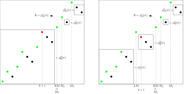
Proof of Proposition 4.29.
Since by Observation 2.23 the set of clopen balls
is a separating class for the space it is enough to prove that for all for all
| (58) |
We fix a pattern We first suppose that:
-
•
indmax
-
•
and with
-
•
is rooted at its maximum.
Using the notation explained before, rewrites as
Recalling that
and since by assumption is rooted at its maximum, by some easy combinatorial arguments, the event is equal to
where denotes the (random) index of the -th equal to (note that is almost surely well-defined). Using the independence of and we have,
Using Observation 4.23 and the fact that, for we have that,
Therefore, we can conclude that
This concludes the proof of Equation (58) when indmax and is rooted at its maximum. For the other cases we can proceed as follows:
-
•
if indmax but is not rooted at its maximum, we have to repeat the decomposition explained in Equations (56) and (57) for the permutation . We iterate this procedure until is rooted at its maximum (this procedure finishes since at each step ). In this way we obtain a new decomposition of Finally, with similar computations as before we can verify Equation (58);
-
•
if indmax then the proof of Equation (58) is similar to the one in the first case substituting the event with the event and then arguing exactly in the same way as before;
-
•
if indmax then Equation (58) follows from the previous cases by a symmetry argument;
- •
The analysis of all these cases concludes the proof. ∎
5. The local limit for uniform random 321-avoiding permutations
The goal of this section is to prove that uniform random 321-avoiding permutations converge in the quenched Benjamini–Schramm sense. We start by introducing, for all the following probability distribution on ,
| (59) |
Remark 5.1.
We note that the second condition (i.e., has exactly one descent, or equivalently, has exactly one inverse descent) is equivalent to saying that we can split the permutation in exactly two increasing subsequences such that all the values of one subsequence are smaller than the values of the other one. Formally, if and there exists a unique bipartition of as such that for all then and and are increasing.
Given the diagram of a permutation in with exactly one inverse descent, we call separating line the horizontal line in the diagram between these two increasing subsequences. An example is given in Fig. 15 in the case of the permutation where we highlight in orange the separating line between the two increasing subsequences.
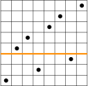
Remark 5.2.
That Equation (59) defines a probability distribution on is a consequence of Theorem 5.4 below: in Equation (60), summing over all the left-hand side, we obtain which trivially tends to 1. It is however easy to give a direct explanation. Indeed the number of permutations in with exactly one inverse descent and separating line at height is (where the binomial coefficient counts the possible choices of points that are below the separating line and the term stands for the identity permutation which has no inverse descent). Therefore the number of permutations in with exactly one inverse descent is
which entails
We now recall, similarly to the previous section, the following trivial fact.
Observation 5.3.
If and then obviously Therefore, in what follow, we simply analyze the consecutive occurrences densities for
Theorem 5.4.
Let be a uniform random permutation in for all We have the following convergence in probability,
| (60) |
Since the limiting frequencies are deterministic, using Corollary 2.38, we have the following.
Corollary 5.5.
Let be a uniform random permutation in for all There exists a random infinite rooted permutation such that
Remark 5.6.
The proof of Theorem 5.4 is structured as follows:
-
•
in Section 5.1 we introduce a well-known bijection between rooted ordered trees and 321-avoiding permutations. Moreover, we explain why it is enough to study a specific family of Galton–Watson trees;
- •
-
•
in Section 5.3 we introduce the notion of contour of a tree and we state some technical results about the characterization of the shape of some specific contours;
- •
-
•
finally, in Section 5.5 we give an explicit construction of the limiting object
5.1. From uniform 321-avoiding permutations to Galton–Watson trees
It is well known that 321-avoiding permutations can be broken into two increasing subsequences, one weakly above the diagonal and one strictly below the diagonal (see e.g., [17, Section 4.2]). Therefore, defining for every permutation
we have that and are the increasing patterns. Note that by convention the indices of fixed points are elements of
We now describe a slightly different, but equivalent (see Remark 5.8), version of a well-known bijection between 321-avoiding permutations (of size ) and rooted ordered trees (with vertices) – see e.g., [28].
We recall that denotes the set of rooted ordered trees with vertices (see Section 3 for notation about trees and random trees). Suppose has leaves and let be the list of leaves of listed in order of appearance in the pre-order traversal of i.e., from left to right. Moreover let and be the labels given to the leaf respectively by the pre-order labeling of starting from zero and the post-order labeling of starting from 1. We set and An example is given in the left-hand side of Fig. 16.
We start by constructing the permutation associated to the tree We define pointwise on as
and then we extend on by assigning values of in increasing order. Clearly is a -avoiding permutation. An example is given in Fig. 16.
We highlight (without proof, for more details see [28]) that this construction implies and It can also be proved that this construction is invertible: for a permutation there is a unique rooted ordered tree with vertices such that and
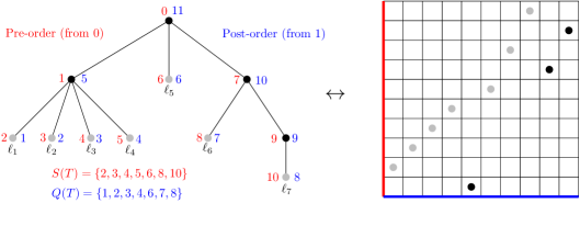
Observation 5.7.
Let i.e., for all We recall that a uniform random rooted ordered tree with vertices has the same distribution as a Galton–Watson tree with offspring distribution conditioned on having vertices (see [32, Example 9.1]), namely
| (61) |
Therefore, thanks to the bijection previously introduced, in order to prove Theorem 5.4, we can study a conditioned Galton–Watson tree instead of a uniform 321-avoiding permutation We also point out that a.s.
Remark 5.8.
At first sight, it seems that the construction presented here is different from that of [28], we argue here that they are in fact the same. In [28] the authors consider the same numbers but different numbers (denoted by in [28]) which are defined as follow
Note that Analyzing the difference between two consecutive values in we have
where we recall that is the first common ancestor of and We conclude that for all so our notation is consistent with that of [28].
5.2. A local limit result for Galton–Watson trees pointed at a uniform vertex
In this section we present a combination of two results due to Stufler [55] and Janson [32] that characterize the local limit for Galton–Watson trees pointed at a uniform vertex.
We begin by recalling the recent construction, due to Stufler, of the local limit tree We provide the construction in the special case where (cf. Fig. 17 below).
For each we let a vertex receive offspring according to an independent copy of , that is a random variable with size-biased distribution The vertex gets identified with a child of chosen uniformly at random. All other children of become the root of independent copies of the Galton–Watson tree Finally becomes the root of another independent copy of the Galton–Watson tree We always think of as a tree with distinguished vertex .
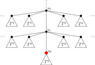
We point out that is not a tree in the classical Neveu’s formalism. We have to imagine that “the root” of the tree is at the end of the infinite backward spine composed by the vertices . Note also that has a.s. infinitely many vertices on the left and on the right of the infinite spine. For a formal construction of the set of these trees with infinite spine see [55, Section 4.1, p.6]. In what follows we will refer to this type of trees as trees with an infinite spine.
We now state the following easy reformulation of a result due to Janson [32]. First we recall that a rooted ordered tree together with a distinguished vertex is called a pointed rooted ordered tree and it is denoted by Given a pointed rooted ordered tree, we denote with the pointed fringe subtree rooted at the -th ancestor of the distinguished vertex (if this is not well-defined because has height smaller than , we set for some fixed placeholder value ). Similarly we denote with the fringe subtree of rooted at with distinguished vertex Despite is not a tree in Neveu’s formalism, is almost surely a pointed rooted ordered tree.
Finally, we denote with the set of pointed rooted ordered trees whose distinguished vertex has height .
Proposition 5.9.
Let be as before and be a uniform vertex of chosen independently of . Let also and Then
Proof.
Note that , for some can be rewritten as
where If we prove that, for all all
| (62) |
then the statement follows from the fact that is countable.
Note that
Indeed, if then Conversely, given such that there exists a unique choice for such that using the Neveu’s formalism, must be where is the pointed vertex of Therefore by [32, Theorem 7.12 (ii)], we have,
So, proving that will be enough to conclude the proof of Equation (62). This follows easily, since
and denoting with the path from the root to the parent of the distinguished vertex in
Remark 5.10.
Proposition 5.9 implies the local convergence of the rooted tree in the quenched sense, i.e., the convergence of the conditional random variable
5.3. Contour function for trees
In this section we recall the notion of contour function for trees and we generalize this definition for the local limit tree We start with the following.
Definition 5.11.
A Dyck path of length is a lattice path from to , consisting of up-steps (along the vector ) and down-steps (along the vector ), such that the path never goes below the -axis. We encode a Dyck path by a word containing letters and letters . The condition “the path never goes below the -axis” is equivalent to “every prefix contains at least as many ’s as ’s”.
Definition 5.12.
Given a rooted ordered tree with vertices, we define the contour of as the Dyck path of length obtained by turning around from left to right (as for the depth-first traversal), starting from the root, and recording, for each traversed edge, either an up-step if we are visiting the edge on the left from top to bottom or a down-step if we are visiting the edge on the right from bottom to top.
An example of contour of a tree is given in Fig. 18.
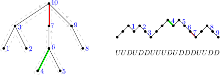
Remark 5.13.
From now until the end of Section 5, when we refer to labels, we always assume that we are speaking about labels given by the post-order labeling starting from 1. Moreover, given a rooted ordered tree and a label we use the abuse of notation for denoting the pointed tree with distinguished vertex labeled by Similarly, we will simply say “the vertex instead of “the vertex labeled by
We now make a connection between contours of trees and the labels of their leaves. We first introduce some notation for words over the alphabet We denotes by (resp. ) the set of finite words of length at least one composed only by letters (resp. ). Given two words , we write for the concatenation of the two words. More generally, given a family of words, we write for their consecutive concatenation.
Lemma 5.14.
Let (with ) be a set of labels. Then
Moreover, the shape of the contour of the tree between two consecutive leaves respectively labeled by is of the form
Proof.
Note that given a tree (cf. Fig. 18) and its contour then the leaves of correspond to letters in preceded by a . On the other hand, internal vertices (different from the root) correspond (for the first visit) to letters preceded by a and (for the last visit) to letters preceded by a . Therefore, given a tree such that the only down-steps in its contour preceded by an up-step are the first, and down-steps. Then it easily follows that The same reasoning also proves that given a tree such that
then concluding the proof. ∎
We now extend the notion of contour to the local limit tree We introduce some more notation for words over the alphabet We denote by the set of right-infinite words over the alphabet i.e., of infinite words of the form and similarly we denote by the set of left-infinite words over the alphabet i.e., of infinite words of the form
Definition 5.15.
A double-infinite pointed path is an infinite word in where
Definition 5.16.
The contour of a tree with an infinite spine is the double-infinite pointed path
obtained turning around the tree (cf. Fig. 19) in the following way:
-
•
we start the visit on the right of the vertex in the direction of the vertex (in Fig. 19 we start at the red square in the direction of the blue dashed line) and we set (i.e., is the down-step corresponding to the right-side of the edge between and );
-
•
we proceed turning around in the same direction (following the blue dashed line) setting, for all if the -th visited edge is visited from top to bottom, otherwise setting
-
•
we conclude coming back to the starting point (the red square) and turning around in the other direction (following the green dotted line), setting, for all if the -th visited edge is visited from bottom to top, otherwise setting
In particular, the contour of the local limit tree is the random double-infinite pointed path
obtained turning around the tree as explained before.
Observation 5.17.
Note that the contour of the local limit tree is consistent with the definition of contour on finite trees: the contour of a fringe subtree (forgetting the distinguished vertex) is a factor of (where has been replaced by ). Note also that contains at least up-steps and contains at least down-steps (corresponding to the edges for ).
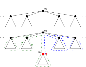
Lemma 5.18.
Let be the contour of Then is a sequence of i.i.d Bernoulli random variables on the set
Proof.
We fix Note that if and is the down-step corresponding to the right side of an edge in between the vertices and then:
-
•
if is the rightmost child of
-
•
if is not the rightmost child of
We claim that, conditioning on the event “ is the rightmost child of ” is independent of the shape of the contour of before the vertex namely is independent of Indeed, the number of children of each vertex of the tree is geometrically distributed (with parameter ) or size-biased geometrically distributed (with parameter ), and both distribution have the well-known memoryless property. This proves the claim. Moreover, thanks to this observation,
On the other hand, if and is the up-step corresponding to the left side of an edge in between the vertices and then:
-
•
if is a leaf;
-
•
if is not a leaf.
Note that cannot correspond to the left side of an edge in the infinite spine (since all these edges are visited on the right side when ), hence for all Moreover, we claim that, conditioning on the event “ is a leaf” is independent of the shape of the contour of before the vertex namely is independent of Indeed each vertex of the tree that is not in the infinite spine is a leaf with probability independently of all other vertices. This proves the claim.
Summing up, for all is a Bernoulli random variable independent of Using a symmetric argument for we can conclude the proof. ∎
5.4. The proof of the main result
We begin this section by stating two propositions that are the key results for the proof of Theorem 5.4. Then we prove Theorem 5.4 and at the end, in Sections 5.4.1 and 5.4.2, we give the proofs of the two propositions.
We need the following.
Definition 5.19.
Given a rooted ordered tree with vertices, we define for
i.e., is the set of values in shifted to the interval
Analogously, given a permutation we define for
Note that
Proposition 5.20.
For all let be a uniform random permutation in Fix and let be uniform in and independent of Then, for every subset as
Informally, conditionally on every index of is asymptotically equiprobably in or Moreover, these events are asymptotically independent.
Before stating our second proposition, we introduce some more notation (cf. Fig. 20 below). Given a permutation we define, for
with the conventions that and
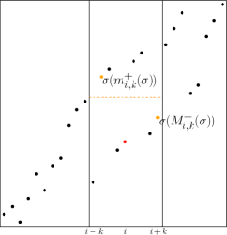
We also define, for a random 321-avoiding permutation and a uniform index the following events, for all
This is the event that the random rooted permutation splits into two (possibly empty) increasing subsequences with separated values, namely, the minimum of the upper subsequence is greater than the maximum of the lower subsequence. We will say, if this events holds, that “a separating line exists” (in Fig. 20 this separating line is dashed in orange).
Proposition 5.21.
For all let be a uniform random permutation in Fix and let be uniform in and independent of Then, as
Informally, conditionally on asymptotically almost surely there exists a separating line in .
With these two propositions in our hands, we can prove Theorem 5.4.
Proof of Theorem 5.4 .
In order to prove Equation (60) on page 60, we can check the equivalent condition (d) of Corollary 2.38, i.e., we have to prove that, for all for all
| (63) |
We fix and we distinguish three different cases for :
We recall (see Remark 5.1) that, in this case, splits in a unique way into two increasing subsequences whose indices are denoted by and Note that, in general, these two sets are different from and (specifically when the permutation has some fixed points at the beginning, for example as in the case of Fig. 15 on page 15). We set i.e., denotes the shifting of the set inside the interval Conditioning on namely assuming there is a separating line, is the union of two increasing subsequences with In particular, using Proposition 5.21, asymptotically we have that,
By Proposition 5.20 and 5.21, we have that
and so Equation (63) holds.
: In this case does not split in a unique way into two increasing subsequences. We have exacly different choices for this splitting, namely setting either or for some Therefore, using Proposition 5.21, asymptotically we obtain that
Again by Proposition 5.20 and 5.21, we have that
and so Equation (63) holds.
In this case does not present a separating line. Since by Proposition 5.21 we know that asymptotically almost surely there exists a separating line in we can immediately conclude that,
5.4.1. The proof of Proposition 5.20
We recall that denotes a Galton–Watson tree with offspring distribution conditioned on having vertices and is a uniform index in independent of the other random objects. We label the tree with the post-order labeling starting from 1 and, as said in Remark 5.13, we denote with the random pointed rooted ordered tree obtained from by distinguishing the vertex We also recall that .
Observation 5.22.
We need to introduce some technical results in order to study the event using Proposition 5.9. Informally, this event is not “local” in full generality, but it is “local” asymptotically almost surely.
Definition 5.23.
Given a tree we say that a vertex is before (resp. after) a vertex if the label of is smaller (resp. greater) than the label of
For all we consider the following events,
and
Lemma 5.24.
We have the following:
-
(a)
for all as
-
(b)
Proof.
(a) This is a trivial application of Proposition 5.9;
(b) The result it is an immediate consequence of the fact that the limiting tree has a.s. infinitely many vertices on the left and on the right of the infinite spine. ∎
We note that, for all conditioning on the event we can rewrite the event as
where is the set of all pointed rooted ordered trees with at least vertices before and vertices after the vertex such that Therefore, using Proposition 5.9, for all
| (64) |
Lemma 5.25.
With the same notation as above,
Proof.
Suppose that where for all and for all For all using the same ideas as in Lemma 5.14 on the right and left part of the contour of , the event rewrites as
where for all and for all (see Fig. 21 for a representation of this event).
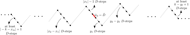
With these results in our hands we can finish the proof of Proposition 5.20.
Proof of Proposition 5.20.
We start studying the conditional probability which, we recall, is a random variable. For all almost surely,
Therefore, almost surely,
| (65) |
By Equation (64), for all the following limit for the lower bound in Equation (65) holds
| (66) |
Combining Equation (64) and Lemma 5.24 (a), for all the following limit for the upper bound in Equation (65) holds
| (67) |
Since the limiting objects are deterministic, the limits in Equations (66) and (67) hold jointly for all . Moreover, applying Skorokhod’s representation theorem in the product space over all we can also assume that there exists a coupling such that these limits hold also almost surely jointly for all . Therefore, almost surely, for all
| (68) |
Finally, since by Lemma 5.25,
and by Lemma 5.24 (a),
we can conclude, from Equation (68), that the limit in probability of exists and is equal to Finally, thanks to Observation 5.22,
5.4.2. The proof of Proposition 5.21
It remains to prove the following:
Before entering into the details, we first give a quick idea of the proof: by a result from [26], the points of a large uniform 321-avoiding permutation of size are at distance of order from the diagonal Therefore, in a window of constant width, the points above the diagonal are all higher than the points below the diagonal.
Proof of Proposition 5.21.
In order to simplify notation we fix and We split the probability into two different terms as follow,
We analyze the first term,
Setting for all we have
| (69) |
We now analyze the behavior of and By an easy application (stated in [35, p.10]) of a result due to Hoffman, Rizzolo and Slivken (see [26]) we can assume that there exist a coupling for where is a Brownian excursion, such that, almost surely,
where are error terms in probability of order uniformly in i.e., (w.r.t. the probability given by the coupling of ).
Therefore, setting or we obtain, almost surely,
where (w.r.t. the probability given by the coupling of ) since, almost surely, The same holds also for . In what follows all the probabilities and the error terms have to be interpreted in the same way, i.e. w.r.t. the probability given by the coupling of Moreover, we will simply denote the errors terms of order less than with
We can rewrite the last term in Equation (69) as
| (70) |
Noting that, if and , then a.s., we have that
Since is a continuous process, applying Lemma B.1 in the appendix, we can rewrite Equation (70) as
| (71) |
Noting that, if , than a.s., we can obtain the following bound,
| (72) |
From now until the end of the proof we denote with the family of random error terms that appears in the previous equation. Since where is a uniform random variable in by Skorokhod’s representation theorem, we can assume that the convergence holds almost surely. Since is a.s. continuous, we can deduce that
| (73) |
In particular, since and are independent ( is independent of hence of ), admits a density (called Rayleigh distribution, see [12, p.5]) and so the distribution function is continuous. From Equation (73), we can conclude that the convergence
is uniform in as stated in [13, exercise 14.8, p.198]. Therefore,
Finally, summing up, we obtain that
Noting that and using Markov’s inequality for the probability , we can conclude that,
5.5. The construction of the limiting object
We now exhibit an explicit construction of the limiting object as a random order on
We consider the set of integer numbers and we label, uniformly and independently, each integer with a “” or a “”: namely, for all
We set and Then we define a random total order on saying that, for all if either and or and or and An example is given in Fig. 22.
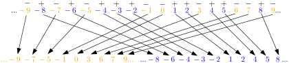
Proposition 5.26.
Let be the random total order defined above and be the limiting object defined in Corollary 5.5. Then
Proof.
Since by Observation 2.23 the set of clopen balls
is a separating class for the space it is enough to prove that for all for all
We fix and, as in the proof of Theorem 5.4, we distinguish three different cases for :
We recall (see Remark 5.1) that, in this case, splits in a unique way into two increasing subsequences whose indices are denoted by and Recalling that we have
: In this case does not split in a unique way into two increasing subsequences. We have exactly different choices for this splitting, namely setting either or for some Therefore, we obtain that
Since, by construction, contains a.s. at most one inverse descent, then
The analysis of this three cases concludes the proof. ∎
Appendix A A generating function proof that is a probability distribution
We give here a generating function proof of the fact that
| (74) |
defines a probability distribution on for all
Using our bijection between 231-avoiding permutations and binary trees, we can consider the generating function
where is the set of (possibly empty) binary trees. Using the classical decomposition of the binary trees in root, left subtree and right subtree, together with Observation 4.8, we obtain the following equation for our generating function,
| (75) |
where the term corresponds to the empty tree.
Now setting in Equation (75) and we obtain the classical relation for the generating function of Catalan numbers:
that can be algebraically solved to yield
Appendix B A small lemma
Lemma B.1.
Let be two sequences of real random variables with values in such that, for all
i.e., Then, for every real continuous random process (i.e., a random variable with values in ) we have
Proof.
Since is a.s. continuous on a compact set, it is also a.s. uniformly continuous. Therefore the continuity modulus tends a.s. to zero as tends to zero. By Skorokhod’s representation theorem we can assume that there exist a coupling such that therefore
Hence we can conclude that in the original probability space. ∎
Acknowledgements
The author is very grateful to Mathilde Bouvel and Valentin Féray for introducing him to the fantastic world of random permutations. He also thanks them for the constant and stimulating discussions and suggestions.
The author also warmly thanks Benedikt Stufler for precious suggestions about the terminology for Benjamini–Schramm convergence and for some explanations about local results for random trees.
Finally, he thanks Tommaso Padovan for precious help in the realization of various simulations and the anonymous referee for all his/her precious and useful comments.
This work was completed with the support of the SNF grant number , “Several aspects of the study of non-uniform random permutations”.
References
- [1] R. Abraham and J.-F. Delmas. An introduction to Galton-Watson trees and their local limits. ArXiv preprint:1506.05571, 2015.
- [2] D. Aldous. Asymptotic fringe distributions for general families of random trees. The Annals of Applied Probability, pages 228–266, 1991.
- [3] D. Aldous. The continuum random tree I. The Annals of Probability, pages 1–28, 1991.
- [4] D. Aldous. The continuum random tree II: an overview. Stochastic analysis, 167:23–70, 1991.
- [5] D. Aldous. The continuum random tree III. The Annals of Probability, pages 248–289, 1993.
- [6] D. Aldous and J. Pitman. Tree-valued Markov chains derived from Galton-Watson processes. In Annales de l’Institut Henri Poincare (B) Probability and Statistics, volume 34, pages 637–686. Elsevier, 1998.
- [7] D. Aldous and J. M. Steele. The objective method: probabilistic combinatorial optimization and local weak convergence. In Probability on discrete structures, pages 1–72. Springer, 2004.
- [8] O. Angel and O. Schramm. Uniform infinite planar triangulations. Communications in Mathematical Physics, 241(2-3):191–213, 2003.
- [9] F. Bassino, M. Bouvel, V. Féray, L. Gerin, M. Maazoun, and A. Pierrot. Universal limits of substitution-closed permutation classes. Journal of European Mathematical Society, to appear.
- [10] F. Bassino, M. Bouvel, V. Féray, L. Gerin, and A. Pierrot. The Brownian limit of separable permutations. The Annals of Probability, 46(4):2134–2189, 2018.
- [11] I. Benjamini and O. Schramm. Recurrence of distributional limits of finite planar graphs. Electronic Journal of Probability, 6, 2001.
- [12] J. Bertoin and J. Pitman. Path transformations connecting Brownian bridge, excursion and meander. Bulletin des sciences mathématiques, 118(2):147–166, 1994.
- [13] P. Billingsley. Probability and measure. John Wiley & Sons, 2008.
- [14] P. Billingsley. Convergence of probability measures. John Wiley & Sons, 2013.
- [15] M. Bóna. The absence of a pattern and the occurrences of another. Discrete Mathematics and Theoretical Computer Science, 12(2):89–102, 2010.
- [16] M. Bóna. Surprising symmetries in objects counted by Catalan numbers. the Electronic Journal of Combinatorics, 19(1):Paper 62, 11, 2012.
- [17] M. Bóna. Combinatorics of permutations. Chapman and Hall/CRC, 2016.
- [18] J. Borga, M. Bouvel, V. Féray, and B. Stufler. A decorated tree approach to random permutations in substitution-closed classes. ArXiv preprint:1904.07135, 2019.
- [19] J. Borga and E. Slivken. Square permutations are typically rectangular. ArXiv preprint:1904.03080, 2019.
- [20] A. Claesson and S. Kitaev. Classification of bijections between 321-and 132-avoiding permutations. Séminaire Lotharingien de Combinatoire, 60:B60d, 2008.
- [21] H. Crane, S. DeSalvo, and S. Elizalde. The probability of avoiding consecutive patterns in the Mallows distribution. Random Structures & Algorithms, 2018.
- [22] L. Devroye and S. Janson. Protected nodes and fringe subtrees in some random trees. Electronic Communications in Probability, 19, 2014.
- [23] S. Elizalde. A survey of consecutive patterns in permutations. In Recent trends in combinatorics, pages 601–618. Springer, 2016.
- [24] P. Flajolet and R. Sedgewick. Analytic combinatorics. Cambridge University press, 2009.
- [25] P. Frenkel. Convergence of graphs with intermediate density. Transactions of the American Mathematical Society, 370(5):3363–3404, 2018.
- [26] C. Hoffman, D. Rizzolo, and E. Slivken. Pattern-avoiding permutations and Brownian excursion part i: shapes and fluctuations. Random Structures & Algorithms, 50(3):394–419, 2017.
- [27] C. Hoffman, D. Rizzolo, and E. Slivken. Pattern-avoiding permutations and Brownian excursion, part ii: fixed points. Probability Theory and Related Fields, 169(1-2):377–424, 2017.
- [28] C. Hoffman, D. Rizzolo, and E. Slivken. Fixed points of 321-avoiding permutations. Proceedings of the American Mathematical Society, 147(2):861–872, 2019.
- [29] C. Holmgren and S. Janson. Fringe trees, Crump–Mode–Jagers branching processes and -ary search trees. Probability Surveys, 14:53–154, 2017.
- [30] C. Hoppen, Y. Kohayakawa, C. G. Moreira, B. Ráth, and R. M. Sampaio. Limits of permutation sequences. Journal of Combinatorial Theory, Series B, 103(1):93–113, 2013.
- [31] S. Janson. The Wiener index of simply generated random trees. Random Structures & Algorithms, 22(4):337–358, 2003.
- [32] S. Janson. Simply generated trees, conditioned Galton–Watson trees, random allocations and condensation. Probability Surveys, 9:103–252, 2012.
- [33] S. Janson. Patterns in random permutations avoiding the pattern 132. Combinatorics, Probability and Computing, 26(1):24–51, 2017.
- [34] S. Janson. Patterns in random permutations avoiding some sets of multiple patterns. ArXiv preprint:1804.06071, 2018.
- [35] S. Janson. Patterns in random permutations avoiding the pattern 321. Random Structures Algorithms,, 2018.
- [36] O. Kallenberg. Random measures, theory and applications. Springer, 2017.
- [37] R. Kenyon. Dominos and the Gaussian free field. Annals of probability, pages 1128–1137, 2001.
- [38] R. Kenyon, D. Kral, C. Radin, and P. Winkler. Permutations with fixed pattern densities. ArXiv preprint:1506.02340, 2015.
- [39] H. Kesten. Subdiffusive behavior of random walk on a random cluster. Ann. Inst. H. Poincaré Probab. Statist, 22(4):425–487, 1986.
- [40] M. Krikun. Local structure of random quadrangulations. ArXiv preprint: math/0512304, 2005.
- [41] J.-F. Le Gall. Uniqueness and universality of the Brownian map. The Annals of Probability, 41(4):2880–2960, 2013.
- [42] L. Lovász. Large networks and graph limits, volume 60. American Mathematical Soc., 2012.
- [43] M. Maazoun. On the Brownian separable permuton. ArXiv preprint:1711.08986, 2017.
- [44] N. Madras and L. Pehlivan. Structure of random 312-avoiding permutations. Random Structures & Algorithms, 49(3):599–631, 2016.
- [45] J.-F. Marckert and A. Mokkadem. Limit of normalized quadrangulations: the Brownian map. The Annals of Probability, 34(6):2144–2202, 2006.
- [46] G. Miermont. The Brownian map is the scaling limit of uniform random plane quadrangulations. Acta mathematica, 210(2):319–401, 2013.
- [47] S. Miner and I. Pak. The shape of random pattern-avoiding permutations. Advances in Applied Mathematics, 55:86–130, 2014.
- [48] J. Neveu. Arbres et processus de Galton-Watson. Annales de l’Institut Henri Poincaré. Probabilités et Statistique, 22(2):199–207, 1986.
- [49] R. Otter. The multiplicative process. The Annals of Mathematical Statistics, pages 206–224, 1949.
- [50] R. Pinsky. The infinite limit of random permutations avoiding patterns of length three. ArXiv preprint:1806.07669, 2018.
- [51] M. Rahman, B. Virag, and M. Vizer. Geometry of permutation limits. ArXiv preprint:1609.03891, 2016.
- [52] S. Sheffield. Gaussian free fields for mathematicians. Probability theory and related fields, 139(3-4):521–541, 2007.
- [53] S. Starr. Thermodynamic limit for the Mallows model on . Journal of mathematical physics, 50(9):095208, 2009.
- [54] R. Stephenson. Local convergence of large critical multi-type Galton–Watson trees and applications to random maps. Journal of Theoretical Probability, 31(1):159–205, 2018.
- [55] B. Stufler et al. Local limits of large galton–watson trees rerooted at a random vertex. In Annales de l’Institut Henri Poincaré, Probabilités et Statistiques, volume 55, pages 155–183. Institut Henri Poincaré, 2019.
- [56] V. Vatter. Permutation classes. In Handbook of enumerative combinatorics, Discrete Math. Appl. (Boca Raton), pages 753–833. CRC Press, Boca Raton, FL, 2015.