Approximate Leave-One-Out for Fast Parameter Tuning
in High Dimensions

Abstract

Consider the following class of learning schemes:

$$\hat{\bm{\beta}}:=\operatorname*{arg\,min}_{\bm{\beta}}\;\sum_{j=1}^{n}\ell({\bm{x}}_{j}^{\top}\bm{\beta};y_{j})+\lambda R(\bm{\beta}),$$ (1)

where ${\bm{x}}_{i}\in\mathbb{R}^{p}$ and $y_{i}\in\mathbb{R}$ denote the $i^{\rm th}$ feature and response variable respectively. Let $\ell$ and $R$ be the loss function and regularizer, $\bm{\beta}$ denote the unknown weights, and $\lambda$ be a regularization parameter. Finding the optimal choice of $\lambda$ is a challenging problem in high-dimensional regimes where both $n$ and $p$ are large. We propose two frameworks to obtain a computationally efficient approximation ALO of the leave-one-out cross validation (LOOCV) risk for nonsmooth losses and regularizers. Our two frameworks are based on the primal and dual formulations of (1). We prove the equivalence of the two approaches under smoothness conditions. This equivalence enables us to justify the accuracy of both methods under such conditions. We use our approaches to obtain a risk estimate for several standard problems, including generalized LASSO, nuclear norm regularization, and support vector machines. We empirically demonstrate the effectiveness of our results for non-differentiable cases.

1 Introduction

1.1 Motivation

Consider a standard prediction problem in which a dataset $\{(y_{j},{\bm{x}}_{j})\}_{j=1}^{n}\subset\mathbb{R}\times\mathbb{R}^{p}$ is employed to learn a model for inferring information about new datapoints that are yet to be observed. One of the most popular classes of learning schemes, specially in high-dimensional settings, studies the following optimization problem:

$$\hat{\bm{\beta}}:=\operatorname*{arg\,min}_{\bm{\beta}}\;\sum_{j=1}^{n}\ell({\bm{x}}_{j}^{\top}\bm{\beta};y_{j})+\lambda R(\bm{\beta}),$$ (2)

where $\ell:\mathbb{R}^{2}\rightarrow\mathbb{R}$ is the loss function, $R:\mathbb{R}^{p}\rightarrow\mathbb{R}$ is the regularizer, and $\lambda$ is the tuning parameter that specifies the amount of regularization. By applying an appropriate regularizer in (2), we are able to achieve better bias-variance trade-off and pursue special structures such as sparsity and low rank structure. However, the performance of such techniques hinges upon the selection of tuning parameters.

The most generally applicable tuning method is cross validation [38]. One common choice is $k$-fold cross validation, which however presents potential bias issues in high-dimensional settings where $n$ is comparable to $p$. For instance, the phase transition phenomena that happen in such regimes [3, 13, 14] indicate that any data splitting may cause dramatic effects on the solution of (2) (see Figure 1 for an example). Hence, the risk estimates obtained from $k$-fold cross validation may not be reliable. The bias issues of $k$-fold cross validation may be alleviated by choosing the number of folds $k$ to be large. However, such schemes are computationally demanding and may not be useful for emerging high-dimensional applications. An alternative choice of cross validation is LOOCV, which is unbiased in high-dimensional problems. However, the computation of LOOCV requires training the model $n$ times, which is unaffordable for large datasets.

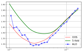
Figure 1: Risk estimates of LASSO based on 5-fold CV and ALO proposed in this paper, compared with the true out-of-sample prediction error (OOS). In this example, 5-fold CV provides biased estimates of OOS, while ALO works just fine. Here we use $n=5000$, $p=4000$ and $iid$ Gaussian design.

The high computational complexity of LOOCV has motivated researchers to propose computationally less demanding approximations of the quantity. Early examples offered approximations for the case $R(\bm{\beta})=\frac{1}{2}\|\bm{\beta}\|_{2}^{2}$ and the loss function being smooth [1, 32, 25, 9, 27, 31]. In [6], the authors considered such approximations for smooth loss functions and smooth regularizers. In this line of work, the accuracy of the approximations was either not studied or was only studied in the $n$ large, $p$ fixed regime. In a recent paper, [35] employed a similar approximation strategy to obtain approximate leave-one-out formulas for smooth loss functions and smooth regularizers. They show that under some mild conditions, such approximations are accurate in high-dimensional settings. Unfortunately, the approximations offered in [35] only cover twice differentiable loss functions and regularizers. On the other hand, numerous modern regularizers, such as generalized LASSO and nuclear norm, and also many loss functions are not smooth.

In this paper, we propose two powerful frameworks for calculating an approximate leave-one-out estimator (ALO) of the LOOCV risk that are capable of offering accurate parameter tuning even for non-differentiable losses and regularizers. Our first approach is based on the smoothing and quadratic approximation of the primal problem (2). The second approach is based on the approximation of the dual of (2). While the two approaches consider different approximations that happen in different domains, we will show that when both $\ell$ and $r$ are twice differentiable, the two frameworks produce the same ALO formulas, which are also the same as the formulas proposed in [35].

We use our platforms to obtain concise formulas for several popular examples including generalized LASSO, support vector machine (SVM) and nuclear norm minimization. As will be clear from our examples, despite of the equivalence of the two frameworks for smooth loss functions and regularizers, the technical aspects of the derivations involved for obtaining ALO formulas have major variations in different examples. Finally, we present extensive simulations to confirm the accuracy of our formulas on various important machine learning models. Code is available at github.com/wendazhou/alocv-package.

1.2 Other Related Work

The importance of parameter tuning in learning systems has encouraged many researchers to study this problem from different perspectives. In addition to cross validation, several other approaches have been proposed including Stein’s unbiased risk estimate (SURE), Akaike information criterion (AIC), and Mallow’s $C_{p}$. While AIC is designed for smooth parametric models, SURE has been extended to emerging optimization problems, such as generalized LASSO and nuclear norm minimization [8, 15, 42, 43, 46].

Unlike cross validation which approximates the out-of-sample prediction error, SURE, AIC, and $C_{p}$ offer estimates for in-sample prediction error [20]. This makes cross validation more appealing for many learning systems. Furthermore, unlike ALO, both SURE and $C_{p}$ only work on linear models (and not generalized linear models) and their unbiasedness is only guaranteed under the Gaussian model for the errors. There has been little success in extending SURE beyond this model [16].

Another class of parameter tuning schemes are based on approximate message passing framework [4, 29, 30]. As pointed out in [30], this approach is intuitively related to LOOCV. It offers consistent parameter tuning in high-dimensions [29], but the results strongly depend on the independence of the elements of ${\bm{X}}$.

1.3 Notation

Lowercase and uppercase bold letters denote vectors and matrices, respectively. For subsets $A\subset\{1,2,\ldots,n\}$ and $B\subset\{1,2,\ldots,p\}$ of indices and a matrix ${\bm{X}}$, let ${\bm{X}}_{A,\cdot}$ and ${\bm{X}}_{\cdot,{\bm{B}}}$ denote the submatrices that include only rows of ${\bm{X}}$ in $A$, and columns of ${\bm{X}}$ in $B$ respectively. Let $\{a_{i}\}_{i\in S}$ denote the vector whose components are $a_{i}$ for $i\in S$. We may omit $S$, in which case we consider all indices valid in the context. For a function $f:\mathbb{R}\rightarrow\mathbb{R}$, let $\dot{f}$, $\ddot{f}$ denote its 1^st and 2^nd derivatives. For a vector ${\bm{a}}$, we use $\mathrm{diag}[{\bm{a}}]$ to denote a diagonal matrix ${\bm{A}}$ with $A_{ii}=a_{i}$. Finally, let $\nabla R$ and $\nabla^{2}R$ denote the gradient and Hessian of a function $R:\mathbb{R}^{p}\rightarrow\mathbb{R}$.

2 Preliminaries

2.1 Problem Description

In this paper, we study the statistical learning models in form (2). For each value of $\lambda$, we evaluate the following LOOCV risk estimate with respect to some error function $d$:

$$\mathrm{loo}_{\lambda}:=\frac{1}{n}\sum_{i=1}^{n}d(y_{i},{\bm{x}}_{i}^{\top}\hat{\bm{\beta}}^{/i}),$$ (3)

where $\hat{\bm{\beta}}^{/i}$ is the solution of the leave-$i$-out problem

$$\hat{\bm{\beta}}^{/i}:=\operatorname*{arg\,min}_{\bm{\beta}}\;\sum_{j\neq i}\ell({\bm{x}}_{j}^{\top}\bm{\beta};y_{j})+\lambda R(\bm{\beta}).$$ (4)

Calculating (4) requires training the model $n$ times, which may be time-consuming in high-dimensions. As an alternative, we propose an estimator $\tilde{\bm{\beta}}^{/i}$ to approximate $\hat{\bm{\beta}}^{/i}$ based on the full-data estimator $\hat{\bm{\beta}}$ to reduce the computational complexity. We consider two frameworks for obtaining $\tilde{\bm{\beta}}^{/i}$, and denote the corresponding risk estimate by:

$$\mathrm{alo}_{\lambda}:=\frac{1}{n}\sum_{i=1}^{n}d(y_{i},{\bm{x}}_{i}^{\top}\tilde{\bm{\beta}}^{/i}).$$ (5)

The estimates we obtain will be called approximated leave-one-out (ALO) throughout the paper.

2.2 Primal and Dual Correspondence

The objective function of penalized regression problem with loss $\ell$ and regularizer $R$ is given by:

$$P(\bm{\beta}):=\sum_{j=1}^{n}\ell({\bm{x}}_{j}^{\top}\bm{\beta};y_{j})+R(\bm{\beta}).$$ (6)

Here and subsequently, we absorb the value of $\lambda$ into $R$ to simplify the notation. We also consider the Lagrangian dual problem, which can be written in the form:

$$\min_{{\bm{\theta}}\in\mathbb{R}^{n}}D(\bm{\theta}):=\sum_{j=1}^{n}\ell^{*}(-\theta_{j};y_{j})+R^{*}({\bm{X}}^{\top}\bm{\theta}),$$ (7)

where $\ell^{*}$ and $R^{*}$ denote the Fenchel conjugates of $\ell$ and $R$ respectively. See the derivation in Appendix A.

It is known that under mild conditions, (6) and (7) are equivalent [7]. In this case, we have the primal-dual correspondence relating the primal optimal $\hat{\bm{\beta}}$ and the dual optimal $\hat{\bm{\theta}}$:

$$\begin{gathered}\hat{\bm{\beta}}\in\partial R^{*}({\bm{X}}^{\top}\hat{{\bm{\theta}}}),\quad{\bm{X}}^{\top}\hat{{\bm{\theta}}}\in\partial R(\hat{\bm{\beta}}),\\ {\bm{x}}_{j}^{\top}\hat{\bm{\beta}}\in\partial\ell^{*}(-\hat{\theta}_{j};y_{j}),\quad-\hat{\theta}_{j}\in\partial\ell({\bm{x}}_{j}^{\top}\hat{\bm{\beta}};y_{j}),\end{gathered}$$ (8)

where $\partial f$ denotes the set of subgradients of a function $f$. Below we will use both primal and dual perspectives for approximating $\mathrm{loo}_{\lambda}$.

3 Approximation in the Dual Domain

3.1 The First Example: LASSO

Let us first start with a simple example that illustrates our dual method in deriving an approximate leave-one-out (ALO) formula for the standard LASSO. The LASSO estimator, first proposed in [39], can be formulated as the penalized regression framework in (6) by setting $\ell(\mu;y)=(\mu-y)^{2}/2$, and $R(\bm{\beta})=\lambda\|\bm{\beta}\|_{1}$.

We recall the general formulation of the dual for penalized regression problems (7), and note that in the case of the LASSO we have:

$$\ell^{*}(\theta_{i};y_{i})=\frac{1}{2}(\theta_{i}-y_{i})^{2},\\ \quad R^{*}(\bm{\beta})=\begin{cases}0&\text{ if }\|\bm{\beta}\|_{\infty}\leq\lambda,\\ +\infty&\text{ otherwise.}\end{cases}$$

In particular, we note that the solution of the dual problem (7) can be obtained from:

$$\hat{{\bm{\theta}}}=\Pi_{\Delta_{X}}({\bm{y}}).$$ (9)

Here $\Pi_{\Delta_{X}}$ denotes the projection onto $\Delta_{X}$, where $\Delta_{X}$ is the polytope given by:

$$\Delta_{X}=\{{\bm{\theta}}\in\mathbb{R}^{n}:\|{\bm{X}}^{\top}{\bm{\theta}}\|_{\infty}\leq\lambda\}.$$

Let us now consider the leave-$i$-out problem. Unfortunately, the dimension of the dual problem is reduced by 1 for the leave-$i$-out problem, making it difficult to leverage the information from the full-data solution to help approximate the leave-$i$-out solution. We propose to augment the leave-$i$-out problem with a virtual $i$^th observation which does not affect the result of the optimization, but restores the dimensionality of the problem.

More precisely, let ${\bm{y}}_{a}$ be the same as ${\bm{y}}$, except that its $i$^th coordinate is replaced by $\hat{y}^{/i}_{i}={\bm{x}}_{i}^{\top}\hat{\bm{\beta}}^{/i}$, the leave-$i$-out predicted value. We note that the leave-$i$-out solution $\hat{\bm{\beta}}^{/i}$ is also the solution for the following augmented problem:

$$\min_{\bm{\beta}\in\mathbb{R}^{p}}\sum_{j=1}^{n}\ell({\bm{x}}_{j}^{\top}\bm{\beta};y_{a,j})+R(\bm{\beta}).$$ (10)

Let $\hat{{\bm{\theta}}}^{/i}$ be the corresponding dual solution of (10). Then, by (9), we know that

$$\hat{{\bm{\theta}}}^{/i}=\Pi_{\Delta_{X}}({\bm{y}}_{a}).$$

Additionally, the primal-dual correspondence (8) gives that $\hat{{\bm{\theta}}}^{/i}={\bm{y}}_{a}-{\bm{X}}\hat{\bm{\beta}}^{/i}$, which is the residual in the augmented problem, and hence that $\hat{\theta}^{/i}_{i}=0$. These two features allow us to characterize the leave-$i$-out predicted value $\hat{y}^{/i}_{i}$, as satisfying:

$${\bm{e}}_{i}^{\top}\Pi_{\Delta_{X}}\big{(}{\bm{y}}-(y_{i}-\hat{y}^{/i}_{i}){\bm{e}}_{i}\big{)}=0,$$ (11)

where ${\bm{e}}_{i}$ denotes the $i$^th standard vector. Solving exactly for the above equation is in general a procedure that is computationally comparable to fitting the model, which may be expensive. However, we may attempt to obtain an approximate solution of (11) by linearizing the projection operator at the full data solution $\hat{{\bm{\theta}}}$, or equivalently performing a single Newton step to solve the leave-$i$-out problem from the full data solution. The approximate leave-$i$-out fitted value $\tilde{y}^{/i}_{i}$ is thus given by:

$$\tilde{y}^{/i}_{i}=y_{i}-\frac{\hat{\theta}_{i}}{J_{ii}},$$ (12)

where ${\bm{J}}$ denotes the Jacobian of the projection operator $\Pi_{\Delta_{X}}$ at the full data problem ${\bm{y}}$. Note that $\Delta_{X}$ is a polytope, and thus the projection onto $\Delta_{X}$ is almost everywhere locally affine [42]. Furthermore, it is straightforward to calculate the Jacobian of $\Pi_{\Delta_{X}}$. Let $E=\{j:|{\bm{X}}_{j}^{\top}\hat{{\bm{\theta}}}|=\lambda\}$ be the equicorrelation set (where ${\bm{X}}_{j}$ denotes the $j^{\text{th}}$ column of ${\bm{X}}$), then we have that the projection at the full data problem ${\bm{y}}$ is locally given by a projection onto the orthogonal complement of the span of ${\bm{X}}_{\cdot,E}$, thus giving ${\bm{J}}={\bm{I}}-{\bm{X}}_{\cdot,E}({\bm{X}}_{\cdot,E}^{\top}{\bm{X}}_{\cdot,E})^{-1}{\bm{X}}_{\cdot,E}^{\top}$. We can then obtain $\tilde{y}^{/i}$ by plugging ${\bm{J}}$ in (12). Finally, by replaceing ${\bm{x}}_{i}^{\top}\tilde{\bm{\beta}}^{/i}$ with $\tilde{y}^{/i}_{i}$ in (5) we obtain an estimate of the risk.

3.2 General Case

In this section we extend the dual approach outlined in Section 3.1 to more general loss functions and regularizers.

General regularizers

Let us first extend the dual approach to other regularizers, while the loss function remains $\ell(\mu,y)=(\mu-y)^{2}/2$. In this case the dual problem (7) has the following form:

$$\min_{{\bm{\theta}}}\frac{1}{2}\sum_{j=1}^{n}(\theta_{j}-y_{j})^{2}+R^{*}({\bm{X}}^{\top}{\bm{\theta}}).$$ (13)

We note that the optimal value of ${\bm{\theta}}$ is by definition the value of the proximal operator of $R^{*}({\bm{X}}^{\top}\cdot)$ at ${\bm{y}}$:

$$\hat{{\bm{\theta}}}=\bm{\mathrm{prox}}_{R^{*}({\bm{X}}^{\top}\cdot)}({\bm{y}}).$$

Following the argument of Section 3.1, we obtain

$$\tilde{y}^{/i}_{i}=y_{i}-\frac{\hat{\theta}_{i}}{J_{ii}},$$ (14)

with ${\bm{J}}$ now denoting the Jacobian of $\bm{\mathrm{prox}}_{R^{*}({\bm{X}}^{\top}\cdot)}$. We note that the Jacobian matrix ${\bm{J}}$ exists almost everywhere, because the non-expansiveness of the proximal operator guarantees its almost-everywhere differentiability [11]. In particular, if ${\bm{y}}$ has distribution which is absolutely continuous with respect to the Lebesgue measure, ${\bm{J}}$ exists with probability 1. This approach is particularly useful when $R$ is a norm, as its Fenchel conjugate is then the convex indicator of the unit ball of the dual norm, and the proximal operator reduces to a projection operator.

General smooth loss

Let us now assume we have a convex smooth loss in (6), such as those that appear in generalized linear models. As we are arguing from a second-order perspective by considering Newton’s method, we will attempt to expand the loss as a quadratic form around the full data solution. We will thus consider the approximate problem obtained by expanding $\ell^{*}$ around the dual optimal $\hat{{\bm{\theta}}}$:

$$\min_{{\bm{\theta}}}\frac{1}{2}\sum_{j=1}^{n}\ddot{\ell}^{*}(-\hat{\theta}_{j};y_{j})\Bigg{(}\theta_{j}-\hat{\theta}_{j}-\frac{\dot{\ell}^{*}(-\hat{\theta}_{j};y_{j})}{\ddot{\ell}^{*}(-\hat{\theta}_{j};y_{j})}\Bigg{)}^{2}+R^{*}({\bm{X}}^{\top}{\bm{\theta}}).$$ (15)

The constant term has been removed from (15) for simplicity. We note that we have reduced the problem to a problem with a weighted $\ell_{2}$ loss which may be further reduced to a simple $\ell_{2}$ problem by a change of variable and a rescaling of ${\bm{X}}$. Indeed, let ${\bm{K}}$ be the diagonal matrix such that $K_{jj}=\sqrt{\ddot{\ell}^{*}(-\hat{\theta}_{j};y_{j})}$, and note that we have: $\dot{\ell}^{*}(-\hat{\theta}_{j};y_{j})={\bm{x}}_{j}^{\top}\hat{\bm{\beta}}:=\hat{y}_{j}$ by the primal-dual correspondence (8). Consider the change of variable ${\bm{u}}={\bm{K}}{\bm{\theta}}$ to obtain:

$$\min_{{\bm{u}}}\frac{1}{2}\sum_{j=1}^{n}\left(u_{j}-\frac{\hat{\theta}_{j}\ddot{\ell}^{*}(-\hat{\theta}_{j};y_{j})+\hat{y}_{j}}{\sqrt{\ddot{\ell}^{*}(-\hat{\theta}_{j};y_{j})}}\right)^{2}+R^{*}({\bm{X}}^{\top}{\bm{K}}^{-1}{\bm{u}}).$$

We may thus reduce to the $\ell_{2}$ loss case in (13) with a modified ${\bm{X}}$ and ${\bm{y}}$:

$${\bm{X}}_{u}={\bm{K}}^{-1}{\bm{X}},\quad{\bm{y}}_{u}=\left\{\frac{\hat{\theta}_{j}\ddot{\ell}^{*}(-\hat{\theta}_{j};y_{j})+\hat{y}_{j}}{\sqrt{\ddot{\ell}^{*}(-\hat{\theta}_{j};y_{j})}}\right\}_{j}.$$ (16)

Similar to (14), the ALO formula in the case of general smooth loss can be obtained as $\tilde{y}_{i}^{/i}=K_{ii}\tilde{y}_{u,i}^{/i}$, with

$$\tilde{y}_{u,i}^{/i}=y_{u,i}-\frac{K_{ii}\hat{\theta}_{i}}{J_{ii}},$$ (17)

where ${\bm{J}}$ is the Jacobian of $\bm{\mathrm{prox}}_{R^{*}({\bm{X}}_{u}^{\top}\cdot)}$.

4 Approximation in the Primal Domain

4.1 Smooth Loss and Regularizer

To obtain $\mathrm{loo}_{\lambda}$ we need to solve

$$\hat{\bm{\beta}}^{/i}:=\operatorname*{arg\,min}_{\bm{\beta}}\;\sum_{j\neq i}\ell({\bm{x}}_{j}^{\top}\bm{\beta};y_{j})+R(\bm{\beta}).$$ (18)

Assuming $\hat{\bm{\beta}}^{/i}$ is close to $\hat{\bm{\beta}}$, we can take a Newton step from $\hat{\bm{\beta}}$ towards $\hat{\bm{\beta}}^{/i}$ to obtain its approximation $\tilde{\bm{\beta}}^{/i}$ as:

$$\tilde{\bm{\beta}}^{/i}=\hat{\bm{\beta}}+\Big{[}\sum_{j\neq i}{\bm{x}}_{j}{\bm{x}}_{j}^{\top}\ddot{\ell}({\bm{x}}_{j}^{\top}\hat{\bm{\beta}};y_{j})+\nabla^{2}R(\hat{\bm{\beta}})\Big{]}^{-1}{\bm{x}}_{i}\dot{\ell}({\bm{x}}_{i}^{\top}\hat{\bm{\beta}};y_{i}).$$ (19)

By employing the matrix inversion lemma [19] we obtain:

$${\bm{x}}_{i}^{\top}\tilde{\bm{\beta}}^{/i}={\bm{x}}_{i}^{\top}\hat{\bm{\beta}}+\frac{H_{ii}}{1-H_{ii}\ddot{\ell}({\bm{x}}_{i}^{\top}\hat{\bm{\beta}};y_{i})}\dot{\ell}({\bm{x}}_{i}^{\top}\hat{\bm{\beta}};y_{i}),$$ (20)

where

$${\bm{H}}={\bm{X}}[{\bm{X}}^{\top}\mathrm{diag}[\{\ddot{\ell}({\bm{x}}_{i}^{\top}\hat{\bm{\beta}};y_{i})\}_{i}]{\bm{X}}+\nabla^{2}R(\hat{\bm{\beta}})]^{-1}{\bm{X}}^{\top}.$$ (21)

This is the formula reported in [35]. By calculating $\hat{\bm{\beta}}$ and ${\bm{H}}$ in advance, we can cheaply approximate the leave-$i$-out prediction for all $i$ and efficiently evaluate the LOOCV risk. On the other hand, in order to use the above strategy, twice differentiability of both the loss and the regularizer is necessary in a neighborhood of $\hat{\bm{\beta}}$. However, this assumption is violated for many machine learning models including LASSO, Nuclear norm, and SVM. In the next two sections, we introduce a smoothing technique which lifts the scope of the above primal approach to nondifferentiable losses and regularizers.

4.2 Nonsmooth Loss and Smooth Regularizer

In this section we study the piecewise smooth loss functions and twice differentiable regularizers. Such problems arise in SVM [12] and robust regression [22]. Before proceeding further, we clarify our assumptions on the loss function.

Definition 4.1.

A singular point of a function is called $q$^th order, if at this point the function is $q$ times differentiable, but its $(q+1)$^th order derivative does not exist.

Below we assume the loss $\ell$ is piecewise twice differentiable with $k$ zero-order singularities $v_{1},\ldots,v_{k}\in\mathbb{R}$. The existence of singularities prohibits us from directly applying strategies in (19) and (20), where twice differentiability of $\ell$ and $R$ is necessary. A natural solution is to first smooth out the loss function $\ell$, then apply the framework in the previous section to the smoothed version and finally reduce the smoothness to recover the ALO formula for the original nonsmooth problem.

As the first step, consider the following smoothing idea:

$$\ell_{h}(\mu;y)=:\frac{1}{h}\int\ell(u;y)\phi((\mu-u)/h)du,$$

where $h>0$ is a fixed number and $\phi$ is a symmetric, infinitely many times differentiable function with the following properties:

Normalization: $\int\phi(w)dw=1$, $\phi(w)\geq 0$, $\phi(0)>0$;

Compact support: $\mathrm{supp}(\phi)=[-C,C]$ for some $C>0$.

Now plug in this smooth version $\ell_{h}$ into (18) to obtain the following formula from (19):

$$\tilde{\bm{\beta}}^{/i}_{h}:=\hat{\bm{\beta}}_{h}+\Big{[}\sum_{j\neq i}{\bm{x}}_{j}{\bm{x}}_{j}^{\top}\ddot{\ell}_{h}({\bm{x}}_{j}^{\top}\hat{\bm{\beta}}_{h};y_{j})+\nabla^{2}R(\hat{\bm{\beta}}_{h})\Big{]}^{-1}{\bm{x}}_{i}\dot{\ell}_{h}({\bm{x}}_{i}^{\top}\hat{\bm{\beta}}_{h};y_{i}).$$ (22)

where $\hat{\bm{\beta}}_{h}$ is the minimizer on the full data from loss $\ell_{h}$ and $R$. $\tilde{\bm{\beta}}^{/i}_{h}$ is a good approximation to the leave-$i$-out estimator $\hat{\bm{\beta}}^{/i}_{h}$ based on smoothed loss $\ell_{h}$.

Setting $h\rightarrow 0$, we have that $\ell_{h}(\mu,y)$ converges to $\ell(\mu,y)$ uniformly in the region of interest (see Appendix C.1 for the proof), implying that $\lim_{h\rightarrow 0}\tilde{\bm{\beta}}^{/i}_{h}$ serves as a good estimator of $\lim_{h\rightarrow 0}\hat{\bm{\beta}}^{/i}_{h}$, which is heuristically close to the true leave-$i$-out $\hat{\bm{\beta}}^{/i}$. Equation (22) can be simplified in the limit $h\rightarrow 0$. We define the sets of indices $V$ and $S$ for the samples at singularities and smooth parts respectively:

$$V :=\{j:{\bm{x}}_{j}^{\top}\hat{\bm{\beta}}=v_{t}\text{ for some }t\in\{1,\ldots,k\}\},$$

$$S :=\{1,\dotsc,n\}\setminus V.$$

We characterize the limit of ${\bm{x}}_{i}^{\top}\tilde{\bm{\beta}}^{/i}_{h}$ below.

Theorem 4.1.

Under some mild conditions, as $h\rightarrow 0$,

$${\bm{x}}_{i}^{\top}\tilde{\bm{\beta}}^{/i}_{h}\rightarrow{\bm{x}}_{i}^{\top}\hat{\bm{\beta}}+a_{i}g_{\ell,i},$$

where

$$a_{i} =\begin{cases}\frac{W_{ii}}{1-W_{ii}\ddot{\ell}({\bm{x}}_{i}^{\top}\hat{\bm{\beta}};y_{i})}&\text{ if }i\in S,\\ \frac{1}{[({\bm{X}}_{V\cdot}{\bm{Y}}^{-1}{\bm{X}}_{V\cdot}^{\top})^{-1}]_{ii}}&\text{ if }i\in V,\\ \end{cases}$$

$${\bm{Y}} =\nabla^{2}R(\hat{\bm{\beta}})+{\bm{X}}_{S\cdot}^{\top}\mathrm{diag}[\{\ddot{\ell}({\bm{x}}_{j}^{\top}\hat{\bm{\beta}})\}_{j\in S}]{\bm{X}}_{S\cdot},$$

$$W_{ii} ={\bm{x}}_{i}^{\top}{\bm{Y}}^{-1}{\bm{x}}_{i}-{\bm{x}}_{i}^{\top}{\bm{Y}}^{-1}{\bm{X}}_{V,\cdot}^{\top}({\bm{X}}_{V,\cdot}{\bm{Y}}^{-1}{\bm{X}}_{V,\cdot}^{\top})^{-1}{\bm{X}}_{V,\cdot}{\bm{Y}}^{-1}{\bm{x}}_{i}.$$

For $i\in S$, $g_{\ell,i}=\dot{\ell}({\bm{x}}_{i}^{\top}\hat{\bm{\beta}};y_{i})$, and for $i\in V$, we have:

$${\bm{g}}_{\ell,V}=({\bm{X}}_{V,\cdot}{\bm{X}}_{V,\cdot}^{\top})^{-1}{\bm{X}}_{V,\cdot}[\nabla R(\hat{\bm{\beta}})-\sum_{j\in S}{\bm{x}}_{j}\dot{\ell}({\bm{x}}_{j}^{\top}\hat{\bm{\beta}};y_{j})].$$

We can obtain the ALO estimate of prediction error by plugging ${\bm{x}}_{i}^{\top}\hat{\bm{\beta}}+a_{i}g_{\ell,i}$ instead of ${\bm{x}}_{i}^{\top}\tilde{\bm{\beta}}^{/i}$ in (5). The conditions and proof of Theorem 4.1 can be found in the Appendix C.3.

4.3 Nonsmooth Regularizer and Smooth Loss

The smoothing technique proposed in the last section can also handle many nonsmooth regularizers. In this section we focus on separable regularizers $R$, defined as $R(\bm{\beta})=\sum_{l=1}^{p}r(\beta_{l})$, where $r:\mathbb{R}\rightarrow\mathbb{R}$ is piecewise twice differentiable with finite number of zero-order singularities in $v_{1},\ldots,v_{k}\in\mathbb{R}$. (Examples on non-separable regularizers are studied in Section 6.) We further assume the loss function $\ell$ to be twice differentiable and denote by $A=\{l:\hat{\beta}_{l}\neq v_{t},\text{ for any }t\in\{1,\ldots,k\}\}$ the active set.

For the coordinates of $\hat{\bm{\beta}}$ that lie in $A$, our objective function, constrained to these coordinates, is locally twice differentiable. Hence we expect $\hat{\bm{\beta}}^{/i}_{A}$ to be well approximated by the ALO formula using only $\hat{\bm{\beta}}_{A}$. On the other hand, components not in $A$ are trapped at singularities. Thus as long as they are not on the boundary of being in or out of the singularities, we expect these locations of $\hat{\bm{\beta}}^{/i}$ to stay at the same values.

Technically, consider a similar smoothing scheme for $r$:

$$r_{h}(w)=\frac{1}{h}\int r(u)\phi((w-u)/h)du,$$

and let $R_{h}(\bm{\beta})=\sum_{l=1}^{p}r_{h}(\beta_{l})$. We then consider the ALO formula of Model (18) with regularizer $R_{h}$.

$$\tilde{\bm{\beta}}^{/i}_{h}:=\hat{\bm{\beta}}_{h}+\Big{[}\sum_{j\neq i}{\bm{x}}_{j}{\bm{x}}_{j}^{\top}\ddot{\ell}({\bm{x}}_{j}^{\top}\hat{\bm{\beta}}_{h};y_{j})+\nabla^{2}R_{h}(\hat{\bm{\beta}}_{h})\Big{]}^{-1}{\bm{x}}_{i}\dot{\ell}_{h}({\bm{x}}_{i}^{\top}\hat{\bm{\beta}}_{h};y_{i}).$$ (23)

Setting $h\rightarrow 0$, (23) reduces to a simplified formula which heuristically serves as a good approximation to the true leave-$i$-out estimator $\hat{\bm{\beta}}^{/i}$, stated as the following theorem:

Theorem 4.2.

Under some mild conditions, as $h\rightarrow 0$,

$${\bm{x}}_{i}^{\top}\tilde{\bm{\beta}}^{/i}_{h}\rightarrow{\bm{x}}_{i}^{\top}\hat{\bm{\beta}}+\frac{H_{ii}\dot{\ell}({\bm{x}}_{i}^{\top}\hat{\bm{\beta}};y_{i})}{1-H_{ii}\ddot{\ell}({\bm{x}}_{i}^{\top}\hat{\bm{\beta}};y_{i})},$$

with

$${\bm{H}}={\bm{X}}_{\cdot,A}[{\bm{X}}_{\cdot,A}^{\top}\mathrm{diag}[\{\ddot{\ell}({\bm{x}}_{i}^{\top}\hat{\bm{\beta}};y_{i})\}_{i}]{\bm{X}}_{\cdot,A}+\nabla^{2}R(\hat{\bm{\beta}}_{A})]^{-1}{\bm{X}}_{\cdot,A}^{\top}.$$

The conditions and proof of Theorem 4.2 can be found in the Appendix C.2.

Remark 4.1.

For nonsmooth problems, higher order singularities do not cause issues: the set of tuning values which cause $\hat{\beta}_{l}$ (for regularizer) or ${\bm{x}}_{j}^{\top}\hat{\bm{\beta}}$ (for loss) to fall at those higher order singularities has measure zero.

Remark 4.2.

For both nonsmooth losses and regularizers, we need to invert some matrices in the ALO formula. Although the invertibility does not seem guaranteed in the general formula, as we apply ALO to specific models, the structures of the loss and/or the regularizer ensures this invertibility. For example, for LASSO, we have that the size of the active set $|E|\leq\min(n,p)$.

Remark 4.3.

We note that the dual approach is typically powerful for models with smooth losses and norm-type regularizers, such as the SLOPE norm and the generalized LASSO. On the other hand, the primal approach is valuable for models with nonsmooth loss or when the Hessian of the regularizer is feasible to calculate. Such regularizers often exhibit some type of separability or symmetry, such as in the case of SVM or nuclear norm.

5 Equivalence Between Primal and Dual Methods

Although the primal and dual methods may be harder or easier to carry out depending on the specific problem at hand, one may wonder if they always obtain the same result. In this section, we outline a unifying view for both methods, and state an equivalence theorem.

As both the primal and dual methods are based on a first-order approximation strategy, we will study them not as approximate solutions to the leave-$i$-out problem, but will instead show that they are exact solutions to a surrogate leave-$i$-out problem. Indeed, recall that the leave-$i$-out problem is given by (4), which cannot be solved in closed form. However, we note that the solution does exist in closed form in the case where both $\ell$ and $R$ are quadratic functions.

We may thus consider the approximate leave-$i$-out problem, where both $\ell$ and $R$ have been replaced in the leave-$i$-out problem (4) by their quadratic expansion at the full data solution:

$$\min_{\bm{\beta}^{/i}}\sum_{j\neq i}\tilde{\ell}({\bm{x}}_{j}^{\top}\bm{\beta}^{/i};y_{j})+\tilde{R}(\bm{\beta}^{/i}).$$ (24)

When both $\ell$ and $R$ are twice differentiable at the full data solution, $\tilde{\ell}$ and $\tilde{R}$ can be taken to simply be their respective second order Taylor expansions at $\hat{\bm{\beta}}$. When $\ell$ or $R$ is not twice differentiable at the full data solution, we have seen that it is still possible to obtain an ALO estimator through the proximal map (in the case of the dual) or through smoothing arguments (in the case of the primal). The corresponding quadratic surrogates may then be formulated as partial quadratic functions, that is, convex quadratic functions restricted to an affine subspace. However, due to space limitations we only focus on twice differentiable losses and regularizers here.

The way we obtain $\tilde{\bm{\beta}}^{/i}$ in (19) indicates that the primal formula in (20) and (21) are the exact leave-$i$-out solution of the surrogate primal problem (24). On the other hand, we may also wish to consider the surrogate dual problem, by replacing $\ell^{*}$ and $R^{*}$ by their quadratic expansion at full data dual solution $\hat{{\bm{\theta}}}$ in the dual problem (7). One may possibly worry that the surrogate dual problem is then different from the dual of the surrogate primal problem (24). This does not happen, and we have the following theorem.

Theorem 5.1.

Let $\ell$ and $R$ be twice differentiable convex functions. Let $\tilde{\ell}$ and $\tilde{R}$ denote the quadratic surrogates of the loss and regularizer at the full data solution $\hat{\bm{\beta}}$, and let $\tilde{\ell}_{D}^{*}$ and $\tilde{R}_{D}^{*}$ denote the quadratic surrogates of the conjugate loss and regularizer at the dual full data solution $\hat{{\bm{\theta}}}$. We have that the following problems are equivalent (have the same minimizer):

$$\min_{{\bm{\theta}}}\sum_{j=1}^{n}\tilde{\ell}^{*}(-\theta_{j};y_{j})+\tilde{R}^{*}({\bm{X}}^{\top}{\bm{\theta}}),$$ (25)

$$\min_{{\bm{\theta}}}\sum_{j=1}^{n}\tilde{\ell}^{*}_{D}(-\theta_{j};y_{j})+\tilde{R}^{*}_{D}({\bm{X}}^{\top}{\bm{\theta}}).$$ (26)

Additionally, we note that the dual method described in Section 3 solves the surrogate dual problem (26).

Theorem 5.2.

Let ${\bm{X}}_{u}$, ${\bm{y}}_{u}$ be as in (16), and let $\tilde{y}^{/i}_{u,i}$ be the transformed ALO obtained in (17). Let $\tilde{{\bm{y}}}_{a}$ be the same as ${\bm{y}}_{u}$ except $\tilde{y}_{a,i}=\tilde{y}^{/i}_{u,i}$. Then $\tilde{{\bm{y}}}_{a}$ satisfies

$$[\bm{\mathrm{prox}}_{\tilde{g}}(\tilde{{\bm{y}}}_{a})]_{i}=0,$$ (27)

where $\tilde{g}({\bm{u}})=\tilde{R}^{*}({\bm{X}}_{u}^{\top}{\bm{u}})$ and $\tilde{R}$ denotes the quadratic surrogate of the regularizer.

In particular, $\tilde{y}^{/i}_{i}=K_{ii}\tilde{y}^{/i}_{u,i}$ is the exact leave-$i$-out predicted value for the surrogate problem described in Theorem 5.1.

We refer the reader to the Appendix B for the proofs. These two theorems imply that for twice differentiable losses and regularizers, the frameworks we laid out in Sections 3 and 4 lead to exactly the same ALO formulas. This equivalence theorem reflects the deep connections between the primal and dual optimization problem. The central property used by the proof is captured in the following lemma:

Lemma 5.1.

Let $f$ be a proper closed convex function, such that both $f$ and $f^{*}$ are twice differentiable. Then, we have for any ${\bm{x}}$ in the domain of $f$:

$$\nabla^{2}f^{*}(\nabla f({\bm{x}}))=[\nabla^{2}f({\bm{x}})]^{-1}.$$

By combining this lemma with the primal dual correspondence (8), we obtain a relation between the curvature of the primal and dual problems at the optimal value, ensuring that the approximation is consistent with the dual structure.

6 Applications

6.1 Generalized LASSO

The generalized LASSO [41] is a generalization of the LASSO problem which captures many applications such as the fused LASSO [40], $\ell_{1}$ trend filtering [23] and wavelet smoothing in a unified framework. The generalized LASSO problem corresponds to the following penalized regression problem:

$$\min_{\bm{\beta}}\frac{1}{2}\sum_{j=1}^{n}(y_{j}-{\bm{x}}_{j}^{\top}\bm{\beta})^{2}+\lambda\|{\bm{D}}\bm{\beta}\|_{1}.$$ (28)

where the regularizer is parameterized by a fixed matrix ${\bm{D}}\in\mathbb{R}^{m\times p}$ which captures the desired structure in the data. We note that the regularizer is a semi-norm, and hence we can formulate the dual problem as a projection. In fact, a dual formulation of (28) can be obtained as (see Appendix D):

$$\min_{{\bm{\theta}},{\bm{u}}}\frac{1}{2}\|{\bm{\theta}}-{\bm{y}}\|_{2}^{2},$$

$$\text{subject to: }\|{\bm{u}}\|_{\infty}\leq\lambda\text{ and }{\bm{X}}^{\top}{\bm{\theta}}={\bm{D}}^{\top}{\bm{u}}.$$

The dual optimal solution satisfies $\hat{{\bm{\theta}}}=\Pi_{\Delta_{X}}({\bm{y}})$, where $\Delta_{X}$ is the polytope given by:

$$\Delta_{X}=\{{\bm{\theta}}\in\mathbb{R}^{n}:\exists{\bm{u}},\|u\|_{\infty}\leq\lambda\text{ and }{\bm{X}}^{\top}{\bm{\theta}}={\bm{D}}^{\top}u\}.$$

The projection onto the polytope $C=\{{\bm{D}}^{\top}{\bm{u}}:\|{\bm{u}}\|_{\infty}\leq\lambda\}$ is given in [41] as locally being the projection onto the affine space orthogonal to the nullspace of ${\bm{D}}_{\cdot,-E}$, where $E=\{i:|\hat{u}_{i}|=\lambda\}$ and $-E=\{1,\dotsc,p\}\setminus E$. Since $\Delta_{X}=[{\bm{X}}^{\top}]^{-1}C$ is the inverse image of $C$ under the linear map given by ${\bm{X}}^{\top}$, the projection onto $\Delta_{X}$ is given locally by the projection onto the affine space normal to the space spanned by the columns of $[{\bm{X}}^{\top}]^{+}\mathrm{null}\,{\bm{D}}_{\cdot,-E}$, provided ${\bm{X}}$ has full column rank. Here, $[{\bm{X}}^{\top}]^{+}$ denotes the Moore-Penrose pseudoinverse of ${\bm{X}}^{\top}$. Finally, to obtain a spanning set of this space, we may consider ${\bm{A}}={\bm{X}}{\bm{B}}$, where ${\bm{B}}$ is a set of vectors spanning the nullspace of ${\bm{D}}_{\cdot,-E}$. This allows us to compute ${\bm{H}}={\bm{A}}{\bm{A}}^{+}$, the projection onto the normal space required to compute the ALO.

6.2 Nuclear Norm

Consider the following matrix sensing problem

$$\hat{{\bm{B}}}:=\operatorname*{arg\,min}_{{\bm{B}}}\frac{1}{2}\sum_{j=1}^{n}(y_{j}-\langle{\bm{X}}_{j},{\bm{B}}\rangle)^{2}+\lambda\|{\bm{B}}\|_{*},$$ (29)

with ${\bm{B}},{\bm{X}}_{j}\in\mathbb{R}^{p_{1}\times p_{2}}$. $\langle{\bm{X}},{\bm{B}}\rangle=\mathrm{trace}({\bm{X}}^{\top}{\bm{B}})$ denotes the inner product. We use $\|\cdot\|_{*}$ for nuclear norm, which is defined as the sum of the singular values of a matrix. The nuclear norm is a unitarily invariant function of the matrix [26]. Such functions are only indirectly related to the components of the matrix, making their analysis difficult even when they are smooth, and exacerbating the difficulties when they are non-smooth such as in the case of the nuclear norm. In particular, the smoothing framework described in Section 4.3 cannot be applied directly.

We are nonetheless able to leverage the specific structure of such functions to obtain the following theorem. Let $R$ be a smooth unitarily invariant matrix function, with:

$$R({\bm{B}})=\sum_{j=1}^{\min(p_{1},p_{2})}r(\sigma_{j}),$$

where $\sigma_{j}$ denotes the $j$^th singular value of ${\bm{B}}$. Consider the following matrix penalized regression problem:

$$\hat{{\bm{B}}}=\operatorname*{arg\,min}_{{\bm{B}}}\sum_{j=1}^{n}\ell(\langle{\bm{X}}_{j},{\bm{B}}\rangle;y_{j})+\lambda R({\bm{B}}).$$

Without loss of generality, below we assume $p_{1}\geq p_{2}$. Let $\hat{{\bm{B}}}=\hat{{\bm{U}}}\mathrm{diag}[\hat{\bm{\sigma}}]\hat{{\bm{V}}}^{\top}$ be the singular value decomposition (SVD) of the full data estimator $\hat{{\bm{B}}}$, where $\hat{{\bm{U}}}\in\mathbb{R}^{p_{1}\times p_{1}}$, $\hat{{\bm{V}}}\in\mathbb{R}^{p_{2}\times p_{2}}$. Let $\hat{{\bm{u}}}_{k}$, $\hat{{\bm{v}}}_{l}$ be the $k$^th and $l$^th column of $\hat{{\bm{U}}}$ and $\hat{{\bm{V}}}$ respectively. $\mathrm{diag}[\hat{\bm{\sigma}}]$ in this section is a $p_{1}\times p_{2}$ matrix with $\hat{\sigma}_{j}$ on the diagonal of its upper square sub-matrix and 0 elsewhere. In addition, we assume all the $\hat{\sigma}_{j}$’s are nonzero. We then have the following ALO formula:

$$\langle{\bm{X}}_{i},\tilde{{\bm{B}}}^{/i}\rangle=\langle{\bm{X}}_{i},\hat{{\bm{B}}}\rangle+\frac{H_{ii}\dot{\ell}(\langle{\bm{X}}_{i},\hat{{\bm{B}}}\rangle;y_{i})}{1-H_{ii}\ddot{\ell}(\langle{\bm{X}}_{i},\hat{{\bm{B}}}\rangle;y_{i})},$$

where

$${\bm{H}}=\bm{\mathcal{X}}[\bm{\mathcal{X}}^{\top}\mathrm{diag}[\{\ddot{\ell}(\langle{\bm{X}}_{j},{\bm{B}}\rangle;y_{j})\}_{j}]\bm{\mathcal{X}}+\lambda\bm{\mathcal{G}}]^{-1}\bm{\mathcal{X}}^{\top}.$$

Here $\bm{\mathcal{X}}$ is a $n\times p_{1}p_{2}$ matrix and $\bm{\mathcal{G}}$ is a symmetric square $p_{1}p_{2}\times p_{1}p_{2}$ matrix given by:

$$\bm{\mathcal{X}}_{j,kl} =\hat{{\bm{u}}}_{k}^{\top}{\bm{X}}_{j}\hat{{\bm{v}}}_{l},$$ (30)

$$\bm{\mathcal{G}}_{kl,st} =\begin{cases}\ddot{r}(\hat{\sigma}_{t})&s=t=k=l,\\ \frac{\hat{\sigma}_{s}\dot{r}(\hat{\sigma}_{s})-\hat{\sigma}_{t}\dot{r}(\hat{\sigma}_{t})}{\hat{\sigma}_{s}^{2}-\hat{\sigma}_{t}^{2}}&s\neq t,s\leq p_{2},(k,l)=(s,t),\\ -\frac{\hat{\sigma}_{s}\dot{r}(\hat{\sigma}_{t})-\hat{\sigma}_{t}\dot{r}(\hat{\sigma}_{s})}{\hat{\sigma}_{s}^{2}-\hat{\sigma}_{t}^{2}}&s\neq t,s\leq p_{2},(k,l)=(t,s),\\ \frac{\dot{r}(\hat{\sigma}_{t})}{\hat{\sigma}_{t}}&s\neq t,s>p_{2},(k,l)=(s,t),\\ 0&\text{otherwise.}\end{cases}$$

Note that the rows of $\bm{\mathcal{X}}$ and the index of $\bm{\mathcal{G}}$ are vectorized in a consistent way. The proof can be found in Appendix E.2. A nice property of this result is that the effect on singular values decouples from the original matrix, enabling us to apply our smoothing strategy in Section 4.3 to function $r(\sigma)$ when it is nonsmooth. This leads to the following theorem for nuclear norm. For more details on the derivation, please refer to Appendix E.3.

Theorem 6.1.

Consider the nuclear-norm penalized matrix regression problem (29), and let $\hat{{\bm{B}}}=\hat{{\bm{U}}}\mathrm{diag}[\hat{\bm{\sigma}}]\hat{{\bm{V}}}^{\top}$ be the SVD of the full data estimator $\hat{{\bm{B}}}$, with $\hat{{\bm{U}}}\in\mathbb{R}^{p_{1}\times p_{1}}$, $\hat{{\bm{V}}}\in\mathbb{R}^{p_{2}\times p_{2}}$. Let $m=\mathrm{rank}(\hat{{\bm{B}}})$ be the number of nonzero $\hat{\sigma}_{j}$’s for $\hat{{\bm{B}}}$. Let $\tilde{{\bm{B}}}^{/i}_{h}$ denote the approximate of $\hat{{\bm{B}}}^{/i}$ obtained from the smoothed problem. Then, as $h\rightarrow 0$

$$\langle{\bm{X}}_{i},\tilde{{\bm{B}}}^{/i}_{h}\rangle\rightarrow\langle{\bm{X}}_{i},\hat{{\bm{B}}}\rangle+\frac{H_{ii}}{1-H_{ii}}(\langle{\bm{X}}_{i},\hat{{\bm{B}}}\rangle-y_{i}),$$

where

$${\bm{H}}=\bm{\mathcal{X}}_{\cdot,E}[\bm{\mathcal{X}}_{\cdot,E}^{\top}\bm{\mathcal{X}}_{\cdot,E}+\lambda\bm{\mathcal{G}}]^{-1}\bm{\mathcal{X}}_{\cdot,E}^{\top},$$

with $\bm{\mathcal{X}}$ as defined in (30) and with $\bm{\mathcal{G}}\in\mathbb{R}^{(mp_{1}+mp_{2}-m^{2})\times(mp_{1}+mp_{2}-m^{2})}$ given by:

$$\bm{\mathcal{G}}_{kl,st}=\begin{cases}0&s=t=k=l\leq m,\\ \frac{1}{\hat{\sigma}_{s}+\hat{\sigma}_{t}}&1\leq s\neq t\leq m,(k,l)=(s,t),\\ \frac{1}{\hat{\sigma}_{s}}&1\leq s\leq m<t\leq p_{2},(k,l)=(s,t),\\ \frac{1}{\hat{\sigma}_{t}}&1\leq t\leq m<s\leq p_{1},(k,l)=(s,t),\\ -\frac{1}{\hat{\sigma}_{s}+\hat{\sigma}_{t}}&1\leq s\neq t\leq m,(k,l)=(t,s),\\ -\frac{g_{r}[\hat{\sigma}_{t}]}{\hat{\sigma}_{s}}&1\leq s\leq m<t\leq p_{2},(k,l)=(t,s),\\ -\frac{g_{r}[\hat{\sigma}_{s}]}{\hat{\sigma}_{t}}&1\leq t\leq m<s\leq p_{2},(k,l)=(t,s),\\ 0&\text{otherwise.}\end{cases}$$ (31)

where for $t>m$, $\hat{\sigma}_{t}=0$ and $g_{r}[\hat{\sigma}_{t}]$ is the corresponding subgradient at this singular value, which can be obtained through the SVD of $\frac{1}{\lambda}\sum_{j=1}^{n}(y_{j}-\langle{\bm{X}}_{j},\hat{{\bm{B}}}\rangle){\bm{X}}_{j}$. The set $E$ is then defined as:

$$E=\{(k,l):k\leq m\text{ or }l\leq m\}.$$

Note that the indices of $\bm{\mathcal{G}}$ and the index set $E$ are consistent.

6.3 Linear SVM

The linear SVM optimization can be written as

$$\operatorname*{arg\,min}_{\bm{\beta}}\sum_{j=1}^{n}(1-y_{j}{\bm{x}}_{j}^{\top}\bm{\beta})_{+}+\frac{\lambda}{2}\|\bm{\beta}\|_{2}^{2},$$

with $y_{j}\in\{-1,1\}$ and $(\cdot)_{+}=\max\{\cdot,0\}$. Note that this is a special instance of the problem we studied in Section 4.2. Here, $\ell(u;y_{j})=(1-y_{j}u)_{+}$ has only one zero order singularity at $y_{j}$. Using Theorem 4.1 and simplifying the expressions, we obtain the following ALO formula for SVM:

$${\bm{x}}_{i}^{\top}\tilde{\bm{\beta}}^{/i}={\bm{x}}_{i}^{\top}\hat{\bm{\beta}}+a_{i}g_{\ell,i},$$

where

$$a_{i}=\left\{\begin{array}[]{ll}\frac{1}{\lambda}{\bm{x}}_{i}^{\top}({\bm{I}}_{p}-{\bm{X}}_{V,\cdot}^{\top}({\bm{X}}_{V,\cdot}{\bm{X}}_{V,\cdot}^{\top})^{-1}{\bm{X}}_{V,\cdot}){\bm{x}}_{i}&i\in S,\\ \big{(}\lambda[({\bm{X}}_{V,\cdot}{\bm{X}}_{V,\cdot}^{\top})^{-1}]_{ii}\big{)}^{-1}&i\in V,\\ \end{array}\right.$$

and for $i\in S$, $g_{\ell,i}=-y_{i}$ if $y_{i}{\bm{x}}_{i}^{\top}\hat{\bm{\beta}}<1$, $g_{\ell,i}=0$ if $y_{i}{\bm{x}}_{i}^{\top}\hat{\bm{\beta}}>1$, and for $i\in V$

$${\bm{g}}_{\ell,V}=({\bm{X}}_{V,\cdot}{\bm{X}}_{V,\cdot}^{\top})^{-1}{\bm{X}}_{V,\cdot}[\lambda\hat{\bm{\beta}}+\sum_{j:y_{j}{\bm{x}}_{j}^{\top}\hat{\bm{\beta}}<1}y_{j}{\bm{x}}_{j}].$$

Recall that $V=\{j:{\bm{x}}_{j}^{\top}\hat{\bm{\beta}}=y_{j}\}$ and $S=[1,\ldots,n]\backslash V$.

7 Numerical Experiments

We illustrate the performance of ALO through three experiments. The first two compare the ALO risk estimate with that of LOOCV. The third experiment compares the computational complexity of ALO with that of LOOCV. We have also evaluated the performance of ALO on real-world datasets. Due to lack of space, these results are presented in Appendix F.2. For the first experiment (Figure 2a), we run ALO and LOOCV for the three models studied in Section 6 (using fused LASSO [40] as a special case of generalized LASSO) and compare their risk estimates under the settings $n>p$ and $n<p$ respectively. The full details of the experiments are provided in Appendix F.

For the second experiment (Figure 2b), we consider the risk estimates for LASSO from ALO and LOOCV under settings with model mis-specification, heavy-tail noise and correlated design. For all three cases, ALO approximates LOOCV well.

	svm	fused lasso	nuclear norm
$n>p$
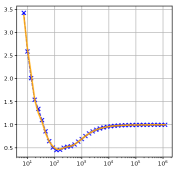
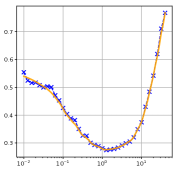
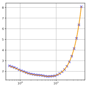
	$n=300,p=80$	$n=200,p=100$	$n=600,p_{1}=p_{2}=20$
$n<p$
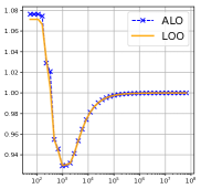
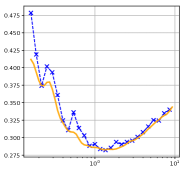
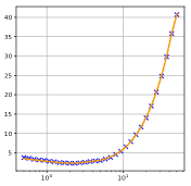
	$n=300,p=600$	$n=200,p=400$	$n=200,p_{1}=p_{2}=20$

(a)

	misspecification	heavy-tailed noise	correlated design
lasso risk

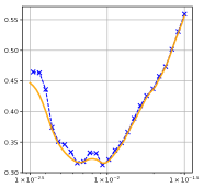
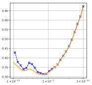
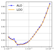
(b)

Figure 2: Risk estimates from ALO versus LOOCV. The $x$-axis is the tuning parameter value on $\log$-scale, the $y$-axis is the risk estimate. In part LABEL:sub@fg:experiment1, the comparison is based on SVM, fused LASSO and nuclear norm. Different settings for the number of observations $n$ and the number of features $p$ are considered. For nuclear norm, $p_{1},p_{2}$ are dimensions of a matrix. In part LABEL:sub@fg:experiment2, we consider the risk estimates of LASSO under model mis-specification, heavy-tailed noise and correlated design scenarios. We use $n=300$, $p=600$ and $k=30$ for all three where $k$ is the number of nonzeros in the true $\bm{\beta}$.

Table 1: Timing (in sec) of one single fit, ALO and LOOCV. In the upper and lower tables, we fix $n=800$ and $p=800$ respectively.

$p$	200	400	800	1600
single fit	$0.035\pm 0.001$	$0.13\pm 0.003$	$0.56\pm 0.02$	$0.60\pm 0.01$
ALO	$0.060\pm 0.001$	$0.21\pm 0.003$	$0.77\pm 0.02$	$0.89\pm 0.01$
LOOCV	$27.52\pm 0.03$	$107.4\pm 0.5$	$437.9\pm 2.9$	$479\pm 2$

$n$	200	400	800	1600
single fit	$0.055\pm 0.002$	$0.19\pm 0.006$	$0.56\pm 0.02$	$0.76\pm 0.02$
ALO	$0.065\pm 0.001$	$0.24\pm 0.001$	$0.77\pm 0.02$	$1.20\pm 0.01$
LOOCV	$11.44\pm 0.049$	$74.7\pm 0.5$	$437.9\pm 2.9$	$1249\pm 3$

In general, we observe that the estimates given by ALO are close to LOOCV, although the performance may deteriorate for very small values of $\lambda$, as is clear in the fused-LASSO ($n<p$) example. These values of $\lambda$ correspond to “dense” solutions, and are far from the optimal choice. Hence, such inaccuracies do not harm the parameter tuning algorithm.

Our last experiment compares the computational complexity of ALO with that of LOOCV. In Table 1, we provide the timing of LASSO for different values of $n$ and $p$. The time required by ALO, which involves a single fit and a matrix inversion (in the construction of ${\bm{H}}$ matrix), is in all experiments no more than twice that of a single fit. We refer the reader to Appendix F for the details of this experiment.

8 Discussion

ALO offers a highly efficient approach for parameter tuning and risk estimation for a large class of statistical machine learning models. We focus on nonsmooth models and propose two general frameworks for calculating ALO. One is from the primal perspective, the other from the dual.

By approximating LOOCV, ALO inherits desirable properties of LOOCV in high-dimensional settings where $n$ and $p$ are comparable. In particular, ALO can overcome the bias issues that $k$-fold cross validation displays in these settings.

Appendix A Proof of Equation 7

In this Section, we prove the primal-dual correspondence in (6) and (7). Recall the form of the primal problem:

$$\min_{\bm{\beta}}\sum_{j=1}^{n}\ell({\bm{x}}_{j}^{\top}\bm{\beta};y_{j})+R(\bm{\beta}).$$ (32)

With a change of variable, we may transform (32) into the following form:

$$\min_{\bm{\beta},\bm{\mu}}\sum_{j=1}^{n}\ell(-\mu_{j};y_{j})+R(\bm{\beta}),\quad\text{subject to: }\bm{\mu}=-{\bm{X}}\bm{\beta}.$$

We may further absorb the constraint into the objective function by adding a Lagrangian multiplier $\bm{\theta}\in\mathbb{R}^{n}$:

$$\max_{\bm{\theta}}\min_{\bm{\beta},\bm{\mu}}\sum_{j=1}^{n}\ell(-\mu_{j};y_{j})+R(\bm{\beta})-\bm{\theta}^{\top}({\bm{X}}\bm{\beta}+\bm{\mu}).$$ (33)

Note that in (33), $\bm{\beta}$ and $\bm{\mu}$ decoupled from each other and we can optimize over them respectively. Specifically, we have that

$$\min_{\bm{\beta}}R(\bm{\beta})-\bm{\theta}^{\top}{\bm{X}}\bm{\beta}=-\max_{\bm{\beta}}\big{\{}\langle\bm{\beta},{\bm{X}}^{\top}\bm{\theta}\rangle-R(\bm{\beta})\big{\}}=-R^{*}({\bm{X}}^{\top}\bm{\theta}),$$ (34)

$$\min_{\mu_{j}}\ell(-\mu_{j};y_{j})-\theta_{j}\mu_{j}=-\max\{\mu_{j}\theta_{j}-\ell(-\mu_{j};y_{j})\}=-\ell^{*}(-\theta_{j};y_{j}).$$ (35)

We plug (34) and (35) in (33) and obtain that

$$\max_{\bm{\theta}}\sum_{j=1}^{n}-\ell^{*}(-\theta_{j};y_{j})-R^{*}({\bm{X}}^{\top}\bm{\theta}).$$ (36)

Appendix B Primal Dual Equivalence (Proofs of Theorems 5.1 and 5.2)

In this section we prove the equivalence between the two stated methods in the case where the loss and regularizer are twice differentiable. Let $\ell$, $\ell^{*}$, $R$ and $R^{*}$ be twice differentiable. We construct quadratic surrogates by Taylor extensions. The following lemma plays a key role in our analysis:

Lemma B.1.

Let $f$ be a proper closed convex function, such that both $f$ and $f^{*}$ are twice differentiable. Then, we have for any ${\bm{x}}$ in the domain of $f$ and any ${\bm{u}}$ in the domain of $f^{*}$:

$$\nabla^{2}f^{*}(\nabla f({\bm{x}}))= [\nabla^{2}f({\bm{x}})]^{-1},$$

$$\nabla^{2}f(\nabla f^{*}({\bm{u}}))= [\nabla^{2}f^{*}({\bm{u}})]^{-1}.$$

Proof.

This lemma is a known result in convex optimization. However, since the proof is short and for the sake of completeness we include the proof here. For $f$ a proper closed convex function, we have by Theorem 23.5 of [36] that for all ${\bm{x}},{\bm{x}}^{*}$:

$${\bm{x}}^{*}\in\partial f({\bm{x}})\Rightarrow{\bm{x}}\in\partial f^{*}({\bm{x}}^{*}).$$

In particular, if $f$ and $f^{*}$ are differentiable, we obtain:

$${\bm{x}}=\nabla f^{*}(\nabla f({\bm{x}})).$$

Taking derivative in ${\bm{x}}$ once more, we obtain that:

$${\bm{I}}=[\nabla^{2}f^{*}(\nabla f({\bm{x}}))][\nabla^{2}f({\bm{x}})],$$

which immediately gives:

$$\nabla^{2}f^{*}(\nabla f({\bm{x}}))=[\nabla^{2}f({\bm{x}})]^{-1}.$$

The proof of the second part is immediate by applying the existing result to $f^{*}$. ∎

Proof of Theorem 5.1.

We have the following expressions for $\tilde{\ell}$ and $\tilde{R}$:

$$\tilde{\ell}(z_{j};y_{j})= \frac{1}{2}\ddot{\ell}({\bm{x}}_{j}^{\top}\hat{\bm{\beta}};y_{j})(z_{j}-{\bm{x}}_{j}^{\top}\hat{\bm{\beta}})^{2}+\dot{\ell}({\bm{x}}_{j}^{\top}\hat{\bm{\beta}};y_{j})(z_{j}-{\bm{x}}_{j}^{\top}\hat{\bm{\beta}})+c,$$

$$\tilde{R}(\bm{\beta})= \frac{1}{2}(\bm{\beta}-\hat{\bm{\beta}})^{\top}[\nabla^{2}R(\hat{\bm{\beta}})](\bm{\beta}-\hat{\bm{\beta}})+[\nabla R(\hat{\bm{\beta}})]^{\top}(\bm{\beta}-\hat{\bm{\beta}})+d,$$

where $c,d\in\mathbb{R}$ are constants that do not affect the location of the optimizer. We now compute the convex conjugate of $\tilde{\ell}$ and $\tilde{R}$, and we obtain that:

$$\tilde{\ell}^{*}(w_{j};y_{j})= \frac{1}{2}\frac{1}{\ddot{\ell}({\bm{x}}_{j}^{\top}\hat{\bm{\beta}};y_{j})}(w_{j}-\dot{\ell}({\bm{x}}_{j}^{\top}\hat{\bm{\beta}};y_{j}))^{2}+({\bm{x}}_{j}^{\top}\hat{\bm{\beta}})(w_{j}-\dot{\ell}({\bm{x}}_{j}^{\top}\hat{\bm{\beta}};y_{j}))+c^{\prime},$$ (37)

$$\tilde{R}^{*}(\bm{\mu})= \frac{1}{2}(\bm{\mu}-\nabla R(\hat{\bm{\beta}}))^{\top}[\nabla^{2}R(\hat{\bm{\beta}})]^{-1}(\bm{\mu}-\nabla R(\hat{\bm{\beta}}))+\hat{\bm{\beta}}^{\top}(\bm{\mu}-\nabla R(\hat{\bm{\beta}}))+d^{\prime},$$ (38)

where again $c^{\prime},d^{\prime}\in\mathbb{R}$ are constants.

Now, we wish to relate (37) and (38) to $\tilde{\ell}_{D}^{*}$ and $\tilde{R}_{D}^{*}$. By substituting the primal-dual correspondence described in (8) of the main text for components of (37) and (38), we obtain that:

$$\tilde{\ell}^{*}(w_{j};y_{j}) =\frac{1}{2}\frac{1}{\ddot{\ell}(\dot{\ell}^{*}(-\hat{\theta}_{j};y_{j});y_{j})}(w_{j}+\hat{\theta}_{j})^{2}+\dot{\ell}^{*}(-\hat{\theta}_{j};y_{j})(w_{j}+\hat{\theta}_{j})+c^{\prime},$$ (39)

$$\tilde{R}^{*}(\bm{\mu}) =\frac{1}{2}(\bm{\mu}-{\bm{X}}^{\top}\hat{{\bm{\theta}}})^{\top}[\nabla^{2}R(\nabla R^{*}({\bm{X}}^{\top}\hat{{\bm{\theta}}}))]^{-1}(\bm{\mu}-{\bm{X}}^{\top}\hat{{\bm{\theta}}})$$

$$\quad+[\nabla R^{*}({\bm{X}}^{\top}\hat{{\bm{\theta}}})]^{\top}(\bm{\mu}-{\bm{X}}^{\top}\hat{{\bm{\theta}}})+d^{\prime}.$$ (40)

To conclude, we note that according to Lemma B.1 we have

$$\begin{gathered}\ddot{\ell}(\dot{\ell}^{*}(-\hat{\theta}_{j};y_{j});y_{j})=(\ddot{\ell}^{*}(-\hat{\theta}_{j};y_{j}))^{-1},\\ \nabla^{2}R(\nabla R^{*}({\bm{X}}^{\top}\hat{{\bm{\theta}}}))=[\nabla^{2}R^{*}({\bm{X}}^{\top}\hat{{\bm{\theta}}})]^{-1}.\end{gathered}$$ (41)

Substitute (41) in (39) and (40) we obtain the dual of the quadratic surrogate equals

$$\frac{1}{2}\sum_{j}\tilde{\ell}^{*}(-\theta_{j};y_{j})+\tilde{R}^{*}({\bm{X}}^{\top}\theta) =\frac{1}{2}\sum_{j}\ddot{\ell}^{*}(-\hat{\theta}_{j};y_{j})\Big{(}-\theta_{j}+\hat{\theta}_{j}+\frac{\dot{\ell}^{*}(-\hat{\theta}_{j};y_{j})}{\ddot{\ell}^{*}(-\hat{\theta}_{j};y_{j})}\Big{)}^{2}$$

$$\quad+\frac{1}{2}({\bm{X}}^{\top}\bm{\theta}-{\bm{X}}^{\top}\hat{{\bm{\theta}}})\nabla^{2}R^{*}({\bm{X}}^{\top}\hat{{\bm{\theta}}})({\bm{X}}^{\top}\bm{\theta}-{\bm{X}}^{\top}\hat{{\bm{\theta}}})$$

$$\quad+[\nabla R^{*}({\bm{X}}^{\top}\hat{{\bm{\theta}}})]^{\top}({\bm{X}}^{\top}\bm{\theta}-{\bm{X}}^{\top}\hat{{\bm{\theta}}})+c^{\prime}.$$ (42)

We recognize that the formula given in (B) exactly corresponds to the second-order Taylor expansion of (15) in the main paper, which is just the form of $\tilde{\ell}_{D}^{*}$ and $\tilde{R}_{D}^{*}$. ∎

Additionally, we show that the augmented dual method solves the surrogate quadratic problem.

Proof of Theorem 5.2.

We noted in Section 3.2 of the main text that our dual method as described explicitly approximates the loss by its quadratic expansion at the optimal value. We may thus assume without loss of generality that the loss is given by $\ell(\mu;y)=(\mu-y)^{2}/2$.

In this case, as stated in Section 3.2, we have that

$$\hat{{\bm{\theta}}}=\bm{\mathrm{prox}}_{g}({\bm{y}}),$$

where we have defined $g({\bm{u}})=R^{*}({\bm{X}}^{\top}{\bm{u}})$. In addition, we note that the augmented observation vector ${\bm{y}}_{a}$ must have its $i$^th observation lie on the leave-$i$-out regression line by definition, and in particular we have that:

$$[\bm{\mathrm{prox}}_{g}({\bm{y}}_{a})]_{i}=0.$$

This motivated us to solve for $\tilde{y}_{i}^{/i}$ by linearly expanding $\bm{\mathrm{prox}}_{g}$ and considering the intersection of its $i$^th coordinate with 0. Specifically, the desired $\tilde{y}_{i}^{/i}$ is obtained from the solution of the following linear equation in $z$:

$$[\bm{\mathrm{prox}}_{g}({\bm{y}})+{\bm{J}}_{\bm{\mathrm{prox}}_{g}}({\bm{y}}){\bm{e}}_{i}(z-y_{i})]_{i}=0.$$ (43)

where ${\bm{J}}_{\bm{\mathrm{prox}}_{g}}({\bm{y}})$ denotes the Jacobian matrix of $\bm{\mathrm{prox}}_{g}$ at ${\bm{y}}$.

We show that if $R^{*}$ is replaced with its quadratic surrogate $\tilde{R}^{*}$ as defined in the Theorem 5.1, then:

$$[\bm{\mathrm{prox}}_{\tilde{g}}(\tilde{{\bm{y}}}_{a})]_{i}=0,$$

where $\tilde{g}({\bm{u}})=\tilde{R}^{*}({\bm{X}}^{\top}{\bm{u}})$, and $\tilde{{\bm{y}}}_{a}$ denotes the vector ${\bm{y}}$, except with its $i$^th coordinate replaced by the ALO value $\tilde{{\bm{y}}}^{/i}_{i}$. Let us note that as $\tilde{g}$ is quadratic, its proximal map $\bm{\mathrm{prox}}_{\tilde{g}}$ is linear, and the equation may thus be solved directly by a single Newton’s step. As a linear map is characterized by its intercept and slope, compared with (43), it remains to show that:

$$\bm{\mathrm{prox}}_{g}({\bm{y}}) =\bm{\mathrm{prox}}_{\tilde{g}}({\bm{y}}),$$ (44)

$${\bm{J}}_{\bm{\mathrm{prox}}_{g}}({\bm{y}}) ={\bm{J}}_{\bm{\mathrm{prox}}_{\tilde{g}}}({\bm{y}}).$$ (45)

We note that (44) is immediate from the definition of $\tilde{g}$, as both the left and right hand sides are equal to the dual optimal $\hat{{\bm{\theta}}}$. In order to show (45), since $\tilde{g}$ is quadratic, we may compute its proximal map exactly. From the previous section, we have that:

$$\tilde{g}({\bm{\theta}})=\frac{1}{2}(\bm{\theta}-\hat{{\bm{\theta}}})^{\top}{\bm{X}}[\nabla^{2}R(\nabla R^{*}({\bm{X}}^{\top}\hat{{\bm{\theta}}}))]^{-1}{\bm{X}}^{\top}(\bm{\theta}-\hat{{\bm{\theta}}})+[\nabla R^{*}({\bm{X}}^{\top}\hat{{\bm{\theta}}})]^{\top}{\bm{X}}^{\top}(\bm{\theta}-\hat{{\bm{\theta}}}),$$

We minimize $\frac{1}{2}\|{\bm{y}}-\bm{\theta}\|_{2}^{2}+\tilde{g}(\bm{\theta})$ in $\bm{\theta}$ and get

$$\bm{\mathrm{prox}}_{\tilde{g}}({\bm{y}})=({\bm{I}}+{\bm{X}}[\nabla^{2}R(\nabla R^{*}({\bm{X}}^{\top}\hat{\bm{\theta}}))]^{-1}{\bm{X}}^{\top})^{-1}({\bm{y}}-{\bm{X}}\nabla R^{*}({\bm{X}}^{\top}\hat{\bm{\theta}})),$$

Notice the primal dual correspondence implies $\hat{\bm{\beta}}=\nabla R^{*}({\bm{X}}^{\top}\hat{\bm{\theta}})$. In particular we may compute the Jacobian of $\bm{\mathrm{prox}}_{\tilde{g}}$ at ${\bm{y}}$ as $({\bm{I}}+{\bm{X}}[\nabla^{2}R(\hat{\bm{\beta}})]^{-1}{\bm{X}}^{\top})^{-1}$.

On the other hand, we know that the proximal operator $\bm{\mathrm{prox}}_{g}$ is exactly the resolvent of the subgradient $\partial g$:

$$\bm{\mathrm{prox}}_{g}=(I+\partial g)^{-1},$$

and in particular we have that:

$$\bm{\mathrm{prox}}_{g}({\bm{y}})+\nabla g(\bm{\mathrm{prox}}_{g}({\bm{y}}))={\bm{y}}.$$

Taking derivative again with respect to ${\bm{y}}$ and applying the chain rule, we obtain that:

$${\bm{J}}_{\bm{\mathrm{prox}}_{g}}({\bm{y}})({\bm{I}}+\nabla^{2}g(\bm{\mathrm{prox}}_{g}({\bm{y}})))={\bm{I}},$$

and hence that:

$${\bm{J}}_{\bm{\mathrm{prox}}_{g}}({\bm{y}})=({\bm{I}}+\nabla^{2}g(\bm{\mathrm{prox}}_{g}({\bm{y}}))^{-1}.$$

Now, note that we have $\bm{\mathrm{prox}}_{g}({\bm{y}})=\hat{{\bm{\theta}}}$, and that:

$$\nabla^{2}g(\hat{{\bm{\theta}}})={\bm{X}}[\nabla^{2}R^{*}({\bm{X}}^{\top}\hat{{\bm{\theta}}})]{\bm{X}}^{\top}.$$

We are thus done by Lemma B.1. ∎

Appendix C Proof of Primal Approximation Approach

In this section we prove the results of our primal approach on nonsmooth models presented in Section 4 of the main paper rigorously. Since we use a kernel smoothing strategy, we start with some useful preliminary results on kernel smoothing. We then discuss nonsmooth loss and nonsmooth regularizer respectively.

C.1 Properties of Kernel Smoothing

In the paper, we consider the following smoothing strategy for a convex function $f:\mathbb{R}\rightarrow\mathbb{R}$:

$$f_{h}(z)=\frac{1}{h}\int f(u)\phi((z-u)/h)du.$$ (46)

We make the following assumption about the kernel $\phi$:

Compact support: $\phi$ has a compact support, i.e., $\mathrm{supp}(\phi)=[-C,C]$ for some $C>0$;

Normalization: $\phi$ kernel: $\int\phi(w)dw=1$, $\phi(0)>0$; $\phi(x)\geq 0$ for every $x$;

Symmetry: $\phi$ is smooth and symmetric around 0 on $\mathbb{R}$.

Let $K:=\{v_{1},\ldots,v_{k}\}$ denote the set of zero-order singularities of the function $f$. Denote by $\dot{f}_{-}$ and $\dot{f}_{+}$ the left and right derivative of $f$. Our next lemma summarizes some of the basic properties of $f$ that may be used in the proofs of Theorem 4.1 and 4.2 of the main text.

Lemma C.1.

The smooth function $f_{h}$ verifies the following properties:

1. $f_{h}(z)\geq f(z)$ for all $z\in\mathbb{R}$;

2. For all $z\in K^{C}$, for all $h$ small enough:

   $$\dot{f}_{h}(z)=\frac{1}{h}\int\dot{f}(u)\phi((z-u)/h)du,\quad\ddot{f}_{h}(z)=\frac{1}{h}\int\ddot{f}(u)\phi((z-u)/h)du.$$

3. For all $z\in K$:

   $$\lim_{h\rightarrow 0}\dot{f}_{h}(z)=\frac{\dot{f}_{-}(z)+\dot{f}_{+}(z)}{2},\quad\lim_{h\rightarrow 0}\ddot{f}_{h}(z)=+\infty.$$

4. If $f$ is locally Lipschiz in the sense that, for any $A>0$, and for any $x,y\in[-A,A]$, we have $|f(x)-f(y)|\leq L_{A}|x-y|$, where $L_{A}$ is a constant that only depends on $A$; then $f_{h}(z)$ converges to $f(z)$ uniformly on any compact set.

Proof.

For part 1, by the normalization property of $\phi$, we can treat $\phi$ as a probability density. Consider the random variable $U\sim\frac{1}{h}\phi(\frac{z-u}{h})$. From the convexity of $f$ and Jensen’s inequality we have

$$f_{h}(z)=\mathbb{E}f(U)\geq f(\mathbb{E}U)=f(z).$$

For part 2, note that

$$\dot{f}_{h}(z)=\frac{1}{h^{2}}\int f(u)\dot{\phi}((z-u)/h)du=\int\dot{f}(u)\frac{1}{h}\phi((z-u)/h)du.$$

A similar computation gives the stated equation for $\ddot{f}_{h}(z)$.

For part 3, when $z\in K$, we have by compact support of $\phi$ that as $h\rightarrow 0$:

$$\dot{f}_{h}(z) =\frac{1}{h^{2}}\int_{z-hC}^{z}f(u)\dot{\phi}((z-u)/h)du+\frac{1}{h^{2}}\int_{z}^{z+hC}f(u)\dot{\phi}((z-u)/h)du$$

$$=\int_{-C}^{0}\dot{f}(z-hw)\phi(w)dw+\int_{0}^{C}\dot{f}(z-hw)\phi(w)dw$$

$$\rightarrow\int_{-C}^{0}\dot{f}_{+}(z)\phi(w)dw+\int_{0}^{C}\dot{f}_{-}(z)\phi(w)dw$$

$$=\frac{\dot{f}_{+}(z)+\dot{f}_{-}(z)}{2}.$$

A similar computation for the second-order derivative yields:

$$\ddot{f}_{h}(z) =\frac{1}{h^{3}}\int_{z-hC}^{z}f(u)\ddot{\phi}((z-u)/h)du+\frac{1}{h^{3}}\int_{z}^{z+hC}f(u)\ddot{\phi}((z-u)/h)du$$

$$=\frac{1}{h}\phi(0)(\dot{f}_{+}(z)-\dot{f}_{-}(z))+\int_{0}^{C}\ddot{f}(z-hw)\phi(w)dw+\int_{-C}^{0}\ddot{f}(z-hw)\phi(w)dw$$

$$\rightarrow\infty.$$

noticing that $\dot{f}_{+}(z)>\dot{f}_{-}(z)$.

For part 4, for any compact set $\mathcal{C}$ which can be covered by a large enough set $[-A,A]$ for some $A>0$, we have

$$\sup_{z\in\mathcal{C}}|f_{h}(z)-f(z)|\leq\sup_{z\in\mathcal{C}}\int_{-C}^{C}|f(z-hw)-f(z)|\phi(w)dw\leq 2hCL_{A+C}\rightarrow 0,\quad\text{ as }h\rightarrow 0$$

∎

Having established the basic properties of our kernel smoothing strategy, we apply them to non-smooth loss and non-smooth regularizer respectively.

C.2 Proof of Theorem 4.2: Nonsmooth Separable Regularizer With Smooth Loss

Consider the penalized regression problem:

$$\hat{\bm{\beta}}=\operatorname*{arg\,min}_{\bm{\beta}}\sum_{j=1}^{n}\ell({\bm{x}}_{j}^{\top}\bm{\beta};y_{j})+\lambda\sum_{l}r(\beta_{l}).$$ (47)

with $\ell$ and $r$ being twice differentiable and nonsmooth functions respectively. Let $r_{h}$ be the smoothed version of $r$ constructed as in (46). Define

$$\hat{\bm{\beta}}_{h}=\arg\min_{\bm{\beta}}\sum_{j}\ell({\bm{x}}_{j}^{\top}\bm{\beta};y_{j})+\lambda\sum_{l}r_{h}(\beta_{l}).$$

As before, let $K$ denote the set of all zero-order singularities of $r$. We make the following assumptions on the regularizer.

Assumption C.1.

We will need the following assumptions on the problem.

1. $r$ is locally Lipschiz in the sense that, for any $A>0$, and for any $x,y\in[-A,A]$, we have $|r(x)-r(y)|\leq L_{A}|x-y|$, where $L_{A}$ is a constant that only depends on $A$;

2. $\hat{\bm{\beta}}$ is the unique minimizer of (47);

3. When $\hat{\beta}_{l}=v\in K$, the subgradient $g_{r}(\hat{\beta}_{l})$ of $r$ at $\hat{\beta}_{l}$ satisfies $g_{r}(\hat{\beta}_{l})\in(\dot{r}_{-}(v),\dot{r}_{+}(v))$.

4. $r$ is coercive in the sense that $|r(z)|\rightarrow\infty$ as $|z|\rightarrow\infty$.
   

Lemma C.2.

Suppose that Assumption C.1 holds. There exists $M>0$ that only depends on $r,\ell$ and $\lambda$, such that we have for any $h\leq 1$:

$$\|\hat{\bm{\beta}}\|_{\infty},\|\hat{\bm{\beta}}_{h}\|_{\infty}<M.$$

Proof.

Let $h\leq 1$, then the minimizer of the smoothed version $\hat{\bm{\beta}}_{h}$ satifies

$$\lambda\sum_{l=1}^{p}r([\hat{\bm{\beta}}_{h}]_{l}) \leq\lambda\sum_{l=1}^{p}r_{h}([\hat{\bm{\beta}}_{h}]_{l})$$

$$\leq\sum_{i}\ell(y_{i};0)+\lambda pr_{h}(0)$$

$$=\sum_{i}\ell(y_{i};0)+\lambda p\int_{-C}^{C}r(hw)\phi(w)dw$$

$$\leq\sum_{i}\ell(y_{i};0)+\lambda p\sup_{|w|\leq C}r(w).$$

On the other hand, the minimizer $\hat{\bm{\beta}}$ of the original problem satisfies

$$\lambda\sum_{l=1}^{p}r([\hat{\bm{\beta}}]_{l})\leq\sum_{i}\ell(y_{i};0)+\lambda pr(0)\leq\sum_{i}\ell(y_{i};0)+\lambda p\sup_{|w|\leq C}r(w).$$

The convexity and coerciveness of $r$ implies that there exists an $M$, such that for all $h\leq 1$:

$$\|\hat{\bm{\beta}}_{h}\|_{\infty}\leq M\text{ and }\|\hat{\bm{\beta}}\|_{\infty}\leq M.$$

∎

Lemma C.3.

Suppose that Assumption C.1 holds. Then the smoothed version converges to the original problem in the sense that:

$$\|\hat{\bm{\beta}}_{h}-\hat{\bm{\beta}}\|_{2}\rightarrow 0\text{ as }h\rightarrow 0.$$

Proof.

By the local Lipschitz condition of $r$, we have for any $z\leq M$ and $h\leq 1$:

$$0\leq r_{h}(z)-r(z)=\int_{-C}^{C}[r(z-hw)-r(z)]\phi(w)dw\leq 2CL_{M+C}h.$$ (48)

Let $P_{h}(\bm{\beta}):=\sum_{j}\ell({\bm{x}}_{j}^{\top}\bm{\beta};y_{j})+\lambda\sum_{l}r_{h}(\beta_{l})$ denote the primal objective value. (48) implies that:

$$\sup_{\|\bm{\beta}\|_{\infty}\leq M}|P(\bm{\beta})-P_{h}(\bm{\beta})|\leq 2hpCL_{M+C}$$

By Lemma C.2 $\hat{\bm{\beta}}_{h}$ is in a compact set. Hence, any of its subsequence contains a convergent sub-subsequence. Let us abuse the notation and denote by $\hat{\bm{\beta}}_{h}$ any of such convergent sub-subsquence, that is, assume that $\hat{\bm{\beta}}_{h}\rightarrow\hat{\bm{\beta}}_{0}$. Along such a sub-subsequence, we have that:

$$P(\hat{\bm{\beta}}_{0})=\lim_{h\rightarrow 0}P(\hat{\bm{\beta}}_{h})=\lim_{h\rightarrow 0}P_{h}(\hat{\bm{\beta}}_{h})\leq\lim_{h\rightarrow 0}P_{h}(\hat{\bm{\beta}})=\lim_{h\rightarrow 0}P(\hat{\bm{\beta}}).$$

The uniqueness of the minimizer implies $\hat{\bm{\beta}}_{0}=\hat{\bm{\beta}}$. As the above holds along any convergent sub-subsequence, we have that:

$$\|\hat{\bm{\beta}}_{h}-\hat{\bm{\beta}}\|_{2}\rightarrow 0\text{ as }h\rightarrow 0.$$

∎

Lemma C.4 (Convergence of the subgradients).

Suppose that Assumption C.1 holds. Recall that we use $R(\bm{\beta})=\sum_{l=1}^{p}r(\beta_{l})$. We have that:

$$\|\nabla R_{h}(\hat{\bm{\beta}}_{h})-{\bm{g}}_{R}(\hat{\bm{\beta}})\|_{2}\rightarrow 0,\quad\text{ as }h\rightarrow 0.$$

where $g_{R}(\hat{\bm{\beta}})$ is the subgradient of $R$ at $\hat{\bm{\beta}}$.

Proof.

By the first-order optimality conditions and the continuity of $\ell$, we have that as $h\rightarrow 0$:

$$\|\nabla R_{h}(\hat{\bm{\beta}}_{h})-{\bm{g}}_{R}(\hat{\bm{\beta}})\|_{2}=\Big{\|}\sum_{j}\ell({\bm{x}}_{j}^{\top}\hat{\bm{\beta}};y_{j})-\sum_{j}\ell({\bm{x}}_{j}^{\top}\hat{\bm{\beta}}_{h};y_{j})\Big{\|}_{2}\rightarrow 0.$$

∎

Lemma C.5 (Convergence of the Hessian).

Suppose that Assumption C.1 holds. We have that as $h\rightarrow 0$:

$$\ddot{r}_{h}(\hat{\beta}_{h,i})\rightarrow\begin{cases}\ddot{r}(\hat{\beta}_{i})&\text{ if }\hat{\beta}_{i}\notin K,\\ +\infty&\text{ if }\hat{\beta}_{i}\in K.\end{cases}$$

Proof.

Let us first consider the case $\hat{\beta}_{i}\notin K$. As $\mathbb{R}\setminus K$ is open, there exists $\delta>0$ such that $[\hat{\beta}_{i}-\delta,\hat{\beta}_{i}+\delta]\subset\mathbb{R}\backslash K$. Since $\hat{\beta}_{h,i}\rightarrow\hat{\beta}_{i}$ as $h\rightarrow 0$, we have for $h$ small enough that:

$$[\hat{\beta}_{h,i}-hC,\hat{\beta}_{h,i}+hC]\subset[\hat{\beta}_{i}-\delta,\hat{\beta}_{i}+\delta]\subset\mathbb{R}\backslash K.$$

Since $\ddot{r}$ is smooth on $[\hat{\beta}_{i}-\delta,\hat{\beta}_{i}+\delta]$, by the bounded convergence theorem, we have as $h\rightarrow 0$:

$$\ddot{r}_{h}(\hat{\beta}_{h,i})=\int_{-C}^{C}\ddot{r}(\hat{\beta}_{h,i}-hw)\phi(w)dw\rightarrow\int_{-C}^{C}\ddot{r}(\hat{\beta}_{i})\phi(w)dw=\ddot{r}(\hat{\beta}_{i})$$

Now, let us consider the case where $\hat{\beta}_{i}\in K$. By Lemma C.4, we have that $\dot{r}_{h}(\hat{\beta}_{h,i})\rightarrow g_{r}(\hat{\beta}_{i})$, from which we deduce:

$$|\hat{\beta}_{h,i}-\hat{\beta}_{i}|<hC.$$

Indeed, if we had $\hat{\beta}_{i}\geq\hat{\beta}_{h,i}+hC$, notice the assumption on the subgradient $g_{r}(\hat{\beta}_{i})$, this would imply:

$$\dot{r}_{h}(\hat{\beta}_{h,i})=\int_{-C}^{C}\dot{r}(\hat{\beta}_{h,i}-hw)\phi(w)dw\leq\dot{r}_{-}(\hat{\beta}_{i})<g_{r}(\hat{\beta}_{i}),$$

which is contradictory. The same happens if $\hat{\beta}_{i}\leq\hat{\beta}_{h,i}-hC$. To conclude, note that as $h\rightarrow 0$:

$$\ddot{r}_{h}(\hat{\beta}_{h,i}) =\int_{\hat{\beta}_{h,i}-hC}^{\hat{\beta}_{i}}r(u)\frac{1}{h^{3}}\ddot{\phi}\Big{(}\frac{\hat{\beta}_{h,i}-u}{h}\Big{)}du+\int_{\hat{\beta}_{i}}^{\hat{\beta}_{h,i}+hC}r(u)\frac{1}{h^{3}}\ddot{\phi}\Big{(}\frac{\hat{\beta}_{h,i}-u}{h}\Big{)}du$$

$$=\frac{1}{h}\phi\Big{(}\frac{\hat{\beta}_{h,i}-\hat{\beta}_{i}}{h}\Big{)}(\dot{r}_{+}(\hat{\beta}_{i})-\dot{r}_{-}(\hat{\beta}_{i}))+\int_{\frac{\hat{\beta}_{h,i}-\hat{\beta}_{i}}{h}}^{C}\ddot{r}(\hat{\beta}_{h,i}-hw)\phi(w)dw$$

$$\quad+\int_{-C}^{\frac{\hat{\beta}_{h,i}-\hat{\beta}_{i}}{h}}\ddot{r}(\hat{\beta}_{h,i}-hw)\phi(w)dw$$

$$\rightarrow+\infty.$$

∎

Lemma C.6.

Consider a sequence of matrices ${\bm{A}}_{n},n\in\mathbb{N}$, and let ${\bm{A}}_{n}=\Big{[}\begin{array}[]{ll}{\bm{A}}_{1n}&{\bm{A}}_{2n}\\ {\bm{A}}_{3n}&{\bm{A}}_{4n}\end{array}\Big{]}$ where ${\bm{A}}_{1n},{\bm{A}}_{4n}$ are invertible for all $n$. Additionally, suppose that ${\bm{A}}_{in}\rightarrow{\bm{A}}_{i},i=1,2,3$, and ${\bm{A}}_{4n}^{-1}\rightarrow{\bm{0}}$ as $n\rightarrow\infty$. Then we have as $n\rightarrow\infty$ that:

$${\bm{A}}_{n}^{-1}\rightarrow\Big{[}\begin{array}[]{ll}{\bm{A}}_{1}^{-1}&{\bm{0}}\\ {\bm{0}}&{\bm{0}}\end{array}\Big{]}.$$

Proof.

By the Woodbury matrix identity [45], we have

$${\bm{A}}_{n}^{-1}= \Big{[}\begin{array}[]{ll}({\bm{A}}_{1n}-{\bm{A}}_{2n}{\bm{A}}_{4n}^{-1}{\bm{A}}_{3n})^{-1}&-({\bm{A}}_{1n}-{\bm{A}}_{2n}{\bm{A}}_{4n}^{-1}{\bm{A}}_{3n})^{-1}{\bm{A}}_{2n}{\bm{A}}_{4n}^{-1}\\ -{\bm{A}}_{4n}^{-1}{\bm{A}}_{3n}({\bm{A}}_{1n}-{\bm{A}}_{2n}{\bm{A}}_{4n}^{-1}{\bm{A}}_{3n})^{-1}&{\bm{A}}_{4n}^{-1}{\bm{A}}_{3n}({\bm{A}}_{1n}-{\bm{A}}_{2n}{\bm{A}}_{4n}^{-1}{\bm{A}}_{3n})^{-1}{\bm{A}}_{2n}{\bm{A}}_{4n}^{-1}+{\bm{A}}_{4n}^{-1}\end{array}\Big{]}$$

$$\rightarrow \Big{[}\begin{array}[]{ll}{\bm{A}}_{1}^{-1}&{\bm{0}}\\ {\bm{0}}&{\bm{0}}\end{array}\Big{]}.$$

∎

Proof of Theorem 4.2.

The proof of Theorem 4.2 is a straightforward corollary of the Lemmas C.3, C.4, C.5 and C.6. ∎

C.3 Proof of Theorem 4.1: Nonsmooth Loss With Smooth Regularizer

We now consider the case of non-smooth loss. The proof is very similar to the previous section, so we briefly mention the common parts and focus on the differences.

Consider nonsmooth loss $\ell$ and its smoothed version $\ell_{h}$. $R$ is assumed to be smooth. Let us consider:

$$P(\bm{\beta}) =\sum_{j=1}^{n}\ell({\bm{x}}_{j}^{\top}\bm{\beta};y_{j})+R(\bm{\beta}),$$

$$P_{h}(\bm{\beta}) =\sum_{j=1}^{n}\ell_{h}({\bm{x}}_{j}^{\top}\bm{\beta};y_{j})+R(\bm{\beta}).$$

Let us still use $\hat{\bm{\beta}}=\operatorname*{arg\,min}_{\bm{\beta}}P(\bm{\beta})$ and $\hat{\bm{\beta}}_{h}=\operatorname*{arg\,min}_{\bm{\beta}}P_{h}(\bm{\beta})$ to denote the optimizers. As before, let $K=\{v_{1},\dotsc,v_{k}\}$ denote the zero-order singularities of $\ell$, and let $V=\{i:{\bm{x}}_{i}^{\top}\hat{\bm{\beta}}\in K\}$ be the set of indices of observations at such singularities.

Assumption C.2.

We need the following assumptions on $\ell$, $R$ and $\hat{\bm{\beta}}$:

1. $\ell$ is locally Lipschitz, that is, for any $A>0$, for any $x,y\in[-A,A]$, we have $|\ell(x)-\ell(y)|\leq L_{A}|x-y|$, where $L_{A}$ is a constant depends only on $A$.

2. $\lambda_{\min}({\bm{X}}_{V}{\bm{X}}_{V}^{\top})>0$.

3. $\hat{\bm{\beta}}$ is the unique minimizer.

4. Whenever ${\bm{x}}_{j}^{\top}\hat{\bm{\beta}}=v\in K$, the subgradient of $\ell$ at ${\bm{x}}_{j}^{\top}\hat{\beta}$, $g_{\ell}({\bm{x}}^{\top}\hat{\bm{\beta}})$ satisfies $g_{\ell}({\bm{x}}^{\top}\hat{\bm{\beta}})\in(\ell_{-}(v),\ell_{+}(v))$.

5. $R$ is coercive in the sense that $|R(\bm{\beta})|\rightarrow\infty$ as $\|\bm{\beta}\|\rightarrow\infty$.

Lemma C.7.

Suppose that Assumption C.2 holds. There exists $M>0$ that only depends on $r,\ell$ and $\lambda$, such that for all $h\leq 1$, we have:

$$\|\hat{\bm{\beta}}\|_{\infty}\leq M\text{ and }\|\hat{\bm{\beta}}_{h}\|_{\infty}\leq M.$$

Proof.

Let $h\leq 1$, then $\hat{\bm{\beta}}_{h}$ verifies:

$$R(\hat{\bm{\beta}}_{h})\leq \sum_{j}\ell_{h}(0;y_{j})+pR(0)$$

$$= \sum_{j}\int_{-C}^{C}\ell(hw;y_{j})\phi(w)dw+pR(0)\leq\sum_{j}\sup_{|w|\leq C}\ell(w;y_{i})+pR(0).$$

Additionally, $\hat{\bm{\beta}}$ verifies:

$$R(\hat{\bm{\beta}})\leq\sum_{j}\ell(0;y_{j})+pR(0)\leq\sum_{j}\sup_{|w|\leq C}\ell(w;y_{i})+pR(0).$$

The convexity and coerciveness of $R$ implies that there exists a $M$, such that for all $h\leq 1$:

$$\|\hat{\bm{\beta}}_{h}\|_{2}\leq M\text{ and }\|\hat{\bm{\beta}}\|_{2}\leq M.$$

∎

Lemma C.8.

Suppose that Assumption C.2 holds. We have that as $h\rightarrow 0$:

$$\|\hat{\bm{\beta}}_{h}-\hat{\bm{\beta}}\|_{2}\rightarrow 0.$$

Proof.

Let $M_{x}=\max_{i}\|{\bm{x}}_{i}\|_{2}$. By the local Lipschitz condition of $\ell$, we have that for any $\|\bm{\beta}\|_{2}\leq M$ and $h\leq 1$ that:

$$0 \leq\ell_{h}(y_{i};{\bm{x}}_{i}^{\top}\bm{\beta})-\ell(y_{i};{\bm{x}}_{i}^{\top}\bm{\beta})$$

$$=\int_{-C}^{C}[\ell(y_{i};{\bm{x}}_{i}^{\top}\bm{\beta}-hw)-\ell(y_{i};{\bm{x}}_{i}^{\top}\bm{\beta})]\phi(w)dw$$

$$\leq 2CL_{M_{x}M+C}h.$$

This implies:

$$\sup_{\|\bm{\beta}\|_{2}\leq M}|P(\bm{\beta})-P_{h}(\bm{\beta})|\leq 2nhCL_{M_{x}M+C}.$$

From Lemma C.7, we know $\hat{\bm{\beta}}_{h}$ is in a compact set, thus any of its subsequence contains a convergent sub-subsequence. Again abuse the notation and let $\hat{\bm{\beta}}_{h}$ denote this convergent sub-subsequence. Suppose that: $\hat{\bm{\beta}}_{h}\rightarrow\hat{\bm{\beta}}_{0}$. Now we have again:

$$P(\hat{\bm{\beta}}_{0})=\lim_{h\rightarrow 0}P(\hat{\bm{\beta}}_{h})=\lim_{h\rightarrow 0}P_{h}(\hat{\bm{\beta}}_{h})\leq\lim_{h\rightarrow 0}P_{h}(\hat{\bm{\beta}})=\lim_{h\rightarrow 0}P(\hat{\bm{\beta}}).$$

The uniqueness implies $\hat{\bm{\beta}}_{0}=\hat{\bm{\beta}}$. As the previous result holds along any sub-subsequence, we deduce that:

$$\|\hat{\bm{\beta}}_{h}-\hat{\bm{\beta}}\|_{2}\rightarrow 0.$$

∎

Lemma C.9 (Convergence of gradients).

Suppose that Assumption C.2 holds. Then, we have that for any $j$, as $h\rightarrow 0$:

$$\|\dot{\ell}_{h}({\bm{x}}_{j}^{\top}\hat{\bm{\beta}}_{h})-g_{\ell}({\bm{x}}_{j}^{\top}\hat{\bm{\beta}})\|_{2}\rightarrow 0.$$

Proof.

for $j\notin V$, the result is immediate. For $j\in V$, we have that as $h\rightarrow 0$:

$$\Big{\|}\sum_{j\in V}{\bm{x}}_{j}\dot{\ell}_{h}({\bm{x}}_{j}^{\top}\hat{\bm{\beta}}_{h};y_{j})-\sum_{j\in V}{\bm{x}}_{j}g_{\ell}({\bm{x}}_{j}^{\top}\hat{\bm{\beta}};y_{j})\Big{\|}_{2}\rightarrow 0.$$

This implies the desired result by the assumption on ${\bm{X}}_{V,\cdot}$. ∎

Lemma C.10 (Convergence of Hessian).

Suppose that Assumption C.2 holds. Then, we have that for any $j$, as $h\rightarrow 0$:

$$\ddot{\ell}_{h}({\bm{x}}_{j}^{\top}\hat{\bm{\beta}}_{h};y_{j})\rightarrow\begin{cases}\ddot{\ell}({\bm{x}}_{j}^{\top}\hat{\bm{\beta}};y_{j})&\text{ if }j\notin V,\\ +\infty&\text{ if }j\in V.\\ \end{cases}$$

Proof.

Again, the result follows through a similar argument as in the proof of Lemma C.5 for $j\notin V$. For $j\in V$, we have by Lemma C.9 that as $h\rightarrow 0$:

$$\dot{\ell}_{h}({\bm{x}}_{j}^{\top}\hat{\bm{\beta}}_{h};y_{j})\rightarrow g_{\ell}({\bm{x}}_{j}^{\top}\hat{\bm{\beta}};y_{j}).$$

Following a similar reasoning as in the proof of Lemma C.5, we have that:

$$|{\bm{x}}_{j}^{\top}\hat{\bm{\beta}}_{h}-{\bm{x}}_{j}^{\top}\hat{\bm{\beta}}|<hC.$$

Finally, we note that as $h\rightarrow 0$:

$$\ddot{\ell}_{h}({\bm{x}}_{j}^{\top}\hat{\bm{\beta}}_{h};y_{j})\geq\frac{1}{h}\phi\Big{(}\frac{{\bm{x}}_{j}^{\top}\hat{\bm{\beta}}_{h}-{\bm{x}}_{j}^{\top}\hat{\bm{\beta}}}{h}\Big{)}(\dot{\ell}_{+}({\bm{x}}_{j}^{\top}\hat{\bm{\beta}})-\dot{\ell}_{-}({\bm{x}}_{j}^{\top}\hat{\bm{\beta}}))\rightarrow+\infty.$$

∎

Proof of Theorem 4.1.

Recall $V=\{i:{\bm{x}}_{i}^{\top}\hat{\bm{\beta}}\in K\}$ and $S=[1:n]\backslash V$. Let ${\bm{H}}_{h}$ be the matrix in ALO for smooth loss and smooth regularizer when using $\ell_{h}$. Let ${\bm{L}}_{h}=\mathrm{diag}[\{\ddot{\ell}_{h}({\bm{x}}_{j}^{\top}\hat{\bm{\beta}};y_{j})\}_{j}]$, ${\bm{L}}_{S}=\mathrm{diag}[\{\ddot{\ell}({\bm{x}}_{j}^{\top}\hat{\bm{\beta}};y_{j})\}_{j\in S}]$. ${\bm{L}}_{h,S}$ and ${\bm{L}}_{h,V}$ are similarly defined. Recall

$${\bm{H}}_{h}={\bm{X}}(\lambda\nabla^{2}R+{\bm{X}}^{\top}{\bm{L}}_{h}{\bm{X}})^{-1}{\bm{X}}^{\top}.$$

We then have

$$(\lambda\nabla^{2}R+{\bm{X}}^{\top}{\bm{L}}_{h}{\bm{X}})^{-1}$$

$$= (\underbrace{\lambda\nabla^{2}R+{\bm{X}}_{S,\cdot}^{\top}{\bm{L}}_{h,S}{\bm{X}}_{S,\cdot}}_{{\bm{Y}}_{h}}+{\bm{X}}_{V,\cdot}^{\top}{\bm{L}}_{h,V}{\bm{X}}_{V,\cdot})^{-1}$$

$$= {\bm{Y}}_{h}^{-1}-{\bm{Y}}_{h}^{-1}{\bm{X}}_{V,\cdot}^{\top}({\bm{L}}_{h,V}^{-1}+{\bm{X}}_{V,\cdot}{\bm{Y}}_{h}^{-1}{\bm{X}}_{V,\cdot}^{\top})^{-1}{\bm{X}}_{V,\cdot}{\bm{Y}}_{h}^{-1}.$$

As a result, we have

$$(\lambda\nabla^{2}R+{\bm{X}}^{\top}{\bm{L}}_{h}X)^{-1}{\bm{X}}_{V,\cdot}^{\top}$$

$$= {\bm{Y}}_{h}^{-1}{\bm{X}}_{V,\cdot}^{\top}-{\bm{Y}}_{h}^{-1}{\bm{X}}_{V,\cdot}^{\top}({\bm{L}}_{h,V}^{-1}+{\bm{X}}_{V,\cdot}{\bm{Y}}_{h}^{-1}{\bm{X}}_{V,\cdot}^{\top})^{-1}{\bm{X}}_{V,\cdot}{\bm{Y}}_{h}^{-1}{\bm{X}}_{V,\cdot}^{\top}$$

$$= {\bm{Y}}_{h}^{-1}{\bm{X}}_{V,\cdot}^{\top}({\bm{I}}_{p}-({\bm{L}}_{h,V}^{-1}+{\bm{X}}_{V,\cdot}{\bm{Y}}_{h}^{-1}{\bm{X}}_{V,\cdot}^{\top})^{-1}{\bm{X}}_{V,\cdot}{\bm{Y}}_{h}^{-1}{\bm{X}}_{V,\cdot}^{\top})$$

$$= {\bm{Y}}_{h}^{-1}{\bm{X}}_{V,\cdot}^{\top}({\bm{L}}_{h,V}^{-1}+{\bm{X}}_{V,\cdot}{\bm{Y}}_{h}^{-1}{\bm{X}}_{V,\cdot}^{\top})^{-1}{\bm{L}}_{h,V}^{-1}.$$

Similarly we can get

$${\bm{X}}_{V,\cdot}(\lambda\nabla^{2}R+{\bm{X}}^{\top}{\bm{L}}_{h}{\bm{X}})^{-1}= {\bm{L}}_{h,V}^{-1}({\bm{L}}_{h,V}^{-1}+{\bm{X}}_{V,\cdot}{\bm{Y}}_{h}^{-1}{\bm{X}}_{V,\cdot}^{\top})^{-1}{\bm{X}}_{V,\cdot}{\bm{Y}}_{h}^{-1}$$

$${\bm{X}}_{V,\cdot}(\lambda\nabla^{2}R+{\bm{X}}^{\top}{\bm{L}}_{h}{\bm{X}})^{-1}{\bm{X}}_{V,\cdot}^{\top}= {\bm{L}}_{h,V}^{-1}-{\bm{L}}_{h,V}^{-1}({\bm{L}}_{h,V}^{-1}+{\bm{X}}_{V,\cdot}{\bm{Y}}_{h}^{-1}{\bm{X}}_{V,\cdot}^{\top})^{-1}{\bm{L}}_{h,V}^{-1}.$$

By Lemma C.10, ${\bm{Y}}_{h}\rightarrow{\bm{Y}}:=\lambda\nabla^{2}R+{\bm{X}}_{S,\cdot}^{\top}{\bm{L}}_{S}{\bm{X}}_{S,\cdot}$, ${\bm{L}}_{h,V}^{-1}\rightarrow\mathbf{0}$, we have

$${\bm{H}}_{h,S,S}{\bm{L}}_{h,S}\rightarrow {\bm{X}}_{S,\cdot}({\bm{Y}}^{-1}-{\bm{Y}}^{-1}{\bm{X}}_{V,\cdot}^{\top}({\bm{X}}_{V,\cdot},{\bm{Y}}^{-1}{\bm{X}}_{V,\cdot}^{\top})^{-1}{\bm{X}}_{V,\cdot}{\bm{Y}}^{-1}){\bm{X}}_{S,\cdot}^{\top}{\bm{L}}_{S},$$

$${\bm{H}}_{h,S,V}{\bm{L}}_{h,V}\rightarrow {\bm{X}}_{S,\cdot}{\bm{Y}}^{-1}{\bm{X}}_{V,\cdot}^{\top}({\bm{X}}_{V,\cdot}{\bm{Y}}^{-1}{\bm{X}}_{V,\cdot}^{\top})^{-1},$$

$${\bm{H}}_{h,V,S}{\bm{L}}_{h,S}\rightarrow \mathbf{0}$$

$${\bm{H}}_{h,V,V}{\bm{L}}_{h,V}\rightarrow {\bm{I}}_{V}.$$

This is not enough, however, noticing that in the final formula of the smooth case, we need $\frac{H_{h,ii}}{1-L_{h,ii}H_{h,ii}}$ but for $i\in V$, $1-L_{h,ii}H_{h,ii}\rightarrow 0$ and $H_{h,ii}\rightarrow 0$. So further we have

$${\bm{L}}_{h,V}({\bm{I}}_{V}-{\bm{H}}_{h,VV}{\bm{L}}_{h,V})$$

$$= {\bm{L}}_{h,V}({\bm{I}}_{V}-({\bm{L}}_{h,V}^{-1}-{\bm{L}}_{h,V}^{-1}({\bm{L}}_{h,V}^{-1}+{\bm{X}}_{V,\cdot}{\bm{Y}}_{h}^{-1}{\bm{X}}_{V,\cdot}^{\top})^{-1}{\bm{L}}_{h,V}^{-1}){\bm{L}}_{h,V})$$

$$= ({\bm{L}}_{h,V}^{-1}+{\bm{X}}_{V,\cdot}{\bm{Y}}_{h}^{-1}{\bm{X}}_{V,\cdot}^{\top})^{-1}$$

$$\rightarrow ({\bm{X}}_{V,\cdot}{\bm{Y}}^{-1}{\bm{X}}_{V,\cdot}^{\top})^{-1}.$$

As a result, we have

$$\frac{H_{h,ii}}{1-L_{h,ii}H_{h,ii}}\rightarrow\left\{\begin{array}[]{ll}\frac{{\bm{x}}_{i}^{\top}({\bm{Y}}^{-1}-{\bm{Y}}^{-1}{\bm{X}}_{V,\cdot}^{\top}({\bm{X}}_{V,\cdot}{\bm{Y}}^{-1}{\bm{X}}_{V,\cdot}^{\top})^{-1}{\bm{X}}_{V,\cdot}{\bm{Y}}^{-1}){\bm{x}}_{i}}{1-{\bm{x}}_{i}({\bm{Y}}^{-1}-{\bm{Y}}^{-1}{\bm{X}}_{V,\cdot}^{\top}({\bm{X}}_{V,\cdot}{\bm{Y}}^{-1}{\bm{X}}_{V,\cdot}^{\top})^{-1}{\bm{X}}_{V,\cdot}{\bm{Y}}^{-1}){\bm{x}}_{i}\ddot{\ell}_{i}},&i\in S,\\ \frac{1}{[({\bm{X}}_{V,\cdot}{\bm{Y}}^{-1}{\bm{X}}_{V,\cdot}^{\top})^{-1}]_{ii}},&i\in V.\\ \end{array}\right.$$

For $\dot{\ell}_{h}({\bm{x}}_{i}^{\top}\hat{\bm{\beta}}_{h};y_{i})$, as $h\rightarrow 0$, Lemma C.9 implies the limit value the smooth gradients would converge to. Notice that for $j\in V$, we solve for the subgradient by applying least square formula to the 1st order optimality equation. The final results easily follow. ∎

Appendix D Derivation of the Dual for Generalized LASSO

In this section we derive the dual form of the generalized LASSO stated in the main paper. We recall that for a given matrix ${\bm{D}}\in\mathbb{R}^{m\times p}$, the generalized LASSO is given by:

$$\min_{\bm{\beta}}\frac{1}{2}\sum_{j=1}^{n}(y_{j}-{\bm{x}}_{j}^{\top}\bm{\beta})^{2}+\lambda\|{\bm{D}}\bm{\beta}\|_{1}.$$

Introduce dummy variables ${\bm{z}}\in\mathbb{R}^{n}$, ${\bm{w}}\in\mathbb{R}^{m}$, and consider the following equivalent constrained optimization problem:

$$\begin{gathered}\min_{\bm{\beta},{\bm{z}},{\bm{w}}}\frac{1}{2}\|{\bm{z}}\|_{2}^{2}+\lambda\|{\bm{w}}\|_{1},\\ \text{subject to: }{\bm{y}}-{\bm{X}}\bm{\beta}={\bm{z}}\text{ and }{\bm{D}}\bm{\beta}={\bm{w}}.\end{gathered}$$

We may now consider the Lagrangian form of the optimization problem, introducing dual variables ${\bm{\theta}}\in\mathbb{R}^{n}$ and ${\bm{u}}\in\mathbb{R}^{m}$, the dual problem is

$$\max_{{\bm{\theta}},{\bm{u}}}\min_{\bm{\beta},{\bm{z}},{\bm{w}}}\frac{1}{2}\|{\bm{z}}\|_{2}^{2}+\lambda\|{\bm{w}}\|_{1}+{\bm{\theta}}^{\top}({\bm{y}}-{\bm{X}}\bm{\beta}-{\bm{z}})+{\bm{u}}^{\top}({\bm{D}}\bm{\beta}-{\bm{w}})$$

$$= -\min_{{\bm{\theta}},{\bm{u}}}\big{[}\max_{{\bm{z}}}\{\bm{\theta}^{\top}{\bm{z}}-\frac{1}{2}\|{\bm{z}}\|_{2}^{2}\}+\max_{{\bm{w}}}\{{\bm{u}}^{\top}{\bm{w}}-\lambda\|{\bm{w}}\|_{1}\}+\max_{\bm{\beta}}\{\bm{\theta}^{\top}{\bm{X}}\bm{\beta}-{\bm{u}}^{\top}{\bm{D}}\bm{\beta}\}-\bm{\theta}^{\top}{\bm{y}}\big{]}.$$

Consider the three subproblems within square brackets respectively, we have

$$\begin{gathered}\max_{{\bm{z}}}\{{\bm{\theta}}^{\top}{\bm{z}}-\frac{1}{2}\|{\bm{z}}\|_{2}^{2}\}=\frac{1}{2}\|{\bm{\theta}}\|_{2}^{2},\\ \max_{{\bm{w}}}\{{\bm{u}}^{\top}{\bm{w}}-\lambda\|{\bm{w}}\|_{1}\}=\begin{cases}0&\text{ if }\|{\bm{u}}\|_{\infty}\leq\lambda,\\ \infty&\text{ otherwise. }\end{cases}\end{gathered}$$

where $\bm{\theta}^{\top}{\bm{X}}\bm{\beta}-{\bm{u}}^{\top}{\bm{D}}\bm{\beta}$ is unbounded unless ${\bm{X}}^{\top}{\bm{\theta}}={\bm{D}}^{\top}{\bm{u}}$. Finally, we substitute the above results into our Lagrangian dual problem to obtain:

$$\begin{gathered}\min_{{\bm{\theta}},{\bm{u}}}\frac{1}{2}\|{\bm{\theta}}\|_{2}^{2}-{\bm{\theta}}^{\top}{\bm{y}},\\ \text{subject to: }{\bm{D}}^{\top}{\bm{u}}={\bm{X}}^{\top}{\bm{\theta}}\text{ and }\|{\bm{u}}\|_{\infty}\leq\lambda.\end{gathered}$$

which is equivalent to the stated dual problem.

Appendix E Proof of Nuclear Norm ALO Formula

In this section, we prove Theorem 6.1. We consider the following matrix sensing formulation

$$\hat{{\bm{B}}}=\arg\min_{{\bm{B}}}\sum_{j=1}^{n}\ell(\langle{\bm{X}}_{j},{\bm{B}}\rangle;y_{j})^{2}+\lambda R({\bm{B}}).$$

where $R$ is a unitarily invariant function, which will be explained and studied in more detail in Section E.1. This section is laid out as follows: in Section E.1, we briefly discuss basic properties of unitarily invariant functions; In Section E.2 we do ALO for smooth unitarily invariant penalties; In Section E.3 we prove Theorem 6.1 where nuclear norm is considered.

E.1 Properties of Unitarily Invariant Functions

Let ${\bm{B}}\in\mathbb{R}^{p_{1}\times p_{2}}$, and consider the SVD of ${\bm{B}}$ as ${\bm{B}}={\bm{U}}\mathrm{diag}[\bm{\sigma}]{\bm{V}}^{\top}$ with ${\bm{U}}\in\mathbb{R}^{p_{1}\times p_{1}}$, ${\bm{V}}\in\mathbb{R}^{p_{2}\times p_{2}}$. We say that a function $R:\mathbb{R}^{p_{1}\times p_{2}}\rightarrow\mathbb{R}$ is unitarily invariant if there exists an absolutely symmetric function $f:\mathbb{R}^{\min(p_{1},p_{2})}\rightarrow\mathbb{R}$ such that:

$$R({\bm{B}})=f(\bm{\sigma}),$$

where we say that $f:\mathbb{R}^{q}\rightarrow\mathbb{R}$ is absolutely symmetric if for any ${\bm{x}}\in\mathbb{R}^{q}$, any permutation $\tau$ and signs $\bm{\epsilon}\in\{-1,1\}^{q}$ we have:

$$f(x_{1},\dotsc,x_{q})=f(\epsilon_{1}x_{\tau(1)},\dotsc,\epsilon_{q}x_{\tau(q)}).$$

The properties of $R$ and $f$ are closely related, and in particular we will make use of the following lemma relating their convexity, smoothness and derivatives, proved in [26].

Lemma E.1 ([26]).

Let $R({\bm{B}})=f(\bm{\sigma})$ with ${\bm{B}}={\bm{U}}\mathrm{diag}[\bm{\sigma}]{\bm{V}}^{\top}$ its SVD. There is an one-to-one correspondence between unitarily invariant matrix functions $R$ and symmetric functions $f$. Furthermore the convexity and/or differentiability of $f$ are equivalent to the convexity and/or differentiability of $R$ respectively. If $R$ is differentiable, its derivative is given by:

$$\nabla R({\bm{B}})={\bm{U}}\mathrm{diag}[\nabla f(\bm{\sigma})]{\bm{V}}^{\top}.$$ (49)

When $f$ is not differentiable, a similar result holds with gradient replaced by subdifferentials.

$$\partial R({\bm{B}})={\bm{U}}\mathrm{diag}[\partial f(\bm{\sigma})]{\bm{V}}^{\top}.$$ (50)

Based on this lemma, we know that as long as $f$ is convex and/or smooth, the corresponding matrix function will be convex and/or smooth. This enables us to produce convex and smooth unitarily invariant approximation to non-smooth unitarily invariant matrix regularizers.

In addition to the gradient of the unitarily invariant matrix functions, we also need their Hessians. We show this result in the following Theorem E.1 for a sub-class of unitarily invariant functions.

Theorem E.1.

Consider a unitarily invariant function with form $R({\bm{B}})=\sum_{j=1}^{\min(p_{1},p_{2})}f(\sigma_{j})$, where $f$ is a smooth function on $\mathbb{R}$ and ${\bm{B}}={\bm{U}}\mathrm{diag}[\bm{\sigma}]{\bm{V}}^{\top}$ is its SVD with ${\bm{U}}\in\mathbb{R}^{p_{1}\times p_{1}}$, ${\bm{V}}\in\mathbb{R}^{p_{2}\times p_{2}}$. Further assume that all the $\sigma_{j}$’s are different from each other and nonzero. Let $p_{3}=\min(p_{1},p_{2})$, $p_{4}=\max(p_{1},p_{2})$. Then the Hessian matrix $\nabla^{2}R({\bm{B}})\in\mathbb{R}^{p_{1}p_{2}\times p_{1}p_{2}}$ takes the following form

$$\nabla^{2}R({\bm{B}})={\bm{Q}}\Bigg{[}\begin{array}[]{ccc}A_{1}&0&0\\ 0&A_{2}&0\\ 0&0&A_{3}\end{array}\Bigg{]}{\bm{Q}}^{\top},$$ (51)

where the first block $A_{1}\in\mathbb{R}^{p_{3}\times p_{3}}$. $A_{1}$ is diagonal with $A_{1,(ss,ss)}=f^{\prime\prime}(\sigma_{s})$, $1\leq s\leq p_{3}$. The second block $A_{2}\in\mathbb{R}^{p_{3}(p_{3}-1)\times p_{3}(p_{3}-1)}$. For $1\leq s\neq t\leq p_{3}$, $A_{2,(st,st)}=A_{2,(ts,ts)}=\frac{\sigma_{s}f^{\prime}(\sigma_{s})-\sigma_{t}f^{\prime}(\sigma_{t})}{\sigma_{s}^{2}-\sigma_{t}^{2}}$, $A_{2,(st,ts)}=A_{2,(ts,st)}=-\frac{\sigma_{s}f^{\prime}(\sigma_{t})-\sigma_{t}f^{\prime}(\sigma_{s})}{\sigma_{s}^{2}-\sigma_{t}^{2}}$; The third block $A_{3}\in\mathbb{R}^{(p_{4}-p_{3})p_{3}\times(p_{4}-p_{3})p_{3}}$; $A_{3,(st,st)}=\frac{f^{\prime}(\sigma_{t})}{\sigma_{t}}$ for $1\leq t\leq p_{3}<s\leq p_{4}$. Except for these specified locations, all other components of $A_{1},A_{2},A_{3}$ are zero. ${\bm{Q}}$ is an orthogonal matrix with ${\bm{Q}}_{\cdot,st}=\mathrm{vec}({\bm{u}}_{s}{\bm{v}}_{t}^{\top})$ where ${\bm{u}}_{s}$, ${\bm{v}}_{t}$ are the $s$^th column of ${\bm{U}}$ and $t$^th column of ${\bm{V}}$ respectively. $\mathrm{vec}(\cdot)$ denotes the vectorization operator, which aligns all the components of a matrix into a long vector.

Remark E.1.

Since here we are talking about the Hessian matrix of functions on matrix space, we linearize these matrices and treat them as vectors. It would be helpful if we visualize the correspondence between each blocks in (51) and the component indices in the original matrix ${\bm{B}}$. Specifically we have Figure 3.

Figure 3: An illustration of the correspondence between the structure of the original matrix and the structure of the Hessian matrix of $R$. As we have mentioned in Theorem E.1, $a=f^{\prime\prime}(\sigma_{s_{1}})$, $b=\frac{\sigma_{s_{2}}f^{\prime}(\sigma_{s_{2}})-\sigma_{t_{2}}f^{\prime}(\sigma_{t_{2}})}{\sigma_{s_{2}}^{2}-\sigma_{t_{2}}^{2}}$, $c=-\frac{\sigma_{s_{2}}f^{\prime}(\sigma_{t_{2}})-\sigma_{t_{2}}f^{\prime}(\sigma_{s_{2}})}{\sigma_{s_{2}}^{2}-\sigma_{t_{2}}^{2}}$; $d=\frac{f^{\prime}(\sigma_{t_{3}})}{\sigma_{t_{3}}}$.

Proof.

First by Lemma E.1, the gradient $\nabla R({\bm{B}})$ takes the following form

$$\nabla R({\bm{B}})={\bm{U}}\mathrm{diag}[\{f^{\prime}(\sigma_{j})\}_{j}]{\bm{V}}^{\top}.$$

In order to find the differential of $\nabla R({\bm{B}})$, we use the similar techniques and notations described in Lemma IV.2 and Theorem IV.3 in [8]. To simplify our derivation, we assume $p_{1}\geq p_{2}$. This does not affect the correctness of our final conclusion.

We characterize the differential of the gradient as a linear form. Specifically, along a certain direction $\bm{\Delta}\in\mathbb{R}^{p_{1}\times p_{2}}$, by Lemma IV.2 in [8], we have

$$d{\bm{U}}[\bm{\Delta}]={\bm{U}}\bm{\Omega}_{{\bm{U}}}[\bm{\Delta}],\quad d{\bm{V}}[\bm{\Delta}]={\bm{V}}\bm{\Omega}_{{\bm{V}}}[\bm{\Delta}]^{\top},\quad d\sigma_{s}[\bm{\Delta}]=[{\bm{U}}^{\top}\bm{\Delta}{\bm{V}}]_{ss}.$$ (52)

where $\bm{\Omega}_{{\bm{U}}}$ and $\bm{\Omega}_{{\bm{V}}}$ are assymmetric matrices (thus their diagonal values are 0) which can be found by solving the following equation systems:

$$\left[\begin{array}[]{c}\bm{\Omega}_{{\bm{U}},st}[\Delta]\\ \bm{\Omega}_{{\bm{V}},st}[\Delta]\end{array}\right]=-\frac{1}{\sigma_{s}^{2}-\sigma_{t}^{2}}\left[\begin{array}[]{cc}\sigma_{t}&\sigma_{s}\\ -\sigma_{s}&-\sigma_{t}\end{array}\right]\left[\begin{array}[]{c}({\bm{U}}^{\top}\bm{\Delta}{\bm{V}})_{st}\\ ({\bm{U}}^{\top}\bm{\Delta}{\bm{V}})_{ts}\end{array}\right],\quad\text{if }s\neq t,s\leq p_{2},$$ (53)

and

$$\bm{\Omega}_{{\bm{U}},st}[\Delta]=\frac{({\bm{U}}^{\top}\bm{\Delta}{\bm{V}})_{st}}{\sigma_{t}},\quad\text{if }s\neq t,s>p_{2}.$$ (54)

The differential of $\nabla R({\bm{B}})$ along a certian direction $\bm{\Delta}$ can then be calculated through the chain rule as that

$$d\nabla R({\bm{B}})[\bm{\Delta}]$$

$$= d{\bm{U}}[\bm{\Delta}]\mathrm{diag}[\{f^{\prime}(\sigma_{j})\}_{j}]{\bm{V}}^{\top}+{\bm{U}}\mathrm{diag}[\{f^{\prime\prime}(\sigma_{j})d\sigma_{j}[\bm{\Delta}]\}_{j}]{\bm{V}}^{\top}+{\bm{U}}\mathrm{diag}[\{f^{\prime}(\sigma_{j})\}_{j}]d{\bm{V}}[\bm{\Delta}]^{\top}$$

$$= {\bm{U}}\big{(}\bm{\Omega}_{{\bm{U}}}[\bm{\Delta}]\mathrm{diag}[\{f^{\prime}(\sigma_{j})\}_{j}]+\mathrm{diag}[\{f^{\prime\prime}(\sigma_{j})d\sigma_{j}[\bm{\Delta}]\}_{j}]+\mathrm{diag}[\{f^{\prime}(\sigma_{j})\}_{j}]\bm{\Omega}_{{\bm{V}}}[\bm{\Delta}]\big{)}{\bm{V}}^{\top}.$$ (55)

In the original formula obtained from the primal approach, the Hessian is calculated under the canonical bases $\{{\bm{E}}_{st}\}_{s,t}$. In order to simplify the calculation of the Hessian, we instead use the orthonormal bases $\{{\bm{u}}_{s}{\bm{v}}_{t}^{\top}\}_{s,t}$, and then transform back to $\{{\bm{E}}_{st}\}_{s,t}$.

The $(kl,st)$ location of the Hessian matrix under $\{{\bm{u}}_{s}{\bm{v}}_{t}\}_{s,t}$ bases can be calculated by

$$\langle{\bm{u}}_{k}{\bm{v}}_{l}^{\top},d\nabla R({\bm{B}})[{\bm{u}}_{s}{\bm{v}}_{t}^{\top}]\rangle.$$ (56)

Pluggin equation (E.1) into (56) we obtain that

$$\langle{\bm{u}}_{k}{\bm{v}}_{l},d\nabla R({\bm{B}})[{\bm{u}}_{s}{\bm{v}}_{t}^{\top}]\rangle$$

$$= \langle{\bm{E}}_{kl},\bm{\Omega}_{{\bm{U}}}[{\bm{u}}_{s}{\bm{v}}_{t}^{\top}]\mathrm{diag}[\{f^{\prime}(\sigma_{j})\}_{j}]+\mathrm{diag}[\{f^{\prime\prime}(\sigma_{j})d\sigma_{j}[{\bm{u}}_{s}{\bm{v}}_{t}^{\top}]\}_{j}]+\mathrm{diag}[\{f^{\prime}(\sigma_{j})\}_{j}]\bm{\Omega}_{{\bm{V}}}[{\bm{u}}_{s}{\bm{v}}_{t}^{\top}]\rangle$$

$$= \left\{\begin{array}[]{ll}f^{\prime\prime}(\sigma_{t})d\sigma_{t}[{\bm{u}}_{t}{\bm{v}}_{t}^{\top}],&s=t=k=l,\\ \bm{\Omega}_{{\bm{U}},kl}[{\bm{u}}_{s}{\bm{v}}_{t}^{\top}]f^{\prime}(\sigma_{l})+f^{\prime}(\sigma_{k})\bm{\Omega}_{{\bm{V}},kl}[{\bm{u}}_{s}{\bm{v}}_{t}^{\top}],&k\neq l,k\leq p_{2},\\ \bm{\Omega}_{{\bm{U}},kl}[{\bm{u}}_{s}{\bm{v}}_{t}^{\top}]f^{\prime}(\sigma_{l}),&1\leq l\leq p_{2}<k\leq p_{1}.\end{array}\right.$$

By (52), we have $d\sigma_{j}[{\bm{u}}_{s}{\bm{v}}_{t}^{\top}]=[{\bm{E}}_{st}]_{jj}=\delta_{sj}\delta_{tj}$. In addition, $({\bm{U}}^{\top}{\bm{u}}_{s}{\bm{v}}_{t}^{\top}{\bm{V}}^{\top})_{kl}=({\bm{E}}_{st})_{kl}=\delta_{sk}\delta_{tl}$, $({\bm{U}}^{\top}{\bm{u}}_{s}{\bm{v}}_{t}^{\top}{\bm{V}}^{\top})_{lk}=({\bm{E}}_{st})_{lk}=\delta_{sl}\delta_{tk}$. Hence by (53) and (54), we have that

$$\bm{\Omega}_{{\bm{U}},kl}[{\bm{u}}_{s}{\bm{v}}_{t}^{\top}]=-\frac{\delta_{sk}\delta_{tl}\sigma_{l}+\delta_{sl}\delta_{tk}\sigma_{k}}{\sigma_{k}^{2}-\sigma_{l}^{2}},\quad\bm{\Omega}_{{\bm{V}},kl}[{\bm{u}}_{s}{\bm{v}}_{t}^{\top}]=\frac{\delta_{sk}\delta_{tl}\sigma_{k}+\delta_{sl}\delta_{tk}\sigma_{l}}{\sigma_{k}^{2}-\sigma_{l}^{2}},\quad\text{if }s\neq t,s\leq p_{2},$$

and

$$\bm{\Omega}_{{\bm{U}},kl}[{\bm{u}}_{s}{\bm{v}}_{t}^{\top}]=\frac{\delta_{sk}\delta_{tl}}{\sigma_{l}},\quad\text{if }s\neq t,s>p_{2}.$$

Based on all these, we can obtain that

$$\langle{\bm{u}}_{k}{\bm{v}}_{l},d\nabla R({\bm{B}})[{\bm{u}}_{s}{\bm{v}}_{t}^{\top}]\rangle=\left\{\begin{array}[]{ll}f^{\prime\prime}(\sigma_{t}),&s=t=k=l,\\ \frac{\sigma_{s}f^{\prime}(\sigma_{s})-\sigma_{t}f^{\prime}(\sigma_{t})}{\sigma_{s}^{2}-\sigma_{t}^{2}},&s\neq t,s\leq p_{2},(k,l)=(s,t),\\ -\frac{\sigma_{s}f^{\prime}(\sigma_{t})-\sigma_{t}f^{\prime}(\sigma_{s})}{\sigma_{s}^{2}-\sigma_{t}^{2}},&s\neq t,s\leq p_{2},(k,l)=(t,s),\\ \frac{f^{\prime}(\sigma_{t})}{\sigma_{t}},&s\neq j,s>p_{2},(k,l)=(s,t),\\ 0,&\text{otherwise.}\end{array}\right.$$

Notice that we obtained the above expressions under the orthonormal bases $\{{\bm{u}}_{s}{\bm{v}}_{t}^{\top}\}_{s,t}$. In order to get the Hessian form under the canonical bases $\{{\bm{E}}_{st}\}_{s,t}$, let ${\bm{Q}}\in\mathbb{R}^{p_{1}p_{2}\times p_{1}p_{2}}$, with each column ${\bm{Q}}_{\cdot,st}=\mathrm{vec}({\bm{u}}_{s}{\bm{v}}_{t}^{\top})$. Denote the matrix form under the canonical bases by $\nabla^{2}R({\bm{B}})$ and that under $\{{\bm{u}}_{s}{\bm{v}}_{t}^{\top}\}_{s,t}$ by $\widetilde{\nabla^{2}R({\bm{B}})}$. We then have that

$$\nabla^{2}R({\bm{B}})={\bm{Q}}\widetilde{\nabla^{2}R({\bm{B}})}{\bm{Q}}^{\top}.$$

This completes our proof. ∎

E.2 ALO for Smooth Unitarily Invariant Penalties

In this following two sections, we discuss ALO formula for unitarily invariant regularizer $R$ of the form:

$$R({\bm{B}})=\sum_{j=1}^{\min(p_{1},p_{2})}r(\sigma_{j}),$$

where $r$ is a convex and even scalar function. The nuclear norm, Frobenius and numerous other matrix norms all fall in this category. For this section, we consider $r$ as a smooth function. In the next section, we consider the case of the nuclear norm where $r$ is nonsmooth.

Consider the matrix regression problem:

$$\hat{{\bm{B}}}=\arg\min_{\bm{B}}\sum_{j=1}^{n}\ell(\langle{\bm{X}}_{j},{\bm{B}}\rangle;y_{j})+\lambda R({\bm{B}}).$$

Let $\hat{{\bm{B}}}=\hat{{\bm{U}}}\mathrm{diag}[\hat{\bm{\sigma}}]\hat{{\bm{V}}}^{\top}$. By pluggin the Hessian form we obtained in Theorem E.1 into (20), (21), we have the following ALO formula

$$\langle{\bm{X}}_{i},\tilde{{\bm{B}}}^{/i}\rangle=\langle{\bm{X}}_{i},\hat{{\bm{B}}}\rangle+\frac{H_{ii}}{1-H_{ii}\ddot{\ell}(\langle{\bm{X}}_{i},\hat{{\bm{B}}}\rangle;y_{i})}\dot{\ell}(\langle{\bm{X}}_{i},\hat{{\bm{B}}}\rangle;y_{i}).$$ (57)

where

$${\bm{H}}:=\bm{\mathcal{\tilde{X}}}\Big{[}\bm{\mathcal{\tilde{X}}}^{\top}\mathrm{diag}[\ddot{\ell}(\langle{\bm{X}}_{j},\hat{{\bm{B}}}\rangle;y_{j})]\bm{\mathcal{\tilde{X}}}+\lambda{\bm{Q}}\bm{\mathcal{G}}{\bm{Q}}^{\top}\Big{]}^{-1}\bm{\mathcal{\tilde{X}}}^{\top},$$

with the matrix $\bm{\mathcal{\tilde{X}}}\in\mathbb{R}^{n\times p_{1}p_{2}}$, $\bm{\mathcal{G}}\in\mathbb{R}^{p_{1}p_{2}\times p_{1}p_{2}}$. Each row $\bm{\mathcal{\tilde{X}}}_{j,\cdot}=\mathrm{vec}({\bm{X}}_{j})$. $\bm{\mathcal{G}}$ is defined by

$$\bm{\mathcal{G}}_{kl,st}=\left\{\begin{array}[]{ll}r^{\prime\prime}(\hat{\sigma}_{t}),&s=t=k=l,\\ \frac{\hat{\sigma}_{s}r^{\prime}(\hat{\sigma}_{s})-\hat{\sigma}_{t}r^{\prime}(\hat{\sigma}_{t})}{\hat{\sigma}_{s}^{2}-\hat{\sigma}_{t}^{2}},&i\neq t,s\leq p_{2},(k,l)=(s,t),\\ -\frac{\hat{\sigma}_{s}r^{\prime}(\hat{\sigma}_{t})-\hat{\sigma}_{t}r^{\prime}(\hat{\sigma}_{s})}{\hat{\sigma}_{s}^{2}-\hat{\sigma}_{t}^{2}},&s\neq t,s\leq p_{2},(k,l)=(t,s),\\ \frac{r^{\prime}(\hat{\sigma}_{t})}{\hat{\sigma}_{t}},&s\neq t,s>p_{2},(k,l)=(s,t),\\ 0,&\text{otherwise.}\end{array}\right.$$ (58)

Notice that $[\bm{\mathcal{\tilde{X}}}{\bm{Q}}]_{j,st}=\langle{\bm{X}}_{j},\hat{{\bm{u}}}_{s}\hat{{\bm{v}}}_{t}^{\top}\rangle=\hat{{\bm{u}}}_{s}^{\top}{\bm{X}}_{j}\hat{{\bm{v}}}_{t}$, we have $[\bm{\mathcal{\tilde{X}}}{\bm{Q}}]_{j,\cdot}=\mathrm{vec}(\hat{{\bm{U}}}^{\top}{\bm{X}}_{j}\hat{{\bm{V}}})$. Let $\bm{\mathcal{X}}=\bm{\mathcal{\tilde{X}}}{\bm{Q}}$. This gives us the following nicer form of the ${\bm{H}}$ matrix:

$${\bm{H}}:=\bm{\mathcal{X}}\Big{[}\bm{\mathcal{X}}^{\top}\mathrm{diag}[\ddot{\ell}(\langle{\bm{X}}_{j},\hat{{\bm{B}}}\rangle;y_{j})]\bm{\mathcal{X}}+\lambda\bm{\mathcal{G}}\Big{]}^{-1}\bm{\mathcal{X}}^{\top}.$$

E.3 Proof of Theorem 6.1: ALO for Nuclear Norm

For the nuclear norm, we have:

$$\ell(u;y)=\frac{1}{2}(u-y)^{2},\quad R({\bm{B}})=\sum_{j=1}^{\min(p_{1},p_{2})}\sigma_{j}.$$

Let $P({\bm{B}})=\frac{1}{2}\sum_{j=1}^{n}(y_{j}-\langle{\bm{X}}_{j},{\bm{B}}\rangle)^{2}+\lambda\|{\bm{B}}\|_{*}$ denote the primal objective. For the full data optimizer $\hat{{\bm{B}}}$ with SVD $\hat{{\bm{B}}}=\hat{{\bm{U}}}\mathrm{diag}[\hat{\bm{\sigma}}]\hat{{\bm{V}}}$, let $m=\mathrm{rank}(\hat{{\bm{B}}})$, the number of nonzero $\hat{\sigma}_{j}$’s. Furthermore, suppose that we have the following assumption on the full data solution $\hat{{\bm{B}}}$.

Assumption E.1.

Let $\hat{{\bm{B}}}$ be the full-data minimizer, and let $\hat{{\bm{B}}}=\hat{{\bm{U}}}\mathrm{diag}[\hat{\bm{\sigma}}]\hat{{\bm{V}}}^{\top}$ be its SVD.

1. $\hat{{\bm{B}}}$ is the unique optimizer of the nuclear norm minimization problem,

2. For all $j$ such that $\hat{\sigma}_{j}=0$, the subgradient $g_{r}[\hat{\sigma}_{j}]$ at $\hat{\sigma}_{j}$ satisfies $g_{r}[\hat{\sigma}_{j}]<1$.

Since the nuclear norm is nonsmooth, we consider a smoothed version of it. For a matrix and its SVD ${\bm{B}}={\bm{U}}\mathrm{diag}[\bm{\sigma}]{\bm{V}}^{\top}$, and a smoothing parameter $\epsilon>0$, define the following smoothed version of nuclear norm as

$$R_{\epsilon}({\bm{B}})=\sum_{j=1}^{\min(p_{1},p_{2})}r_{\epsilon}(\sigma_{j}),\text{ where }r_{\epsilon}(x)=\sqrt{x^{2}+\epsilon^{2}}.$$

Let $P_{\epsilon}({\bm{B}})=\frac{1}{2}\sum_{j=1}^{n}(y_{j}-\langle{\bm{X}}_{j},{\bm{B}}\rangle)^{2}+\lambda R_{\epsilon}({\bm{B}})$ denote the smoothed primal objective, and let $\hat{{\bm{B}}}_{\epsilon}$ be the minimizer of $P_{\epsilon}$. Note that instead of using the general kernel smoothing strategy we mentioned in the previous section, in this specific case we consider this choice $R_{\epsilon}$ for technical convenience. There are no essential differences between the two smoothing schemes. Finally, let $r(x)=|x|$

Lemma E.1 guarantees the smoothness and convexity of the function $R_{\epsilon}$. Additionally, $r_{\epsilon}$ verifies several desirable properties:

1. $\dot{r}_{\epsilon}(x)=\frac{x}{\sqrt{x^{2}+\epsilon^{2}}}$, $\ddot{r}_{\epsilon}(x)=\frac{\epsilon^{2}}{(x^{2}+\epsilon^{2})^{\frac{3}{2}}}$;

2. $r(x)<r_{\epsilon}(x)<r(x)+\epsilon$.

In particular, we note that the second property implies that $\sup_{x}|r(x)-r_{\epsilon}(x)|\leq\epsilon$ and that $\sup_{{\bm{B}}}|R({\bm{B}})-R_{\epsilon}({\bm{B}})|\leq\epsilon\min(p_{1},p_{2})$.

We now go through a similar strategy as in Appendix C.2 to consider the limit case as $\epsilon\rightarrow 0$.

Convergence of the optimizer ($\hat{{\bm{B}}}_{\epsilon}\rightarrow\hat{{\bm{B}}}$)

By definition of $\hat{{\bm{B}}}$ as the minimizer of the primal objective, we have that:

$$\lambda\|\hat{{\bm{B}}}\|_{*}\leq\frac{1}{2}\sum_{j}(y_{j}-\langle{\bm{X}}_{j},\hat{{\bm{B}}}\rangle)^{2}+\lambda\|\hat{{\bm{B}}}\|_{*}\leq\frac{1}{2}\|{\bm{y}}\|_{2}^{2}.$$

Similarly, we have that $\hat{{\bm{B}}}_{\epsilon}$ verifies:

$$\lambda\|\hat{{\bm{B}}}_{\epsilon}\|_{*} \leq\lambda R(\hat{{\bm{B}}}_{\epsilon})\leq\lambda R_{\epsilon}(\hat{{\bm{B}}}_{\epsilon})+\lambda\epsilon\min(p_{1},p_{2})$$

$$\leq\frac{1}{2}\sum_{j}(y_{j}-\langle{\bm{X}}_{j},\hat{{\bm{B}}}_{\epsilon}\rangle)^{2}+\lambda R_{\epsilon}(\hat{{\bm{B}}}_{\epsilon})+\lambda\epsilon\min(p_{1},p_{2})$$

$$\leq\frac{1}{2}\|{\bm{y}}\|_{2}^{2}+\lambda\epsilon\min(p_{1},p_{2}).$$

Thus, for all $\epsilon\leq 1$ both $\hat{{\bm{B}}}$ and $\hat{{\bm{B}}}_{\epsilon}$ are contained in a compact set given by $\lambda\|{\bm{B}}\|_{*}\leq\frac{1}{2}\|{\bm{y}}\|_{2}^{2}+\lambda\min(p_{1},p_{2})$.

In particular, any subsequence of $\hat{{\bm{B}}}_{\epsilon}$ contains a convergent sub-subsequence, let us abuse notations and still use $\hat{{\bm{B}}}_{\epsilon}$ for this convergent sub-subsequence. The uniform bound between $R$ and $R_{\epsilon}$ implies that:

$$P(\lim_{\epsilon\rightarrow 0}\hat{{\bm{B}}}_{\epsilon})=\lim_{\epsilon\rightarrow 0}P(\hat{{\bm{B}}}_{\epsilon})=\lim_{\epsilon\rightarrow 0}P_{\epsilon}(\hat{{\bm{B}}}_{\epsilon})\leq\lim_{\epsilon\rightarrow 0}P_{\epsilon}(\hat{{\bm{B}}})=P(\hat{{\bm{B}}}).$$

By the uniqueness of the optimizer $\hat{{\bm{B}}}$, we have

$$\lim_{\epsilon\rightarrow 0}\hat{{\bm{B}}}_{\epsilon}=\hat{{\bm{B}}}.$$

This is true for all such subsequences, which confirms what we want to prove.

Convergence of the gradient ($\nabla R_{\epsilon}(\hat{{\bm{B}}}_{\epsilon})\rightarrow g_{\|\cdot\|_{*}}(\hat{{\bm{B}}})$)

Let $g_{\|\cdot\|_{*}}$ denote the subgradient of the nuclear norm $\|\cdot\|_{*}$ in the first order optimality condition of $\hat{{\bm{B}}}$. By the continuity of $\dot{\ell}$ and the first order condition, we have:

$$\big{\|}g_{\|\cdot\|_{*}}(\hat{{\bm{B}}})-\nabla R_{\epsilon}(\hat{{\bm{B}}}_{\epsilon})\big{\|}_{F}=\Bigg{\|}\sum_{j=1}^{n}\langle{\bm{X}}_{j},\hat{{\bm{B}}}-\hat{{\bm{B}}}_{\epsilon}\rangle{\bm{X}}_{j}\Bigg{\|}_{F}\rightarrow 0.$$ (59)

Let $\hat{{\bm{B}}}_{\epsilon}=\hat{{\bm{U}}}_{\epsilon}\mathrm{diag}[\hat{\bm{\sigma}}_{\epsilon}]\hat{{\bm{V}}}_{\epsilon}$ denote the SVD of $\hat{{\bm{B}}}_{\epsilon}$. By Lemma E.1 we have:

$$g_{\|\cdot\|_{*}}(\hat{{\bm{B}}}) =\hat{{\bm{U}}}\mathrm{diag}(\{g_{r}[\hat{\sigma}_{j}]\}_{j})\hat{{\bm{V}}}^{\top},$$

$$\nabla R_{\epsilon}(\hat{{\bm{B}}}^{\epsilon}) =\hat{{\bm{U}}}_{\epsilon}\mathrm{diag}(\{\dot{r}_{\epsilon}(\hat{\sigma}_{\epsilon,j})\}_{j})\hat{{\bm{V}}}_{\epsilon}^{\top}.$$

where $g_{r}[x]=1$ if $x>0$ and $0\leq g_{r}[x]\leq 1$ if $x=0$.

We wish to translate the limit in matrix norm (59) to a limit on their singular values. In order to do this, we use the following lemma from Weyl [44] or Mirsky [28]. We note that our conclusion may follow from either, although we include both for completeness.

Lemma E.2 ([44],[28]).

Let $A$ and $B$ be two rectangular matrices of the same shape. Let $\sigma_{j}$ denote the $j$^th largest eigenvalue, then we have that for all $j$:

$$|\sigma_{j}(A)-\sigma_{j}(B)|\leq\|A-B\|_{2},$$

$$\sqrt{\sum_{j}(\sigma_{j}(A)-\sigma_{j}(B))^{2}}\leq\|A-B\|_{F}.$$

By Lemma E.2, we have that $\hat{\sigma}_{\epsilon,j}\rightarrow\hat{\sigma}_{j}$ and $\frac{\hat{\sigma}_{\epsilon,j}}{\sqrt{\hat{\sigma}_{\epsilon,j}^{2}+\epsilon^{2}}}\rightarrow g_{r}[\hat{\sigma}_{j}]$ as $\epsilon\rightarrow 0$. Additionally, by the assumption $g_{r}[\hat{\sigma}_{j}]<1$ if $\hat{\sigma}_{j}=0$, we have that:

$$\frac{\hat{\sigma}_{\epsilon,j}}{\epsilon}\rightarrow\begin{cases}+\infty,&\text{if }\hat{\sigma}_{j}>0,\\ <+\infty,&\text{if }\hat{\sigma}_{j}=0.\\ \end{cases}$$ (60)

This further implies the matrices $\bm{\mathcal{G}}_{\epsilon}$ defined as in (58) for $R_{\epsilon}$ satisifies:

$$\lim_{\epsilon\rightarrow 0}\bm{\mathcal{G}}_{\epsilon,kl,ij}=\left\{\begin{array}[]{ll}0,&s=t=k=l\leq m,\\ \infty,&s=t=k=l>m,\\ \frac{1}{\hat{\sigma}_{s}+\hat{\sigma}_{t}},&1\leq s\neq t\leq m,(k,l)=(s,t),\\ \frac{1}{\hat{\sigma}_{s}},&1\leq s\leq m<t\leq p_{2},(k,l)=(s,t),\\ \frac{1}{\hat{\sigma}_{t}},&1\leq t\leq m<s\leq p_{2},(k,l)=(s,t),\\ -\frac{1}{\hat{\sigma}_{s}+\hat{\sigma}_{t}},&1\leq s\neq t\leq m,(k,l)=(t,s),\\ -\frac{g_{r}[\hat{\sigma}_{t}]}{\hat{\sigma}_{s}},&1\leq s\leq m<t\leq p_{2},(k,l)=(t,s),\\ -\frac{g_{r}[\hat{\sigma}_{s}]}{\hat{\sigma}_{t}},&1\leq t\leq m<s\leq p_{2},(k,l)=(t,s),\\ \frac{1}{\hat{\sigma}_{t}},&1\leq t\leq m\leq p_{2}<s\leq p_{1},(k,l)=(s,t),\\ \infty,&m<t\leq p_{2}<s\leq p_{1},(k,l)=(s,t),\\ 0,&\text{otherwise.}\end{array}\right.$$ (61)

Notice that in (61) we missed a piece of blocks corresponding to $m<s\neq t\leq p_{2}$, $(k,l)=(s,t)$ or $(k,l)=(t,s)$. We need to process this blocks separately. We will show that the inverse of the corresponding blocks in $\bm{\mathcal{G}}_{\epsilon}$ converges to 0. As a result, we can ignore this part according to Lemma C.6.

Each $2\times 2$ sub-matrix within that blocks in $\bm{\mathcal{G}}_{\epsilon}$ takes the form

$$\frac{1}{\hat{\sigma}_{\epsilon,s}^{2}-\hat{\sigma}_{\epsilon,t}^{2}}\left[\begin{array}[]{cc}\hat{\sigma}_{\epsilon,s}\dot{r}_{\epsilon}(\hat{\sigma}_{\epsilon,s})-\hat{\sigma}_{\epsilon,t}\dot{r}_{\epsilon}(\hat{\sigma}_{\epsilon,t})&-\hat{\sigma}_{\epsilon,s}\dot{r}_{\epsilon}(\hat{\sigma}_{\epsilon,t})+\hat{\sigma}_{\epsilon,t}\dot{r}_{\epsilon}(\hat{\sigma}_{\epsilon,s})\\ -\hat{\sigma}_{\epsilon,s}\dot{r}_{\epsilon}(\hat{\sigma}_{\epsilon,t})+\hat{\sigma}_{\epsilon,t}\dot{r}_{\epsilon}(\hat{\sigma}_{\epsilon,s})&\hat{\sigma}_{\epsilon,s}\dot{r}_{\epsilon}(\hat{\sigma}_{\epsilon,s})-\hat{\sigma}_{\epsilon,t}\dot{r}_{\epsilon}(\hat{\sigma}_{\epsilon,t})\end{array}\right].$$

It is easy to verify that the inverse of the above matrix takes the following form

$$\frac{1}{\dot{r}^{2}(\hat{\sigma}_{\epsilon,s})-\dot{r}^{2}(\hat{\sigma}_{\epsilon,t})}\left[\begin{array}[]{cc}\hat{\sigma}_{\epsilon,s}\dot{r}_{\epsilon}(\hat{\sigma}_{\epsilon,s})-\hat{\sigma}_{\epsilon,t}\dot{r}_{\epsilon}(\hat{\sigma}_{\epsilon,t})&\hat{\sigma}_{\epsilon,s}\dot{r}_{\epsilon}(\hat{\sigma}_{\epsilon,t})-\hat{\sigma}_{\epsilon,t}\dot{r}_{\epsilon}(\hat{\sigma}_{\epsilon,s})\\ \hat{\sigma}_{\epsilon,s}\dot{r}_{\epsilon}(\hat{\sigma}_{\epsilon,t})-\hat{\sigma}_{\epsilon,t}\dot{r}_{\epsilon}(\hat{\sigma}_{\epsilon,s})&\hat{\sigma}_{\epsilon,s}\dot{r}_{\epsilon}(\hat{\sigma}_{\epsilon,s})-\hat{\sigma}_{\epsilon,t}\dot{r}_{\epsilon}(\hat{\sigma}_{\epsilon,t})\end{array}\right].$$ (62)

For the two distinct component values in the matrix in (62), we have that

$$\frac{\hat{\sigma}_{\epsilon,s}\dot{r}_{\epsilon}(\hat{\sigma}_{\epsilon,s})-\hat{\sigma}_{\epsilon,t}\dot{r}_{\epsilon}(\hat{\sigma}_{\epsilon,t})}{\dot{r}^{2}(\hat{\sigma}_{\epsilon,s})-\dot{r}^{2}(\hat{\sigma}_{\epsilon,t})}=\frac{\frac{\hat{\sigma}_{\epsilon,s}^{2}}{\sqrt{\hat{\sigma}_{\epsilon,s}+\epsilon^{2}}}-\frac{\hat{\sigma}_{\epsilon,t}^{2}}{\sqrt{\hat{\sigma}_{\epsilon,t}+\epsilon^{2}}}}{\frac{\hat{\sigma}_{\epsilon,s}^{2}}{\hat{\sigma}_{\epsilon,s}+\epsilon^{2}}-\frac{\hat{\sigma}_{\epsilon,t}^{2}}{\hat{\sigma}_{\epsilon,t}+\epsilon^{2}}}=\epsilon\frac{\frac{u_{\epsilon,s}}{\sqrt{1-u_{\epsilon,s}}}-\frac{u_{\epsilon,t}}{\sqrt{1-u_{\epsilon,t}}}}{u_{\epsilon,s}-u_{\epsilon,t}}=\epsilon\frac{1-\frac{1}{2}\tilde{u}_{\epsilon}}{(1-\tilde{u}_{\epsilon})^{\frac{3}{2}}}\rightarrow 0,$$

where we did a change of variable $u=\frac{\hat{\sigma}^{2}}{\hat{\sigma}^{2}+\epsilon^{2}}$ and $\tilde{u}_{\epsilon}$ is a value between $u_{\epsilon,s}$ and $u_{\epsilon,t}$ where we apply Taylor expansion to function $\frac{x}{\sqrt{1-x}}$. The last convergence to 0 is obtained by noticing that $\lim_{\epsilon\rightarrow 0}u_{\epsilon,s},\lim_{\epsilon\rightarrow 0}u_{\epsilon,t}\in[0,1)$ due to (60).

Similarly we have the following analysis for the off-diagonal term

$$\frac{\hat{\sigma}_{\epsilon,s}\dot{r}_{\epsilon}(\hat{\sigma}_{\epsilon,t})-\hat{\sigma}_{\epsilon,t}\dot{r}_{\epsilon}(\hat{\sigma}_{\epsilon,s})}{\dot{r}^{2}(\hat{\sigma}_{\epsilon,s})-\dot{r}^{2}(\hat{\sigma}_{\epsilon,t})}=\frac{\frac{\hat{\sigma}_{\epsilon,s}\hat{\sigma}_{\epsilon,t}}{\sqrt{\hat{\sigma}_{\epsilon,t}+\epsilon^{2}}}-\frac{\hat{\sigma}_{\epsilon,s}\hat{\sigma}_{\epsilon,t}}{\sqrt{\hat{\sigma}_{\epsilon,s}+\epsilon^{2}}}}{\frac{\hat{\sigma}_{\epsilon,s}^{2}}{\hat{\sigma}_{\epsilon,s}+\epsilon^{2}}-\frac{\hat{\sigma}_{\epsilon,t}^{2}}{\hat{\sigma}_{\epsilon,t}+\epsilon^{2}}}=\frac{\hat{\sigma}_{\epsilon,s}\hat{\sigma}_{\epsilon,t}}{\epsilon}\frac{\sqrt{1-u_{\epsilon,t}}-\sqrt{1-u_{\epsilon,s}}}{u_{\epsilon,s}-u_{\epsilon,t}}=\frac{\hat{\sigma}_{\epsilon,s}\hat{\sigma}_{\epsilon,t}}{\epsilon^{2}}\frac{\epsilon}{2\sqrt{1-\bar{u}_{\epsilon}}}\rightarrow 0,$$

where $\bar{u}_{\epsilon}$ is a value between $u_{\epsilon,s}$ and $u_{\epsilon,t}$ where we use Taylor expansion to $\sqrt{1-x}$. The last convergence to 0 is obtained based on the same reason as the previous one.

Let $E:=\{kl:k\leq m\text{ or }l\leq m\}$, by Lemma C.6, we have

$${\bm{H}}_{\epsilon}\rightarrow\bm{\mathcal{X}}_{\cdot,E}\Big{[}\bm{\mathcal{X}}_{\cdot,E}^{\top}\bm{\mathcal{X}}_{\cdot,E}+\lambda\bm{\mathcal{G}}\Big{]}^{-1}\bm{\mathcal{X}}_{\cdot,E}^{\top}:={\bm{H}},$$

where $\bm{\mathcal{G}}$ is defined in (31).

Finally, we obtain our approximation of leave-$i$-out prediction by substituting the above formula of ${\bm{H}}$ into the general formula (57).

Remark E.2.

Similar to what we did in Figure 3, it is helpful to visualize the structure of $\bm{\mathcal{G}}$ in correspondence to the blocks of the original matrix. Specifically we have Figure 4.

Figure 4: An illustration of the correspondence between the structure of the original matrix and the structure of the $\bm{\mathcal{G}}$ matrix. As we have mentioned in Theorem E.1, $a=0$, $b=\frac{1}{\hat{\sigma}_{s_{2}}+\hat{\sigma}_{t_{2}}}$, $c=-\frac{1}{\hat{\sigma}_{s_{2}}+\hat{\sigma}_{t_{2}}}$, $d=\frac{1}{\hat{\sigma}_{t_{3}}}$, $e=-\frac{g_{r}[\hat{\sigma}_{s_{3}}]}{\hat{\sigma}_{t_{3}}}$, $f=\frac{1}{\hat{\sigma}_{t_{4}}}$.

Appendix F Details of the Numerical Experiments

F.1 Simulated Data

F.1.1 Support Vector Machine

For all SVM simulations the data is generated according to a Gaussian logistic model: the design matrix ${\bm{X}}$ is generated as a matrix of i.i.d. $\mathcal{N}(0,1)$; the true parameter $\bm{\beta}$ is i.i.d. $\mathcal{N}(0,9)$, and each response $y_{i}$ is generated as an independent Bernoulli with probability $p_{i}$ given by the following logistic model:

$$\log\frac{p_{i}}{1-p_{i}}={\bm{x}}_{i}^{\top}\bm{\beta}.$$

The $n>p$ scenario is generated with $n=300$ and $p=80$, and the $n<p$ scenario is generated with $n=300$ and $p=600$. We consider a sequence of $40$ different values of $\lambda$ ranging between $e^{4}\sim e^{12}$, with their logarithm equally spaced between $[4,12]$.

The model is fitted using the sklearn.svm.linearSVC function in Python package scikit-learn [33], which is implemented by the LibSVM package [10].

For using the sklearn.svm.linearSVC, we set tolerance=$10^{-6}$ and max_iter=10000. We identify an observation as a support vector if $|1-y_{i}{\bm{x}}_{i}^{\top}\hat{\bm{\beta}}|<10^{-5}$.

F.1.2 Fused LASSO

For all fused LASSO, each component of the design matrix ${\bm{X}}$ is generated from i.i.d. $\mathcal{N}(0,0.05)$. For the true parameter $\bm{\beta}$, we generated it through the following process: given a number $k<p$, we generate a sparse vector $\bm{\beta}_{0}$ with a random sample of $k$ of its components i.i.d. from $\mathcal{N}(0,1)$. Then we construct a new vector $\bm{\beta}_{1}$ as the cumulative sum of $\bm{\beta}_{0}$: $\beta_{1,i}=\sum_{j=1}^{i}\beta_{0,j}$; Finally we normalize $\bm{\beta}_{1}$ such that it has standard deviation 1. Note that $\bm{\beta}_{1}$ is a piecewise constant vector. The response ${\bm{y}}$ is generated as ${\bm{y}}={\bm{X}}\bm{\beta}+\bm{\epsilon}$, where $\bm{\epsilon}$ denotes i.i.d. random gaussian noise from $\mathcal{N}(0,0.25)$. For our simulation, we use $k=20$ (so piecewise constant with 20 pieces). The $n>p$ scenario is generated with $n=200$ and $p=100$, whereas the $n<p$ scenario is generated with $n=200$ and $p=400$.

The model is fitted through a direct translation of the generalized LASSO model into the package CVX [17]. We use the default tolerance and maximal iteration. We identify the location $i$ such that $\hat{\beta}_{i+1}=\hat{\beta}_{i}$ by checking if $|\hat{\beta}_{i+1}-\hat{\beta}_{i}|<10^{-8}$. For $n>p$, we consider a sequence of 40 tuning parameters from $10^{-2}\sim 10^{2}$; For $n<p$, we consider a sequence of 30 tuning parameters from $10^{-1}\sim 10$. Both are equally spaced on the log-scale.

F.1.3 Nuclear Norm Minimization

For all nuclear norm simulations the data is generated according to the Gaussian low-rank model; each observation matrix ${\bm{X}}_{j}$ is generated as an i.i.d. $\mathcal{N}(0,1)$ matrix. The true parameter matrix ${\bm{B}}$ is generated as a low rank matrix, by setting $k=1$ in the following formula

$${\bm{B}}=\sum_{l=1}^{k}{\bm{z}}_{l}{\bm{w}}_{l}^{\top},$$

where ${\bm{z}},{\bm{w}}$ are independent of each other. ${\bm{z}}\sim\mathcal{N}(0,{\bm{I}}_{p_{1}})$, ${\bm{w}}\sim\mathcal{N}(0,{\bm{I}}_{p_{2}})$. Hence, the rank of ${\bm{B}}$ in our experiments is equal to $1$. The response ${\bm{y}}$ is generated as $y_{j}=\langle{\bm{X}}_{j},{\bm{B}}\rangle+\epsilon_{j}$, where $\epsilon_{j}$ is i.i.d. $\mathcal{N}(0,0.25)$.

The $n>p$ scenario is generated with $n=600$, and ${\bm{B}}\in\mathbb{R}^{20\times 20}$ (i.e. $p=400$). The $n<p$ scenario is generated with $n=200$, and ${\bm{B}}\in\mathbb{R}^{20\times 20}$ again. For both settings, we consider a sequence of 30 tuning parameters from $5\times 10^{-1}\sim 5\times 10$, equally spaced on the log-scale.

The model is fitted using an implementation of a proximal gradient algorithm as described in [24], implemented using the Matlab package TFOCS [5]. The threshold we use to identify singular values with value 0 is $10^{-3}\times\lambda_{\max}(\hat{{\bm{B}}})$, where $\lambda_{\max}$ is the maximal singular value of $\hat{{\bm{B}}}$.

F.1.4 LASSO Experiment

In our LASSO simulations, we use the setting where $n=300$, $p=600$, and the true model is sparse with $k=60$ non-zeros. These non-zeros are i.i.d. $\mathcal{N}(0,1)$.

In the misspecification example, the elements of ${\bm{X}}$ are i.i.d. $\mathcal{N}(0,1/k)$. ${\bm{y}}$ is generated according to the following non-linear model:

$$y_{j}=f({\bm{x}}_{j}^{\top}\bm{\beta}+\epsilon_{j}),$$

where $\bm{\epsilon}\sim\mathcal{N}(\mathbf{0},0.25{\bm{I}}_{n})$, and the function $f$ is given by:

$$f(x)=\begin{cases}\sqrt{x}&\text{ if }x\geq 0,\\ -\sqrt{-x}&\text{ otherwise.}\end{cases}$$

In the heavy-tailed noise example, the elements of ${\bm{X}}$ are i.i.d. $\mathcal{N}(0,1/k)$. ${\bm{y}}$ is generated according to

$${\bm{y}}={\bm{X}}\bm{\beta}+\bm{\epsilon},$$

where the “heavy-tailed” noise $\epsilon_{j}$ is generated according to a Student-$t$ distribution with three degrees of freedom, and rescaled such that its variance is $\sigma^{2}=0.25$.

In the correlated design example, ${\bm{y}}$ is generated according to

$${\bm{y}}={\bm{X}}\bm{\beta}+\bm{\epsilon},$$

where $\bm{\epsilon}\sim\mathcal{N}(\mathbf{0},0.25\mathbf{I})$, and the “correlated design” ${\bm{X}}$ is generated with each row ${\bm{x}}_{j}$ being sampled independently according to a multivariate normal distribution ${\bm{x}}_{j}\sim\mathcal{N}(0,{\bm{C}}/k)$, where ${\bm{C}}$ is the Toeplitz matrix, given by:

$${\bm{C}}=\begin{pmatrix}\rho&\rho^{2}&\ldots&\rho^{p}\\ \rho^{2}&\rho&\ldots&\rho^{p-1}\\ \vdots&\ldots&\ddots&\vdots\\ \rho^{p}&\rho^{p-1}&\ldots&\rho\end{pmatrix}.$$

$\rho$ is set to $0.8$ in our experiments. For all settings, we consider a sequence of 25 tuning parameters from $3.16\times 10^{-3}\sim 3.16\times 10^{-2}$, equally spaced under log-scale.

All models were solved using the glmnet package in Matlab [34]. We identify the zero locations of $\hat{\bm{\beta}}$ by checking $|\beta_{j}|>10^{-8}$.

F.1.5 Timing of ALO

For comparing the timing of ALO with that of LOOCV, we consider the LASSO problem with correlated design similar to the one we introduced in Section F.1.4. Specifically, each row of the design matrix has a Toeplitz covariance matrix with $\rho=0.8$. The true coefficient vector $\bm{\beta}$ has $\frac{\min(n,p)}{2}$ nonzero components, with each nonzero component of $\bm{\beta}$ being selected independently from $\pm 1$ with probability $0.5$. The noise $\epsilon\sim\mathcal{N}(0,0.5{\bm{I}}_{n})$. For each pair of $(n,p)$, we choose a sequence of 50 tuning parameters ranging from $\lambda_{0}$ to $10^{-2.5}\lambda_{0}$, where $\lambda_{0}=\|{\bm{X}}^{\top}{\bm{y}}\|_{\infty}$. Note that for this choice of $\lambda$ all the regression coefficients are equal to zero.

The timing of one single fit on the full dataset, the ALO risk estimates and the LOOCV risk estimates are reported in Table 1 of the main paper. To obtain the timing of a single fit we run the corresponding function of glmnet along the entire tuning parameter path and record the total time consumed. This process is then repeated for 10 random seeds to obtain the average timing. Every time an estimate is obtained we use our formula to obtain ALO. Hence, the time reported for ALO in Table 1 is again obtained from an average of $10$ Monte Carlo samples. To obtain the computation time of LOOCV, we only use $5$ random seeds.

As expected, averaged time for LOOCV is close to $n$ times the time required for a single fit. On the other hand, among all the settings we considered in Table 1, ALO takes less than twice the time of a single fit.

F.2 Real-World Data

In this section, we apply our ALO methods to three real-world datasets: Gisette digit recognition [18], the tumor colon tissues gene expression [2] and the South Africa heart disease data [37, 21]. All the three datasets have binary response, so we consider classification algorithms. The information of the three datasets is listed in Table 2 below. The column of number of effective features records the number of features after data preprocessing, including removing duplicates and missing columns.

Table 2: Information of the three datasets.

dataset	# samples	# features	# effective features	model used
gisette	6000	5000	4955	SVM
tumor colon	62	2000	1909	logistic + LASSO
heart disease	462	9	9	logistic + LASSO

For gisette, since $n=6000$ is too large for LOOCV, we randomly subsample 1000 observations and apply linear SVM on it. For the tumor colon tissues and South Africa heart disease dataset, we apply logistic regression with LASSO penalty. The results are shown in Figure 5. The accuracy of ALO is verified on gisette and the heart disease dataset. However, the behavior of ALO is more complicated for the tumor colon tissues dataset. First ALO gives very close estimates to LOOCV for relatively large tuning values, but deviates from LOOCV risk estimates and bends upward after $\lambda$ decreases to a certain value. Second, we note that the optimal tuning is still correctly captured by ALO.

	gisette	heart disease	colon tumor
lasso risk

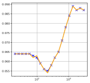
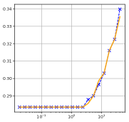
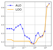
Figure 5: Risk estimates of from ALO versus LOOCV for the three datasets: gisette, South Africa coronary heart disease and colon tumor gene expression. The $x$-axis is the tuning parameter value $\lambda$ on $\log$-scale, the $y$-axis is the risk estimates under 0-1 loss.

There are a few factors which may affect the performance of ALO. First, as implied by the theoretical guarantee on smooth models, the closeness between ALO and LOOCV is a high-dimensional phenomenon, which takes place for relatively large $n$ and $p$. This requirement of high-dimensionality is less stringent for $n>p$, when strong convexity of the loss function is to some extent guaranteed, but becomes more significant for $n<p$. On the other hand, from our simulation in Section 7 and the real-data examples in this section, we can see that when $\frac{n}{p}$ is not much smaller than 1 (compared to the $\frac{n}{p}$-ratio in the colon tissue dataset), a few hundreds of observation and features are enough to guarantee the accuracy of ALO risk estimates. Finally, the deviation of ALO estimates tends to happen when the tuning $\lambda$ becomes smaller than a certain value, typically in the case of $n<p$. As we have mentioned in the main text, for most nonsmooth regularizers, small tuning values induce dense solutions. In most high dimensional datasets, these dense solutions are not favorable in $n<p$ case. From our experiments, this deviation mostly happens after correctly capturing the optimal tuning values.

References

• [1] Davidย M Allen. The relationship between variable selection and data agumentation and a method for prediction. Technometrics, 16(1):125โ€“127, 1974.
• [2] Uri Alon, Naama Barkai, Danielย A Notterman, Kurt Gish, Suzanne Ybarra, Daniel Mack, and Arnoldย J Levine. Broad patterns of gene expression revealed by clustering analysis of tumor and normal colon tissues probed by oligonucleotide arrays. Proceedings of the National Academy of Sciences, 96(12):6745โ€“6750, 1999.
• [3] Dennis Amelunxen, Martin Lotz, Michaelย B McCoy, and Joelย A Tropp. Living on the edge: Phase transitions in convex programs with random data. Information and Inference: A Journal of the IMA, 3(3):224โ€“294, 2014.
• [4] Mohsen Bayati, Muratย A Erdogdu, and Andrea Montanari. Estimating lasso risk and noise level. In Advances in Neural Information Processing Systems, pages 944โ€“952, 2013.
• [5] Stephenย R. Becker, Emmanuelย J. Candรจs, and Michaelย C. Grant. Templates for convex cone problems with applications to sparse signal recovery. Math. Program. Comput., 3(3):165โ€“218, 2011.
• [6] Ahmad Beirami, Meisam Razaviyayn, Shahin Shahrampour, and Vahid Tarokh. On optimal generalizability in parametric learning. In Advances in Neural Information Processing Systems, pages 3458โ€“3468, 2017.
• [7] Stephen Boyd and Lieven Vandenberghe. Convex optimization. Cambridge University Press, Cambridge, 2004.
• [8] Emmanuelย J Candes, Carlosย A Sing-Long, and Joshuaย D Trzasko. Unbiased risk estimates for singular value thresholding and spectral estimators. IEEE transactions on signal processing, 61(19):4643โ€“4657, 2013.
• [9] Gavinย C Cawley and Nicolaย LC Talbot. Efficient approximate leave-one-out cross-validation for kernel logistic regression. Machine Learning, 71(2-3):243โ€“264, 2008.
• [10] Chih-Chung Chang and Chih-Jen Lin. Libsvm: a library for support vector machines. ACM transactions on intelligent systems and technology (TIST), 2(3):27, 2011.
• [11] Patrickย L. Combettes and Jean-Christophe Pesquet. Proximal Splitting Methods in Signal Processing, pages 185โ€“212. Springer New York, New York, NY, 2011.
• [12] Corinna Cortes and Vladimir Vapnik. Support-vector networks. Machine learning, 20(3):273โ€“297, 1995.
• [13] Davidย L Donoho, Arian Maleki, and Andrea Montanari. Message-passing algorithms for compressed sensing. Proceedings of the National Academy of Sciences, 106(45):18914โ€“18919, 2009.
• [14] Davidย L Donoho and Jared Tanner. Neighborliness of randomly projected simplices in high dimensions. Proceedings of the National Academy of Sciences of the United States of America, 102(27):9452โ€“9457, 2005.
• [15] Charles Dossal, Maher Kachour, MJย Fadili, Gabriel Peyrรฉ, and Christophe Chesneau. The degrees of freedom of the lasso for general design matrix. Statistica Sinica, pages 809โ€“828, 2013.
• [16] Bradley Efron. The estimation of prediction error: covariance penalties and cross-validation. Journal of the American Statistical Association, 99(467):619โ€“632, 2004.
• [17] Michael Grant and Stephen Boyd. CVX: Matlab software for disciplined convex programming, version 2.1. http://cvxr.com/cvx, March 2014.
• [18] Isabelle Guyon, Steve Gunn, Asa Ben-Hur, and Gideon Dror. Result analysis of the nips 2003 feature selection challenge. In Advances in neural information processing systems, pages 545โ€“552, 2005.
• [19] Williamย W Hager. Updating the inverse of a matrix. SIAM review, 31(2):221โ€“239, 1989.
• [20] Trevor Hastie, Robert Tishirani, and Jerome Friedman. Elements of Statistical Learning, chapter Model Assessment and Selection. Springer-Verlag New York, 2 edition, 2009.
• [21] Trevor Hastie, Robert Tishirani, and Jerome Friedman. Elements of Statistical Learning, chapter Linear Methods for Classification. Springer-Verlag New York, 2 edition, 2009.
• [22] Peterย J Huber. Robust regression: asymptotics, conjectures and monte carlo. The Annals of Statistics, pages 799โ€“821, 1973.
• [23] Seung-Jean Kim, Kwangmoo Koh, Stephen Boyd, and Dimitry Gorinevsky. $l_{1}$ trend filtering. SIAM Rev., 51(2):339โ€“360, 2009.
• [24] Guanghui Lan, Zhaosong Lu, and Renato D.ย C. Monteiro. Primal-dual first-order methods with $\mathcal{O}(1/\epsilon)$ iteration-complexity for cone programming. Mathematical Programming, 126(1):1โ€“29, Jan 2011.
• [25] Saskia Leย Cessie and Johannesย C Vanย Houwelingen. Ridge estimators in logistic regression. Applied statistics, pages 191โ€“201, 1992.
• [26] Adrianย S Lewis. The convex analysis of unitarily invariant matrix functions. Journal of Convex Analysis, 2(1):173โ€“183, 1995.
• [27] Rosaย J Meijer and Jelleย J Goeman. Efficient approximate k-fold and leave-one-out cross-validation for ridge regression. Biometrical Journal, 55(2):141โ€“155, 2013.
• [28] Lย Mirsky. Symmetric gauge functions and unitarily invariant norms. Quarterly Journal of Mathematics, 11:50โ€“59, 1960.
• [29] Ali Mousavi, Arian Maleki, Richardย G Baraniuk, etย al. Consistent parameter estimation for lasso and approximate message passing. The Annals of Statistics, 45(6):2427โ€“2454, 2017.
• [30] Tomoyuki Obuchi and Yoshiyuki Kabashima. Cross validation in lasso and its acceleration. Journal of Statistical Mechanics: Theory and Experiment, 2016(5):053304, 2016.
• [31] Manfred Opper and Ole Winther. Gaussian processes and svm: Mean field results and leave-one-out. 2000.
• [32] Finbarr Oโ€™sullivan, Brianย S Yandell, and Williamย J Raynorย Jr. Automatic smoothing of regression functions in generalized linear models. Journal of the American Statistical Association, 81(393):96โ€“103, 1986.
• [33] F.ย Pedregosa, G.ย Varoquaux, A.ย Gramfort, V.ย Michel, B.ย Thirion, O.ย Grisel, M.ย Blondel, P.ย Prettenhofer, R.ย Weiss, V.ย Dubourg, J.ย Vanderplas, A.ย Passos, D.ย Cournapeau, M.ย Brucher, M.ย Perrot, and E.ย Duchesnay. Scikit-learn: Machine learning in Python. Journal of Machine Learning Research, 12:2825โ€“2830, 2011.
• [34] Junyang Qian, Tย Hastie, Jย Friedman, Rย Tibshirani, and Nย Simon. Glmnet for matlab 2013. URL http://www. stanford. edu/~ hastie/glmnet_matlab, 2013.
• [35] Kamiar Rad and Arian Maleki. A scalable estimate of the extra-sample prediction error via approximate leave-one-out. arXiv preprint arXiv:1801.10243, 2018.
• [36] R.ย Tyrrell Rockafellar. Convex analysis. Princeton Mathematical Series, No. 28. Princeton University Press, Princeton, N.J., 1970.
• [37] JEย Rossouw, JPย Duย Plessis, AJย Benadรฉ, PCย Jordaan, JPย Kotze, PLย Jooste, and JJย Ferreira. Coronary risk factor screening in three rural communities. the coris baseline study. South African medical journal= Suid-Afrikaanse tydskrif vir geneeskunde, 64(12):430โ€“436, 1983.
• [38] Mervyn Stone. Cross-validatory choice and assessment of statistical predictions. Journal of the royal statistical society. Series B (Methodological), pages 111โ€“147, 1974.
• [39] Robert Tibshirani. Regression shrinkage and selection via the lasso. Journal of the Royal Statistical Society. Series B (Methodological), pages 267โ€“288, 1996.
• [40] Robert Tibshirani, Michael Saunders, Saharon Rosset, Jiย Zhu, and Keith Knight. Sparsity and smoothness via the fused lasso. J. R. Stat. Soc. Ser. B Stat. Methodol., 67(1):91โ€“108, 2005.
• [41] Ryanย J. Tibshirani and Jonathan Taylor. The solution path of the generalized lasso. Ann. Statist., 39(3):1335โ€“1371, 2011.
• [42] Ryanย J Tibshirani, Jonathan Taylor, etย al. Degrees of freedom in lasso problems. The Annals of Statistics, 40(2):1198โ€“1232, 2012.
• [43] Samuel Vaiter, Charles Deledalle, Jalal Fadili, Gabriel Peyrรฉ, and Charles Dossal. The degrees of freedom of partly smooth regularizers. Annals of the Institute of Statistical Mathematics, 69(4):791โ€“832, 2017.
• [44] Lย Weyl. Das asymptotische verteilungsgestez der eigenwert linearer partieller differentialgleichungen (mit einer anwendung auf der theorie der hohlraumstrahlung). Mathematische Annalen, 71:441โ€“479, 1912.
• [45] Maxย A Woodbury. Inverting modified matrices. Memorandum report, 42(106):336, 1950.
• [46] Hui Zou, Trevor Hastie, Robert Tibshirani, etย al. On the โ€œdegrees of freedomโ€ of the lasso. The Annals of Statistics, 35(5):2173โ€“2192, 2007.