An Image Encryption Algorithm Based on Chaotic Maps and Discrete Linear Chirp Transform

Abstract

In this paper, a novel image encryption algorithm, which involves a chaotic block image scrambling followed by a two–dimensional (2D) discrete linear chirp transform, is proposed. The definition of the 2D discrete linear chirp transform is introduced and then it is used to construct the basis of the novel encryption algorithm. Finally, security analysis are performed to show the quality of the encryption process using different metrics.

I Introduction

With the rapid development of digital technologies and Internet, information security including image encryption has become more and more important. The traditional encryption algorithms such as data encryption standard (DES), advanced encryption standard (AES), and public key encryption algorithm (RSA) are not suitable for image encryption because the digital image has intrinsic properties such as bulk data capacities, high redundancy, and strong correlation between the adjacent pixels [1, 2]. Therefore, many encryption methods relying on different approaches have been introduced in literature to fulfil the security requirements of digital images. Among these approaches, encryption algorithms based on spatial domain [3, 4], frequency domain [6, 7], and fractional domain [8] have been proposed for encryption algorithm design.

In spatial domain methods, the encryption algorithm works on the pixels of plain image directly, while the frequency domain schemes act on the coefficients of the transformed image which can be attained using transformation tools such as fast Fourier transform (FFT), discrete cosine transform (DCT), and discrete wavelet transform (DWT). On the other hand, the fractional domain approaches can give greater complexity to the system by giving an extra parameter of the transform order, which enlarges the key space resulting in a better and secure data protection as compared to the spatial and frequency domain methods. The most widely investigated fractional transform is the fractional Fourier transform, which has a well established continuous–time version and also several definitions in the discrete–time framework.

In recent years, many different fractional Fourier transform encryption schemes have been proposed. In [9], Zhu et al. proposed an optical image encryption method based on multi–fractional Fourier transforms (MFRFT). Pei and Hsue presented an image encryption method based on multiple–parameter discrete fractional Fourier transform (MPDFRFT) [10]. In [11], Liu et al. introduced a random fractional Fourier transform (RFRFT) by using random phase modulations. The results in [12] have shown that these image encryption schemes had deficiencies. Therefore, many encryption algorithms based on the FrFT were suggested to enhance security [13, 14, 15, 16, 18, 19].

In this paper, the definition of the 2D discrete linear chirp transform (2D-DLCT) is proposed and an image encryption scheme based on such transform is introduced. The 2D-DLCT is an extension to the 1D discrete linear chirp transform given in [20], which has an excellent property in a sense that the chirp rate parameter ideally can have infinity support such that $-\infty<\beta<+\infty$ compared to the support of the fractional order of the fractional Fourier transform $0\leq\alpha\leq\pi/2$. In the proposed encryption scheme, the plain image is scrambled using chaotic logistic map which has three secret keys. The scrambled image is 2D-DLCT transformed using $\beta_{x}$ and $\beta_{y}$ chirp rates. These chirp rates serves as a secret keys as well. Then the transformed image is scrambled using different logistic map with another set of secret keys. Numerical results show the proposed scheme can be infeasible to the brute–force attack, more secure, and can resist noise and occlusion attacks.

The remainder of this paper is organized as follows. In section II, the definition of the 2D discrete Linear chirp transform is introduced. Section III presents the details of the proposed image encryption scheme. Section IV gives the numerical simulations and results to demonstrate the performance and verify the validity of the proposed scheme. The conclusion is drawn and stated in section V.

II 2D Discrete Linear Chirp Transform (2D-DLCT)

Let $x(n,m)$ be a two–dimensional discrete signal, where $n=0,1,\cdots,N-1$ and $m=0,1,\cdots,M-1$. The two–dimensional discrete linear chirp transform of the signal $x(n,m)$ with chirp rates $\beta_{x}$ for the x–axis and $\beta_{y}$ for the y–axis is defined as

$$X(k,\ell)=\sum_{n=0}^{N-1}\sum_{m=0}^{M-1}x(n,m)~{}\mathcal{K}_{\beta_{x},\beta_{y}}(n,m,k,\ell)$$ (1)

with the kernel

$$\mathcal{K}_{\beta_{x},\beta_{y}}(n,m,k,\ell)=\mathcal{K}_{\beta_{x}}(n,k)~{}\mathcal{K}_{\beta_{y}}(m,\ell)$$ (2)

where,

$$\mathcal{K}_{\beta_{x}}(n,k)=\exp\left(-\frac{2\pi}{N}(k~{}n+\beta_{x}~{}n^{2})\right)$$ (3)

and

$$\mathcal{K}_{\beta_{y}}(m,\ell)=\exp\left(-\frac{2\pi}{M}(\ell~{}m+\beta_{y}~{}m^{2})\right)$$ (4)

The chirp rates $\beta_{x}$ and $\beta_{y}$ are real numbers which can take any value from their support $-\infty<\beta_{x},~{}\beta_{y}<\infty$. The 2D-DLCT can be expressed as a tensor product of two one–dimensional transforms. The inverse 2D-DLCT is obtained using the following mathematical expression

$$x(n,m)=\sum_{k=0}^{N-1}\sum_{\ell=0}^{M-1}X(k,\ell)~{}\mathcal{K}_{\beta_{x},\beta_{y}}^{*}(n,m,k,\ell)$$ (5)

where $0\leq k\leq N-1$, $0\leq\ell\leq M-1$, and ($*$) denotes the conjugate.

III The Proposed Encryption and Decryption Algorithm

The proposed image encryption scheme is illustrated in Fig. 1(a). It employs the 2D-DLCT developed in Section II and additional strategies such as pixel rearrangement in the spatial and chirp rate domains using the well known chaotic logistic maps. The logistic map is a one–dimensional nonlinear chaos function and is defined as [3]

$$x_{i+1}=\mu x_{i}(1-x_{i})$$ (6)

where $\mu$ is the system parameter sometimes known as bifurcation parameter and $x_{i}\epsilon(0,1)$ is the sequence value. When $3.5699456\leq\mu\leq 4$, slight variations in the initial value yield dramatically different results over time. That is to say, logistic map will operate in chaotic state. With $x_{0}$ being the initial value, a non–periodic sequence $\{x_{i};i=0,1,2,3,\cdots\}$ sensitive to the initial value is generated.

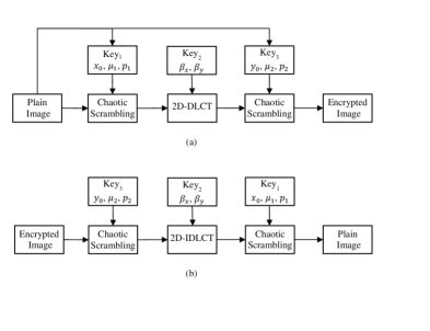
Figure 1: Schematic diagram of the proposed algorithm: (a) Encryption process, (b) Decryption process.

Without loss of generality, the size of the plain image I is an $N\times M$ and the encryption procedure is described as follows:

• Setting the initial values of the chaotic system by means of the plain image $I$ to increase the relationship between the encryption scheme and the plain image.

• Given the initial parameter $x_{0}$ and $\mu_{1}$, generate a random sequence $x=\{x_{1},x_{2},\cdots,x_{L}\}$, where $L>N\times M$, and discard the first $p_{1}$ values. A new sequence $v=\{v_{1+p_{1}},v_{2+p_{2}},\cdots,v_{NM+p_{1}}\}$ is obtained. The parameters $x_{0}$, $\mu_{1}$, and $p_{1}$ serve as a first private key (key₁).

• Sort the sequence $v$ in ascending order or descending order to form a new sequence. Thus, the positions of the elements are varied and the positions are recorded as $IX$.

• Reshape the plain image $I_{N\times M}$ into a vector $S_{NM\times 1}$, and then use the scrambling index $IX$ to reorder the items of the vector $S$. The scrambled image in the spatial domain can be obtained by reconverting $S$ into an $N\times M$ matrix $E$.

• Choose two real numbers for $\beta_{x}$ and $\beta_{y}$, which serve as a second private key (key₂), and employ them to transform the image $E$ using 2D-DLCT.

• Scramble the attained matrix as explained in the previous steps using different set of initial values, that is $y_{0}$, $\mu_{2}$, and $p_{2}$ which represent the third private key (key₃).

• Finally, the encrypted image is obtained by converting the scrambled vector into an $N\times M$ matrix $Y$.

The decryption algorithm is the inverse operation of the encryption as shown in Fig. 1(b).

IV Simulation Results and Security Analysis

In the simulations, a standard Lena test image of size $256\times 256$ [21] that has allocation of $8$ bits/pixel of gray–scale is used. The parameters of the chaotic logistic map and the chirp rates of the 2D-DLCT which employed in the simulation experiments are listed in Table I.

TABLE I: Simulation parameters.

Parameter	Value
$x_{0}$	$0.31$
$\mu_{1}$	$3.8$
$p_{1}$	$\mod(\sum_{i,j}I_{ij},9999)$
$y_{0}$	$0.25$
$\mu_{2}$	$3.7$
$p_{2}$	$\mod(\sum_{i,j}I_{ij},9990)$
$\beta_{x}$	$1.5$
$\beta_{y}$	$-3.5$

Figures 2(a), (b), and (c) show the plain image, encrypted image, and decrypted image, respectively. In the following subsections, the security analysis of the proposed encryption scheme is performed to check its resistance to various attacks.

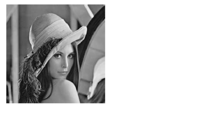
(a)

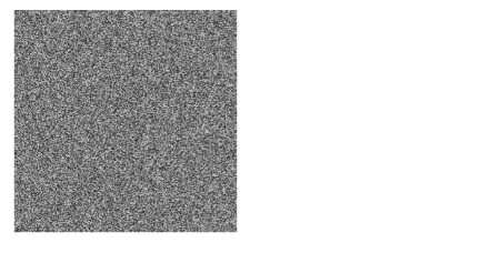
(b)

(c)

Figure 2: Encryption and decryption results. (a) Plain image. (b) Encrypted image. (c) Decrypted image.

IV-A Key Space Analysis

Key space size is the total number of different keys that can be used in an encryption algorithm. In a cryptographic system, the key space should be sufficiently large to make brute–force attack infeasible. The proposed encryption algorithm have the following secret keys: key${}_{1}=\{x_{0},\mu_{1},p_{1}\}$, key${}_{2}=\{\beta_{x},\beta_{y}\}$ , and key${}_{3}=\{y_{0},\mu_{2},p_{2}\}$ and their corresponding spaces are $s_{1}$, $s_{2}$, $s_{3}$, $s_{4}$, $s_{5}$, $s_{6}$, $s_{7}$, and $s_{8}$ , respectively. These keys are independent from each other. Thus the total key space of the encryption scheme can be computed as

$$s>\prod_{i}s_{i}$$ (7)

If we assume the computation precision of the computer is $10^{-14}$, then the key space is about $10^{74}\approx 2^{245}$. Such a large key space can ensure a high security against brute–force attacks [22].

IV-B Key Sensitivity Analysis

A good encryption scheme should be sensitive to each secret key. In other words, a small change on the key must be able to cause a great change on the encrypted image. In order to evaluate the key sensitivity of the proposed algorithm, the mean square error (MSE) between the plain image and decrypted image is calculated as follows

$$\mbox{MSE}=\frac{1}{N\times M}\sum_{i=1}^{N}\sum_{j=1}^{M}|I(i,j)-D(i,j)|^{2}$$ (8)

where $I(i,j)$ is the plain image and $D(i,j)$ denotes the corresponding decrypted image. To determine the sensitivity of the key parameters, the decryption procedure is processed by varying one parameter while the others held constant.

Figures 3(a), (b), (c), and (d) show the MSE versus deviation of the key encryption parameters $\beta_{x}$, $x_{0}$, $\mu_{1}$, and $p_{1}$, respectively. Since the MSE increases sharply when the the key parameters depart from its correct value and it is equal to zero when the image is decrypted with correct decryption parameters, a small change to the keys can lead to different decrypted image having no connection with the original image.

It should be noted that we omit the sensitivity analysis of the remaining key parameters $y_{0}$, $\mu_{2}$, and $p_{2}$ because they give similar results to those shown with the key parameters $x_{0}$, $\mu_{1}$, and $p_{1}$.

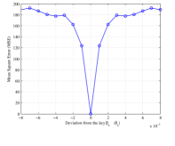
(a)

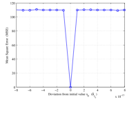
(b)

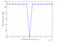
(c)

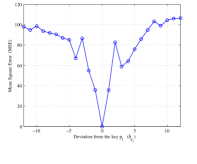
(d)

Figure 3: MSE for deviation of the correct keys. (a) Chirp rate $\beta_{x}$. (b) Initial value $x_{0}$. (c) Logistic map function parameter $\mu_{1}$. (d) Truncated position $p_{1}$.

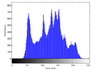
(a)

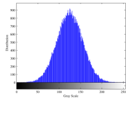
(b)

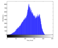
(c)

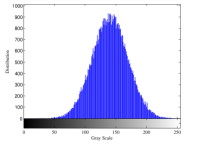
(d)

Figure 4: Examples of histograms. (a) Lena image. (b) Encrypted image of Lena. (c) Baboon image. (d) Encrypted image of Baboon.

IV-C Histogram Analysis

To resist statistical attacks, the encrypted images should have histograms that are consistent in distribution and are different from the histograms of their plain images. Figure 4(a) and (c) show the histograms of Lena and Baboon plain images respectively, while Fig. 4(b) and (d) present the histograms of their encrypted images. It is clear that the histograms of the plain images are different from each other and their corresponding encrypted images have similar statistical properties. Moreover, the values of the encrypted image are subject to normal distribution. Hence, the encrypted image histogram data does not provide any useful information for the attackers to perform any statistical analysis attack on the encrypted image.

IV-D Correlation Analysis

To evaluate the correlation of adjacent pixels, $6000$ pairs of adjacent pixels are randomly selected from both the plain and encrypted images. A good encrypted image must have low correlation for the three directions-– horizontal, vertical and diagonal. The distribution of two adjacent pixels to the plain and encrypted images for the three directions is shown in Fig. 5(a)–(f). Thus, correlation plots of plain images exhibit clear patterns while those of their encrypted counterparts show no clear pattern, the points being rather randomly distributed.

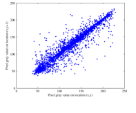
(a)

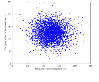
(b)

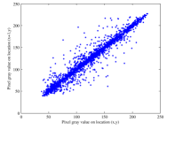
(c)

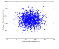
(d)

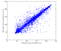
(e)

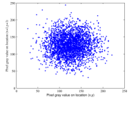
(f)

Figure 5: Correlation coefficients of plain and encrypted Lena images, from top to bottom: in horizontal, vertical, and diagonal direction, respectively.

In order to test the correlations of adjacent pixels for the plain and encrypted images, the correlation coefficients $r_{xy}$ of each pair are calculated using the following equations

$$r_{xy}=\frac{\sum_{i=1}^{L}(x_{i}-\bar{x})(y_{i}-\bar{y})}{\sqrt{\left[\sum_{i=1}^{L}(x_{i}-\bar{x})^{2}\right]\left[\sum_{i=1}^{L}(y_{i}-\bar{y})^{2}\right]}}$$ (9)

where $\bar{x}=1/L\sum_{i=1}^{L}x_{i}$, $\bar{y}=1/L\sum_{i=1}^{L}y_{i}$, $x_{i}$ is the value of the i-th selected pixel, $y_{i}$ is the value of the correspondent adjacent pixel, and $L$ is the total number of pixels selected from the image. The correlation coefficients of the plain image and encrypted image are summarized in Table II.

TABLE II: Correlation coefficients of two adjacent pixels in the plain and encrypted images.

Image and scheme	Horizontal	Vertical	Diagonal
Plain Lena	$0.9481$	$0.9737$	$0.9244$
Encrypted Lena	$-0.0014$	$0.0025$	$0.0051$
Plain Baboon	$0.8701$	$0.8411$	$0.7889$
Encrypted Baboon	$0.0077$	$-0.002$	$-0.0039$
Plain Cameraman	$0.9556$	$0.9738$	$0.934$
Encrypted Cameraman	$-5.84\times 10^{-4}$	$-0.0077$	$0.0015$
Plain Pirate	$0.9434$	$0.9564$	$0.9134$
Encrypted Pirate	$-0.002$	$5.25\times 10^{-4}$	$-0.0048$

The importance of this work is also emphasised through the values of the correlation coefficient in Table III. It is clear that the correlation coefficient of the proposed algorithm is smaller than that of other methods proposed in Refs. [17, 16, 23, 24, 25, 26].

TABLE III: Correlation coefficient of the proposed algorithm compared to others using plain Lena image.

Algorithm	Horizontal	Vertical	Diagonal
Proposed algorithm	$-0.0014$	$0.0025$	$0.0051$
Ref. [17]	$0.002$	$0.0062$	$0.0066$
Ref. [16]	$-0.0069$	$-0.0188$	$-0.0482$
Ref. [23]	$-0.0274$	$0.0046$	$-0.0038$
Ref. [24]	$0.319$	$0.3314$	$0.0149$
Ref. [25]	$-0.0016$	$-0.0033$	$0.0130$
Ref. [26]	$-0.0226$	$0.0041$	$0.0368$

IV-E Occlusion Attack Analysis

To test the robustness of the proposed encryption algorithm against loss of data, we occlude $25\%$, $50\%$, and $75\%$ of the encrypted image pixels. The decryption process is performed on the occluded encrypted image of “Lena" with all correct private keys. The encrypted images with $25\%$, $50\%$, and $75\%$ data losses are shown in Fig. 6(a), (c), and (e) while the corresponding recovered images are illustrated in Fig. 6(b), (d), and (f), respectively. The decrypted images is recognisable even when the encrypted image is occluded up to $75\%$, though the quality of recovered images drops with the increase in occluded area. We employ the peak signal–to–noise ratio (PSNR) to compute the quality of the recovered image after attack. For a grayscale image, the PSNR may be computed using the following mathematical expression,

$$\mbox{PSNR}=10~{}\log_{10}\left(\frac{255^{2}}{\mbox{MSE}}\right)$$ (10)

where MSE is defined in Eq. (8). The results of resisting occlusion attack of the proposed algorithm compared to others are presented in Table IV.

(a)

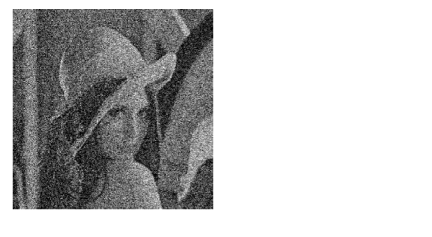
(b)

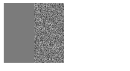
(c)

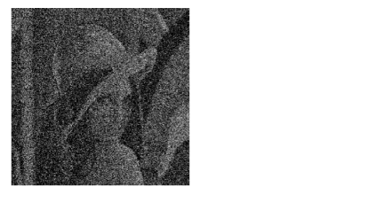
(d)

(e)

(f)

Figure 6: Occlusion attack analysis. (a) Encrypted image with $25\%$ occlusion. (b) Decrypted image from (a). (c) Encrypted image with $50\%$ occlusion. (d) Decrypted image from (c). (e) Encrypted image with $75\%$ occlusion. (f) Decrypted image from (e).

TABLE IV: Comparison between the PSNR of the reconstructed images with different block size data loss.

	PSNR (dB)
Occlusion (%)
	Proposed	Ref. [14]	Ref. [27]
$25$	$25.70$	$13.88$	$15.42$
$50$	$24.82$	$11.27$	$11.26$
$75$	$24.33$	$9.60$	$7.05$

IV-F Noise Attack Analysis

The robustness of the proposed encryption algorithm is also tested against noise attack. The encrypted Lena image is added to a zero mean Gaussian noise with different intensities. Fig. 7(a)–(d) show decrypted images with noise intensity $0.01$, $0.05$, $0.1$, and $0.2$, respectively. The PSNR values of the proposed scheme and the schemes in [28] and [29] are compared in Table V, which shows that the proposed scheme has better performance at high levels of Gaussian noise. Thus, the results demonstrate that the proposed scheme can resist the noise attack.

(a)

(b)

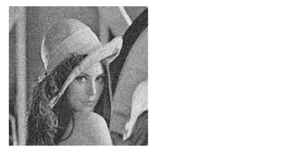
(c)

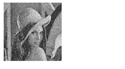
(d)

Figure 7: Decrypted images with different levels of Gaussian noise. (a) $\sigma=0.01$. (b) $\sigma=0.05$. (c) $\sigma=0.1$. (d) $\sigma=0.2$.

TABLE V: The PSNR of decrypted images under different noise levels.

	PSNR (dB)
Intensity (%)
	Proposed	Ref. [28]	Ref. [29]
$0.01$	$43.97$	$30.59$	$38.93$
$0.05$	$32.36$	$28.55$	$33.64$
$0.1$	$29.42$	$25.33$	$29.57$
$0.2$	$27.95$	$20.58$	$26.95$
$0.25$	$27.52$	$18.91$	$23.88$

V Conclusion

In summary, an image encryption scheme has been proposed based on logistic maps and 2D discrete Linear chirp transform. It is demonstrated that the proposed scheme ensures, feasibility, security, and robustness by performing simulations for grayscale images. The results show that the scheme is infeasible to the brute–force attack and offers a great degree of security as seen from its statistical analysis and sensitivity to the encryption parameters. Finally, it has been illustrated that the proposed method is robust against noise and occlusion attacks.

References

- [1] N. K. Pareek, V. Patidar, and K. K. Sud, “Image encryption using chaotic logistic map," Image and Vision Computing, Vol. 24, no. 9, pp. 926934, Sep. 2006.
- [2] H. Yang, K-W Wong, X. Liao, W. Zhang, and P. Wei, “A fast image encryption and au- thentication scheme based on chaotic maps," Communications in Nonlinear Science and Numerical Simulation, Vol. 15, no. 11, pp. 35073517, Nov. 2010.
- [3] R. Matthews, “ On the derivation of a chaotic encryption algorithm," Cryptologia, Vol. 13, no. 1, pp. 2942, Jan. 1989.
- [4] Z-I Zhu, W. Zhang, K-W Wong, and H. Yu, “A chaos–based symmetric image encryption scheme using a bit–level permutation," Information Sciences, Vol. 181, no. 6, pp. 11711186, Mar. 2011.
- [5] Z. Liu, L. Xu, T. Liu, H. Chen, P. Li, C. Lin, and S. Liu, “Color image encryption by using Arnold transform and color–blend operation in discrete cosine transform domains," Optics Communication, Vol. 284, no. 1, pp. 123128, Jan. 2011.
- [6] P. Refregier, “ Optical image encryption based on input plane and Fourier plane random encoding," Optics Letters, Vol. 20, no. 7, pp. 767769, Apr. 1995.
- [7] Y. Luo, M. Du, and J. Liu, “ A symmetrical image encryption scheme in wavelet and time domain," Communications in Nonlinear Science Numerical Simulation, Vol. 20, no. 2, pp. 447460, May 2015.
- [8] G. Unnikrishnan, J. Joseph, and K. Singh, “Optical encryption by double–random phase encoding in the fractional Fourier domain," Optics Letters, Vol. 25, no. 12, pp. 887889, Jun. 2000.
- [9] B.H. Zhu, S.T. Liu, and Q.W. Ran, “Optical image encryption based on multifractional Fourier transforms," Optics Letters, Vol. 25, no. 16, pp. 11591161, Aug. 2000.
- [10] S.C. Pei and W.L. Hsue, “The multiple–parameter discrete fractional Fourier transform," IEEE Signal Processing Letters, Vol. 13, no. 6, pp. 329332, Jun. 2006.
- [11] Z. Liu and S. Liu, “Random fractional Fourier transform," Optics Letters, Vol. 32, no. 15, pp. 20882090, Aug. 2007.
- [12] Q. Ran, H. Zhang, J. Zhang, L. Tan, and J. Ma, “Deficiencies of the cryptography based on multiple–parameter fractional Fourier transform," Optics Letters, Vol. 34, no. 11, pp. 17291731, Jun. 2009.
- [13] N. Zhou, Y. Wang, L. Gong, H. He, and J. Wu, “Novel single–channel color image encryption algorithm based on chaos and fractional Fourier transform," Optics Communications, Vol. 284, no. 12, pp. 27892796, Jun. 2011.
- [14] J. Lang, “Image encryption based on the reality–preserving multiple-parameter fractional Fourier transform and chaos permutation," Optics and Lasers in Engineering, Vol. 50, no. 7, pp. 929937, Jul. 2012.
- [15] A. Elshamy, A. Rashed, A. Mohamed, O. Faragallah, Y. Mu, S. Alshebeili, and F. Abd El-samie, “Optical image encryption based on chaotic baker map and double random phase encoding," Journal of Lightwave Technology, Vol. 31, no. 15, pp. 25332539, Aug. 2013.
- [16] L. Sui, H. Lu, Z. Wang, and Q. Sun, “Double–image encryption using discrete fractional random transform and logistic maps," Optics and Lasers in Engineering, Vol. 56, pp. 112, May 2014.
- [17] J. Lima and L. Novaes, “Image encryption based on the fractional Fourier transform over finite fields," Signal Processing, Vol. 94, no. , pp. 521530, 2014.
- [18] Y. Li, F. Zhang, Y. Li, and R. Tao, “Asymmetric multiple–image encryption based on the cascaded fractional Fourier transform," Optics and Lasers in Engineering, Vol. 72, pp. 1825, Apr. 2015.
- [19] T. Zhao, Q. Ran, L. Yuan, Y. Chi, and J. Ma, “Security of image encryption scheme based on multi–parameter fractional Fourier transform," Optics Communications, Vol. 376, pp. 4751, May 2016.
- [20] O. A. Alkishriwo, A. Akan, and L. F. Chaparro, “Intrinsic mode chirp decomposition of non–stationry signals", IET Signal Processing, vol. 8, no. 3, pp. 267276, May. May 2014.
- [21] Image Database /http://www.imageprocessingplace.com/index.htm
- [22] G. Alvarez and S. Li, “Some basic cryptographic requirements for chaos-based cryptosystems," International Journal Bifurcation and Chaos, Vol. 16, no. 8, pp. 21292151, 2006.
- [23] B. Nini and C. Lemmouchi, “Security analysis of a three–dimensional rotation–based image encryption," IET Image Processing, Vol. 9, no. 8, pp. 680689, Aug. 2015.
- [24] M. H. Annaby, M. A. Rushdi, and E. A. Nehary, “Image encryption via discrete fractional Fourier–type transforms generated by random matrices," Signal Processing: Image Communication, Vol. 49, pp. 2546, Nov. 2016.
- [25] X. Chai, Z. Gan, K. Yang, Y. Chen, and X. Liu, “An image encryption algorithm based on the memristive hyperchaotic system, cellular automata, and DNA sequence operations," Signal Processing: Image Communication, Vol. 52, pp. 619, Mar. 2017.
- [26] L. Xu, X. Gou, Z. Li, and J. Li,“A novel chaotic image encryption algorithm using block scrambling and dynamix index based diffusion," Optics and Lasers in Engineering, Vol. 79, pp. 4152, Apr. 2017.
- [27] N. Rawat, B. Kim, and Rajesh Kumar, “Fast digital image encryption based on compressive sensing using structurally random matrices and Arnold transform technique," Optik–International Journal of Light and Electron Optics, Vol. 127, no. 4, pp. 22822286, Feb. 2016.
- [28] N. Zhou, S. Pan, S. Cheng, Z. Zhou, “Image compression–-encryption scheme based on hyper–chaotic system and 2D compressive sensing," Optics and Laser Technology, Vol. 82, pp. 121133, Aug. 2016.
- [29] D. Xiao, L. Wang, T. Xiang, and Y. Wang, “Multi–focus image fusion and robust encryption algorithm based on compressive sensing," Optics and Laser Technology, Vol. 91, pp. 212225, Jun. 2017.