Quantum sensing enhanced by adaptive periodic quantum control

Abstract

Using a single quantum probe to sense other quantum objects offers distinct advantages but suffers from some limitations that may degrade the sensing precision severely, especially when the probe-target coupling is weak. Here we propose a strategy to improve the sensing precision by using the quantum probe to engineer the evolution of the target. We consider an exactly solvable model, in which a qubit is used as the probe to sense the frequency of a harmonic oscillator. We show that by applying adaptive periodic quantum control on the qubit, the sensing precision can be enhanced from $1/T$ scaling with the total time cost $T$ to $1/T^{2}$ scaling, thus improving the precision by several orders of magnitudes. Such improvement can be achieved without any direct access to the oscillator and the improvement increases with decreasing probe-target coupling. This provides a useful routine to ultrasensitive quantum sensing of weakly coupled quantum objects.

Using single quantum objects as quantum probes for sensing provides distinct advantages, e.g., high spatial resolution Taylor et al. (2008); Balasubramanian et al. (2008); Maze et al. (2008), integrability, and miniature of devices, in comparison with macroscopic probes. Due to recent experimental progress in controlling single quantum objects, such as single trapped ions, superconducting qubits, and single defect spins in solids Robledo et al. (2011); Togan et al. (2010, 2011); Maze et al. (2011); O’Brien et al. (2001); Morello et al. (2010), atomic scale sensing with single quantum probes is now made possible Degen et al. (2017), and may trigger new applications in broad fields including chemistry, biology and material sciences. However, the widely used quantum resources – large-scale entanglement and interactions among different quantum probes – are no longer available for a single quantum probe. Moreover, a large family of tasks requires sensing quantum objects weakly coupled to the quantum probe, where direct access (e.g., initialization, manipulation, or measurement) to the target quantum object is not available. These limitations may severely degrade the key figure of merit – the sensing precision. It is important to identify and utilize available resources to improve the sensing precision of single quantum probes for weakly coupled quantum objects.

The coherent evolution time $T$ is an important quantum resource. Previous works Zhao et al. (2011, 2012); Taminiau et al. (2012); Kolkowitz et al. (2012a); Cai et al. (2013); London et al. (2013); Laraoui et al. (2013); Shi et al. (2014); Lang et al. (2015); Boss et al. (2016); Zaiser et al. (2016); Ma and Liu (2016a, b); Shu et al. (2017); Liu et al. (2017) on sensing quantum objects mostly use non-adaptive schemes and their precision is upper bounded by a $1/T$ time scaling. By contrast, for sensing classical signals, recent theoretical works show that using adaptive techniques allows universal $1/T$ scaling Yuan and Fung (2015); Yuan (2016) (and $1/T^{2}$ scaling for special tasks Pang and Jordan (2017)), consistent with available experimental reports Nusran et al. (2012); Waldherr et al. (2012); Bonato et al. (2016). However, they are not applicable to sensing weakly coupled quantum objects due to the lack of direct access to the target. Remarkably, a recent breakthrough improves the time scaling to $1/T^{3/2}$ by using the continuous sampling technqiue Schmitt et al. (2017); Boss et al. (2017).

In this work, we propose a strategy for improving the precision for sensing weakly coupled quantum objects. The key is to combine periodic quantum control on the quantum probe Zhao et al. (2011, 2012); Taminiau et al. (2012); Kolkowitz et al. (2012a); Cai et al. (2013); London et al. (2013); Laraoui et al. (2013); Shi et al. (2014); Lang et al. (2015); Boss et al. (2016); Zaiser et al. (2016); Ma and Liu (2016a, b) with adaptive techniques to steer the evolution of the target for maximal information flow from the target to the probe. We consider a single qubit as a quantum probe to estimate the frequency $\omega$ of a harmonic oscillator – a paradigmatic hybrid system that has attracted a lot of interest recently Aspelmeyer et al. (2014). We show that applying adaptive periodic control on the qubit improves the time scaling of the precision from $1/T$ to $1/T^{2}$, thus enhancing the precision by several orders of magnitudes. Interestingly, this improvement can be achieved without any direct access to the oscillator, and the improvement increases with decreasing coupling strength between the qubit and the oscillator. This study highlights adaptive periodic quantum control as a useful route for ultra-sensitive quantum sensing of weakly coupled quantum objects.

I Results

I.1 Sensing other quantum objects: limitations and opportunities

A typical protocol to estimate an unknown parameter $\theta$ with a quantum system consists of three steps: (1) The system starts from certain initial state $\hat{\rho}$ and undergoes certain $\theta$-dependent evolution into the final state $\hat{\rho}_{\theta}$. The information in $\hat{\rho}_{\theta}$ is quantified by the quantum Fisher information $\mathcal{F}$ Braunstein and Caves (1994). (2) A measurement on $\hat{\rho}_{\theta}$ gives an outcome randomly sampled from all possible outcomes $\{x_{m}\}$ according to certain measurement distribution $P(x_{m}|\theta)$ conditioned on $\theta$. The information in each outcome is quantified by the classical Fisher information $F=\sum_{m}P(x_{m}|\theta)[\partial_{\theta}\ln P(x_{m}|\theta)]^{2}$ Kay (1993), which obeys $F\leq\mathcal{F}$. (3) Steps (1) and (2) are repeated $\nu$ times and the $\nu$ outcomes are processed to yield an estimator $\theta_{\mathrm{est}}$ to $\theta$. The precision of $\theta_{\mathrm{est}}$ is quantified by its statistical error $\delta\theta$.

For unbiased estimators Kay (1993), the precision $\delta\theta$ is fundamentally limited by the Cramér-Rao bound Helstrom (1976); Braunstein and Caves (1994)

$$\delta\theta\geq\frac{1}{\sqrt{\nu F}}\geq\frac{1}{\sqrt{\nu\mathcal{F}}}.$$ (1)

For optimal performance, optimal initial state and evolution should be used to maximize $\mathcal{F}$, optimal measurements should be designed to make $F=\mathcal{F}$, and optimal unbiased estimators should be used to saturate the first inequality of Eq. (1).

Sensing classical signals amounts to estimating certain parameter of the quantum probe. The simplest example is to estimate a real parameter $\theta$ in the probe Hamiltonian $\theta\hat{H}$. Starting from an initial state $|\psi\rangle$, the quantum probe evolves for an interval $T$ into a final state $|\psi_{\theta}\rangle\equiv e^{-i\theta T\hat{H}}|\psi\rangle$ with $\mathcal{F}=4H_{\mathrm{rms}}^{2}T^{2}$, where $H_{\mathrm{rms}}\equiv(\langle\psi|\hat{H}^{2}|\psi\rangle-\langle\psi|\hat{H}|\psi\rangle^{2})^{1/2}$ is the fluctuation of $\hat{H}$ in the initial state. If the subsequent measurement and estimator are both optimized to avoid information loss, then after $\nu$ repeated measurements, Eq. (1) gives

$$\delta\theta=\frac{1}{2H_{\mathrm{rms}}\sqrt{\nu}T}.$$ (2)

The precision improves with $\nu$ according to the classical scaling $1/\sqrt{\nu}$, but improves with $T$ according to the enhanced scaling $1/T$ due to the linear phase accumulation $e^{-i\theta T\hat{H}}$ Giovannetti et al. (2006).

Sensing other quantum objects amounts to estimating certain parameter of the target quantum object. In this case, the lack of direct access to the target may degrade the sensing precision significantly: (i) The lack of initialization and direct control over the target may degrade $\mathcal{F}$ in the final state; (ii) The lack of direct measurement over the target may cause information loss during the conversion from $\mathcal{F}$ to $F$; (iii) The unintended evolution of the target due to the backaction of the quantum probe may further degrade $\mathcal{F}$. To illustrate (iii), we consider using a quantum probe with Hamiltonian $\hat{H}_{\mathrm{p}}$ to estimate a real parameter $\theta$ in the target Hamiltonian $\theta\hat{H}$ through the probe-target coupling $\hat{V}$. The coupled system starts from $|\Psi\rangle$ and evolves under the total Hamiltonian $\mathcal{H}=\theta\hat{H}+\hat{H}_{\mathrm{p}}+\hat{V}$ for an interval $T$ into the final state $e^{-i\mathcal{H}T}|\Psi\rangle$ with $\mathcal{F}=4\bar{H}_{\mathrm{rms}}^{2}T^{2}$, where $\bar{H}_{\mathrm{rms}}$ is the fluctuation of $\bar{H}\equiv(1/T)\int_{0}^{T}\hat{H}(t)dt$ in the initial state Pang and Brun (2014); Liu et al. (2015) and $\hat{H}(t)\equiv e^{i\mathcal{H}t}\hat{H}e^{-i\mathcal{H}t}$ undergoes unintended evolution when $[\hat{V},\hat{H}]\neq 0$. If $\hat{H}$ is off-diagonal in the eigenbasis of $\mathcal{H}$, then $\bar{H}\propto 1/T$ at large $T$, so increasing $T$ does not improve the precision at all.

Fortunately, in addition to causing unintended evolution of the target, the backaction of the quantum probe can also be utilized to steer the evolution of the target Hamiltonian $\hat{H}(t)$ by appropriate quantum control over the probe. This provides an opportunity to improve the precision for sensing other quantum objects.

I.2 Quantum sensing by periodic quantum control

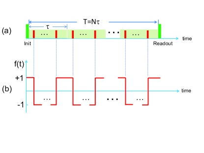
Figure 1: Quantum sensing by adaptive periodic quantum control. (a) The qubit is first initialized into the $\hat{\sigma}_{x}=+1$ eigenstate $|+\rangle$, and then experiences a periodic quantum control with $N$ identical control units of duration $\tau$. Each control unit consists of an even number of instantaneous $\pi$ pulses. Finally $\hat{\sigma}_{x}$ is readout by a projective measurement. (b) Modulation function of this periodic quantum control. The vertical dashed lines are guides to the eye.

We consider using a qubit as a quantum probe to sense the frequency $\omega$ of a harmonic oscillator that cannot be accessed directly. The Hamiltonian is the sum of the qubit term $\omega_{0}\hat{\sigma}_{z}/2$, the oscillator term $\omega\hat{b}^{\dagger}\hat{b}$, and the qubit-oscillator coupling $(\lambda/2)(\hat{b}^{\dagger}+\hat{b})\hat{\sigma}_{z}$ Neukirch et al. (2013); Scala et al. (2013); Zhao and Yin (2014), where $\hat{\sigma}_{x,y,z}$ are Pauli matrices for the qubit. This model has been realized experimentally in various hybrid quantum systems LaHaye et al. (2009); Hunger et al. (2010); Bennett et al. (2010); Arcizet et al. (2011); Kolkowitz et al. (2012b); YeoI. et al. (2014) by coupling a two-level system to a mechanical nano-oscillator Aspelmeyer et al. (2014). As shown in Fig. 1(a), the quantum control on the qubit consists of $N$ identical units of duration $\tau$ and each unit consists of an even number of $\pi$-pulses. Each $\pi$-pulse causes an instantaneous $\pi$-rotation $e^{-i(\pi/2)\hat{\sigma}_{x}}$ of the qubit around the $x$ axis. In the interaction picture of the qubit, the total Hamiltonian is

$$\mathcal{H}(t)=\omega\hat{b}^{\dagger}\hat{b}+f(t)\frac{\lambda}{2}(\hat{b}^{\dagger}+\hat{b})\hat{\sigma}_{z},$$

where $f(t)$ is the modulation function associated with the quantum control Yang et al. (2017): it starts from $f(0)=+1$ and changes its sign at the timings of each $\pi$-pulse [Fig. 1(b)]. Using the Wei-Norman algebra method Sun and Xiao (1991), the evolution operator during the total period $T\equiv N\tau$ of the quantum control is obtained as $\hat{U}=e^{-i\omega T\hat{b}^{\dagger}\hat{b}}\hat{D}(\hat{\sigma}_{z}\alpha)$, where $\hat{D}(z)=e^{z\hat{b}^{\dagger}-z^{\ast}\hat{b}}$ is the oscillator displacement operator and

$$\alpha=-i\frac{\lambda}{2}\int_{0}^{N\tau}f(t)e^{i\omega t}dt=\alpha_{1}K,$$

with $\alpha_{1}\equiv\alpha|_{N=1}$ for a single control unit and

$$K=\sum_{n=0}^{N-1}e^{i\omega n\tau}=\frac{e^{i\omega N\tau/2}}{e^{i\omega\tau/2}}\frac{\sin\frac{\omega N\tau}{2}}{\sin\frac{\omega\tau}{2}}$$

for the interference from $N$ control units.

Before the quantum control, we initialize the qubit into the $\hat{\sigma}_{x}=+1$ eigenstate $|+\rangle=(|\uparrow\rangle+|\downarrow\rangle)/\sqrt{2}$, but leave the oscillator in an arbitrary initial state $\hat{\rho}$ since the oscillator cannot be initialized. The evolution $\hat{U}$ during the quantum control drives the coupled system into an entangled final state $\hat{U}|+\rangle\langle+|\hat{\rho}\hat{U}^{\dagger}$. Since the oscillator cannot be measured, only the quantum Fisher information $\mathcal{F}$ contained in the reduced density matrix of the qubit, $\hat{\rho}_{\mathrm{p}}\equiv 1/2+\left(L|\uparrow\rangle\langle\downarrow|+h.c.\right)/2$, can be converted into the classical Fisher information $F$, where $L\equiv\langle\hat{D}(2\alpha)\rangle$ is the off-diagonal coherence of the qubit and $\left\langle\cdots\right\rangle\equiv\operatorname*{Tr}\hat{\rho}(\cdots)$ denotes the average over the initial state of the oscillator. Here we assume $\hat{\rho}$ commutes with $\hat{b}^{\dagger}\hat{b}$ and leave the generalization to an arbitrary $\hat{\rho}$ to the next section. In this case, $L$ is real and $\mathcal{F}=(\partial_{\omega}L)^{2}/(1-L^{2})$ Zhong et al. (2013). Let $\bar{n}\equiv\langle\hat{b}^{\dagger}\hat{b}\rangle$, when

$$\sqrt{2\bar{n}+1}\left|\alpha\right|\ll 1,$$ (3)

we obtain $L\approx 1-2(2\bar{n}+1)|\alpha|^{2}$ and hence $\mathcal{F}\approx 4(2\bar{n}+1)(\partial_{\omega}|\alpha|)^{2}$. At the end of the quantum control, a projective measurement of $\hat{\sigma}_{x}$ on the qubit yields an outcome randomly sampled from $\{+1,-1\}$ according to the probability $P(\pm 1|\omega)=(1\pm L)/2$ and the classical Fisher information contained in each outcome is obtained as $F=\mathcal{F}$. Such measurements are experimentally available in traditional nuclear magnetic resonance and electron spin resonance systems. The ultimate sensing precision follows from Eq. (1) as

$$\delta\omega=\frac{1}{\sqrt{\mathcal{F}}}=\frac{1}{2\sqrt{2\bar{n}+1}\left|(\partial_{\omega}|\alpha|)\right|}.$$ (4)

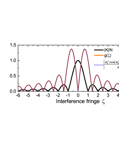
Figure 2: Interference fringes from periodic quantum control with $N=50$ control units. Here $\zeta\equiv N(\omega\tau/2\pi-1)$ labels the interference fringes near the major peak at $\omega\tau=2\pi$.

For large $N$, $|K|$ and hence $|\alpha|$ as functions of $\omega\tau$ exhibit many interference fringes with major peaks at integer multiples of $2\pi$. We focus on the major peak at $2\pi$ and label the surrounding interference fringes by $\zeta\equiv N\left(\omega\tau/2\pi-1\right)$, e.g., $\zeta=0$ labels the major peak and $\zeta=\pm 1,\pm 2$ labels the nodes (see the black solid line in Fig. 2). For $\left|\zeta\right|\ll N$, $\left|\alpha_{1}\right|$ is nearly a constant, so Eq. (9) simplifies to

$$\delta\omega\approx\frac{\pi}{g\tilde{\lambda}T^{2}},$$ (5)

where $\tilde{\lambda}\equiv\sqrt{2\bar{n}+1}\left|\alpha_{1}\right|/\tau$ is nearly a constant and $g(\zeta)\equiv|(\partial_{\zeta}|K|/N)|$ approaches a universal function (see Fig. 2)

$$g(\zeta)\approx\left|\frac{\pi\zeta\cos(\pi\zeta)-\sin(\pi\zeta)}{\pi\zeta^{2}}\right|\approx\left\{\begin{array}[c]{l}\frac{\pi^{2}\left|\zeta\right|}{3}e^{-(\pi\zeta)^{2}/10}\ (|\zeta|\ll 1),\\ \\ \frac{|\cos(\pi\zeta)|}{\left|\zeta\right|}\ \ \ \ \ (|\zeta|\gtrsim 1).\end{array}\right.$$

There are two tunable parameters: the duration $\tau$ of each control unit and the total number $N$ of control units. We set $\tau$ close to $2\pi/\omega$ to make $\zeta\approx 1$, so that $\left|\alpha\right|$ is sufficiently small to satisfy Eq. (3), while $g\approx 1$ is large to optimize the sensing precision. With $\tau$ largely fixed, we can increase the evolution time $T=N\tau$ by increasing $N$, so $\delta\omega\approx 1/(\tilde{\lambda}T^{2})$. Interestingly, this $1/T^{2}$ scaling originates from the interference between different control units: $\partial_{\omega}|K|\propto T^{2}$, while the internal structure of each control unit only affects the value of $\left|\alpha_{1}\right|/\tau$ and hence $\tilde{\lambda}$, e.g., $\left|\alpha_{1}\right|/\tau\approx\lambda/\pi$ for the Carr–Purcell–Meiboom–Gill sequence Carr and Purcell (1954); Meiboom and Gill (1958) with two $\pi$-pulses locate at $\tau/4$ and $3\tau/4$ in one control unit.

I.3 Origin of $1/T^{2}$ scaling

Compared with the previous work Yuan and Fung (2015); Yuan (2016) for sensing classical signals, where sophisticated feedback control are required to achieve the universal $1/T$ scaling, it is interesting that for the more challenging task – sensing quantum objects, our protocol can achieve the $1/T^{2}$ scaling by applying a simple periodic quantum control on the qubit without any direct access to the oscillator. The solution is that the previous derivation of the universal $1/T$ Yuan and Fung (2015); Yuan (2016) scaling for sensing classical signals assumes the quantum probe has a fixed and bounded spectrum. When this restriction is lifted, e.g., if the Hamiltonian itself increases with time $t$ as $\theta t^{k}\hat{H}$, then the precision $\delta\theta$ would be given by Eq. (2) with $H_{\mathrm{rms}}\rightarrow T^{k}\hat{H}_{\mathrm{rms}}$, i.e., $\delta\theta\propto 1/T^{k+1}$ Pang and Jordan (2017). By contrast, although sensing quantum objects suffers from the lack of direct access to the target, the spectrum of the target may be unbounded (even though the spectrum of the probe is bounded) and can further be manipulated indirectly via the probe, so the time scaling is not limited to $1/T$, but instead can be raised by engineering the evolution of the target, e.g., through the periodic driving on the qubit in our qubit-oscillator model. However, the lack of direct access to the target does lead to some surprising consequences, as we discuss now.

First, the condition Eq. (3) for achieving the $1/T^{2}$ scaling leads to $\hat{U}\approx e^{-i\omega T\hat{b}^{\dagger}\hat{b}}$, i.e., the final state of the coupled system at the end of the quantum control should largely coincide with their initial product state $|+\rangle\langle+|\otimes\hat{\rho}$. In other words, achieving the $1/T^{2}$ scaling requires neither appreciable probe-target entanglement nor appreciable energy fluctuation in the initial or final state of the coupled system, despite a large amount of energy exchange during the evolution. For example, even if the oscillator starts from (and ends up with) the lowest-energy vacuum state, we still obtain Eq. (5) (albeit with $\bar{n}=0$). This differs from sensing classical signals, where large scale entanglement and large energy fluctuation in the initial or final state are standard quantum resources to improve the precision Giovannetti et al. (2006), e.g., according to Eq. (2), to achieve optimal precision, the quantum system should start from (and end with) a highly excited state – an equal superposition of the highest eigenstate and the lowest eigenstate of $\hat{H}$.

Second, if we tune $\tau$ to make $|\alpha|\gg 1$, then the evolution $\hat{U}=e^{-i\omega T\hat{b}^{\dagger}\hat{b}}\hat{D}(\hat{\sigma}_{z}\alpha)$ would lead to large bifurcated displacement of the oscillator by $\pm\alpha$ for the qubit state being $|\uparrow\rangle$ or $|\downarrow\rangle$, so the final state of the coupled system is highly entangled. Although this state do contain a lot of quantum Fisher information about $\omega$, converting all of them into classical Fisher information would require projective measurements in the qubit-oscillator entangled basis, which is unavailable. The only object that can be measured is the final state of the qubit which, for $|\alpha|\gg 1$, is almost completely random and contains little quantum Fisher information about $\omega$. In other words, feeding a large amount of energies into the final state of the oscillator degrades, instead of improves, the sensing precision.

Third, thermal fluctuation of the oscillator usually degrades the sensing precision dramatically, e.g., if the initial state of the oscillator is a thermal state, then using the Linked-cluster expansion Yang et al. (2017) gives $L=e^{-2(2\bar{n}+1)|\alpha|^{2}}$, so $\mathcal{F}\sim(\partial_{\omega}L)^{2}$ is exponentially suppressed when $\sqrt{2\bar{n}+1}|\alpha|\gg 1$, similar to the case of measuring the frequency of a harmonic oscillator under classical driving by directly monitoring its positions. However, in our protocol, we can tune $\tau$ to make $|\alpha|$ sufficiently small so that Eq. (3) is satisfied, then $\mathcal{F}\propto\bar{n}$ and the sensing precision $\delta\omega\propto 1/\sqrt{\bar{n}}$ improves with $\bar{n}$ Zhao and Yin (2014).

In deriving Eqs. (9) and (5), we have assumed $[\hat{\rho},\hat{b}^{\dagger}\hat{b}]=0$ to make $L$ a real number. When this constraint is lifted, $L$ is in general complex, so $\mathcal{F}=|\partial_{\omega}L|^{2}+|L|^{2}(\partial_{\omega}|L|)^{2}/(1-|L|^{2})$ Zhong et al. (2013), where $L\approx 1+4i\operatorname{Im}\alpha\langle\hat{b}^{\dagger}\rangle+4\operatorname{Re}\alpha^{2}\langle b^{\dagger 2}\rangle-2(2\bar{n}+1)|\alpha|^{2}$ for small $|\alpha|$. As long as $\zeta=O(1)$, both $\partial_{\omega}\alpha$ and $\partial_{\omega}|\alpha|$ are of the order $T^{2}$, so we expect $\partial_{\omega}L,\partial_{\omega}|L|=O(T^{2})$ and $\mathcal{F}=O(T^{4})$, i.e., the $1/T^{2}$ scaling holds for a general oscillator initial state.

I.4 Adaptive quantum control

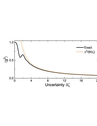
Figure 3: Performance of our protocol vs. uncertainty in tuning the interference fringes.

According to Eq. (5), the $1/T^{2}$ scaling can be achieved in two steps. First, we should tune $\tau$ to make $\zeta$ locate at the first node $\zeta=1$, so that $\left|\alpha\right|=0$ satisfies Eq. (3) and $g=1$. Second, we should increase $N$ to increase the total time $T$, so that $\delta\omega\approx\pi/(\tilde{\lambda}T^{2})$. However, our limited prior knowledge about $\omega$ – the unknown parameter – makes it impossible to make $\zeta$ locate at the first node precisely. If we our knowledge about $\omega$ has an uncertainty $\delta\omega$, then we would suffer from an uncertainty $\delta\zeta\equiv N\tau\delta\omega/2\pi$ in tuning the value of $\zeta$, so the achievable sensing precision is roughly given by Eq. (5) with $g(\zeta)$ replaced by $\langle g^{2}\rangle^{1/2}$, where $\langle g^{2}\rangle$ is the average of $g^{2}(\zeta)$ over the region $[1-\delta\zeta,1+\delta\zeta]$. As shown in Fig. 3, $\langle g^{2}\rangle\propto 1/\delta\zeta$ at large $\delta\zeta$, thus if $\delta\omega$ is fixed, then $\langle g^{2}\rangle\propto 1/N$ leads to $1/T^{3/2}$ scaling according to Eq. (5). To achieve the $1/T^{2}$ scaling, we need to ensure $\delta\zeta\lesssim 1$ and Eq. (3) simultaneously. This limits the $1/T^{2}$ scaling to

$$T\lesssim T_{\max}\equiv\sqrt{\frac{2\pi}{\delta\omega\max\{\delta\omega,\tilde{\lambda}\}}},$$ (6)

as determined by $\delta\omega$. This limitation can be lifted by using adaptive techniques.

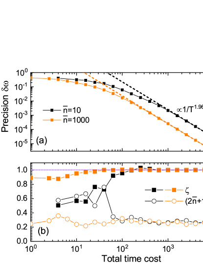
Figure 4: Numerical simulation of our protocol for a thermal initial state of the oscillator. (a) Sensing precision $\delta\omega$ vs. total time cost. (b) Evolution of $\zeta$ (squares) and $\sqrt{2\bar{n}+1}|\alpha|$ (circles) during the adaptive measurement. Each data is obtained by averaging the results of 500 repeated simulations. The dashed lines are linear fits to the simulation data. The true value of the frequency $\omega=50$, the thermal population $\bar{n}=10$ (black squares and circles) or $1000$ (orange squares and circles), the coupling strength $\lambda=0.1$, and the prior knowledge $\delta\omega_{0}=0.5$, and $\omega_{0}=50.5.$

Suppose before the sensing, we have an unbiased estimator $\omega_{0}$ with uncertainty $\tilde{\lambda}<\delta\omega_{0}\ll\omega_{0}$. This prior knowledge may come from preliminary measurements without quantum control. The entire scheme consists of many adaptive steps. The key idea is to utilize the knowledge acquired from the measurements in every step to reduce the uncertainty $\delta\omega$ in our knowledge about $\omega$, so that a longer evolution time $T$ can be used in the next step according to Eq. (6) (see Methods for details). In Fig. 4, we show the results from our numerical simulation for a thermal initial state of the oscillator. Figure 4(a) shows that (i) after a few tens of adaptive steps, the sensing precision begins to improve with the total time cost $\mathbb{T}$ according to the $1/\mathbb{T}^{2}$ scaling, where $\mathbb{T}$ can be extended indefinitely by increasing the number of adaptive steps; (ii) increasing the thermal fluctuation from $\bar{n}=10$ to $\bar{n}=1000$ improves the precision significantly. The onset of the $1/\mathbb{T}^{2}$ scaling can be understood from Fig. 4(b): after a few tens of adaptive steps, the value of $\zeta$ is tuned accurately to the first node $\zeta=1$ and Eq. (3) is well-satisfied.

II Discussions

To quantify the effect of the adaptive quantum control, we compare the sensing precision $\delta\omega\sim\pi/(\tilde{\lambda}\mathbb{T}^{2})$ under the quantum control to that without any control. The latter corresponds to $f(t)\equiv 1$ and hence $\left|\alpha\right|=(\lambda/\omega)\left|\sin(\omega\mathbb{T}/2)\right|$ for an evolution time $\mathbb{T}$, so the precision follows from Eq. (9) as $\delta\omega_{\mathrm{free}}\sim\omega/(\tilde{\lambda}\mathbb{T})$. Therefore, improving the precision from $\tilde{\lambda}$ to $\tilde{\lambda}/K$ requires a time cost $\mathbb{T}_{\mathrm{free}}\sim K\omega/\tilde{\lambda}^{2}$ without any control or $\mathbb{T}\sim\sqrt{K}/\tilde{\lambda}$ under the quantum control, i.e., the quantum control reduces the time cost by a factor

$$\frac{\mathbb{T}_{\mathrm{free}}}{\mathbb{T}}\sim\sqrt{K}\frac{\omega}{\tilde{\lambda}}\sim\sqrt{K}\frac{\omega}{\lambda}$$

that increases with increasing desired precision (i.e., increasing $K$) and decreasing coupling strength $\lambda$. In other words, our protocol is especially suited to high-precision sensing of remote quantum objects that are weakly coupled to the quantum probe – a most important yet challenging task.

In practice, the evolution time $T$ would be ultimately limited by the finite coherence time $T_{2}$ of the qubit , so the coherent evolution time $T=N\tau$ in each measurement would reach $T_{2}$ after some adaptive steps. Afterwards, the optimal strategy is to repeat the measurements with evolution time $T\sim T_{2}$ in all the subsequent steps, so the performance is quantified by the frequency sensitivity $\mathbb{S}\equiv\delta\omega\sqrt{T}$, which is $\mathbb{S}\sim\pi/(\tilde{\lambda}T_{2}^{3/2})$ under the quantum control and $\mathbb{S}_{\mathrm{free}}\sim\omega/(\tilde{\lambda}\sqrt{T_{2}})$ without any control. Therefore, the adaptive quantum control enhances the sensitivity by a factor

$$\frac{\mathbb{S}_{\mathrm{free}}}{\mathbb{S}}\sim\frac{\omega T_{2}}{\pi}.$$

For electron spin qubits in diamond nitrogen-vacancy center, the coherence time $T_{2}$ reaches a few milliseconds Gaebel et al. (2006); Takahashi et al. (2008); Balasubramanian et al. (2009); de Lange et al. (2010) at room temperature and even approaches one second at 77 K Bar-Gill et al. (2013). The experimentally demonstrated oscillator frequency $\omega$ ranges from kHz to GHz (see Ref. Aspelmeyer et al., 2014 for a review). For a rough estimate, we take $\omega/2\pi=100$ MHz and $T_{2}=1$ ms, which gives an enhancement $\mathbb{S}_{\mathrm{free}}/\mathbb{S}\sim 10^{5}$.

In summary, based on an exactly solvable qubit-oscillator model, we have demonstrated theoretically the possibility to qualitatively improve the time scaling of the sensing precision for the oscillator  frequency from $1/T$ to $1/T^{2}$ by applying adaptive periodic quantum control on the qubit, without any direct access (initialization, control, or measurement) to the oscillator. This improvement is applicable to a general initial states of the oscillator and does not require appreciable qubit-oscillator entanglement or net energy injection into the final state of the oscillator. This provides a paradigm in which adaptive, periodic quantum control and quantum backaction are utilized to steer the evolution of the target quantum object and improve the precision of realistic quantum sensing by several orders of magnitudes. Our study highlights a useful routine for high-precision quantum sensing of remote quantum objects weakly coupled to a single quantum probe.

III Methods

Here we outline the adaptive scheme that lifts the limitation Eq. (6). Further details can be found in the supplementary materials. The entire scheme consists of two stages: stage (i) and stage (ii).

Stage (i) corresponds to the uncertainty $\delta\omega$ satisfying $\omega_{0}\gg\delta\omega\gtrsim\tilde{\lambda}$. In this stage, the large uncertainty $\delta\omega$ only allows short evolution time $T$, so a single measurement only improves the precision slightly. In the first step, we set the evolution time to $T_{1}\sim 2\pi/\delta\omega_{0}$ and perform $\nu_{1}=c^{2}/G_{1}^{2}$ $(c$ is a constant controlling parameter and $G_{1}\sim\tilde{\lambda}/\delta\omega_{0}\ll 1$) repeated measurements to improve the precision from $\delta\omega_{0}$ to $\delta\omega_{1}\approx\delta\omega_{0}/\sqrt{1+c^{2}}$. In the second step, we increase the evolution time to $T_{2}\sim 2\pi/\delta\omega_{1}\approx\sqrt{1+c^{2}}T_{1}$ and perform $\nu_{2}\approx\nu_{1}/(1+c^{2})$ repeated measurements to improve the precision to $\delta\omega_{2}\approx\delta\omega_{1}/\sqrt{1+c^{2}}$, and so on, until the precision $\delta\omega$ becomes comparable or less than $\tilde{\lambda}$. We denote the final estimator of this state by $\omega_{\mathrm{i}}$ and its uncertainty by $\delta\omega_{\mathrm{i}}$. For $c\ll 1$, the total time cost of this stage is $T_{\mathrm{i}}\sim\delta\omega_{0}/\tilde{\lambda}^{2}$ for $c\ll 1$.

Stage (ii) corresponds to the uncertainty $\delta\omega\lesssim\tilde{\lambda},$ which allows long evolution time, so a single measurement can improve the precision signfiicantly. In the first step, we set the evolution time to $T_{1}=(1/\kappa)\sqrt{2\pi/(\tilde{\lambda}\delta\omega_{\mathrm{i}})}$, where $\kappa\gg 1$ is a control parameter. Then we perform $\nu$ repeated measurements to improve the precision to $\delta\omega_{1}\approx\delta\omega_{\mathrm{i}}/\sqrt{1+\nu\eta^{2}}$, where $\eta\approx 2/\kappa^{2}$. In the second step, we increase the evolution time to $T_{2}\approx(1+\nu\eta^{2})^{1/4}T_{1}$ and perform $\nu$ repeated measurements to improve the precision to $\delta\omega_{2}\approx\delta\omega_{1}/\sqrt{1+\nu\eta^{2}}$, and so on. At the end of the $m$th step, the total time cost is $T_{\mathrm{ii}}=\nu(T_{1}+\cdots+T_{m})$ and the final precision is $\delta\omega\approx\delta\omega_{\mathrm{i}}/(\sqrt{1+\nu\eta^{2}})^{m}$. For $\sqrt{\nu}\eta\ll 1$, we have

$$\delta\omega\approx\frac{16\pi}{\eta^{3}}\frac{1}{\tilde{\lambda}T_{\mathrm{ii}}^{2}}\sim\frac{1}{\tilde{\lambda}T_{\mathrm{ii}}^{2}}.$$

The total time cost of both stages is $\mathbb{T}\equiv T_{\mathrm{i}}+T_{\mathrm{ii}}$. When $\delta\omega_{0}$ is not too large compared with $\tilde{\lambda}$ and/or the desired final precision is high, we have $\mathbb{T}\approx T_{\mathrm{ii}}$, so the sensing precision follows $1/\mathbb{T}^{2}$ scaling with the total time cost.

Author contributions statement

N. Z. conceived the idea, Y. N. F. formulated the theories for vacuum initial state of the oscillator and Carr-Purcell-Meiboom-Gill control on the oscillator, W. Y. generalized the theories to arbitrary initial states and arbitrary periodic quantum controls. N. Z. and Y. N. F. wrote the first version of the paper. W. Y. wrote the final version. All authors discussed the results and commented on the manuscript.

Additional information

Competing financial interests: The authors declare no competing financial interests. Here we describe the adaptive quantum control scheme for quantum sensing and analyze its performance. Two kinds of resources can be utilized to improve the precision: repeated measurements (as quantified by the number $\nu$ of repetition) is a classical resource that improves the precision according to the classical scaling $\delta\omega\propto 1/\sqrt{\nu}$; while the evolution time $T$ is a quantum resource that improves the precision according to the quantum enhanced scaling $\delta\omega\propto 1/T^{2}$. When the total resource – the total time cost $\mathbb{T}$ – is fixed, it is desirable to spend more resources on $T$ instead of $\nu$. An extreme case is to spend all the time cost on the quantum resource, i.e., a single measurement $(\nu=1$) with the evolution time $T=\mathbb{T}$.

Appendix A Adaptive quantum control: analytical analysis

Recall that when

$$\sqrt{2\bar{n}+1}\left|\alpha\right|\ll 1,$$ (7)

we obtain the sensing precision

$$\delta\omega\approx\frac{\pi}{g(\zeta)\tilde{\lambda}T^{2}},$$

where $\tilde{\lambda}\equiv\sqrt{2\bar{n}+1}\left|\alpha_{1}\right|/\tau$ is nearly a constant and

$$g(\zeta)\approx\left|\frac{\pi\zeta\cos(\pi\zeta)-\sin(\pi\zeta)}{\pi\zeta^{2}}\right|$$

is a function of $\zeta\equiv N\left(\omega\tau/2\pi-1\right)$. Ideally, we should first set $\tau=(2\pi/\omega)(1+1/N)$ to make $\zeta=1$ and then increase $N$ to increase $T\equiv N\tau$. Setting $\zeta=1$ exactly not only makes $|\alpha|=0$ to satisfy Eq. (7), but also makes $g=1$ to achieve the sensing precision

$$\delta\omega(T)\approx\frac{\pi}{\tilde{\lambda}T^{2}}.$$ (8)

However, if our knowledge about $\omega$ has an uncertainty $\delta\omega$, then we suffer from an uncertainty $\delta\zeta\equiv(T/2\pi)\delta\omega$ in tuning the value of $\zeta$, i.e., we cannot set $\zeta=1$ exactly, but instead only make $\zeta\in[1-\delta\zeta,1+\delta\zeta]$. In this case, the actual sensing precision is roughly given by

$$\delta\omega_{\mathrm{i}}(T)\approx\dfrac{\pi}{g_{\mathrm{rms}}\tilde{\lambda}T^{2}},$$ (9)

where $g_{\mathrm{rms}}\equiv\sqrt{\langle g^{2}\rangle}$ and $\langle g^{2}\rangle$ is the average of $g^{2}(\zeta)$ over the region $[1-\delta\zeta,1+\delta\zeta]$. Since $\langle g^{2}\rangle\sim 1$ when $\delta\zeta\lesssim 1$ but $\langle g^{2}\rangle\propto 1/\delta\zeta$ when $\delta\zeta\gg 1$, to achieve the $1/T^{2}$ scaling, we should ensure both Eq. (7) and

$$\delta\zeta\lesssim 1.$$ (10)

In the following, we assume $\tilde{\lambda}\ll\omega$, which is typically the case in hybrid quantum systems.

In early stages of the sensing (i.e., $\delta\omega\gg\tilde{\lambda}$), Eq. (10) limits the coherent evolution time to $T\lesssim 2\pi/\delta\omega\ll 2\pi/\tilde{\lambda}$. Then, using $|K|\leq N$ gives $\sqrt{2\bar{n}+1}\left|\alpha\right|\leq\tilde{\lambda}T$, so Eq. (7) is satisfied automatically. Therefore, in the early stages of the sensing, we need only satisfy Eq. (10) by setting

$$T\approx\dfrac{1}{\kappa_{\mathrm{i}}}\dfrac{2\pi}{\delta\omega},$$ (11)

where $\kappa_{\mathrm{i}}\gtrsim 1$. In this case, we have $\delta\zeta\approx 1/\kappa_{\mathrm{i}}\lesssim 1$, so the sensing precision is given by Eq. (9).

As the sensing goes on, $\delta\omega$ becomes smaller than $\tilde{\lambda}$, then using $\tau\approx 2\pi/\omega$, we have $N\approx\omega T/(2\pi)\gg 1,$ so $\sqrt{2\bar{n}+1}|\alpha|\approx\tilde{\lambda}T\left|\sin(\pi\zeta)/(\pi\zeta)\right|\sim\tilde{\lambda}T\delta\zeta$, so Eq. (7) amounts to

$$\delta\zeta\ll\frac{1}{\tilde{\lambda}T}\Leftrightarrow T\ll\sqrt{\frac{2\pi}{\tilde{\lambda}\delta\omega}}.$$

To satisfy Eqs. (7) and (10) simultaneously, we set

$$T\approx\dfrac{1}{\kappa}\sqrt{\dfrac{2\pi}{\tilde{\lambda}\delta\omega}},$$ (12)

where $\kappa\gg 1$. Under this condition, we have $\delta\zeta=(1/\kappa)\sqrt{\delta\omega/(2\pi\tilde{\lambda})}\ll 1$, so the sensing precision is given by Eq. (8).

Next we describe the adaptive quantum sensing schemes capable of extending the $1/T^{2}$ scaling to arbitrarily long $T$. Before the quantum sensing, our prior knowledge about $\omega$ is quantified by a Gaussian distribution

$$P_{0}(\omega)=\frac{1}{\sqrt{2\pi}\delta\omega_{0}}e^{-(\omega-\omega_{0})^{2}/[2(\delta\omega_{0})^{2}]},$$ (13)

corresponding to an unbiased estimator $\omega_{0}$ with a precision (or uncertainty) $\tilde{\lambda}\ll\delta\omega_{0}\ll\omega$. The adaptive scheme consists of many steps. The central idea is to utilize the measurements in each step to successively refine our knowledge about $\omega$ and reduce the uncertainty $\delta\omega$, so that we can use successively longer coherent evolution time in the next step. The entire adaptive scheme consists of two stages: (i) $\delta\omega\gtrsim\tilde{\lambda}$, where we choose $T$ according to Eq. (11) to achieve Eq. (9); and (ii) $\delta\omega\lesssim\tilde{\lambda}$, where we choose $T$ according to Eq. (12) to achieve Eq. (8).

A.1 Stage (i): $\delta\omega\gtrsim\tilde{\lambda}$

In this stage, the large uncertainty $\delta\omega$ only allows short evolution times, so a single measurement only improves the precision slightly. Therefore, we need to utilize the classical resources (i.e., repeated measurements) to boost the improvement of the precision:

Step 1. We require the pulse interval $\tau_{1}$ and the pulse number $N_{1}$ to satisfy $\omega_{0}\tau_{1}-2\pi=2\pi/N_{1}$ and the evolution time $T_{1}\equiv N_{1}\tau_{1}$ to be close to $(1/\kappa_{\mathrm{i}})2\pi/\delta\omega_{0}$, where $\kappa_{\mathrm{i}}\gtrsim 1$ is a constant parameter. Then we repeat the projective $\hat{\sigma}_{x}$ measurements on the qubit for $\nu_{1}$ times and obtain the measurement outcomes $\mathbf{u}_{1}\equiv(u_{1},u_{2},\cdots,u_{\nu_{1}})$. Next we combine our prior knowledge and the new information from the outcomes $\mathbf{u}_{1}$ to update the distribution for $\omega$ from $P_{0}(\omega)$ to

$$P_{\mathbf{u}_{1}}(\omega)=\frac{P_{0}(\omega)P(\mathbf{u}_{1}|\omega)}{\int P_{0}(\omega)P(\mathbf{u}_{1}|\omega)d\omega},$$

where $P(\mathbf{u}_{1}|\omega)$ is the probability for obtaining the outcome $\mathbf{u}_{1}$. Then we construct the maximum likelihood estimator

$$\omega_{1}=\arg\max_{\omega}P_{\mathbf{u}_{1}}(\omega)$$

as the position of the maximum of $P_{\mathbf{u}_{1}}(\omega)$. For large $\nu_{1}$, the maximum likelihood estimator attains the Cramér-Rao bound, so its precision (or uncertainty) $\delta\omega_{1}$ is estimated by using the Cramér-Rao bound as

$$\delta\omega_{1}=\frac{1}{\sqrt{(\delta\omega_{0})^{-2}+\nu_{1}[\delta\omega_{\mathrm{i}}(T_{1})]^{-2}}}=\frac{\delta\omega_{0}}{\sqrt{1+\nu_{1}G_{1}^{2}}},$$

where

$$G_{1}\equiv\frac{\delta\omega_{0}}{\delta\omega_{\mathrm{i}}(T_{1})}\approx\eta_{\mathrm{i}}\frac{\tilde{\lambda}}{\delta\omega_{0}}$$

quantifies the information gain $\delta\omega_{\mathrm{i}}(T_{1})$ [Eq. (9)] from a single measurement relative to the prior knowledge $\delta\omega_{0}$ and

$$\eta_{\mathrm{i}}\equiv\frac{4\pi g_{\mathrm{rms}}}{\kappa_{\mathrm{i}}^{2}}\sim 1.$$ (14)

Initially $\delta\omega_{0}\gg\tilde{\lambda}$, so $G_{1}\ll 1$, i.e., a single measurement only improves the precision slightly. Then we have to utilize the classical resource $\nu_{1}\gg 1$ to boost the improvement of the precision. Taking $\nu_{1}=c_{\mathrm{i}}^{2}/G_{1}^{2}$ ($c_{\mathrm{i}}$ is a constant parameter) improves the precision by a factor $\sqrt{1+c_{\mathrm{i}}^{2}}$:

$$\delta\omega_{1}\approx\frac{\delta\omega_{0}}{\sqrt{1+c_{\mathrm{i}}^{2}}}.$$

The time cost of this step is

$$\nu_{1}T_{1}\approx\frac{c_{\mathrm{i}}^{2}\kappa_{\mathrm{i}}^{3}}{8\pi g_{\mathrm{rms}}^{2}}\frac{\delta\omega_{0}}{\tilde{\lambda}^{2}}.$$

Step 2. We require the pulse interval $\tau_{2}$ and the pulse number $N_{2}$ to satisfy $\omega_{1}\tau_{2}-2\pi=2\pi/N_{2}$ and the evolution time $T_{2}\equiv N_{2}\tau_{2}$ to be close to $(1/\kappa_{\mathrm{i}})2\pi/\delta\omega_{1}\approx\sqrt{1+c_{\mathrm{i}}^{2}}T_{1}$. Then we repeat the projective $\hat{\sigma}_{x}$ measurement on the qubit for $\nu_{2}$ times and obtain the measurement outcomes $\mathbf{u}_{2}\equiv(u_{1},u_{2},\cdots,u_{\nu_{2}})$. Next we combine our previous knowledge $P_{\mathbf{u}_{1}}(\omega)$ and the new information from the outcomes $\mathbf{u}_{2}$ to update the distribution for $\omega$ to

$$P_{\mathbf{u}_{1}\mathbf{u}_{2}}(\omega)=\frac{P_{\mathbf{u}_{1}}(\omega)P(\mathbf{u}_{2}|\omega)}{\int P_{\mathbf{u}_{1}}(\omega)P(\mathbf{u}_{2}|\omega)d\omega},$$

where $P(\mathbf{u}_{2}|\omega)$ is the probability for obtaining the outcome $\mathbf{u}_{2}$. Then we construct the maximum likelihood estimator $\omega_{2}$ as the position of the maximum of the probability distribution $P_{\mathbf{u}_{1}\mathbf{u}_{2}}(\omega)$. The precision (or uncertainty) $\delta\omega_{2}$ is estimated by the Cramér-Rao bound as

$$\delta\omega_{2}\approx\frac{1}{\sqrt{(\delta\omega_{1})^{-2}+\nu_{2}[\delta\omega_{\mathrm{i}}(T_{2})]^{-2}}}=\frac{\delta\omega_{1}}{\sqrt{1+\nu_{2}G_{2}^{2}}},$$

where the relative information gain

$$G_{2}\equiv\frac{\delta\omega_{1}}{\delta\omega_{\mathrm{i}}(T_{2})}\approx\eta_{\mathrm{i}}\frac{\tilde{\lambda}}{\delta\omega_{1}}\approx\sqrt{1+c_{\mathrm{i}}^{2}}G_{1}$$

is larger than the previous step due to the longer evolution time. Thus we need only utilize less classical resources $\nu_{2}=c_{\mathrm{i}}^{2}/G_{2}^{2}\approx\nu_{1}/(1+c_{\mathrm{i}}^{2})$ to improve the precision by the same factor $\sqrt{1+c_{\mathrm{i}}^{2}}$:

$$\delta\omega_{2}\approx\frac{\delta\omega_{1}}{\sqrt{1+c_{\mathrm{i}}^{2}}}.$$

The time cost of this step is $\nu_{2}T_{2}\approx\nu_{1}T_{1}/\sqrt{1+c_{\mathrm{i}}^{2}}$.

Step $m$. We require the pulse interval $\tau_{m}$ and the pulse number $N_{m}$ to satisfy $\omega_{m-1}\tau_{m}-2\pi=2\pi/N_{m}$ and the evolution time $T_{m}\equiv N_{m}\tau_{m}$ to be close to $(1/\kappa_{\mathrm{i}})2\pi/\delta\omega_{m-1}\approx\sqrt{1+c_{\mathrm{i}}^{2}}T_{m-1}$. Then we repeat the projective $\hat{\sigma}_{x}$ measurement on the qubit for $\nu_{m}$ times to obtain the maximum likelihood estimator $\omega_{m}$, whose precision is estimated as

$$\delta\omega_{m}\approx\frac{\delta\omega_{m-1}}{\sqrt{1+\nu_{m}G_{m}^{2}}},$$

where the relative information gain

$$G_{m}\equiv\frac{\delta\omega_{m-1}}{\delta\omega_{\mathrm{i}}(T_{m})}\approx\eta_{\mathrm{i}}\frac{\tilde{\lambda}}{\delta\omega_{m-1}}\approx\sqrt{1+c_{\mathrm{i}}^{2}}G_{m-1}.$$

As long as $\delta\omega_{m-1}\gg\tilde{\lambda}$, we have $G_{m}\ll 1$, so we still need to utilize the classical resource $\nu_{m}=c_{\mathrm{i}}^{2}/G_{m}^{2}\approx\nu_{m-1}/(1+c_{\mathrm{i}}^{2})$ to boost the improvement of the precision by a factor $\sqrt{1+c_{\mathrm{i}}^{2}}$:

$$\delta\omega_{m}\approx\frac{\delta\omega_{m-1}}{\sqrt{1+c_{\mathrm{i}}^{2}}}.$$

The time cost of this step is $\nu_{m}T_{m}\approx\nu_{m-1}T_{m-1}/\sqrt{1+c_{\mathrm{i}}^{2}}$.

This stage stops when the precision $\delta\omega$ becomes comparable or less than $\tilde{\lambda}$, so that a single measurement can lead to significant precision improvement.

In this stage, we have introduced two constant parameters $\kappa_{\mathrm{i}}$ and $c_{\mathrm{i}}$: the former ensures Eq. (10) is satisfied in every step, while the latter quantifies the classical resource to be utilized in each step. Every step improves the precision by a factor of $\sqrt{1+c_{\mathrm{i}}^{2}}$, but the time cost is $1/\sqrt{1+c_{\mathrm{i}}^{2}}$ times that of the previous step, consistent with the $1/T^{2}$ scaling of the sensing precision. The case $c_{\mathrm{i}}\gg 1$ corresponds to significant improvement of the precision in each step ($\delta\omega_{m}\ll\delta\omega_{m-1}$), so that the evolution time of the next step can be prolonged significantly ($T_{m}\gg T_{m-1}$); while $c_{\mathrm{i}}\ll 1$ corresponds to small improvement of the precision in each step ($\delta\omega_{m}\lesssim\delta\omega_{m-1}$), so that the evolution time of the next step can only be prolonged slightly ($T_{m}\gtrsim T_{m-1}$).

At the end of the $m$th step, the time cost is

$$T_{\mathrm{i}}\equiv\nu_{1}T_{1}+\cdots+\nu_{m}T_{m}\approx\nu_{1}T_{1}\frac{1-\frac{1}{(\sqrt{1+c_{\mathrm{i}}^{2}})^{m}}}{1-\frac{1}{\sqrt{1+c_{\mathrm{i}}^{2}}}}$$

and the precision is

$$\delta\omega_{m}\approx\frac{\delta\omega_{0}}{(\sqrt{1+c_{\mathrm{i}}^{2}})^{m}}.$$

For $c_{\mathrm{i}}\ll 1$ but large $m$ so that the overall precision improvement is significant, i.e., $(\sqrt{1+c_{\mathrm{i}}^{2}})^{m}\gg 1$, the time cost

$$T_{\mathrm{i}}\approx\frac{2\nu_{1}T_{1}}{c_{\mathrm{i}}^{2}}=\frac{\kappa_{\mathrm{i}}^{3}}{4\pi g_{\mathrm{rms}}^{2}}\frac{\delta\omega_{0}}{\tilde{\lambda}^{2}}$$

is independent of $c_{\mathrm{i}}$ and the number of steps $m$. When $c_{\mathrm{i}}\gg 1$, the time cost is dominated by the first step:

$$T_{\mathrm{i}}\approx\nu_{1}T_{1}\approx\frac{c_{\mathrm{i}}^{2}}{2}\frac{\kappa_{\mathrm{i}}^{3}}{4\pi g_{\mathrm{rms}}^{2}}\frac{\delta\omega_{0}}{\tilde{\lambda}^{2}}$$

and is still independent of $m$. The case $c_{\mathrm{i}}\ll 1$ requires less time cost than the case $c_{\mathrm{i}}\gg 1$, because the latter utilizes more classical resources (i.e., repeated measurements). On the other hand, in order to improve the precision from $\delta\omega_{0}$ to the desired precision $\tilde{\lambda}$, the case $c_{\mathrm{i}}\ll 1$ requires much more adaptive steps than the case $c_{\mathrm{i}}\gg 1$, because when $c_{\mathrm{i}}\ll 1$ ($c_{\mathrm{i}}\gg 1$), the precision is improved slightly (significantly) in each step.

A.2 Stage (ii): $\delta\omega\lesssim\tilde{\lambda}$

At the beginning of this stage, we have an estimator $\omega_{\mathrm{i}}$ (i.e., the estimator at the end of the previous stage) with a precision $\delta\omega_{\mathrm{i}}\sim\tilde{\lambda}$. In this stage, the small uncertainty $\delta\omega$ allows long evolution time so that a single measurement may significantly improve the precision.

Step 1. We require the pulse interval $\tau_{1}$ and the pulse number $N_{1}$ to satisfy $\omega_{\mathrm{i}}\tau_{1}-2\pi=2\pi/N_{1}$ and the evolution time $T_{1}\equiv N_{1}\tau_{1}$ to be close to $(1/\kappa)\sqrt{2\pi/(\tilde{\lambda}\delta\omega_{\mathrm{i}})}$, where $\kappa\gg 1$ is a constant parameter. Then we repeat the projective $\hat{\sigma}_{x}$ measurements on the qubit for $\nu$ times and construct the maximum likelihood estimator $\omega_{1}$. The precision of $\omega_{1}$ is estimated as

$$\delta\omega_{1}\approx\frac{\delta\omega_{\mathrm{i}}}{\sqrt{1+c^{2}}},$$

where $c\equiv\sqrt{\nu}\eta$,

$$\eta\equiv\frac{\delta\omega_{\mathrm{i}}}{\delta\omega(T_{1})}\approx\frac{2}{\kappa^{2}}$$ (15)

quantifies the relative information gain from a single measurement, and $\delta\omega(T_{1})$ is given by Eq. (8).

Step 2. We require the pulse interval $\tau_{2}$ and the pulse number $N_{2}$ to satisfy $\omega_{1}\tau_{2}-2\pi=2\pi/N_{2}$ and the evolution time $T_{2}\equiv N_{2}\tau_{2}$ to be close to $(1/\kappa)\sqrt{2\pi/(\tilde{\lambda}\delta\omega_{1})}\approx(1+c^{2})^{1/4}T_{1}$. Then we repeat the projective $\hat{\sigma}_{x}$ measurement on the qubit for $\nu$ times to obtain the maximum likelihood estimator $\omega_{2}$, whose precision is estimated as

$$\delta\omega_{2}\approx\frac{\delta\omega_{1}}{\sqrt{1+c^{2}}},$$

where we have used $\delta\omega_{1}/\delta\omega(T_{2})\approx\eta$.

Step $m$. We require the pulse interval $\tau_{2}$ and the pulse number $N_{2}$ to satisfy $\omega_{m-1}\tau_{m}-2\pi=2\pi/N_{m}$ and the evolution time $T_{m}\equiv N_{m}\tau_{m}$ to be close to $(1/\kappa)\sqrt{2\pi/(\tilde{\lambda}\delta\omega_{m-1})}\approx(1+c^{2})^{1/4}T_{m-1}$. Then we repeat the projective $\hat{\sigma}_{x}$ measurement on the qubit for $\nu$ times to obtain the maximum likelihood estimator $\omega_{m}$, whose precision is estimated as

$$\delta\omega_{m}\approx\frac{\delta\omega_{m-1}}{\sqrt{1+c^{2}}},$$

where we have used $\delta\omega_{m-1}/\delta\omega(T_{m})\approx\eta$.

In this stage, we have introduced two parameters $\kappa$ and $c$: the former ensures Eq. (7) is satisfied in every step, while the latter quantifies the classical resource to be utilized in each step. Every step improves the precision by a factor of $\sqrt{1+c^{2}}$ and uses a time cost that is $(1+c^{2})^{1/4}$ times that of the previous step, consistent with the $1/T^{2}$ scaling of the sensing precision. The case $c\gg 1$ corresponds to significant improvement of the precision in each step ($\delta\omega_{m}\ll\delta\omega_{m-1}$), so that the evolution time of the next step can be prolonged significantly ($T_{m}\gg T_{m-1}$); while the case $c\ll 1$ corresponds to small improvement of the precision in each step ($\delta\omega_{m}\lesssim\delta\omega_{m-1}$), so that the evolution time of the next step can only be prolonged slightly ($T_{m}\gtrsim T_{m-1}$).

At the end of the $m$th step, the time cost is

$$T_{\mathrm{ii}}=\nu(T_{1}+\cdots+T_{m})\approx\nu T_{1}\frac{(1+c^{2})^{m/4}-1}{(1+c^{2})^{1/4}-1},$$

and the final precision is

$$\delta\omega_{m}\approx\frac{\delta\omega_{\mathrm{i}}}{(\sqrt{1+c^{2}})^{m}}.$$

For $c\ll 1$, we have

$$\delta\omega_{m}\approx\frac{16}{\eta^{3}}\frac{\pi}{\tilde{\lambda}T_{\mathrm{ii}}^{2}}\approx 2\kappa^{6}\frac{\pi}{\tilde{\lambda}T_{\mathrm{ii}}^{2}}.$$

For $c\gg 1$, the total time cost is dominated by the last step: $T_{\mathrm{ii}}\approx\nu T_{m}$. The final precision is also dominated by the last step:

$$\delta\omega_{m}\approx\frac{\delta\omega(T_{m})}{\sqrt{\nu}}\approx\nu^{3/2}\frac{\pi}{\tilde{\lambda}T_{\mathrm{ii}}^{2}},$$ (16)

where $\delta\omega(T)$ is given in Eq. (8). Obviously, the case $c\ll 1$ provides better sensing precision than $c\gg 1$.

Appendix B Adaptive quantum control: numerical implementation

In our numerical simulation, we consider the $N$-period Carr–Purcell–Meiboom–Gill (CPMG) sequence consisting of $N$ identical control units $\tau/4$-$\pi$-$\tau/2$-$\pi$-$\tau/4$, corresponding to

$$\alpha_{1}(\omega,\tau)=i\frac{8\lambda}{\omega}e^{i\omega\tau/2}\cos\frac{\omega\tau}{8}\sin^{3}\frac{\omega\tau}{8}$$

and hence

$$\alpha(N,\omega,\tau)=\alpha_{1}(\omega,\tau)\sum_{n=0}^{N-1}e^{in\omega\tau}.$$

The initial state of the harmonic oscillator is taken as the thermal state $\rho=e^{-\omega a^{\dagger}a/(k_{B}T)}/\operatorname*{Tr}e^{-\omega a^{\dagger}a/(k_{B}T)}$, as characterized by the thermal population $\bar{n}=1/(e^{\omega/(k_{B}T)}-1)$. In this case, the off-diagonal coherence of the qubit is $L=e^{-2(2\bar{n}+1)|\alpha|^{2}}$ and the probability distribution of the $\sigma_{x}$ measurement is

$$P(\pm 1|\omega)=\frac{1\pm e^{-2(2\bar{n}+1)|\alpha|^{2}}}{2}.$$

B.1 Stage (i)

The input/control parameters include $\kappa_{\mathrm{i}}$, $c_{\mathrm{i}}$, $\bar{n}$, and the prior distribution $P_{0}(\omega)$ [Eq. (13)] for the unknown frequency $\omega$, as characterized by an estimator $\omega_{0}$ and its uncertainty $\delta\omega_{0}$.

At the beginning of the $k$-th adaptive step, we already have a probability distribution $P_{k-1}(\omega)$ from the previous steps, which gives an estimator $\omega_{k-1}$ and its uncertainty $\delta\omega_{k-1}$. In the $k$-th step, we apply the CPMG sequence with $N_{k}$ identical control units $\tau_{k}/4$-$\pi$-$\tau_{k}/2$-$\pi$-$\tau_{k}/4$ and repeat the measurements for $\nu_{k}$ times, where

$$N_{k} =\mathrm{nint}(\frac{\omega_{k-1}}{\kappa_{\mathrm{i}}\delta\omega_{k-1}}-1),$$ (17)

$$\tau_{k} =\frac{2\pi}{\omega_{k-1}}(1+\frac{1}{N_{k}}),$$ (18)

$$\nu_{k} =\max\{\mathrm{nint}\frac{c_{\mathrm{i}}^{2}(\delta\omega_{k-1})^{2}}{\tilde{\lambda}_{k}^{2}\eta_{\mathrm{i}}^{2}},1\},$$ (19)

with $\mathrm{nint}(a)$ for the integer closest to $a$, $\tilde{\lambda}_{k}\equiv\sqrt{2\bar{n}+1}|\alpha_{1}(\tau_{k},\omega_{k-1})|/\tau_{k}$, $\eta_{\mathrm{i}}$ given by Eq. (14), and $g_{\mathrm{rms}}\approx 0.83544$ is obtained by taking $\delta\zeta=1$. Next, we calculate $\alpha_{k}=\alpha(N_{k},\omega,\tau_{k})$ and $P_{k}(\pm 1|\omega)=(1\pm e^{-2(2\bar{n}+1)|\alpha_{k}|^{2}})/2$, randomly generate $\nu_{k}$ outcomes according to $P_{k}(\pm 1|\omega)$, and use $N_{\pm}$ to denote the number of outcome $\pm 1$ in those $\nu_{k}$ results. Then we calculate the updated probability distribution function

$$P_{k}(\omega)=P_{k-1}(\omega)[P_{k}(+1|\omega)]^{N_{+}}[P_{k}(-1|\omega)]^{N_{-}}$$

and obtain the maximum likelihood estimator $\omega_{k}\equiv\arg\max_{\omega}P_{k}(\omega)$ as the location of the maximum of $P_{k}(\omega)$ as a function of $\omega$. Finally, we calculate the uncertainty of $\omega_{k}$ by

$$\delta\omega_{k}=\left[\frac{\int d\omega(\omega_{k}-\omega)^{2}P_{k}(\omega)}{\int d\omega P_{k}(\omega)}\right]^{\frac{1}{2}}.$$

When $\delta\omega_{k}<\tilde{\lambda}_{k}$, this stage stops and we begin stage (ii) with

$$\omega_{\mathrm{i}} =\omega_{k},$$

$$\delta\omega_{\mathrm{i}} =\delta\omega_{k},$$

$$P_{\mathrm{i}}(\omega) =P_{k}(\omega).$$

B.2 Stage (ii)

The input/control parameters include $\kappa$, $c$, $\bar{n}$, and the distribution $P_{\mathrm{i}}(\omega)$, as characterized by an estimator $\omega_{\mathrm{i}}$ and its uncertainty $\delta\omega_{\mathrm{i}}$. At the beginning of the $k$-th adaptive step, we already have a probability distribution $P_{k-1}(\omega)$ from the previous steps, which gives an estimator $\omega_{k-1}$ and uncertainty $\delta\omega_{k-1}$. In the $k$-th adaptive step, we apply the CPMG sequence with $N_{k}$ identical control units $\tau_{k}/4$-$\pi$-$\tau_{k}/2$-$\pi$-$\tau_{k}/4$ and repeat the measurements for $\nu$ times, where

$$N_{k} =\mathrm{nint}(\frac{\omega_{k-1}}{\kappa\sqrt{2\pi\tilde{\lambda}\delta\omega_{k-1}}}-1),$$

$$\tau_{k} =\frac{2\pi}{\omega_{k-1}}(1+\frac{1}{N_{k}}),$$

$$\nu =\frac{c^{2}\kappa^{4}}{4},$$

and $\tilde{\lambda}=\lambda\sqrt{2\bar{n}+1}/\pi$. Next, we calculate $\alpha_{k}=\alpha(N_{k},\omega,\tau_{k})$ and $P_{k}(\pm 1|\omega)=(1\pm e^{-2(2\bar{n}+1)|\alpha_{k}|^{2}})/2$. Then we randomly generate $\nu$ outcomes according to $P_{k}(\pm 1|\omega)$, and let $N_{\pm}$ denote the number of outcome $\pm 1$ in those $\nu$ outcomes. Then we calculate the updated probability distribution function

$$P_{k}(\omega)=P_{k-1}(\omega)[P_{k}(+1|\omega)]^{N_{+}}[P_{k}(-1|\omega)]^{N_{-}}$$

and obtain the maximum likelihood estimator $\omega_{k}\equiv\arg\max_{\omega}P_{k}(\omega)$. Finally, we calculate the uncertainty of $\omega_{k}$ by

$$\delta\omega_{k}=\left[\frac{\int d\omega(\omega_{k}-\omega)^{2}P_{k}(\omega)}{\int d\omega P_{k}(\omega)}\right]^{\frac{1}{2}}.$$

This process can be continued until the uncertainty $\delta\omega_{k}$ reaches the desired precision.

In the numerical simulation, we take $\bar{n}=10$ and $\bar{n}=1000$, respectively, $\lambda=0.1$, $\delta\omega_{0}=0.5$, $\omega_{0}=50.5$, $\omega=50$, $c_{\mathrm{i}}=c=0.1$ and $\kappa_{\mathrm{i}}=\kappa=2.$ The total time cost is $\mathbb{T}=T_{\mathrm{i}}+T_{\mathrm{ii}}$.

References

- Taylor et al. (2008) J. M. Taylor, P. Cappellaro, L. Childress, L. Jiang, D. Budker, P. R. Hemmer, A. Yacoby, R. Walsworth, and M. D. Lukin, Nat. Phys. 4, 810 (2008).
- Balasubramanian et al. (2008) G. Balasubramanian, I. Y. Chan, R. Kolesov, M. Al-Hmoud, J. Tisler, C. Shin, C. Kim, A. Wojcik, P. R. Hemmer, A. Krueger, et al., Nature 455, 648 (2008).
- Maze et al. (2008) J. R. Maze, P. L. Stanwix, J. S. Hodges, S. Hong, J. M. Taylor, P. Cappellaro, L. Jiang, M. V. G. Dutt, E. Togan, A. S. Zibrov, et al., Nature 455, 644 (2008).
- Robledo et al. (2011) L. Robledo, L. Childress, H. Bernien, B. Hensen, P. F. A. Alkemade, and R. Hanson, Nature 477, 574 (2011).
- Togan et al. (2010) E. Togan, Y. Chu, A. S. Trifonov, L. Jiang, J. Maze, L. Childress, M. V. G. Dutt, A. S. Sorensen, P. R. Hemmer, A. S. Zibrov, et al., Nature 466, 730 (2010).
- Togan et al. (2011) E. Togan, Y. Chu, A. Imamoglu, and M. D. Lukin, Nature 478, 497 (2011).
- Maze et al. (2011) J. R. Maze, A. Gali, E. Togan, Y. Chu, A. Trifonov, E. Kaxiras, and M. D. Lukin, New J. Phys. 13, 025025 (2011).
- O’Brien et al. (2001) J. L. O’Brien, S. R. Schofield, M. Y. Simmons, R. G. Clark, A. S. Dzurak, N. J. Curson, B. E. Kane, N. S. McAlpine, M. E. Hawley, and G. W. Brown, Phys. Rev. B 64, 161401 (2001).
- Morello et al. (2010) A. Morello, J. J. Pla, F. A. Zwanenburg, K. W. Chan, K. Y. Tan, H. Huebl, M. Mottonen, C. D. Nugroho, C. Yang, J. A. van Donkelaar, et al., Nature 467, 687 (2010).
- Degen et al. (2017) C. L. Degen, F. Reinhard, and P. Cappellaro, Rev. Mod. Phys. 89, 035002 (2017).
- Zhao et al. (2011) N. Zhao, J.-L. Hu, S.-W. Ho, J. T. K. Wan, and R.-B. Liu, Nat. Nanotechnol. 6, 242 (2011).
- Zhao et al. (2012) N. Zhao, J. Honert, B. Schmid, M. Klas, J. Isoya, M. Markham, D. Twitchen, F. Jelezko, R.-B. Liu, H. Fedder, et al., Nat Nano 7, 657 (2012).
- Taminiau et al. (2012) T. H. Taminiau, J. J. T. Wagenaar, T. van der Sar, F. Jelezko, V. V. Dobrovitski, and R. Hanson, Phys. Rev. Lett. 109, 137602 (2012).
- Kolkowitz et al. (2012a) S. Kolkowitz, Q. P. Unterreithmeier, S. D. Bennett, and M. D. Lukin, Phys. Rev. Lett. 109, 137601 (2012a).
- Cai et al. (2013) J. Cai, F. Jelezko, M. B. Plenio, and A. Retzker, New J. Phys. 15, 013020 (2013).
- London et al. (2013) P. London, J. Scheuer, J.-M. Cai, I. Schwarz, A. Retzker, M. B. Plenio, M. Katagiri, T. Teraji, S. Koizumi, J. Isoya, et al., Phys. Rev. Lett. 111, 067601 (2013).
- Laraoui et al. (2013) A. Laraoui, F. Dolde, C. Burk, F. Reinhard, J. Wrachtrup, and C. A. Meriles, Nat. Commun. 4, 1651 (2013).
- Shi et al. (2014) F. Shi, X. Kong, P. Wang, F. Kong, N. Zhao, R.-B. Liu, and J. Du, Nat. Phys. 10, 21 (2014).
- Lang et al. (2015) J. E. Lang, R. B. Liu, and T. S. Monteiro, Phys. Rev. X 5, 041016 (2015).
- Boss et al. (2016) J. M. Boss, K. Chang, J. Armijo, K. Cujia, T. Rosskopf, J. R. Maze, and C. L. Degen, Phys. Rev. Lett. 116, 197601 (2016).
- Zaiser et al. (2016) S. Zaiser, T. Rendler, I. Jakobi, T. Wolf, S.-Y. Lee, S. Wagner, V. Bergholm, T. Schulte-Herbrüggen, P. Neumann, and J. Wrachtrup, Nat. Commun. 7, 12279 (2016).
- Ma and Liu (2016a) W.-L. Ma and R.-B. Liu, Phys. Rev. Applied 6, 054012 (2016a).
- Ma and Liu (2016b) W.-L. Ma and R.-B. Liu, Phys. Rev. Applied 6, 024019 (2016b).
- Shu et al. (2017) Z. Shu, Z. Zhang, Q. Cao, P. Yang, M. B. Plenio, C. Müller, J. Lang, N. Tomek, B. Naydenov, L. P. McGuinness, et al., Phys. Rev. A 96, 051402 (2017).
- Liu et al. (2017) H. Liu, M. B. Plenio, and J. Cai, Phys. Rev. Lett. 118, 200402 (2017).
- Yuan and Fung (2015) H. Yuan and C.-H. F. Fung, Phys. Rev. Lett. 115, 110401 (2015).
- Yuan (2016) H. Yuan, Phys. Rev. Lett. 117, 160801 (2016).
- Pang and Jordan (2017) S. Pang and A. N. Jordan, Nat. Commun. 8, 14695 (2017).
- Nusran et al. (2012) N. M. Nusran, M. U. Momeen, , and M. V. G. Dutt, Nat. Nanotechnol. 7, 109 (2012).
- Waldherr et al. (2012) G. Waldherr, J. Beck, P. Neumann, R. S. Said, M. Nitsche, M. L. Markham, D. J. Twitchen, J. Twamley, F. Jelezko, and J. Wrachtrup, Nat. Nanotechnol. 7, 105 (2012).
- Bonato et al. (2016) C. Bonato, M. S. Blok, H. T. Dinani, D. W. Berry, M. L. Markham, D. J. Twitchen, and R. Hanson, Nat. Nanotechnol. 11, 247 (2016).
- Schmitt et al. (2017) S. Schmitt, T. Gefen, F. M. Stürner, T. Unden, G. Wolff, C. Müller, J. Scheuer, B. Naydenov, M. Markham, S. Pezzagna, et al., Science 356, 832 (2017).
- Boss et al. (2017) J. M. Boss, K. S. Cujia, J. Zopes, and C. L. Degen, Science 356, 837 (2017).
- Aspelmeyer et al. (2014) M. Aspelmeyer, T. J. Kippenberg, and F. Marquardt, Rev. Mod. Phys. 86, 1391 (2014).
- Braunstein and Caves (1994) S. L. Braunstein and C. M. Caves, Phys. Rev. Lett. 72, 3439 (1994).
- Kay (1993) S. M. Kay, Fundamentals of Statistical Signal Processing: Estimation Theory (Prentice-Hall, 1993).
- Helstrom (1976) C. W. Helstrom, Quantum Detection and Estimation Theory (Academic press, New York, 1976).
- Giovannetti et al. (2006) V. Giovannetti, S. Lloyd, and L. Maccone, Phys. Rev. Lett. 96, 010401 (2006).
- Pang and Brun (2014) S. Pang and T. A. Brun, Phys. Rev. A 90, 022117 (2014).
- Liu et al. (2015) J. Liu, X.-X. Jing, and X. Wang, Sci. Rep. 5, 8565 (2015).
- Neukirch et al. (2013) L. P. Neukirch, J. Gieseler, R. Quidant, L. Novotny, and A. N. Vamivakas, Opt. Lett. 38, 2976 (2013).
- Scala et al. (2013) M. Scala, M. S. Kim, G. W. Morley, P. F. Barker, and S. Bose, Phys. Rev. Lett. 111, 180403 (2013).
- Zhao and Yin (2014) N. Zhao and Z. Q. Yin, Phys. Rev. A 90, 042118 (2014).
- LaHaye et al. (2009) M. D. LaHaye, J. Suh, P. M. Echternach, K. C. Schwab, and M. L. Roukes, Nature 459, 960 (2009).
- Hunger et al. (2010) D. Hunger, S. Camerer, T. W. Hänsch, D. König, J. P. Kotthaus, J. Reichel, and P. Treutlein, Phys. Rev. Lett. 104, 143002 (2010).
- Bennett et al. (2010) S. D. Bennett, L. Cockins, Y. Miyahara, P. Grütter, and A. A. Clerk, Phys. Rev. Lett. 104, 017203 (2010).
- Arcizet et al. (2011) O. Arcizet, V. Jacques, A. Siria, P. Poncharal, P. Vincent, and S. Seidelin, Nat. Phys. 7, 1 (2011).
- Kolkowitz et al. (2012b) S. Kolkowitz, a. C. Bleszynski Jayich, Q. Unterreithmeier, S. D. Bennett, P. Rabl, J. G. E. Harris, and M. D. Lukin, Science 335, 1603 (2012b).
- YeoI. et al. (2014) YeoI., de AssisP-L., GloppeA., Dupont-FerrierE., VerlotP., M. S., DupuyE., ClaudonJ., GerardJ-M., AuffevesA., et al., Nat Nano 9, 106 (2014).
- Yang et al. (2017) W. Yang, W.-L. Ma, and R.-B. Liu, Rep. Prog. Phys. 80, 016001 (2017).
- Sun and Xiao (1991) C.-P. Sun and Q. Xiao, Communications in Theoretical Physics 16, 359 (1991).
- Zhong et al. (2013) W. Zhong, Z. Sun, J. Ma, X. Wang, and F. Nori, Phys. Rev. A 87, 022337 (2013).
- Carr and Purcell (1954) H. Carr and E. M. Purcell, Phys. Rev. 94, 630 (1954).
- Meiboom and Gill (1958) S. Meiboom and D. Gill, Rev. Sci. Instrum. 29, 688 (1958).
- Note (1) Note1, here we consider using the quantum probe for high-precision sensing of a well-defined frequency of the target quantum object. This requires the coherence time of the target to be much longer than that of the quantum probe, otherwise the target frequency would be broadened by , making high-precision sensing impossible.
- Gaebel et al. (2006) T. Gaebel, M. Domhan, I. Popa, C. Wittmann, P. Neumann, F. Jelezko, J. R. Rabeau, N. Stavrias, A. D. Greentree, S. Prawer, et al., Nat. Phys. 2, 408 (2006).
- Takahashi et al. (2008) S. Takahashi, R. Hanson, J. van Tol, M. S. Sherwin, and D. D. Awschalom, Phys. Rev. Lett. 101, 047601 (2008).
- Balasubramanian et al. (2009) G. Balasubramanian, P. Neumann, D. Twitchen, M. Markham, R. Kolesov, N. Mizuochi, J. Isoya, J. Achard, J. Beck, J. Tissler, et al., Nat. Mater. 8, 383 (2009).
- de Lange et al. (2010) G. de Lange, Z. H. Wang, D. Riste, V. V. Dobrovitski, and R. Hanson, Science 330, 60 (2010).
- Bar-Gill et al. (2013) N. Bar-Gill, L. M. Pham, A. Jarmola, D. Budker, and R. L. Walsworth, Nat. Commun. 4, 1743 (2013).
Acknowledgements
We acknowledge Professor I. Cirac for the inspiring discussions on the physical understanding the scaling relation. We thank Professor H.-D. Yuan, S.-L. Luo, X.-G. Wang, and Doctor Y. Yao for fruitful suggestions and comments on the manuscript. N.Z. is supported by NKBRP (973 Program) 2014CB848700 and NSFC Nos. 11374032 and 11121403. W.Y. is supported by NSFC Nos. 11774021, 11274036, and 11322542. C.P.S. is supported by NSFC Nos. 11421063, 11534002, 11121403, the national key research and development program (Grant No. 2016YFA0301201), and the National 973 program (Grants No. 2012CB922104 and No. 2014CB921403). We acknowledge support by NSFC program for ’Scientific Research Center’ (Program No. U1530401).