Optimistic Mirror Descent in Saddle-Point Problems:
Going the Extra (Gradient) Mile

Abstract.

Owing to their connection with generative adversarial networks, saddle-point problems have recently attracted considerable interest in machine learning and beyond. By necessity, most theoretical guarantees revolve around convex-concave (or even linear) problems; however, making theoretical inroads towards efficient GAN training depends crucially on moving beyond this classic framework. To make piecemeal progress along these lines, we analyze the behavior of mirror descent (MD) in a class of non-monotone problems whose solutions coincide with those of a naturally associated variational inequality – a property which we call coherence. We first show that ordinary, “vanilla” MD converges under a strict version of this condition, but not otherwise; in particular, it may fail to converge even in bilinear models with a unique solution. We then show that this deficiency is mitigated by optimism: by taking an “extra-gradient” step, optimistic mirror descent (OMD) converges in all coherent problems. Our analysis generalizes and extends the results of Daskalakis et al. (2018) for optimistic gradient descent (OGD) in bilinear problems, and makes concrete headway for provable convergence beyond convex-concave games. We also provide stochastic analogues of these results, and we validate our analysis by numerical experiments in a wide array of GAN models (including Gaussian mixture models, and the CelebA and CIFAR-10 datasets).

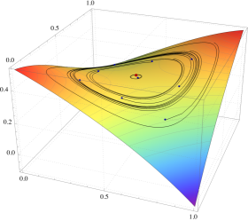
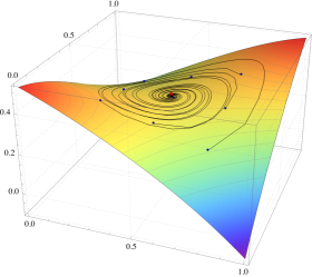
Figure 1. Mirror descent (MD) in the non-monotone saddle-point problem $f(x_{1},x_{2})=(x_{1}-1/2)(x_{2}-1/2)+\frac{1}{3}\exp(-(x_{1}-1/4)^{2}-(x_{2}-3/4)^{2})$. Left: vanilla MD spirals outwards; right: optimistic MD converges.

1. Introduction

The surge of recent breakthroughs in artificial intelligence (AI) has sparked significant interest in solving optimization problems that are universally considered hard. Accordingly, the need for an effective theory has two different sides: first, a deeper theoretical understanding would help demystify the reasons behind the success and/or failures of different training algorithms; second, theoretical advances can inspire effective algorithmic tweaks leading to concrete performance gains.

Deep learning has been an area of AI where theory has provided a significant boost. As a functional class, deep learning involves non-convex loss functions for which finding even local optima is NP-hard; nevertheless, elementary techniques such as gradient descent (and other first-order methods) seem to work fairly well in practice. For this class of problems, recent theoretical results have indeed provided useful insights: using tools from the theory of dynamical systems, Lee et al. (2016, 2017) and Panageas and Piliouras (2017) showed that a wide variety of first-order methods (including gradient descent and mirror descent) almost always avoid saddle points. More generally, the optimization and machine learning communities alike have dedicated significant effort in understanding the geometry of non-convex landscapes by searching for properties which could be leveraged for efficient training. For example, the well-known “strict saddle” property was shown to hold in a wide range of salient objective functions ranging from low-rank matrix factorization (Ge et al., 2016, 2017; Bhojanapalli et al., 2016) and dictionary learning (Sun et al., 2017b, a), to principal component analysis (Ge et al., 2015), phase retrieval (Sun et al., 2016), and many other models.

On the other hand, adversarial deep learning is nowhere near as well understood, especially in the case of GANs (Goodfellow et al., 2014). Despite an immense amount of recent scrutiny, our theoretical understanding cannot boast similar breakthroughs as in the case of “single-agent” deep learning. To make matters worse, GANs are notoriously hard to train and standard optimization methods often fail to converge to a reasonable solution. Because of this, a considerable corpus of work has been devoted to exploring and enhancing the stability of GANs, including techniques as diverse as the use of Wasserstein metrics (Arjovsky et al., 2017), critic gradient penalties (Gulrajani et al., 2017), different activation functions in different layers, feature matching, minibatch discrimination, etc. (Radford et al., 2015; Salimans et al., 2016).

A key observation in this context is that first-order methods may fail to converge even in toy, bilinear zero-sum games like Rock-Paper-Scissors and Matching Pennies (Piliouras and Shamma, 2014; Papadimitriou and Piliouras, 2016; Daskalakis et al., 2018; Mescheder et al., 2018; Mertikopoulos et al., 2018; Bailey and Piliouras, 2018). This is a critical failure of descent methods, but one which Daskalakis et al. (2018) showed can be overcome through “optimism”, interpreted in this context as a momentum adjustment that pushes the training process one step further along the incumbent gradient. In particular, Daskalakis et al. (2018) showed that OGD succeeds in cases where vanilla gradient descent (GD) fails (specifically, unconstrained bilinear saddle-point problems), and leveraged this theoretical result to improve the training of GANs.

A common theme in the above is that, to obtain a principled methodology for training GANs, it is beneficial to first establish improvements in a more restricted setting, and then test whether these gains carry over to more demanding learning environments. Following these theoretical breadcrumbs, we focus on a class of non-monotone problems whose solutions coincide with those of a naturally associated variational inequality, a property which we call coherence. Then, motivated by the success of mirror descent (MD) methods in online/stochastic convex programming, and hoping to overcome the shortcomings of ordinary gradient descent by exploiting the problem’s geometry, we examine the convergence of MD in coherent problems. On the positive side, we show that if a problem is strictly coherent (a condition that is satisfied by all strictly monotone problems), MD converges almost surely, even in stochastic problems (Theorem 3.1). However, under null coherence (the “saturated” opposite to strict coherence), MD spirals outwards from the problem’s solutions and may cycle in perpetuity, even with perfect gradient feedback. The null coherence property covers all bilinear models, so this result generalizes and extends the recent analysis of Daskalakis et al. (2018) and Bailey and Piliouras (2018) for gradient descent and follow-the-regularized-leader (FTRL) respectively (for a schematic illustration, see Figs. 1 and 5). Thus, in and by themselves, gradient/mirror descent methods do not suffice for training convoluted, adversarial deep learning models.

To mitigate this deficiency, we introduce an extra-gradient step which allows the algorithm to look ahead and take an “optimistic” mirror step along a “future” gradient. Following Rakhlin and Sridharan (2013), this method is known as optimistic mirror descent (OMD), and was first studied under the name “mirror-prox” by Nemirovski (2004). In convex-concave problems, Nemirovski (2004) showed that the so-called “ergodic average” of the algorithm’s iterates enjoys an $\operatorname{\mathcal{O}}(1/n)$ convergence rate. In the context of GAN training, Gidel et al. (2018) further introduced a “gradient reuse” mechanism to minimize the computational overhead of back-propagation and proved convergence in stochastic convex-concave problems. However, beyond the monotone regime, averaging offers no tangible benefits because Jensen’s inequality no longer applies; as a result, moving closer to GANs requires changing both the algorithm’s output structure as well as the accompanying analysis.

Our first result in this direction is that the last iterate of OMD converges in all coherent problems, including null-coherent ones. As a special case, this generalizes and extends the results of Daskalakis et al. (2018) for OGD in bilinear problems, and also settles in the affirmative an issue left open by the authors concerning the convergence of the algorithm in nonlinear problems. In addition, under the OMD algorithm, the (Bregman) distance to a solution decreases monotonically, so each iterate is better than the previous one (Theorem 4.1). Finally, under strict coherence, we also show that OMD converges with probability $1$ in stochastic saddle-point problems (Theorem 4.3). These results suggest that a straightforward, extra-gradient add-on can lead to significant performance gains when applied to existing state-of-the-art first-order methods (such as Adam). This theoretical prediction is validated experimentally in a wide array of GAN models (including Gaussian mixture models, and the CelebA and CIFAR-10 datasets) in Section 5.

2. Problem setup and preliminaries

Saddle-point problems.

Consider a saddle-point problem of the general form

$$\min_{x_{1}\in\mathcal{X}_{1}}\max_{x_{2}\in\mathcal{X}_{2}}f(x_{1},x_{2}),$$ (SP)

where each feasible region $\mathcal{X}_{i}$, $i=1,2$, is a compact convex subset of a finite-dimensional normed space $\mathcal{V}_{i}\equiv\mathbb{R}^{d_{i}}$, and $f\colon\mathcal{X}\equiv\mathcal{X}_{1}\times\mathcal{X}_{2}\to\mathbb{R}$ denotes the problem’s value function. From a game-theoretic standpoint, (SP) can be seen as a zero-sum game between two optimizing agents (or players): Player $1$ (the minimizer) seeks to incur the least possible loss, while Player $2$ (the maximizer) seeks to obtain the highest possible reward – both given by $f(x_{1},x_{2})$.

To obtain a solution of (SP), we will focus on incremental processes that exploit the individual loss/reward gradients of $f$ (assumed throughout to be at least $C^{1}$-smooth). Since the individual gradients of $f$ will play a key role in our analysis, we will encode them in a single vector as

$$g(x)=(g_{1}(x),g_{2}(x))=(\nabla_{x_{1}}f(x_{1},x_{2}),-\nabla_{x_{2}}f(x_{1},x_{2})),$$ (2.1)

and, following standard conventions, we will treat $g(x)$ as an element of $\mathcal{Y}\equiv\mathcal{V}^{\ast}$, the dual of the ambient space $\mathcal{V}\equiv\mathcal{V}_{1}\times\mathcal{V}_{2}$, assumed to be endowed with the product norm $\lVert x\rVert^{2}=\lVert x_{1}\rVert^{2}+\lVert x_{2}\rVert^{2}$.

Variational inequalities and coherence.

Most of the literature on saddle-point problems has focused on the monotone case, i.e., when $f$ is convex-concave. In such problems, it is well known that solutions of (SP) can be characterized equivalently as solutions of the associated (Minty) variational inequality:

$$\langle g(x),x-x^{\ast}\rangle\geq 0\quad\text{for all $x\in\mathcal{X}$}.$$ (VI)

Importantly, this equivalence extends well beyond the realm of monotone problems: it trivially includes all bilinear problems ($f(x_{1},x_{2})=x_{1}^{\top}Mx_{2}$), quasi-convex-concave objectives (where Sion’s minmax theorem applies), etc. For a concrete non-monotone example, consider the problem

$$\min_{x_{1}\in[-1,1]}\max_{x_{2}\in[-1,1]}(x_{1}^{4}x_{2}^{2}+x_{1}^{2}+1)(x_{1}^{2}x_{2}^{4}-x_{2}^{2}+1).$$ (2.2)

The only saddle-point of $f$ is $x^{\ast}=(0,0)$: it is easy to check that $x^{\ast}$ is also the unique solution of the corresponding problem (VI), despite the fact that $f$ is not even (quasi-)monotone. This shows that the equivalence between (SP) and (VI) encompasses a wide range of phenomena that are innately incompatible with convexity/monotonicity, even in the lowest possible dimension; for an in-depth discussion of the links between (SP) and (VI), we refer the reader to Facchinei and Pang (2003).

Motivated by this equivalence, we introduce below the notion of coherence:

Definition 2.1.

We say that (SP) is coherent if every saddle-point of $f$ is a solution of the associated variational inequality problem (VI) and vice versa. If (VI) holds as a strict inequality whenever $x$ is not a saddle-point of $f$, (SP) will be called strictly coherent; by contrast, if (VI) holds as an equality for all $x\in\mathcal{X}$, we will say that (SP) is null-coherent.

The notion of coherence will play a central part in our considerations, so a few remarks are in order. First, to the best of our knowledge, its first antecedent is a gradient condition examined by Bottou (1998) in the context of nonlinear programming; we borrow the term “coherence” from the more recent paper of Zhou et al. (2017) (who actually used the term to describe strict coherence). We should also note that it is possible to relax the equivalence between (SP) and (VI) by positing that only some of the solutions of (SP) can be harvested from (VI). Our analysis still goes through in this case but, to keep things simple, we do not pursue this relaxation here.

Finally, regarding the distinction between coherence and strict coherence, we show in Appendix A that (SP) is strictly coherent when $f$ is strictly convex-concave. At the other end of the spectrum, typical examples of problems that are null-coherent are bilinear objectives with an interior solution: for instance, $f(x_{1},x_{2})=x_{1}x_{2}$ with $x_{1},x_{2}\in[-1,1]$ has $\langle g(x),x\rangle=x_{1}x_{2}-x_{2}x_{1}=0$ for all $x_{1},x_{2}\in[-1,1]$, so it is null-coherent. Finally, neither strict, nor null coherence imply a unique solution to (SP), a property which is particularly relevant for GANs.

3. Mirror descent

The method.

Motivated by its prolific success in convex programming, our starting point will be the well-known mirror descent (MD) method of Nemirovski and Yudin (1983), suitably adapted to our saddle-point context; for a survey, see Hazan (2012) and Bubeck (2015).

The basic idea of mirror descent is to generate a new state variable $x^{+}$ from some starting state $x$ by taking a “mirror step” along a gradient-like vector $y$. To do this, let $h\colon\mathcal{X}\to\mathbb{R}$ be a continuous and $K$-strongly convex distance-generating function (DGF) on $\mathcal{X}$, i.e.,

$$h(tx+(1-t)x^{\prime})\leq th(x)+(1-t)h(x^{\prime})-\frac{1}{2}Kt(1-t)\lVert x^{\prime}-x\rVert^{2},$$ (3.1)

for all $x,x^{\prime}\in\mathcal{X}$ and all $t\in[0,1]$. In terms of smoothness (and in a slight abuse of notation), we also assume that the subdifferential of $h$ admits a continuous selection, i.e., a continuous function $\nabla h\colon\operatorname{dom}\partial h\to\mathcal{Y}$ such that $\nabla h(x)\in\partial h(x)$ for all $x\in\operatorname{dom}\partial h$. Then, following Bregman (1967), $h$ generates a pseudo-distance on $\mathcal{X}$ via the relation

$$D(p,x)=h(p)-h(x)-\langle\nabla h(x),p-x\rangle\quad\text{for all $p\in\mathcal{X}$, $x\in\operatorname{dom}\partial h$}.$$ (3.2)

This pseudo-distance is known as the Bregman divergence. As we show in Appendix B, we have $D(p,x)\geq\frac{1}{2}K\lVert x-p\rVert^{2}$, so the convergence of a sequence $X_{n}$ to some target point $p$ can be verified by showing that $D(p,X_{n})\to 0$. On the other hand, $D(p,x)$ typically fais to be symmetric and/or satisfy the triangle inequality, so it is not a true distance function per se. Moreover, the level sets of $D(p,x)$ may fail to form a neighborhood basis of $p$, so the convergence of $X_{n}$ to $p$ does not necessarily imply that $D(p,X_{n})\to 0$; we provide an example of this behavior in Appendix B. For technical reasons, it will be convenient to assume that such phenomena do not occur, i.e., that $D(p,X_{n})\to 0$ whenever $X_{n}\to p$. This mild regularity condition is known in the literature as “Bregman reciprocity” (Chen and Teboulle, 1993; Kiwiel, 1997), and it will be our standing assumption in what follows (note also that it holds trivially for both Examples 3.1 and 3.2 below).

Now, as with standard Euclidean distances, the Bregman divergence generates an associated prox-mapping defined as

$$P_{x}(y)=\operatorname*{arg\,min}_{x^{\prime}\in\mathcal{X}}\{\langle y,x-x^{\prime}\rangle+D(x^{\prime},x)\}\quad\text{for all $x\in\operatorname{dom}\partial h$, $y\in\mathcal{Y}$}.$$ (3.3)

In analogy with the Euclidean case (discussed below), the prox-mapping (3.3) produces a feasible point $x^{+}=P_{x}(y)$ by starting from $x\in\operatorname{dom}\partial h$ and taking a step along a dual (gradient-like) vector $y\in\mathcal{Y}$. In this way, we obtain the mirror descent (MD) algorithm

$$X_{n+1}=P_{X_{n}}(-\gamma_{n}\hat{g}_{n}),$$ (MD)

where $\gamma_{n}$ is a variable step-size sequence and $\hat{g}_{n}$ is the calculated value of the gradient vector $g(X_{n})$ at the $n$-th stage of the algorithm (for a pseudocode implementation, see Algorithm 1).

1:$K$-strongly convex regularizer $h\colon\mathcal{X}\to\mathbb{R}$, step-size sequence $\gamma_{n}>0$

2:choose $X\in\operatorname{dom}\partial h$ # initialization

3:for $n=1,2,\dotsc$ do

4:    oracle query at $X$ returns $g$ # gradient feedback

5:    set $X\leftarrow P_{X}(-\gamma_{n}g)$ # new state

6:end for

7:return $X$

Algorithm 1 mirror descent (MD) for saddle-point problems

For concreteness, two widely used examples of prox-mappings are as follows:

Example 3.1 (Euclidean projections).

When $\mathcal{X}$ is endowed with the $L^{2}$ norm $\lVert\cdot\rVert_{2}$, the archetypal prox-function is the (square of the) norm itself, i.e., $h(x)=\frac{1}{2}\lVert x\rVert_{2}^{2}$. In that case, $D(p,x)=\frac{1}{2}\lVert x-p\rVert^{2}$ and the induced prox-mapping is

$$P_{x}(y)=\operatorname{\Pi}(x+y),$$ (3.4)

with $\operatorname{\Pi}(x)=\operatorname*{arg\,min}_{x^{\prime}\in\mathcal{X}}\lVert x^{\prime}-x\rVert^{2}$ denoting the ordinary Euclidean projection onto $\mathcal{X}$.

Example 3.2 (Entropic regularization).

When $\mathcal{X}$ is a $d$-dimensional simplex, a widely used distance-generating function (DGF) is the (negative) Gibbs–Shannon entropy $h(x)=\sum_{j=1}^{d}x_{j}\log x_{j}$. This function is $1$-strongly convex with respect to the $L^{1}$ norm (Shalev-Shwartz, 2011) and the associated pseudo-distance is the Kullback–Leibler divergence $D_{\mathrm{KL}}(p,x)=\sum_{j=1}^{d}p_{j}\log(p_{j}/x_{j});$ in turn, this yields the prox-mapping

$$P_{x}(y)=\frac{(x_{j}\exp(y_{j}))_{j=1}^{d}}{\sum_{j=1}^{d}x_{j}\exp(y_{j})}\quad\text{for all $x\in\mathcal{X}^{\circ}$, $y\in\mathcal{Y}$.}$$ (3.5)

The update rule $x\leftarrow P_{x}(y)$ is known in the literature as the multiplicative weights (MW) algorithm (Arora et al., 2012), and is one of the centerpieces for learning in zero-sum games (Freund and Schapire, 1999; Mertikopoulos et al., 2018; Daskalakis et al., 2018), adversarial bandits (Auer et al., 1995), etc.

Regarding the gradient input sequence $\hat{g}_{n}$ of (MD), we assume that it is obtained by querying a first-order oracle which outputs an estimate of $g(X_{n})$ when called at $X_{n}$. This oracle could be either perfect, returning $\hat{g}_{n}=g(X_{n})$ for all $n$, or imperfect, providing noisy gradient estimations. By that token, we will make the following blanket assumptions for the gradient feedback sequence $\hat{g}_{n}$:

$$a)\;\textit{Unbiasedness:} \operatorname{\mathbb{E}}[\hat{g}_{n}\nonscript\,|\nonscript\,\mathopen{}\mathcal{F}_{n}]=g(X_{n}).$$ (3.6)

$$b)\;\textit{Finite mean square:} \operatorname{\mathbb{E}}[\lVert\hat{g}_{n}\rVert_{\ast}^{2}\nonscript\,|\nonscript\,\mathopen{}\mathcal{F}_{n}]\leq G^{2}\;\;\text{for some finite $G\geq 0$}.\hskip 80.00012pt$$

In the above, $\lVert y\rVert_{\ast}\equiv\sup\{\langle y,x\rangle:x\in\mathcal{V},\lVert x\rVert\leq 1\}$ denotes the dual norm on $\mathcal{Y}$ while $\mathcal{F}_{n}$ represents the history (natural filtration) of the generating sequence $X_{n}$ up to stage $n$ (inclusive). Since $\hat{g}_{n}$ is generated randomly from $X_{n}$ at stage $n$, it is obviously not $\mathcal{F}_{n}$-measurable, i.e., $\hat{g}_{n}=g(X_{n})+U_{n+1},$ where $U_{n}$ is an adapted martingale difference sequence with $\operatorname{\mathbb{E}}[\lVert U_{n+1}\rVert_{\ast}^{2}\nonscript\,|\nonscript\,\mathopen{}\mathcal{F}_{n}]\leq\sigma^{2}$ for some finite $\sigma\geq 0$. Clearly, when $\sigma=0$, we recover the exact gradient feedback framework $\hat{g}_{n}=g(X_{n})$.

Convergence analysis.

When (SP) is convex-concave, it is customary to take as the output of (MD) the so-called ergodic average

$$\bar{X}_{n}=\frac{\sum_{k=1}^{n}\gamma_{k}X_{k}}{\sum_{k=1}^{n}\gamma_{k}},$$ (3.7)

or some other average of the sequence $X_{n}$ where the objective is sampled. The reason for this is that convexity guarantees – via Jensen’s inequality and gradient monotonicity – that a regret-based analysis of (MD) can lead to explicit rates for the convergence of $\bar{X}_{n}$ to the solution set of (SP) (Nemirovski, 2004; Nesterov, 2007). Beyond convex-concave problems however, this is no longer the case: averaging provides no tangible benefits in a non-monotone setting, so we need to examine the convergence properties of the generating sequence $X_{n}$ of (MD) directly. With all this in mind, our main result for (MD) may be stated is as follows:

Theorem 3.1.

Suppose that (MD) is run with a gradient oracle satisfying (3.6) and a variable step-size sequence $\gamma_{n}$ such that $\sum_{n=1}^{\infty}\gamma_{n}=\infty$. Then:

1. If $f$ is strictly coherent and $\sum_{n=1}^{\infty}\gamma_{n}^{2}<\infty$, $X_{n}$ converges (a.s.) to a solution of (SP).

2. If $f$ is null-coherent, the sequence $\operatorname{\mathbb{E}}[D(x^{\ast},X_{n})]$ is non-decreasing for every solution $x^{\ast}$ of (SP).

This result establishes an important dichotomy between strict and null coherence: in strictly coherent problems, $X_{n}$ is attracted to the solution set of (SP); in null-coherent problems, $X_{n}$ drifts away and cycles without converging. In particular, this dichotomy leads to the following immediate corollaries:

Corollary 3.2.

Suppose that $f$ is strictly convex-concave. Then, with assumptions as above, $X_{n}$ converges (a.s.) to the (necessarily unique) solution of (SP).

Corollary 3.3.

Suppose that $f$ is bilinear and admits an interior saddle-point $x^{\ast}\in\mathcal{X}^{\circ}$. If $X_{1}\neq x^{\ast}$ and (MD) is run with exact gradient input ($\sigma=0$), we have $\lim_{n\to\infty}D(x^{\ast},X_{n})>0$.

Since bilinear models include all finite two-player, zero-sum games, Corollary 3.3 encapsulates both the non-convergence results of Daskalakis et al. (2018) and Bailey and Piliouras (2018) for gradient descent and FTRL respectively (for a more comprehensive formulation, see Proposition C.3 in Appendix C). This failure of (MD) is due to the fact that, witout a mitigating mechanism in place, a “blind” first-order step could overshoot and lead to an outwards spiral, even with a vanishing step-size. This phenomenon becomes even more pronounced in GANs where it can lead to mode collapse and/or cycles between different modes. The next two sections address precisely these issues.

4. Optimistic mirror descent

The method.

In convex-concave problems, taking an average of the algorithm’s generated samples as in (3.7) may resolve cycling phenomena by inducing an auxiliary sequence that gravitates towards the “center of mass” of the driving sequence $X_{n}$ (which orbits interior solutions). However, this technique cannot be employed in non-monotone problems because Jensen’s inequality does not hold there. In view of this, we replace averaging with an optimistic “extra-gradient” step which uses the obtained information to “amortize” the next prox step (possibly outside the convex hull of generated states). The seed of this “extra-gradient” idea dates back to Korpelevich (1976) and Nemirovski (2004), and has since found wide applications in optimization theory and beyond – for a survey, see Bubeck (2015) and references therein.

In a nutshell, given a state $x$, the extra-gradient method first generates an intermediate, “waiting” state $\hat{x}=P_{x}(-\gamma g(x))$ by taking a prox step as usual. However, instead of continuing from $\hat{x}$, the method samples $g(\hat{x})$ and goes back to the original state $x$ in order to generate a new state $x^{+}=P_{x}(-\gamma g(\hat{x}))$. Based on this heuristic, we obtain the optimistic mirror descent (OMD) algorithm

$$X_{n+1/2} =P_{X_{n}}(-\gamma_{n}\hat{g}_{n})$$ (OMD)

$$X_{n+1} =P_{X_{n}}(-\gamma_{n}\hat{g}_{n+1/2})$$

where, in obvious notation, $\hat{g}_{n}$ and $\hat{g}_{n+1/2}$ represent gradient oracle queries at the incumbent and intermediate states $X_{n}$ and $X_{n+1/2}$ respectively (for a pseudocode implementation, see Algorithm 2).

Algorithm 2 optimistic mirror descent (OMD) for saddle-point problems

1:$K$-strongly convex regularizer $h\colon\mathcal{X}\to\mathbb{R}$, step-size sequence $\gamma_{n}>0$

2:choose $X\in\operatorname{dom}\partial h$ # initialization

3:for $n=1,2,\dotsc$ do

4:    oracle query at $X$ returns $g$ # gradient feedback

5:    set $X^{+}\leftarrow P_{X}(-\gamma_{n}g)$ # waiting state

6:    oracle query at $X^{+}$ returns $g^{+}$ # gradient feedback

7:    set $X\leftarrow P_{X}(-\gamma_{n}g^{+})$ # new state

8:end for

9:return $X$

Convergence analysis.

In his original analysis, Nemirovski (2004) considered the ergodic average (3.7) of the algorithm’s iterates and established an $\operatorname{\mathcal{O}}(1/n)$ convergence rate in monotone problems. However, as we explained above, even though this kind of averaging is helpful in convex-concave problems, it does not provide any tangible benefits beyond this class: in more general problems, $X_{n}$ appears to be the most natural solution candidate. Our first result below justifies this choice in the class of coherent problems:

Theorem 4.1.

Suppose that (SP) is coherent and $g$ is $L$-Lipschitz continuous. If (OMD) is run with exact gradient input ($\sigma=0$) and $\gamma_{n}$ such that $0<\inf_{n}\gamma_{n}\leq\sup_{n}\gamma_{n}<K/L,$ the sequence $X_{n}$ converges monotonically to a solution $x^{\ast}$ of (SP), i.e., $D(x^{\ast},X_{n})$ decreases monotonically to $0$.

Corollary 4.2.

Suppose that $f$ is bilinear. If (OMD) is run with assumptions as above, the sequence $X_{n}$ converges monotonically to a solution of (SP).

Theorem 4.1 includes as a special case the analysis of Facchinei and Pang (2003, Theorem 12.1.11) for optimistic gradient descent and, in turn, the corresponding asymptotic result of Daskalakis et al. (2018) for bilinear saddle-point problems. As in the case of Daskalakis et al. (2018), Theorem 4.1 shows that optimism (i.e., the extra-gradient add-on) plays a crucial role in stabilizing (MD): not only does (OMD) converge in problems where (MD) provably fails (e.g., in zero-sum finite games), but this convergence is, in fact, monotonic. In other words, at each iteration, (OMD) comes closer to a solution of (SP), whereas (MD) may spiral outwards, towards higher and higher values of the Bregman divergence, ultimately converging to a limit cycle. This phenomenon can be seen very clearly in Fig. 1, and also in the detailed analysis we provide in Appendix C.

Of course, except for very special cases, the monotonic convergence of $X_{n}$ cannot hold when the gradient input to (OMD) is imperfect: a single “bad” sample of $\hat{g}_{n}$ would suffice to throw $X_{n}$ off-track. In this case, we have:

Theorem 4.3.

Suppose that (SP) is strictly coherent and (OMD) is run with a gradient oracle satisfying (3.6) and a variable step-size sequence $\gamma_{n}$ such that $\sum_{n=1}^{\infty}\gamma_{n}=\infty$ and $\sum_{n=1}^{\infty}\gamma_{n}^{2}<\infty$. Then, with probability $1$, $X_{n}$ converges to a solution of (SP).

It is worth noting here that the step-size policy in Theorem 4.3 is different than that of Theorem 4.1. This is due to a) the lack of randomness (which obviates the summability requirement $\sum_{n=1}^{\infty}\gamma_{n}^{2}<\infty$ in Theorem 4.1); and b) the lack of Lipschitz continuity assumption (which, in the case of Theorem 4.1 guarantees monotonic decrease at each step, provided the step-size is not too big). Importantly, the maximum allowable step-size is also controlled by the strong convexity modulus of $h$, suggesting that the choice of distance-generating function can be fine-tuned further to allow for more aggressive step-size policies – a key benefit of mirror descent methods.

5. Experimental results

Gaussian mixture models.

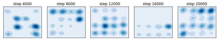
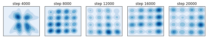
(a) Vanilla versus optimistic RMS (top and bottom respectively; $\gamma=3\times 10^{-4}$ in both cases).

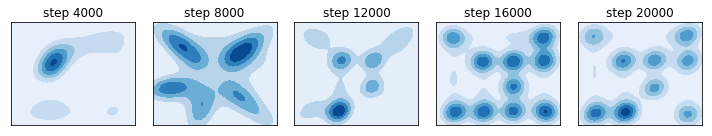
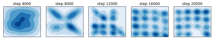
(b) Vanilla versus optimistic Adam (top and bottom respectively; $\gamma=4\times 10^{-5}$ in both cases).

Figure 2. Different algorithmic benchmarks (RMSprop and Adam): adding an extra-gradient step allows the training method to accurately learn the target data distribution and eliminates cycling and oscillatory instabilities.

For the experimental validation of our theoretical results, we began by evaluating the extra-gradient add-on in a highly multi-modal mixture of $16$ Gaussians arranged in a $4\times 4$ grid as in Metz et al. (2017). The generator and discriminator have $6$ fully connected layers with $384$ neurons and Relu activations (plus an additional layer for data space projection), and the generator generates $2$-dimensional vectors. The output after {4000, 8000, 12000, 16000, 20000} iterations is shown in Fig. 2. The networks were trained with RMSprop (Tieleman and Hinton, 2012) and Adam (Kingma and Ba, 2014), and the results are compared to the corresponding extra-gradient variant (for an explicit pseudocode representation in the case of Adam, see Daskalakis et al. (2018) and Appendix E). Learning rates and hyperparameters were chosen by an inspection of grid search results so as to enable a fair comparison between each method and its look-ahead version. Overall, the different optimization strategies without look-ahead exhibit mode collapse or oscillations throughout the training period (we ran all models for at least $20000$ iterations in order to evaluate the hopping behavior of the generator). In all cases, the extra-gradient add-on performs consistently better in learning the multi-modal distribution and greatly reduces occurrences of oscillatory behavior.

Experiments with standard datasets.

In our experiments with Gaussian mixture models, the most promising training method was Adam with an extra-gradient step (a concrete pseudocode implementation is provided in Appendix E). Motivated by this, we trained a Wasserstein-GAN on the CelebA and CIFAR-10 datasets using Adam, both with and without an extra-gradient step. The architecture employed was a standard DCGAN; hyperparameters and network architecture details may be found in Appendix E. Subsequently, to quantify the gains of the extra-gradient step, we employed the widely used inception score and Fréchet distance metrics, for which we report the results in Fig. 3. Under both metrics, the extra-gradient add-on provides consistently higher scores after an initial warm-up period (and is considerably more stable). For visualization purposes, we also present in Fig. 4 an ensemble of samples generated at the end of the training period. Overall, the generated samples provide accurate feature representation and low distortion (especially in CelebA).

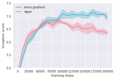
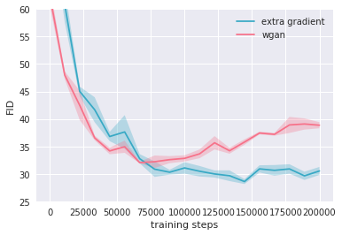
Figure 3. Left: Inception score (left) and Fréchet distance (right) on CIFAR-10 when training with Adam (with and without an extra-gradient step). Results are averaged over $8$ sample runs with different random seeds.

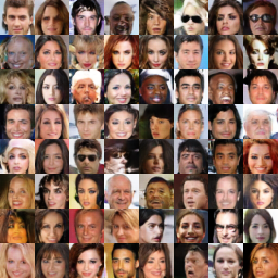
Figure 4. Samples generated by Adam with an extra-gradient step on CelebA (left) and CIFAR-10 (right).

6. Conclusions

Our results suggest that the implementation of an optimistic, extra-gradient step is a flexible add-on that can be easily attached to a wide variety of GAN training methods (RMSProp, Adam, SGA, etc.), and provides noticeable gains in performance and stability. From a theoretical standpoint, the dichotomy between strict and null coherence provides a justification of why this is so: optimism eliminates cycles and, in so doing, stabilizes the method. We find this property particularly appealing because it paves the way to a local analysis with provable convergence guarantees in multi-modal settings; we intend to examine this question in future work.

Appendix A Coherent saddle-point problems

We begin our discussion with some basic results on coherence:

Proposition A.1.

If $f$ is convex-concave, (SP) is coherent. In addition, if $f$ is strictly convex-concave, (SP) is strictly coherent.

Proof.

Let $x^{\ast}$ be a solution point of (SP). Since $f$ is convex-concave, first-order optimality gives

$$\langle g_{1}(x^{\ast}_{1},x^{\ast}_{2}),x_{1}-x^{\ast}_{1}\rangle =\langle\nabla_{x_{1}}f(x^{\ast}_{1},x^{\ast}_{2}),x_{1}-x^{\ast}_{1}\rangle\geq 0,$$ (A.1a)

and

$$\langle g_{2}(x^{\ast}_{1},x^{\ast}_{2}),x_{2}-x^{\ast}_{2}\rangle =\langle-\nabla_{x_{2}}f(x^{\ast}_{1},x^{\ast}_{2}),x_{2}-x^{\ast}_{2}\rangle\geq 0.$$ (A.1b)

Combining the two, we readily obtain the (Stampacchia) variational inequality

$$\langle g(x^{\ast}),x-x^{\ast}\rangle\geq 0\quad\text{for all $x\in\mathcal{X}$}.$$ (A.2)

In addition to the above, the fact that $f$ is convex-concave also implies that $g(x)$ is monotone in the sense that

$$\langle g(x^{\prime})-g(x),x^{\prime}-x\rangle\geq 0$$ (A.3)

for all $x,x^{\prime}\in\mathcal{X}$ Bauschke and Combettes (2017). Thus, setting $x^{\prime}\leftarrow x^{\ast}$ in (A.3) and invoking (A.2), we get

$$\langle g(x),x-x^{\ast}\rangle\geq\langle g(x^{\ast}),x-x^{\ast}\rangle\geq 0,$$ (A.4)

i.e., (VI) is satisfied.

To establish the converse implication, focus for concreteness on the minimizer, and note that (VI) implies that

$$\langle g_{1}(x),x_{1}-x^{\ast}_{1}\rangle\geq 0\quad\text{for all $x_{1}\in\mathcal{X}_{1}$}.$$ (A.5)

Now, if we fix some $x_{1}\in\mathcal{X}_{1}$ and consider the function $\phi(t)=f(x^{\ast}_{1}+t(x_{1}-x^{\ast}_{1}),x^{\ast}_{2})$, the inequality (A.5) yields

$$\phi^{\prime}(t) =\langle g(x^{\ast}_{1}+t(x_{1}-x^{\ast}_{1}),x^{\ast}_{2}),x_{1}-x^{\ast}_{1}\rangle$$

$$=\frac{1}{t}\langle g(x^{\ast}_{1}+t(x_{1}-x^{\ast}_{1}),x^{\ast}_{2}),x^{\ast}_{1}+t(x_{1}-x^{\ast}_{1}-x^{\ast}_{1}\rangle\geq 0,$$ (A.6)

for all $t\in[0,1]$. This implies that $\phi$ is nondecreasing, so $f(x_{1},x^{\ast}_{2})=\phi(1)\geq\phi(0)=f(x^{\ast}_{1},x^{\ast}_{2})$. The maximizing component follows similarly, showing that $x^{\ast}$ is a solution of (SP) and, in turn, establishing that (SP) is coherent.

For the strict part of the claim, the same line of reasoning shows that if $\langle g(x),x-x^{\ast}\rangle=0$ for some $x$ that is not a saddle-point of $f$, the function $\phi(t)$ defined above must be constant on $[0,1]$, indicating in turn that $f$ cannot be strictly convex-concave, a contradiction. ∎

We proceed to show that the solution set of a coherent saddle-point problem is closed (we will need this regularity result in the convergence analysis of Appendix C):

Lemma A.2.

Let $\mathcal{X}^{\ast}$ denote the solution set of (SP). If (SP) is coherent, $\mathcal{X}^{\ast}$ is closed.

Proof.

Let $x^{\ast}_{n}$, $n=1,2,\dotsc$, be a sequence of solutions of (SP) converging to some limit point $x^{\ast}\in\mathcal{X}$. To show that $\mathcal{X}^{\ast}$ is closed, it suffices to show that $x^{\ast}\in\mathcal{X}$.

Indeed, given that (SP) is coherent, every solution thereof satisfies (VI), so we have $\langle g(x),x-x^{\ast}_{n}\rangle\geq 0$ for all $x\in\mathcal{X}$. With $x^{\ast}_{n}\to x^{\ast}$ as $n\to\infty$, it follows that

$$\langle g(x),x-x^{\ast}\rangle=\lim_{n\to\infty}\langle g(x),x-x^{\ast}_{n}\rangle\geq 0\quad\text{for all $x\in\mathcal{X}$},$$ (A.7)

i.e., $x^{\ast}$ satisfies (VI). By coherence, this implies that $x^{\ast}$ is a solution of (SP), as claimed. ∎

Appendix B Properties of the Bregman divergence

In this appendix, we provide some auxiliary results and estimates that are used throughout the convergence analysis of Appendix C. Some of the results we present here (or close variants thereof) are not new (see e.g., Nemirovski et al., 2009; Juditsky et al., 2011). However, the hypotheses used to obtain them vary wildly in the literature, so we provide all the necessary details for completeness.

To begin, recall that the Bregman divergence associated to a $K$-strongly convex distance-generating function $h\colon\mathcal{X}\to\mathbb{R}$ is defined as

$$D(p,x)=h(p)-h(x)-\langle\nabla h(x),p-x\rangle$$ (B.1)

with $\nabla h(x)$ denoting a continuous selection of $\partial h(x)$. The induced prox-mapping is then given by

$$P_{x}(y) =\operatorname*{arg\,min}_{x^{\prime}\in\mathcal{X}}\{\langle y,x-x^{\prime}\rangle+D(x^{\prime},x)\}$$

$$=\operatorname*{arg\,max}_{x^{\prime}\in\mathcal{X}}\{\langle y+\nabla h(x),x^{\prime}\rangle-h(x^{\prime})\}$$ (B.2)

and is defined for all $x\in\operatorname{dom}\partial h$, $y\in\mathcal{Y}$ (recall here that $\mathcal{Y}\equiv\mathcal{V}^{\ast}$ denotes the dual of the ambient vector space $\mathcal{V}$). In what follows, we will also make frequent use of the convex conjugate $h^{\ast}\colon\mathcal{Y}\to\mathbb{R}$ of $h$, defined as

$$h^{\ast}(y)=\max_{x\in\mathcal{X}}\{\langle y,x\rangle-h(x)\}.$$ (B.3)

By standard results in convex analysis (Rockafellar, 1970, Chap. 26), $h^{\ast}$ is differentiable on $\mathcal{Y}$ and its gradient satisfies the identity

$$\nabla h^{\ast}(y)=\operatorname*{arg\,max}_{x\in\mathcal{X}}\{\langle y,x\rangle-h(x)\}.$$ (B.4)

For notational convenience, we will also write

$$Q(y)=\nabla h^{\ast}(y)$$ (B.5)

and we will refer to $Q\colon\mathcal{Y}\to\mathcal{X}$ as the mirror map generated by $h$. All these notions are related as follows:

Lemma B.1.

Let $h$ be a distance-generating function on $\mathcal{X}$. Then, for all $x\in\operatorname{dom}\partial h$, $y\in\mathcal{Y}$, we have:

$$a) \;\;x=Q(y) \;\iff\; y\in\partial h(x).$$ (B.6a)

$$b) \;\;x^{+}=P_{x}(y) \;\iff\; \nabla h(x)+y\in\partial h(x^{+}) \;\iff\; x^{+}=Q(\nabla h(x)+y).\hskip 40.00006pt$$ (B.6b)

Finally, if $x=Q(y)$ and $p\in\mathcal{X}$, we have

$$\langle\nabla h(x),x-p\rangle\leq\langle y,x-p\rangle.$$ (B.7)

Remark.

By (B.6b), we have $\partial h(x^{+})\neq\varnothing$, i.e., $x^{+}\in\operatorname{dom}\partial h$. As a result, the update rule $x\leftarrow P_{x}(y)$ is well-posed, i.e., it can be iterated in perpetuity.

Proof of Lemma B.1.

For (B.6a), note that $x$ solves (B.3) if and only if $y-\partial h(x)\ni 0$, i.e., if and only if $y\in\partial h(x)$. Similarly, comparing (B) with (B.3), it follows that $x^{+}$ solves (B) if and only if $\nabla h(x)+y\in\partial h(x^{+})$, i.e., if and only if $x^{+}=Q(\nabla h(x)+y)$.

For (B.7), by a simple continuity argument, it suffices to show that the inequality holds for interior $p\in\mathcal{X}^{\circ}$. To establish this, let

$$\phi(t)=h(x+t(p-x))-[h(x)+\langle y,x+t(p-x)\rangle].$$ (B.8)

Since $h$ is strongly convex and $y\in\partial h(x)$ by (B.6a), it follows that $\phi(t)\geq 0$ with equality if and only if $t=0$. Since $\psi(t)=\langle\nabla h(x+t(p-x))-y,p-x\rangle$ is a continuous selection of subgradients of $\phi$ and both $\phi$ and $\psi$ are continuous on $[0,1]$, it follows that $\phi$ is continuously differentiable with $\phi^{\prime}=\psi$ on $[0,1]$. Hence, with $\phi$ convex and $\phi(t)\geq 0=\phi(0)$ for all $t\in[0,1]$, we conclude that $\phi^{\prime}(0)=\langle\nabla h(x)-y,p-x\rangle\geq 0$, which proves our assertion. ∎

We continue with some basic bounds on the Bregman divergence before and after a prox step. The basic ingredient for these bounds is a generalization of the (Euclidean) law of cosines which is known in the literature as the “three-point identity” (Chen and Teboulle, 1993):

Lemma B.2.

Let $h$ be a distance-generating function on $\mathcal{X}$. Then, for all $p\in\mathcal{X}$ and all $x,x^{\prime}\in\operatorname{dom}\partial h$, we have

$$D(p,x^{\prime})=D(p,x)+D(x,x^{\prime})+\langle\nabla h(x^{\prime})-\nabla h(x),x-p\rangle.$$ (B.9)

Proof.

By definition, we have:

$$D(p,x^{\prime}) =h(p)-h(x^{\prime})-\langle\nabla h(x^{\prime}),p-x^{\prime}\rangle$$ (B.10)

$$D(p,x) =h(p)-h(x)-\langle\nabla h(x),p-x\rangle$$

$$D(x,x^{\prime}) =h(x)-h(x^{\prime})-\langle\nabla h(x^{\prime}),x-x^{\prime}\rangle.$$

Our claim then follows by adding the last two lines and subtracting the first. ∎

With this identity at hand, we have the following series of upper and lower bounds:

Proposition B.3.

Let $h$ be a $K$-strongly convex distance-generating function on $\mathcal{X}$, fix some $p\in\mathcal{X}$, and let $x^{+}=P_{x}(y)$ for $x\in\operatorname{dom}\partial h$, $y\in\mathcal{Y}$. We then have:

$$D(p,x)\hphantom{{}^{+}} \geq\frac{K}{2}\lVert x-p\rVert^{2}.$$ (B.11a)

$$D(p,x^{+}) \leq D(p,x)-D(x^{+},x)+\langle y,x^{+}-p\rangle$$ (B.11b)

$$\leq D(p,x)+\langle y,x-p\rangle+\frac{1}{2K}\lVert y\rVert_{\ast}^{2}$$ (B.11c)

Proof of (B.11a).

By the strong convexity of $h$, we get

$$h(p)\geq h(x)+\langle\nabla h(x),p-x\rangle+\frac{K}{2}\lVert p-x\rVert^{2}$$ (B.12)

so (B.11a) follows by gathering all terms involving $h$ and recalling the definition of $D(p,x)$. ∎

Proof of B.11b and B.11c.

By the three-point identity (B.9), we readily obtain

$$D(p,x)=D(p,x^{+})+D(x^{+},x)+\langle\nabla h(x)-\nabla h(x^{+}),x^{+}-p\rangle.$$ (B.13)

In turn, this gives

$$D(p,x^{+}) =D(p,x)-D(x^{+},x)+\langle\nabla h(x^{+})-\nabla h(x),x^{+}-p\rangle$$

$$\leq D(p,x)-D(x^{+},x)+\langle y,x^{+}-p\rangle,$$ (B.14)

where, in the last step, we used (B.7) and the fact that $x^{+}=P_{x}(y)$, so $\nabla h(x)+y\in\partial h(x^{+})$. The above is just (B.11b), so the first part of our proof is complete.

For (B.11c), the bound (B) gives

$$D(p,x^{+}) \leq D(p,x)+\langle y,x-p\rangle+\langle y,x^{+}-x\rangle-D(x^{+},x).$$ (B.15)

Therefore, by Young’s inequality (Rockafellar, 1970), we get

$$\langle y,x^{+}-x\rangle\leq\frac{K}{2}\lVert x^{+}-x\rVert^{2}+\frac{1}{2K}\lVert y\rVert_{\ast}^{2},$$ (B.16)

and hence

$$D(p,x^{+}) \leq D(p,x)+\langle y,x-p\rangle+\frac{1}{2K}\lVert y\rVert_{\ast}^{2}+\frac{K}{2}\lVert x^{+}-x\rVert^{2}-D(x^{+},x)$$

$$\leq D(p,x)+\langle y,x-p\rangle+\frac{1}{2K}\lVert y\rVert_{\ast}^{2},$$ (B.17)

with the last step following from Lemma B.1 applied to $x$ in place of $p$. ∎

The first part of Proposition B.3 shows that $X_{n}$ converges to $p$ if $D(p,X_{n})\to 0$. However, as we mentioned in the main body of the paper, the converse may fail: in particular, we could have $\liminf_{n\to\infty}D(p,X_{n})>0$ even if $X_{n}\to p$. To see this, let $\mathcal{X}$ be the $L^{2}$ ball of $\mathbb{R}^{d}$ and take $h(x)=-\sqrt{1-\lVert x\rVert_{2}^{2}}$. Then, a straightforward calculation gives

$$D(p,x)=\frac{1-\langle p,x\rangle}{\sqrt{1-\lVert x\rVert_{2}^{2}}}$$ (B.18)

whenever $\lVert p\rVert_{2}=1$. The corresponding level sets $L_{c}(p)=\{x\in\mathbb{R}^{d}:D(p,x)=c\}$ of $D(p,\cdot)$ are given by the equation

$$1-\langle p,x\rangle=c\sqrt{1-\lVert x\rVert_{2}^{2}},$$ (B.19)

which admits $p$ as a solution for all $c\geq 0$ (so $p$ belongs to the closure of $L_{c}(p)$ even though $D(p,p)=0$ by definition). As a result, under this distance-generating function, it is possible to have $X_{n}\to p$ even when $\liminf_{n\to\infty}D(p,X_{n})>0$ (simply take a sequence $X_{n}$ that converges to $p$ while remaining on the same level set of $D$). As we discussed in the main body of the paper, such pathologies are discarded by the Bregman reciprocity condition

$$D(p,X_{n})\to 0\quad\text{whenever}\quad X_{n}\to p.$$ (B.20)

This condition comes into play at the very last part of the proofs of Theorems 3.1 and 4.1; other than that, we will not need it in the rest of our analysis.

Finally, for the analysis of the OMD algorithm, we will need to relate prox steps taken along different directions:

Proposition B.4.

Let $h$ be a $K$-strongly convex distance-generating function on $\mathcal{X}$ and fix some $p\in\mathcal{X}$, $x\in\operatorname{dom}\partial h$. Then:

1. For all $y_{1},y_{2}\in\mathcal{Y}$, we have:

   $$\lVert P_{x}(y_{2})-P_{x}(y_{1})\rVert\leq\frac{1}{K}\lVert y_{2}-y_{1}\rVert_{\ast},$$ (B.21)

   i.e., $P_{x}$ is $(1/K)$-Lipschitz.

2. In addition, letting $x^{+}_{1}=P_{x}(y_{1})$ and $x^{+}_{2}=P_{x}(y_{2})$, we have:

   $$D(p,x^{+}_{2}) \leq D(p,x)+\langle y_{2},x^{+}_{1}-p\rangle+[\langle y_{2},x^{+}_{2}-x^{+}_{1}\rangle-D(x^{+}_{2},x)]$$ (B.22a)

   $$\leq D(p,x)+\langle y_{2},x^{+}_{1}-p\rangle+\frac{1}{2K}\lVert y_{2}-y_{1}\rVert_{\ast}^{2}-\frac{K}{2}\lVert x^{+}_{1}-x\rVert^{2}.$$ (B.22b)

Proof.

We begin with the proof of the Lipschitz property of $P_{x}$. Indeed, for all $p\in\mathcal{X}$, (B.7) gives

$$\langle\nabla h(x^{+}_{1})-\nabla h(x)-y_{1},x^{+}_{1}-p\rangle \leq 0,$$ (B.23a)

and

$$\langle\nabla h(x^{+}_{2})-\nabla h(x)-y_{2},x^{+}_{2}-p\rangle \leq 0.$$ (B.23b)

Therefore, setting $p\leftarrow x^{+}_{2}$ in (B.23a), $p\leftarrow x^{+}_{1}$ in (B.23b) and rearranging, we obtain

$$\langle\nabla h(x^{+}_{2})-\nabla h(x^{+}_{1}),x^{+}_{2}-x^{+}_{1}\rangle\leq\langle y_{2}-y_{1},x^{+}_{2}-x^{+}_{1}\rangle.$$ (B.24)

By the strong convexity of $h$, we also have

$$K\lVert x^{+}_{2}-x^{+}_{1}\rVert^{2}\leq\langle\nabla h(x^{+}_{2})-\nabla h(x^{+}_{1}),x^{+}_{2}-x^{+}_{1}\rangle.$$ (B.25)

Hence, combining B.25 and B.24, we get

$$K\lVert x^{+}_{2}-x^{+}_{1}\rVert^{2}\leq\langle y_{2}-y_{1},x^{+}_{2}-x^{+}_{1}\rangle\leq\lVert y_{2}-y_{1}\rVert_{\ast}\lVert x^{+}_{2}-x^{+}_{1}\rVert,$$ (B.26)

and our assertion follows.

For the second part of our claim, the bound (B.11b) of Proposition B.3 applied to $x^{+}_{2}=P_{x}(y_{2})$ readily gives

$$D(p,x^{+}_{2}) \leq D(p,x)-D(x^{+}_{2},x)+\langle y_{2},x^{+}_{2}-p\rangle$$

$$=D(p,x)+\langle y_{2},x^{+}_{1}-p\rangle+[\langle y_{2},x^{+}_{2}-x^{+}_{1}\rangle-D(x^{+}_{2},x)]$$ (B.27)

thus proving (B.22a). To complete our proof, note that (B.11b) with $p\leftarrow x^{+}_{2}$ gives

$$D(x^{+}_{2},x^{+}_{1})\leq D(x^{+}_{2},x)+\langle y_{1},x^{+}_{1}-x^{+}_{2}\rangle-D(x^{+}_{1},x),$$ (B.28)

or, after rearranging,

$$D(x^{+}_{2},x)\geq D(x^{+}_{2},x^{+}_{1})+D(x^{+}_{1},x)+\langle y_{1},x^{+}_{2}-x^{+}_{1}\rangle.$$ (B.29)

We thus obtain

$$\langle y_{2},x^{+}_{2}-x^{+}_{1}\rangle-D(x^{+}_{2},x) \leq\langle y_{2}-y_{1},x^{+}_{2}-x^{+}_{1}\rangle-D(x^{+}_{2},x^{+}_{1})-D(x^{+}_{1},x)$$

$$\leq\frac{\lVert y_{2}-y_{1}\rVert_{\ast}^{2}}{2K}+\frac{K}{2}\lVert x^{+}_{2}-x^{+}_{1}\rVert^{2}-\frac{K}{2}\lVert x^{+}_{2}-x^{+}_{1}\rVert^{2}-\frac{K}{2}\lVert x^{+}_{1}-x\rVert^{2}$$

$$\leq\frac{1}{2K}\lVert y_{2}-y_{1}\rVert_{\ast}^{2}-\frac{K}{2}\lVert x^{+}_{1}-x\rVert^{2},$$ (B.30)

where we used Young’s inequality and (B.11a) in the second inequality. The bound (B.22b) then follows by substituting (B) in (B). ∎

Appendix C Convergence analysis of mirror descent

We begin by recalling the definition of the mirror descent algorithm. With notation as in the previous section, the algorithm is defined via the recursive scheme

$$X_{n+1}=P_{X_{n}}(-\gamma_{n}\hat{g}_{n}),$$ (MD)

where $\gamma_{n}$ is a variable step-size sequence and $\hat{g}_{n}$ is the calculated value of the gradient vector $g(X_{n})$ at the $n$-th stage of the algorithm. As we discussed in the main body of the paper, the gradient input sequence $\hat{g}_{n}$ of (MD) is assumed to satisfy the standard oracle assumptions

$$a)\;\textit{Unbiasedness:} \operatorname{\mathbb{E}}[\hat{g}_{n}\nonscript\,|\nonscript\,\mathopen{}\mathcal{F}_{n}]=g(X_{n}).$$

$$b)\;\textit{Finite mean square:} \operatorname{\mathbb{E}}[\lVert\hat{g}_{n}\rVert_{\ast}^{2}\nonscript\,|\nonscript\,\mathopen{}\mathcal{F}_{n}]\leq G^{2}\;\;\text{for some finite $G\geq 0$}.\hskip 30.00005pt$$

where $\mathcal{F}_{n}$ represents the history (natural filtration) of the generating sequence $X_{n}$ up to stage $n$ (inclusive).

With this preliminaries at hand, our convergence proof for (MD) under strict coherence will hinge on the following results:

Proposition C.1.

Suppose that (SP) is coherent and (MD) is run with a gradient oracle satisfying (3.6) and a variable step-size $\gamma_{n}$ such that $\sum_{n=1}^{\infty}\gamma_{n}^{2}<\infty$. If $x^{\ast}\in\mathcal{X}$ is a solution of (SP), the Bregman divergence $D(x^{\ast},X_{n})$ converges (a.s.) to a random variable $D(x^{\ast})$ with $\operatorname{\mathbb{E}}[D(x^{\ast})]<\infty$.

Proposition C.2.

Suppose that (SP) is strictly coherent and (MD) is run with a gradient oracle satisfying (3.6) and a step-size $\gamma_{n}$ such that $\sum_{n=1}^{\infty}\gamma_{n}=\infty$ and $\sum_{n=1}^{\infty}\gamma_{n}^{2}<\infty$. Then, with probability $1$, there exists a (possibly random) solution $x^{\ast}$ of (SP) such that $\liminf_{n\to\infty}D(x^{\ast},X_{n})=0$.

Proposition C.1 can be seen as a “dichotomy” result: it shows that the Bregman divergence is an asymptotic constant of motion, so (MD) either converges to a saddle-point $x^{\ast}$ (if $D(x^{\ast})=0$) or to some nonzero level set of the Bregman divergence (with respect to $x^{\ast}$). In this way, Proposition C.1 rules out more complicated chaotic or aperiodic behaviors that may arise in general – for instance, as in the analysis of Palaiopanos et al. (2017) for the long-run behavior of the multiplicative weights algorithm in two-player games. However, unless this limit value can be somehow predicted (or estimated) in advance, this result cannot be easily applied. This is the main role of Proposition C.2: it shows that (MD) admits a subsequence converging to a solution of (SP) so, by (B.20), the limit of $D(x^{\ast},X_{n})$ must be zero.

With all this at hand, our first step is to prove Proposition C.1:

Proof of Proposition C.1.

Let $D_{n}=D(x^{\ast},X_{n})$ for some solution $x^{\ast}$ of (SP). Then, by Proposition B.3, we have

$$D_{n+1}=D(x^{\ast},P_{X_{n}}(-\gamma_{n}\hat{g}_{n})) \leq D(x^{\ast},X_{n})-\gamma_{n}\langle\hat{g}_{n},X_{n}-x^{\ast}\rangle+\frac{\gamma_{n}^{2}}{2K}\lVert\hat{g}_{n}\rVert^{2}$$

$$=D_{n}-\gamma_{n}\langle g(X_{n}),X_{n}-x^{\ast}\rangle-\gamma_{n}\langle U_{n+1},X_{n}-x^{\ast}\rangle+\frac{\gamma_{n}^{2}}{2K}\lVert\hat{g}_{n}\rVert_{\ast}^{2}$$

$$\leq D_{n}+\gamma_{n}\xi_{n+1}+\frac{\gamma_{n}^{2}}{2K}\lVert\hat{g}_{n}\rVert_{\ast}^{2},$$ (C.1)

where, in the last line, we set $\xi_{n+1}=-\langle U_{n+1},X_{n}-x^{\ast}\rangle$ and we invoked the assumption that (SP) is coherent. Thus, conditioning on $\mathcal{F}_{n}$ and taking expectations, we get

$$\operatorname{\mathbb{E}}[D_{n+1}\nonscript\,|\nonscript\,\mathopen{}\mathcal{F}_{n}]\leq D_{n}+\operatorname{\mathbb{E}}[\xi_{n+1}\nonscript\,|\nonscript\,\mathopen{}\mathcal{F}_{n}]+\frac{\gamma_{n}^{2}}{2K}\operatorname{\mathbb{E}}[\lVert\hat{g}_{n}\rVert_{\ast}^{2}\nonscript\,|\nonscript\,\mathopen{}\mathcal{F}_{n}]\leq D_{n}+\frac{G^{2}}{2K}\gamma_{n}^{2},$$ (C.2)

where we used the oracle assumptions (3.6) and the fact that $X_{n}$ is $\mathcal{F}_{n}$-measurable (by definition).

Now, letting $R_{n}=D_{n}+(2K)^{-1}G^{2}\sum_{k=n}^{\infty}\gamma_{k}^{2}$, the estimate (C) gives

$$\operatorname{\mathbb{E}}[R_{n+1}\nonscript\,|\nonscript\,\mathopen{}\mathcal{F}_{n}]=\operatorname{\mathbb{E}}[D_{n+1}\nonscript\,|\nonscript\,\mathopen{}\mathcal{F}_{n}]+\frac{G^{2}}{2K}\sum_{k=n+1}^{\infty}\gamma_{k}^{2}\leq D_{n}+\frac{G^{2}}{2K}\sum_{k=n}^{\infty}\gamma_{k}^{2}=R_{n},$$ (C.3)

i.e., $R_{n}$ is an $\mathcal{F}_{n}$-adapted supermartingale. Since $\sum_{n=1}^{\infty}\gamma_{n}^{2}<\infty$, it follows that

$$\operatorname{\mathbb{E}}[R_{n}]=\operatorname{\mathbb{E}}[\operatorname{\mathbb{E}}[R_{n}\nonscript\,|\nonscript\,\mathopen{}\mathcal{F}_{n-1}]]\leq\operatorname{\mathbb{E}}[R_{n-1}]\leq\dotsm\leq\operatorname{\mathbb{E}}[R_{1}]\leq\operatorname{\mathbb{E}}[D_{1}]+\frac{G^{2}}{2K}\sum_{n=1}^{\infty}\gamma_{n}^{2}<\infty,$$ (C.4)

i.e., $R_{n}$ is uniformly bounded in $L^{1}$. Thus, by Doob’s convergence theorem for supermartingales (Hall and Heyde, 1980, Theorem 2.5), it follows that $R_{n}$ converges (a.s.) to some finite random variable $R_{\infty}$ with $\operatorname{\mathbb{E}}[R_{\infty}]<\infty$. In turn, by inverting the definition of $R_{n}$, this shows that $D_{n}$ converges (a.s.) to some random variable $D(x^{\ast})$ with $\operatorname{\mathbb{E}}[D(x^{\ast})]<\infty$, as claimed. ∎

We now turn to the proof of existence of a convergent subsequence of (MD) under strict coherence (Proposition C.2):

Proof of Proposition C.2.

We begin with the technical observation that the solution set $\mathcal{X}^{\ast}$ of (SP) is closed – and hence, compact (cf. Lemma A.2 in Appendix A). Clearly, if $\mathcal{X}^{\ast}=\mathcal{X}$, there is nothing to show; hence, without loss of generality, we may assume in what follows that $\mathcal{X}^{\ast}\neq\mathcal{X}$.

Assume now ad absurdum that, with positive probability, the sequence $X_{n}$ generated by (MD) admits no limit points in $\mathcal{X}^{\ast}$. Conditioning on this event, and given that $\mathcal{X}^{\ast}$ is compact, there exists a (nonempty) compact set $\mathcal{C}\subset\mathcal{X}$ such that $\mathcal{C}\cap\mathcal{X}^{\ast}=\varnothing$ and $X_{n}\in\mathcal{C}$ for all sufficiently large $n$. Moreover, given that (SP) is strictly coherent, we have $\langle g(x),x-x^{\ast}\rangle>0$ whenever $x\in\mathcal{C}$ and $x^{\ast}\in\mathcal{X}^{\ast}$. Therefore, by the continuity of $g$ and the compactness of $\mathcal{X}^{\ast}$ and $\mathcal{C}$, there exists some $a>0$ such that

$$\langle g(x),x-x^{\ast}\rangle\geq a\quad\text{for all $x\in\mathcal{C}$, $x^{\ast}\in\mathcal{X}$}.$$ (C.5)

To proceed, fix some $x^{\ast}\in\mathcal{X}^{\ast}$ and let $D_{n}=D(x^{\ast},X_{n})$. Then, telescoping (C) yields the estimate

$$D_{n+1} \leq D_{1}-\sum_{k=1}^{n}\gamma_{k}\langle g(X_{k}),X_{k}-x^{\ast}\rangle+\sum_{k=1}^{n}\gamma_{k}\xi_{k+1}+\sum_{k=1}^{n}\frac{\gamma_{k}^{2}}{2K}\lVert\hat{g}_{k}\rVert_{\ast}^{2},$$ (C.6)

where, as in the proof of Proposition C.1, we set $\xi_{n+1}=\langle U_{n+1},X_{n}-x^{\ast}\rangle$. Subsequently, letting $\tau_{n}=\sum_{k=1}^{n}\gamma_{k}$ and using (C.5), we obtain

$$D_{n+1}\leq D_{1}-\tau_{n}\left[a-\frac{\sum_{k=1}^{n}\gamma_{k}\xi_{k+1}}{\tau_{n}}-\frac{(2K)^{-1}\sum_{k=1}^{n}\gamma_{k}^{2}\lVert\hat{g}_{k}\rVert_{\ast}^{2}}{\tau_{n}}\right].$$ (C.7)

By the unbiasedness hypothesis of (3.6) for $U_{n}$, we have $\operatorname{\mathbb{E}}[\xi_{n+1}\nonscript\,|\nonscript\,\mathopen{}\mathcal{F}_{n}]=\langle\operatorname{\mathbb{E}}[U_{n+1}\nonscript\,|\nonscript\,\mathopen{}\mathcal{F}_{n}],X_{n}-x^{\ast}\rangle=0$ (recall that $X_{n}$ is $\mathcal{F}_{n}$-measurable by construction). Moreover, since $U_{n}$ is bounded in $L^{2}$ and $\gamma_{n}$ is $\ell^{2}$ summable (by assumption), it follows that

$$\sum_{n=1}^{\infty}\gamma_{n}^{2}\operatorname{\mathbb{E}}[\xi_{n+1}^{2}\nonscript\,|\nonscript\,\mathopen{}\mathcal{F}_{n}] \leq\sum_{n=1}^{\infty}\gamma_{n}^{2}\lVert X_{n}-x^{\ast}\rVert^{2}\operatorname{\mathbb{E}}[\lVert U_{n+1}\rVert_{\ast}^{2}\nonscript\,|\nonscript\,\mathopen{}\mathcal{F}_{n}]$$

$$\leq\operatorname{diam}(\mathcal{X})^{2}\sigma^{2}\sum_{n=1}^{\infty}\gamma_{n}^{2}<\infty.$$ (C.8)

Therefore, by the law of large numbers for martingale difference sequences (Hall and Heyde, 1980, Theorem 2.18), we conclude that $\tau_{n}^{-1}\sum_{k=1}^{n}\gamma_{k}\xi_{k+1}$ converges to $0$ with probability $1$.

Finally, for the last term of (C.6), let $S_{n+1}=\sum_{k=1}^{n}\gamma_{k}^{2}\lVert\hat{g}_{k}\rVert_{\ast}^{2}$. Since $\hat{g}_{k}$ is $\mathcal{F}_{n}$-measurable for all $k=1,2,\dotsc,n-1$, we have

$$\operatorname{\mathbb{E}}[S_{n+1}\nonscript\,|\nonscript\,\mathopen{}\mathcal{F}_{n}]=\operatorname{\mathbb{E}}\left[\sum_{k=1}^{n-1}\gamma_{k}^{2}\lVert\hat{g}_{k}\rVert_{\ast}^{2}+\gamma_{n}^{2}\lVert\hat{g}_{n}\rVert_{\ast}^{2}\nonscript\,|\nonscript\,\mathopen{}\mathcal{F}_{n}\right]=S_{n}+\gamma_{n}^{2}\operatorname{\mathbb{E}}[\lVert\hat{g}_{n}\rVert_{\ast}^{2}\nonscript\,|\nonscript\,\mathopen{}\mathcal{F}_{n}]\geq S_{n},$$ (C.9)

i.e., $S_{n}$ is a submartingale with respect to $\mathcal{F}_{n}$. Furthermore, by the law of total expectation, we also have

$$\operatorname{\mathbb{E}}[S_{n+1}]=\operatorname{\mathbb{E}}[\operatorname{\mathbb{E}}[S_{n+1}\nonscript\,|\nonscript\,\mathopen{}\mathcal{F}_{n}]]\leq G^{2}\sum_{k=1}^{n}\gamma_{n}^{2}\leq G^{2}\sum_{k=1}^{\infty}\gamma_{n}^{2}<\infty,$$ (C.10)

so $S_{n}$ is bounded in $L^{1}$. Hence, by Doob’s submartingale convergence theorem (Hall and Heyde, 1980, Theorem 2.5), we conclude that $S_{n}$ converges to some (almost surely finite) random variable $S_{\infty}$ with $\operatorname{\mathbb{E}}[S_{\infty}]<\infty$, implying in turn that $\lim_{n\to\infty}S_{n+1}/\tau_{n}=0$ (a.s.).

Applying all of the above, the estimate (C.6) gives $D_{n+1}\leq D_{1}-a\tau_{n}/2$ for sufficiently large $n$, so $D(x^{\ast},X_{n})\to-\infty$, a contradiction. Going back to our original assumption, this shows that, with probability $1$, at least one of the limit points of $X_{n}$ must lie in $\mathcal{X}^{\ast}$, as claimed. ∎

With all this at hand, we are finally in a position to prove our main result for (MD):

Proof of Theorem 3.1(a).

Proposition C.2 shows that, with probability $1$, there exists a (possibly random) solution $x^{\ast}$ of (SP) such that $\liminf_{n\to\infty}\lVert X_{n}-x^{\ast}\rVert=0$ and, hence, $\liminf_{n\to\infty}D(x^{\ast},X_{n})=0$ (by Bregman reciprocity). Since $\lim_{n\to\infty}D(x^{\ast},X_{n})$ exists with probability $1$ (by Proposition C.1), it follows that $\lim_{n\to\infty}D(x^{\ast},X_{n})=\liminf_{n\to\infty}D(x^{\ast},X_{n})=0,$ i.e., $X_{n}$ converges to $x^{\ast}$. ∎

We proceed with the negative result hinted at in the main body of the paper, namely the failure of (MD) to converge under null coherence:

Proof of Theorem 3.1(b).

The evolution of the Bregman divergence under (MD) satisfies the identity

$$D(x^{\ast},X_{n+1}) =D(x^{\ast},X_{n})+D(X_{n},X_{n+1})+\gamma_{n}\langle\hat{g}_{n},X_{n}-x^{\ast}\rangle$$

$$=D(x^{\ast},X_{n})+D(X_{n},X_{n+1})+\langle U_{n+1},X_{n}-x^{\ast}\rangle$$ (C.11)

where, in the last line, we used the null coherence assumption $\langle g(x),x-x^{\ast}\rangle=0$ for all $x\in\mathcal{X}$. Since $D(X_{n},X_{n+1})\geq 0$, taking expecations above shows that $D(x^{\ast},X_{n})$ is nondecreasing, as claimed. ∎

With Theorem 3.1 at hand, the proof of Corollary 3.2 is an immediate consequence of the fact that strictly convex-concave problems satisfy strict coherence (Proposition A.1). As for Corollary 3.3, we provide below a more general result for two-player, zero-sum finite games.

To state it, let $\mathcal{A}_{i}=\{1,\dotsc,A_{i}\}$, $i=1,2$, be two finite sets of pure strategies, and let $\mathcal{X}_{i}=\operatorname{\Delta}(\mathcal{A}_{i})$ denote the set of mixed strategies of player $i$. A finite, two-player zero-sum game is then defined by a matrix $M\in\mathbb{R}^{\mathcal{A}_{1}\times\mathcal{A}_{2}}$ so that the loss of Player $1$ and the reward of Player $2$ in the mixed strategy profile $x=(x_{1},x_{2})\in\mathcal{X}$ are concurrently given by

$$f(x_{1},x_{2})=x_{1}^{\top}Mx_{2}$$ (C.12)

Then, writing $\Gamma\equiv\Gamma(\mathcal{A}_{1},\mathcal{A}_{2},M)$ for the resulting game, we have:

Proposition C.3.

Let $\Gamma$ be a two-player zero-sum game with an interior Nash equilibrium $x^{\ast}$. If $X_{1}\neq x^{\ast}$ and (MD) is run with exact gradient input ($\sigma^{2}=0$), we have $\lim_{n\to\infty}D(x^{\ast},X_{n})>0$. If, in addition, $\sum_{n=1}^{\infty}\gamma_{n}^{2}<\infty$, $\lim_{n\to\infty}D(x^{\ast},X_{n})$ is finite.

Remark.

Note that non-convergence does not require any summability assumptions on $\gamma_{n}$.

In words, Proposition C.3 states that (MD) does not converge in finite zero-sum games with a unique interior equilibrium and exact gradient input: instead, $X_{n}$ cycles at positive Bregman distance from the game’s Nash equilibrium. Heuristically, the reason for this behavior is that, for small $\gamma\to 0$, the incremental step $V_{\gamma}(x)=P_{x}(-\gamma g(x))-x$ of (MD) is essentially tangent to the level set of $D(x^{\ast},\cdot)$ that passes through $x$. For finite $\gamma>0$, things are even worse because $V_{\gamma}(x)$ points noticeably away from $x$, i.e., towards higher level sets of $D$. As a result, the “best-case scenario” for (MD) is to orbit $x^{\ast}$ (when $\gamma\to 0$); in practice, for finite $\gamma$, the algorithm takes small outward steps throughout its runtime, eventually converging to some limit cycle farther away from $x^{\ast}$.

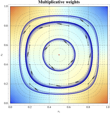
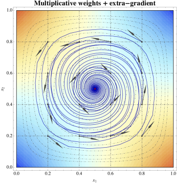
Figure 5. Trajectories of vanilla and optimistic mirror descent in a zero-sum game of Matching Pennies (left and right respectively). Colors represent the contours of the objective, $f(x_{1},x_{2})=(x_{1}-1/2)(x_{2}-1/2)$.

We make this intuition precise below (for a schematic illustration, see also Fig. 1 above):

Proof of Proposition C.3.

Write $v_{1}(x)=-Mx_{2}$ and $v_{2}(x)=x_{1}^{\top}M$ for the players’ payoff vectors under the mixed strategy profile $x=(x_{1},x_{2})$. By construction, we have $g(x)=-(v_{1}(x),v_{2}(x))$. Furthermore, since $x^{\ast}$ is an interior equilibrium of $f$, elementary game-theoretic considerations show that $v_{1}(x^{\ast})$ and $v_{2}(x^{\ast})$ are both proportional to the constant vector of ones. We thus get

$$\langle g(x),x-x^{\ast}\rangle =\langle v_{1}(x),x_{1}-x^{\ast}_{1}\rangle+\langle v_{2}(x),x_{2}-x^{\ast}_{2}\rangle$$

$$=-x_{1}^{\top}Mx_{2}+(x^{\ast}_{1})^{\top}Mx_{2}+x_{1}^{\top}Mx_{2}-x_{1}^{\top}Mx^{\ast}_{2}$$

$$=0,$$ (C.13)

where, in the last line, we used the fact that $x^{\ast}$ is interior. This shows that $f$ satisfies null coherence, so our claim follows from Theorem 3.1(b).

For our second claim, arguing as above and using (B.11c), we get

$$D(x^{\ast},X_{n+1}) \leq D(x^{\ast},X_{n})+\gamma_{n}\langle g(X_{n}),X_{n}-x^{\ast}\rangle+\frac{\gamma_{n}^{2}}{2K}\lVert g(X_{n})\rVert_{\ast}^{2}$$

$$\leq D(x^{\ast},X_{n})+\frac{\gamma_{n}^{2}G^{2}}{2K}$$ (C.14)

with $G=\max_{x_{1}\in\mathcal{X}_{1},x_{2}\in\mathcal{X}_{2}}\lVert(-Mx_{2},x_{1}^{\top}M)\rVert_{\ast}$. Telescoping this last bound yields

$$\sup_{n}D(x^{\ast},X_{n})\leq D(x^{\ast},X_{1})+\sum_{k=1}^{\infty}\frac{\gamma_{n}^{2}G^{2}}{2K}<\infty,$$ (C.15)

so $D(x^{\ast},X_{n})$ is also bounded from above. Therefore, with $D(x^{\ast},X_{n})$ nondecreasing, bounded from above and $D(x^{\ast},X_{1})>0$, it follows that $\lim_{n\to\infty}D(x^{\ast},X_{n})>0$, as claimed. ∎

Appendix D Convergence analysis of optimistic mirror descent

We now turn to the optimistic mirror descent (OMD) algorithm, as defined by the recursion

$$X_{n+1/2} =P_{X_{n}}(-\gamma_{n}\hat{g}_{n})$$ (OMD)

$$X_{n+1} =P_{X_{n}}(-\gamma_{n}\hat{g}_{n+1/2})$$

with $X_{1}$ initialized arbitrarily in $\operatorname{dom}\partial h$, and $\hat{g}_{n}$, $\hat{g}_{n+1/2}$ representing gradient oracle queries at the incumbent and intermediate states $X_{n}$ and $X_{n+1/2}$ respectively.

The heavy lifting for our analysis is provided by Proposition B.4, which leads to the following crucial lemma:

Lemma D.1.

Suppose that (SP) is coherent and $g$ is $L$-Lipschitz continuous. With notation as above and exact gradient input ($\sigma=0$), we have

$$D(x^{\ast},X_{n+1})\leq D(x^{\ast},X_{n})-\frac{1}{2}\left(K-\frac{\gamma_{n}^{2}L^{2}}{K}\right)\lVert X_{n+1/2}-X_{n}\rVert^{2},$$ (D.1)

for every solution $x^{\ast}$ of (SP).

Proof.

Substituting $x\leftarrow X_{n}$, $y_{1}\leftarrow-\gamma_{n}g(X_{n})$, and $y_{2}\leftarrow-\gamma_{n}g(X_{n+1/2})$ in Proposition B.4, we obtain the estimate:

$$D(x^{\ast},X_{n+1}) \leq D(x^{\ast},X_{n})-\gamma_{n}\langle g(X_{n+1/2}),X_{n+1/2}-x^{\ast}\rangle$$

$$+\frac{\gamma_{n}^{2}}{2K}\lVert g(X_{n+1/2})-g(X_{n})\rVert_{\ast}^{2}-\frac{K}{2}\lVert X_{n+1/2}-X_{n}\rVert^{2}$$

$$\leq D(x^{\ast},X_{n})+\frac{\gamma_{n}^{2}L^{2}}{2K}\lVert X_{n+1/2}-X_{n}\rVert^{2}-\frac{K}{2}\lVert X_{n+1/2}-X_{n}\rVert^{2},$$ (D.2)

where, in the last line, we used the fact that $x^{\ast}$ is a solution of (SP)/(VI), and that $g$ is $L$-Lipschitz. ∎

We are now finally in a position to prove Theorem 4.1 (reproduced below for convenience):

Theorem.

Suppose that (SP) is coherent and $g$ is $L$-Lipschitz continuous. If (OMD) is run with exact gradient input and a step-size sequence $\gamma_{n}$ such that

$$\textstyle 0<\lim_{n\to\infty}\gamma_{n}\leq\sup_{n}\gamma_{n}<K/L,$$ (D.3)

the sequence $X_{n}$ converges monotonically to a solution $x^{\ast}$ of (SP), i.e., $D(x^{\ast},X_{n})$ is non-increasing and converges to $0$.

Proof.

Let $x^{\ast}$ be a solution of (SP). Then, by the stated assumptions for $\gamma_{n}$, Lemma D.1 yields

$$D(x^{\ast},X_{n+1})\leq D(x^{\ast},X_{n})-\frac{1}{2}K(1-\alpha^{2})\lVert X_{n+1/2}-X_{n}\rVert^{2},$$ (D.4)

where $\alpha\in(0,1)$ is such that $\gamma_{n}^{2}<\alpha K/L$ for all $n$ (that such an $\alpha$ exists is a consequence of the assumption that $\sup_{n}\gamma_{n}<K/L$). This shows that $D(x^{\ast},X_{n})$ is non-decreasing for every solution $x^{\ast}$ of (SP).

Now, telescoping (D.1), we obtain

$$D(x^{\ast},X_{n+1})\leq D(x^{\ast},X_{1})-\frac{1}{2}\sum_{k=1}^{n}\left(K-\frac{\gamma_{k}^{2}L^{2}}{K}\right)\lVert X_{k+1/2}-X_{k}\rVert^{2},$$ (D.5)

and hence:

$$\sum_{k=1}^{n}\left(1-\frac{\gamma_{k}^{2}L^{2}}{K^{2}}\right)\lVert X_{k+1/2}-X_{k}\rVert^{2}\leq\frac{2}{K}D(x^{\ast},X_{1}).$$ (D.6)

With $\sup_{n}\gamma_{n}<K/L$, the above estimate readily yields $\sum_{n=1}^{\infty}\lVert X_{n+1/2}-X_{n}\rVert^{2}<\infty$, which in turn implies that $\lVert X_{n+1/2}-X_{n}\rVert\to 0$ as $n\to\infty$.

By the compactness of $\mathcal{X}$, we further infer that $X_{n}$ admits an accumulation point $\hat{x}$, i.e., there exists a subsequence $n_{k}$ such that $X_{n_{k}}\to\hat{x}$ as $k\to\infty$. Since $\lVert X_{n_{k}+1/2}-X_{n_{k}}\rVert\to 0$, this also implies that $X_{n_{k}+1/2}$ converges to $\hat{x}$ as $k\to\infty$. Further, by passing to a subsequence if necessary, we may also assume without loss of generality that $\gamma_{n_{k}}$ converges to some limit value $\gamma>0$. Then, by the Lipschitz continuity of the prox-mapping (cf. Proposition B.4), we readily obtain

$$\hat{x}=\lim_{k\to\infty}X_{n_{k}+1/2}=\lim_{k\to\infty}P_{X_{n_{k}}}(X_{n_{k}}-\gamma_{n_{k}}g(X_{n_{k}}))=P_{\hat{x}}(\hat{x}-\gamma g(\hat{x})),$$ (D.7)

i.e., $\hat{x}$ is a solution of (VI) – and, hence, (SP). Since $D(\hat{x},X_{n})$ is nonincreasing and $\liminf_{n\to\infty}D(\hat{x},X_{n})=0$ (by the Bregman reciprocity requirement), we conclude that $\liminf_{n\to\infty}D(\hat{x},X_{n})=0$, i.e., $X_{n}$ converges to $\hat{x}$. Since $\hat{x}$ is a solution of (SP), our proof is complete. ∎

Our last result concerns the convergence of (OMD) in strictly coherent problems with a stochastic gradient oracle:

Proof of Theorem 4.3.

Our argument hinges on the inequality

$$D(x^{\ast},X_{n+1})\leq D(x^{\ast},X_{n})-\gamma_{n}\langle\hat{g}_{n+1/2},X_{n+1/2}-x^{\ast}\rangle+\gamma_{n}^{2}/(2K)\,\lVert\hat{g}_{n+1/2}-\hat{g}_{n}\rVert_{\ast}^{2}$$ (D.8)

which is obtained from the two-point estimate (B.22b) by substituting $x\leftarrow x^{\ast}$, $x_{1}\leftarrow X_{n}$, $y_{1}\leftarrow\hat{g}_{n}$, $x^{+}_{1}\leftarrow X_{n+1/2}=P_{X_{n}}(-\gamma_{n}\hat{g}_{n})$, $y_{2}\leftarrow\hat{g}_{n+1/2}$, and $x^{+}_{2}\leftarrow X_{n}=P_{X_{n}}(-\gamma_{n}\hat{g}_{n+1/2})$. Then, working as in the proof of Proposition C.1, we obtain the following estimate for the sequence $D_{n}=D(x^{\ast},X_{n})$:

$$D_{n+1} \leq D_{n}-\gamma_{n}\langle g(X_{n+1/2}),X_{n+1/2}-x^{\ast}\rangle-\gamma_{n}\langle U^{+}_{n+1},X_{n}-x^{\ast}\rangle+\frac{\gamma_{n}^{2}}{2K}\lVert\hat{g}_{n+1/2}-\hat{g}_{n}\rVert_{\ast}^{2}$$

$$\leq D_{n}+\gamma_{n}\xi^{+}_{n+1}+\frac{\gamma_{n}^{2}}{K}\left[\lVert\hat{g}_{n}\rVert_{\ast}^{2}+\lVert\hat{g}_{n+1/2}^{2}\rVert_{\ast}\right],$$ (D.9)

where $U^{+}_{n+1}=\hat{g}_{n+1/2}-g(X_{n+1/2})$ denotes the martingale part of $\hat{g}_{n+1/2}$ and we have set $\xi^{+}_{n+1}=\langle U^{+}_{n+1},X_{n+1/2}-x^{\ast}\rangle$. Since $\operatorname{\mathbb{E}}[\lVert g_{n}\rVert_{\ast}^{2}\nonscript\,|\nonscript\,\mathopen{}X_{n},\dotsc,X_{1}]$ and $\operatorname{\mathbb{E}}[\lVert g_{n+1/2}\rVert_{\ast}^{2}\nonscript\,|\nonscript\,\mathopen{}X_{n+1/2},\dotsc,X_{1}]$ are both bounded by $G^{2}$, we get the bound

$$\operatorname{\mathbb{E}}[D_{n+1}\nonscript\,|\nonscript\,\mathopen{}\mathcal{F}_{n}]\leq D_{n}+\frac{G}{K}\gamma_{n}^{2}.$$ (D.10)

Then, following the same steps as in the proof of Proposition C.1, it follows that $D_{n}$ converges to some limit value $D_{\infty}$.

To proceed, telescoping (D) also yields

$$D_{n+1}\leq D_{1}-\sum_{k=1}^{n}\gamma_{k}\langle g(X_{k+1/2}),X_{k+1/2}-x^{\ast}\rangle+\sum_{k=1}^{n}\gamma_{k}\xi^{+}_{k+1}+\sum_{k=1}^{n}\frac{\gamma_{k}^{2}}{2K}\lVert\hat{g}_{k+1/2}-\hat{g}_{k}\rVert_{\ast}^{2}.$$ (D.11)

Each term in the above bound can be controlled in the same way as the corresponding terms in (C.6). Thus, repeating the steps in the proof of Proposition C.2, it follows that there exists a subsequence of $X_{n+1/2}$ (and hence also of $X_{n}$) which converges to $x^{\ast}$.

Our claim then follows by combining the two intermediate results above in the same way as in the proof of Theorem 3.1(a); to avoid needless repetition, we omit the details. ∎

Appendix E Experimental results

E.1. Adam with extra-gradient step

For most of our experiments, the method that seemed to generate the best results was Adam and its optimistic version (Daskalakis et al., 2018); for a pseudocode iplementation, see LABEL:alg:extra_Adam below. We also noticed empirically that it was more efficient to use two different sets of moment estimates $(m_{t},v_{t})$ and $(m_{t}^{\prime},v_{t}^{\prime})$ for the first and the second gradient steps. We used this algorithm for our experiments with both GMMs and the CelebA/CIFAR-10 datasets.

E.2. Experiments with standards datasets

In this section we present the results of our image experiments using OMD training techniques. Inception and FID scores obtained by our model during training were reported in Fig. 3: as can be seen there, the extra-gradient add-on improves the performance of GAN training and efficiently stabilizes the model; without the extra-gradient step, performance tends to drop noticeably after approximately $100k$ steps.

For ease of comparison, we provide below a collection of samples generated by Adam and optimistic Adam in the CelebA and CIFAR-10 datasets. Especially in the case of CelebA, the generated samples are consistently more representative and faithful to the target data distribution.

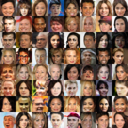
(a) Vanilla versus optimistic Adam training in the CelebA dataset (left and right respectively).

(b) Vanilla versus optimistic Adam training in the CIFAR-10 dataset (left and right respectively).

Figure 6. GAN training with and without an extra-gradient step in the CelebA and CIFAR-10 datasets.

E.2.1. Network Architecture and hyperparameters

For the reproducibility of our experiments, we provide Table 1 and Table 2 the network architectures and the hyperparameters of the GANs that we used. The architecture employed is a standard DCGAN architecture with a $5$-layer generator with batchnorm, and an $8$-layer discriminator. The generated samples were 32$\times$32$\times$3 RGB images.

Table 1. Generator and discriminator architectures for our images experiments

Generator
latent space 100 (gaussian noise)
dense 4 $\times$ 4 $\times$ 512 batchnorm ReLU
4$\times$4 conv.T stride=2 256 batchnorm ReLU
4$\times$4 conv.T stride=2 128 batchnorm ReLU
4$\times$4 conv.T stride=2 64 batchnorm ReLU
4$\times$4 conv.T stride=1 3 weightnorm tanh
Discriminator
Input Image 32$\times$32$\times$3
3$\times$3 conv. stride=1 64 lReLU
3$\times$3 conv. stride=2 128 lReLU
3$\times$3 conv. stride=1 128 lReLU
3$\times$3 conv. stride=2 256 lReLU
3$\times$3 conv. stride=1 256 lReLU
3$\times$3 conv. stride=2 512 lReLU
3$\times$3 conv. stride=1 512 lReLU
dense 1

Table 2. Image experiments settings

batch size = 64 Adam learning rate = 0.0001

Adam $\beta_{1}=0.0$

Adam $\beta_{2}=0.9$

max iterations = 200000

WGAN-GP $\lambda=1.0$

WGAN-GP $n_{dis}=1$

GAN objective = ’WGAN-GP’

Optimizer = ’extra-Adam’ or ’Adam’

References

• Arjovsky et al. (2017) Arjovsky, Martín, Soumith Chintala, Léon Bottou. 2017. Wasserstein generative adversarial networks. Proceedings of the 34th International Conference on Machine Learning, ICML 2017, Sydney, NSW, Australia, 6-11 August 2017. 214–223. URL http://proceedings.mlr.press/v70/arjovsky17a.html.
• Arora et al. (2012) Arora, Sanjeev, Elad Hazan, Satyen Kale. 2012. The multiplicative weights update method: A meta-algorithm and applications. Theory of Computing 8(1) 121–164.
• Auer et al. (1995) Auer, Peter, Nicolò Cesa-Bianchi, Yoav Freund, Robert E. Schapire. 1995. Gambling in a rigged casino: The adversarial multi-armed bandit problem. Proceedings of the 36th Annual Symposium on Foundations of Computer Science.
• Bailey and Piliouras (2018) Bailey, James P, Georgios Piliouras. 2018. Multiplicative weights update in zero-sum games. Proceedings of the 2018 ACM Conference on Economics and Computation. ACM, 321–338.
• Bauschke and Combettes (2017) Bauschke, Heinz H., Patrick L. Combettes. 2017. Convex Analysis and Monotone Operator Theory in Hilbert Spaces. 2nd ed. Springer, New York, NY, USA.
• Bhojanapalli et al. (2016) Bhojanapalli, Srinadh, Behnam Neyshabur, Nati Srebro. 2016. Global optimality of local search for low rank matrix recovery. Advances in Neural Information Processing Systems. 3873–3881.
• Bottou (1998) Bottou, Léon. 1998. Online learning and stochastic approximations. On-line learning in neural networks 17(9) 142.
• Bregman (1967) Bregman, Lev M. 1967. The relaxation method of finding the common point of convex sets and its application to the solution of problems in convex programming. USSR Computational Mathematics and Mathematical Physics 7(3) 200–217.
• Bubeck (2015) Bubeck, Sébastien. 2015. Convex optimization: Algorithms and complexity. Foundations and Trends in Machine Learning 8(3-4) 231–358.
• Chen and Teboulle (1993) Chen, Gong, Marc Teboulle. 1993. Convergence analysis of a proximal-like minimization algorithm using Bregman functions. SIAM Journal on Optimization 3(3) 538–543.
• Daskalakis et al. (2018) Daskalakis, Constantinos, Andrew Ilyas, Vasilis Syrgkanis, Haoyang Zeng. 2018. Training GANs with optimism. ICLR ’18: Proceedings of the 2018 International Conference on Learning Representations.
• Facchinei and Pang (2003) Facchinei, Francisco, Jong-Shi Pang. 2003. Finite-Dimensional Variational Inequalities and Complementarity Problems. Springer Series in Operations Research, Springer.
• Freund and Schapire (1999) Freund, Yoav, Robert E. Schapire. 1999. Adaptive game playing using multiplicative weights. Games and Economic Behavior 29 79–103.
• Ge et al. (2015) Ge, Rong, Furong Huang, Chi Jin, Yang Yuan. 2015. Escaping from saddle points online stochastic gradient for tensor decomposition. Conference on Learning Theory. 797–842.
• Ge et al. (2017) Ge, Rong, Chi Jin, Yi Zheng. 2017. No spurious local minima in nonconvex low rank problems: A unified geometric analysis. arXiv preprint arXiv:1704.00708 .
• Ge et al. (2016) Ge, Rong, Jason D Lee, Tengyu Ma. 2016. Matrix completion has no spurious local minimum. Advances in Neural Information Processing Systems. 2973–2981.
• Gidel et al. (2018) Gidel, Gauthier, Hugo Berard, Pascal Vincent, Simon Lacoste-Julien. 2018. A variational inequality perspective on generative adversarial networks. https://arxiv.org/pdf/1802.10551.pdf.
• Goodfellow et al. (2014) Goodfellow, Ian, Jean Pouget-Abadie, Mehdi Mirza, Bing Xu, David Warde-Farley, Sherjil Ozair, Aaron Courville, Yoshua Bengio. 2014. Generative adversarial nets. Advances in neural information processing systems. 2672–2680.
• Gulrajani et al. (2017) Gulrajani, Ishaan, Faruk Ahmed, Martin Arjovsky, Vincent Dumoulin, Aaron Courville. 2017. Improved training of wasserstein gans. Advances in Neural Information Processing Systems 30 (NIPS 2017). Curran Associates, Inc., 5769–5779. URL https://papers.nips.cc/paper/7159-improved-training-of-wasserstein-gans. Arxiv: 1704.00028.
• Hall and Heyde (1980) Hall, P., C. C. Heyde. 1980. Martingale Limit Theory and Its Application. Probability and Mathematical Statistics, Academic Press, New York.
• Hazan (2012) Hazan, Elad. 2012. A survey: The convex optimization approach to regret minimization. Suvrit Sra, Sebastian Nowozin, Stephen J. Wright, eds., Optimization for Machine Learning. MIT Press, 287–304.
• Juditsky et al. (2011) Juditsky, Anatoli, Arkadi Semen Nemirovski, Claire Tauvel. 2011. Solving variational inequalities with stochastic mirror-prox algorithm. Stochastic Systems 1(1) 17–58.
• Kingma and Ba (2014) Kingma, Diederik, Jimmy Ba. 2014. Adam: A method for stochastic optimization .
• Kiwiel (1997) Kiwiel, Krzysztof C. 1997. Free-steering relaxation methods for problems with strictly convex costs and linear constraints. Mathematics of Operations Research 22(2) 326–349.
• Korpelevich (1976) Korpelevich, G. M. 1976. The extragradient method for finding saddle points and other problems. Èkonom. i Mat. Metody 12 747–756.
• Lee et al. (2017) Lee, Jason D, Ioannis Panageas, Georgios Piliouras, Max Simchowitz, Michael I Jordan, Benjamin Recht. 2017. First-order methods almost always avoid saddle points. arXiv preprint arXiv:1710.07406 .
• Lee et al. (2016) Lee, Jason D, Max Simchowitz, Michael I Jordan, Benjamin Recht. 2016. Gradient descent only converges to minimizers. Conference on Learning Theory. 1246–1257.
• Mertikopoulos et al. (2018) Mertikopoulos, Panayotis, Christos H. Papadimitriou, Georgios Piliouras. 2018. Cycles in adversarial regularized learning. SODA ’18: Proceedings of the 29th annual ACM-SIAM Symposium on Discrete Algorithms.
• Mescheder et al. (2018) Mescheder, Lars, Andreas Geiger, Sebastian Nowozin. 2018. Which training methods for GANs do actually converge? https://arxiv.org/abs/1801.04406.
• Metz et al. (2017) Metz, Luke, Ben Poole, David Pfau, Jascha Sohl-Dickstein. 2017. Unrolled generative adversarial networks. ICLR Proceedings .
• Nemirovski (2004) Nemirovski, Arkadi Semen. 2004. Prox-method with rate of convergence ${O}(1/t)$ for variational inequalities with Lipschitz continuous monotone operators and smooth convex-concave saddle point problems. SIAM Journal on Optimization 15(1) 229–251.
• Nemirovski et al. (2009) Nemirovski, Arkadi Semen, Anatoli Juditsky, Guanghui Lan, Alexander Shapiro. 2009. Robust stochastic approximation approach to stochastic programming. SIAM Journal on Optimization 19(4) 1574–1609.
• Nemirovski and Yudin (1983) Nemirovski, Arkadi Semen, David Berkovich Yudin. 1983. Problem Complexity and Method Efficiency in Optimization. Wiley, New York, NY.
• Nesterov (2007) Nesterov, Yurii. 2007. Dual extrapolation and its applications to solving variational inequalities and related problems. Mathematical Programming 109(2) 319–344.
• Palaiopanos et al. (2017) Palaiopanos, Gerasimos, Ioannis Panageas, Georgios Piliouras. 2017. Multiplicative weights update with constant step-size in congestion games: Convergence, limit cycles and chaos. NIPS ’17: Proceedings of the 31st International Conference on Neural Information Processing Systems.
• Panageas and Piliouras (2017) Panageas, Ioannis, Georgios Piliouras. 2017. Gradient descent only converges to minimizers: Non-isolated critical points and invariant regions. Innovations of Theoretical Computer Science (ITCS).
• Papadimitriou and Piliouras (2016) Papadimitriou, Christos, Georgios Piliouras. 2016. From nash equilibria to chain recurrent sets: Solution concepts and topology. ITCS.
• Piliouras and Shamma (2014) Piliouras, Georgios, Jeff S Shamma. 2014. Optimization despite chaos: Convex relaxations to complex limit sets via poincaré recurrence. Proceedings of the twenty-fifth annual ACM-SIAM symposium on Discrete algorithms. SIAM, 861–873.
• Radford et al. (2015) Radford, A., L. Metz, S. Chintala. 2015. Unsupervised Representation Learning with Deep Convolutional Generative Adversarial Networks. ArXiv e-prints .
• Rakhlin and Sridharan (2013) Rakhlin, Alexander, Karthik Sridharan. 2013. Optimization, learning, and games with predictable sequences. NIPS ’13: Proceedings of the 26th International Conference on Neural Information Processing Systems.
• Rockafellar (1970) Rockafellar, Ralph Tyrrell. 1970. Convex Analysis. Princeton University Press, Princeton, NJ.
• Salimans et al. (2016) Salimans, Tim, Ian J. Goodfellow, Wojciech Zaremba, Vicki Cheung, Alec Radford, Xi Chen. 2016. Improved techniques for training gans. NIPS. 2234–2242.
• Shalev-Shwartz (2011) Shalev-Shwartz, Shai. 2011. Online learning and online convex optimization. Foundations and Trends in Machine Learning 4(2) 107–194.
• Sun et al. (2016) Sun, Ju, Qing Qu, John Wright. 2016. A geometric analysis of phase retrieval. Information Theory (ISIT), 2016 IEEE International Symposium on. IEEE, 2379–2383.
• Sun et al. (2017a) Sun, Ju, Qing Qu, John Wright. 2017a. Complete dictionary recovery over the sphere i: Overview and the geometric picture. IEEE Transactions on Information Theory 63(2) 853–884.
• Sun et al. (2017b) Sun, Ju, Qing Qu, John Wright. 2017b. Complete dictionary recovery over the sphere ii: Recovery by riemannian trust-region method. IEEE Transactions on Information Theory 63(2) 885–914.
• Tieleman and Hinton (2012) Tieleman, T., G. Hinton. 2012. Lecture 6.5 - rmsprop, coursera: Neural networks for machine learning .
• Zhou et al. (2017) Zhou, Zhengyuan, Panayotis Mertikopoulos, Nicholas Bambos, Stephen Boyd, Peter W. Glynn. 2017. Stochastic mirror descent for variationally coherent optimization problems. NIPS ’17: Proceedings of the 31st International Conference on Neural Information Processing Systems.