Numerical computation of endomorphism rings of Jacobians

Abstract.

We give practical numerical methods to compute the period matrix of a plane algebraic curve (not necessarily smooth). We show how automorphisms and isomorphisms of such curves, as well as the decomposition of their Jacobians up to isogeny, can be calculated heuristically. Particular applications include the determination of (generically) non-Galois morphisms between curves and the identification of Prym varieties.

1. Introduction

Let $k$ be a field of characteristic $0$ that is finitely generated over $\mathbb{Q}$. We choose an embedding of $k$ into $\mathbb{C}$. In this article, we consider nonsingular, complete, absolutely irreducible algebraic curves $C$ over $k$ of genus $g$. We represent such a curve $C$ by a possibly singular affine plane model

(1.1) $$\widetilde{C}\colon f(x,y)=0,\text{ where }f(x,y)\in k[x,y].$$

Associated to $C$ is the Jacobian variety $J=\operatorname{Jac}(C)$ representing $\operatorname{Pic}^{0}(C)$. Classical results by Abel and Jacobi establish

$$J(\mathbb{C})\cong\operatorname{H}^{0}(C_{\mathbb{C}},\Omega_{C}^{1})^{*}/\operatorname{H}_{1}(C(\mathbb{C}),\mathbb{Z})\cong\mathbb{C}^{g}/\Omega\mathbb{Z}^{2g},$$

for a suitable $g\times 2g$ matrix $\Omega$, called a period matrix of $C$.

Let $J_{1}=\operatorname{Jac}(C_{1})$ and $J_{2}=\operatorname{Jac}(C_{2})$ be two such Jacobian varieties. The $\mathbb{Z}$-module $\operatorname{Hom}_{\overline{k}}(J_{1},J_{2})$ of homomorphisms defined over the algebraic closure $\overline{k}$ of $k$ is finitely generated and can be represented as the group of $\mathbb{C}$-linear maps $\mathbb{C}^{g_{1}}\to\mathbb{C}^{g_{2}}$ mapping the columns of $\Omega_{1}$ into $\Omega_{2}\mathbb{Z}^{g_{2}}$. As described in [CMSV, §2.2], we can heuristically determine homomorphism modules, along with their tangent representations, from numerical approximations to $\Omega_{1},\Omega_{2}$. These can then serve as input for rigorous verification as in loc. cit.

In this article we consider the problem of computing approximations to period matrices for arbitrary algebraic curves for the purpose of numerically determining homomorphism modules and endomorphism rings. We also describe how to identify the (finite) symplectic automorphism groups in these rings, and with that the automorphism group of the curve. We give several examples of how the heuristic determination of such objects can be used to obtain rigorous results.

There is extensive earlier work on computing period matrices for applications in scientific computing to Riemann theta functions and partial differential equations. For these applications, approximations that fit in standard machine precision tend to be sufficient. Number-theoretic applications tend to need higher accuracy and use arbitrary-precision approximation. Hyperelliptic curves have received most attention, see for instance Van Wamelen’s [vanWamelen2006] implementation in Magma. In practice it is limited to about 2000 digits. Recent work by Molin–Neurohr [molin-neurohr] can reach higher accuracy and also applies to superelliptic curves.

For general curves, a Maple package based on Deconinck and Van Hoeij [DeconinckVanHoeij2001] computes period matrices at system precision or (much more slowly) at arbitrary precision. Swierczewski’s reimplementation in SageMath [swier] only uses machine precision and no high-order numerical integration. During the writing of this article, another new and fast Magma implementation was developed by Neurohr [neurohr-thesis]. See the introduction of [neurohr-thesis] for a more comprehensive overview of the history and recent work on the subject.

Our approach is similar to the references above (in contrast to, for instance, the deformation approach taken in [sertoz2018]) in that we basically use the definition of the period matrix to compute an approximation.

Algorithm Compute approximation to period matrix.

Input: $f$ as in (1.1) over a number field and a given working precision.

Output: Approximation of a period matrix of the described curve.

1. Determine generators of the fundamental group of $C$ (Section 2.3).

2. Derive a symplectic basis $\left\{\alpha_{1},\ldots\alpha_{g},\beta_{1},\ldots,\beta_{g}\right\}$ of the homology group $H_{1}(C(\mathbb{C}),\mathbb{Z})$ (Section 2.4).

3. Determine a basis $\left\{\omega_{1},\dots,\omega_{g}\right\}$ of the space of differentials $\operatorname{H}^{0}(C_{\mathbb{C}},\Omega_{C}^{1})$ (Section 3.1).

4. Approximate the period matrix $\Omega=(\int_{\alpha_{j}}\omega_{i},\int_{\beta_{j}}\omega_{i})_{i,j}$ using numerical integration (Section 3.2).

We list some notable features of our implementation.

• We use certified homotopy continuation [Kranich2016] to guarantee that the analytic continuations on which we rely are indeed correct. This allows us to guarantee that increasing the working precision sufficiently will improve accuracy.

• We base our generators of the fundamental group on a Voronoi cell decomposition to obtain paths that stay away from critical points. This is advantageous for the numerical integration.

• We determine homotopy generators by directly lifting the Voronoi graph to the Riemann surface via analytic continuation and taking a cycle basis of that graph. This avoids the relatively opaque procedure [TretkoffTretkoff1984] used in [DeconinckVanHoeij2001] and [neurohr-thesis].

• We provide an implementation in a free and open mathematical software suite (SageMath version 8.0+), aiding verification of the implementation and adaptation and extension of its features.

We share the use of Voronoi decompositions with [vanWamelen2006]. This is no coincidence, since the first author suggested its use to Van Wamelen at the time, while sharing an office in Sydney, and was eager to see its use tested for general curves. Dealing with hyperelliptic and superelliptic curves, [vanWamelen2006] and [molin-neurohr] use a shortcut in determining homotopy generators. The explicit use of a graph cycle basis in Step c. above, while directly suggested by basic topological arguments, is to our knowledge new for an implementation in arbitrary precision.

The run time of these implementations is in practice dominated by the numerical integration. The complexity for all these methods is essentially the same, see [neurohr-thesis, §4.8] for an analysis, as well as a fairly systematic comparison. For a rough idea of performance we give here some timings for the computation of period matrices of the largest genus curves in each of our examples. Timings were done using Linux on a Intel i7-2600 CPU at 3.40GHz, at working precision of 30 decimal digits; 100 binary digits.

Curve	Maple 2018	SageMath 8.3-$\beta 0$
$C$ from Example 5.1	99.6 sec	45.5 sec
$C$ from Example 5.2	133.2 sec	8.59 sec
$D$ from Example 5.3	119.2 sec	12.8 sec

With recent work on rigorous numerical integration [johansson2018], which is now also available in SageMath, it would be possible to modify the program to return certified results. While this is worthwhile and part of future work, rigorous error bounds would make little difference for our applications, since we have no a priori height bound on the rational numbers we are trying to recognize from floating point approximations. One of our objectives is to provide input for the rigorous verification procedures described in [CMSV].

Our main application is to find decompositions of $\operatorname{Jac}(C)$ via its endomorphism ring $\operatorname{End}_{\overline{k}}(J)=\operatorname{Hom}_{\overline{k}}(J,J)$. Idempotents of $\operatorname{End}(J)$ give rise to isogenies to products of lower-dimensional abelian varieties [birkenhake-lange, Ch. 5], [KaniRosen1989]. Furthermore, since $\operatorname{End}(J)$ has a natural linear action on $\operatorname{H}^{0}(C,\Omega_{C}^{1})^{*}$, idempotents induce projections from the canonical model of $C$. For composition factors arising from a cover $\phi\colon C\to D$, the corresponding projection factors through $\phi$, so we can recover $\phi$ from it. In the process, we verify $\phi$ rigorously, as well as the numerically determined idempotent.

Finally, having determined $\operatorname{End}(J)$, we can compute the finite group automorphisms of $J$ that are fixed by the Rosati involution. Its action on $\operatorname{H}^{0}(C,\Omega_{C}^{1})$ gives, via the Torelli Theorem [Milne1986, Theorem 12.1], a representation of the automorphism group $\operatorname{Aut}(C)=\operatorname{Aut}_{\overline{k}}(C)$ of $C$ on a canonical model. There are other approaches to computing automorphism groups of curves, for instance [Hess2004]. The approach described here naturally finds a candidate for the geometric automorphism group (members of which are readily rigorously verified to give automorphisms) whereas more algebraically oriented approaches, such as the one in [Hess2004], tend only to find the automorphisms defined over a given base field or have prohibitive general running times. We describe the corresponding algorithm in Section 4.2.

These results are applied to numerically identify some Prym varieties in higher genus. In particular, we find isogeny factors $\operatorname{Jac}(D)$ of Jacobians $\operatorname{Jac}(C)$ that do not come from any morphism $C\to D$, or come from a morphism that is not a quotient by automorphisms of $C$.

Acknowledgments We would like to that Catherine Ray for pointing out some errors in a previous version of Section 4.

2. Computation of homology

We compute a homology basis for $C(\mathbb{C})$ from its fundamental group. We obtain generators for this group by pulling back generators of of the fundamental group of a suitably punctured Riemann sphere covered by $C$. Such pullbacks can be found by determining the analytic continuations of appropriate algebraic functions. In order to make these continuations amenable to computation, we use paths that stay away from any ramification points.

The function $x$ on $\widetilde{C}$ induces a morphism $x\colon C\to\mathbb{P}^{1}$ and therefore expresses $C$ as a finite (ramified) cover of $\mathbb{P}^{1}$ of degree $n$ say. We collect terms with respect to $y$ and write

$$f(x,y)=f_{n}(x)y^{n}+f_{n-1}(x)y^{n-1}+\cdots+f_{0}(x),$$

where $f_{0}(x),\ldots,f_{n}(x)\in k[x]$, with $f_{n}(x)\neq 0$. We write $\mathbb{P}^{1}(\mathbb{C})=\mathbb{C}\cup\{\infty\}$, and define the finite critical locus of $x$ as

$$S=\{x\in\mathbb{C}:\operatorname{disc}_{y}(f)(x)=0\}.$$

We set $S_{\infty}=S\cup\{\infty\}$, so that $x$ induces an unramified cover $C-x^{-1}(S_{\infty})$ of $\mathbb{C}-S$.

2.1. Fundamental group of $\mathbb{C}-S$

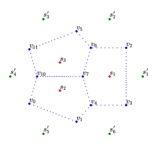
Figure 1. Paths for $C\colon y^{2}=x^{3}-x-1$. The dots marking the edges indicate the step size used for the certified homotopy continuation.

We describe generators of the fundamental group of $\mathbb{C}-S$ by cycles in a planar graph that we build in the following way.

We approximate the circle with centre $c_{0}=\frac{1}{\#S}\sum_{s\in S}s$ and radius $2\max_{s\in S}|s-c_{0}|$ using a regular polygon with vertices, say, $s_{1}^{\prime},\ldots,s_{6}^{\prime}$. Then we compute the Voronoi cell decomposition (see e.g. [Aurenhammer1991]) of $\mathbb{C}$ with respect to $S^{\prime}=S\cup\{s_{1}^{\prime},\ldots,s_{6}^{\prime}\}$. This produces a finite set of vertices $V=\{v_{1},\ldots,v_{r}\}\subset\mathbb{C}$ and a set $E$ of line segments $e_{ij}$ between $v_{i},v_{j}\in V$ such that the regions

$$F_{s}=\{x\in\mathbb{C}:|x-s|\leq|x-s^{\prime}|\text{ for any }s^{\prime}\in S^{\prime}-\{s\}\}$$

have boundaries consisting of $e_{ij}$, together with some rays for unbounded regions. We define $F_{\infty}=\bigcup_{s\in S^{\prime}-S}F_{s}$. Then we see that $F_{s}$ for $s\in S_{\infty}$ has a finite boundary, giving a loop separating $s$ from the rest of $S_{\infty}$. See Figure 1 for an illustration of the resulting graph for the curve $C\colon y^{2}=x^{3}-x-1$. It illustrates the set $S={s_{1},s_{2},s_{3}}$, together with the additional points $s^{\prime}_{1},\ldots,s^{\prime}_{6}$, and the vertices $v_{0},\ldots,v_{11}$ and edges between them, bounding the Voronoi cells $F_{s}$.

Lemma 2.1.

1. The boundaries of the regions $F_{s}$ for $s\in S_{\infty}$ provide cycles that generate $\operatorname{H}^{1}(\mathbb{C}-S,\mathbb{Z})$.

2. The fundamental group $\pi_{1}(\mathbb{C}-S,v_{i})$ is generated by cycles in the graph $(V,E)$.

Proof.

The first claim follows because the boundaries exactly form loops around each individual point $s$. The second claim follows because the graph is connected. Hence, we can find paths that begin and end in $v_{i}$ and (because of the first claim) provide a simple loop around a point $s\in S_{\infty}$. ∎

2.2. Lifting the graph via homotopy continuation

Each of our vertices $v_{i}\in\mathbb{C}$ has exactly $n$ preimages $v_{i}^{(1)},\ldots,v_{i}^{(n)}$, determined by the $n$ distinct simple roots of the equation $f(v_{i},y)=0$. We can parametrize each edge $e_{ij}$ from our graph by $x(t)=(1-t)v_{i}+tv_{j}\text{ for }t\in[0,1]$. We lift $e_{ij}$ to paths $e_{ij}^{(1)},\ldots,e_{ij}^{(n)}$ using the branches $y^{(k)}(t)$ defined by

$$f(x(t),y^{(k)}(t))=0\text{ and }y^{(k)}(0)=y(v_{i}^{(k)}).$$

Since $e_{ij}$ stays away from the critical locus, the function $y^{(k)}(t)$ is well-defined by continuity. Moreover, it is analytic in a neighbourhood of $e_{ij}^{(k)}$.

Given $k$, we have $y^{(k)}(1)=v^{k^{\prime}}_{j}$ for some $k^{\prime}$. Hence, every edge $e_{ij}$ determines a permutation $\sigma_{ij}$ such that $\sigma_{ij}(k)=k^{\prime}$. The lifted edge $e^{(k)}_{ij}$ connects $v_{i}^{(k)}$ to $v_{k}^{(\sigma_{ij}(k))}$. We write $(V^{\prime},E^{\prime})$ for this lifted graph on $C(\mathbb{C})$. If we split up the path in sufficiently small steps, we can determine these permutations.

Lemma 2.2.

With the notation above and for given $i,j$, we can algorithmically determine a subdivision

$$0=t_{0}<t_{1}<t_{2}<\cdots<t_{m_{ij}}=1$$

and real numbers $\varepsilon_{0},\ldots,\varepsilon_{m_{ij}-1}$ such that for $t,m$ satisfying $t_{m}\leq t\leq t_{m+1}$, we have that $|y^{(k^{\prime})}(t)-y^{(k)}(t_{m})|<\varepsilon_{m}$ if and only if $k^{\prime}=k$.

Proof.

We construct the $t_{m},\varepsilon_{m}$ iteratively, starting with $m=0$. We set

$$\varepsilon_{m}=\frac{1}{3}\min\{|y^{(k_{1})}(t_{m})-y^{(k_{2})}(t_{m})|:k_{1}\neq k_{2}\}$$

Using [Kranich2016, Theorem 2.1], we can determine from $f(x(t),y)$, $\varepsilon$, and $x(t_{m})$ a value $\delta>0$ such that for values $t$ satisfying $t_{m}\leq t\leq t_{m}+\delta$ we have that $|y^{(k)}(t)-y^{(k)}(t_{m})|<\varepsilon_{m}$. It follows that we can set $t_{m+1}=\min(1,t_{m}+\delta)$. Inspection of the formulas for $\delta$ give us that if the distance of any critical point from the path is positive, then there is a finite $m$ such that $t_{m}=1$. ∎

Remark 2.3.

In Figure 1, the dots on the edges mark the sequence $x(t_{0}),x(t_{1}),\ldots,x(t_{m_{ij}})$. In particular, on the edge from $v_{7}$ to $v_{10}$ one can see that as the distance to the branch points $s_{2},s_{3}$ gets smaller, the step sizes are reduced accordingly.

Lemma 2.4.

Given $\varepsilon<\varepsilon_{m}$, $t$ with $t_{m}<t\leq t_{m+1}$, and $\widetilde{y}_{m}$ with $|\widetilde{y}_{m}-y^{(k)}(t_{m})|<\varepsilon$, we can use Newton iteration to compute $\widetilde{y}$ such that $|\widetilde{y}-y^{(k)}(t)|<\varepsilon$.

Proof.

We use Newton iteration to approximate a root of $f(t,y)$, with initial value $\widetilde{y}_{m}$. We are looking for the unique root that lies within a radius of $\varepsilon_{m}$ of the initial value. If at any point the Newton iteration process escapes this disk, or if the iteration does not converge sufficiently quickly, we insert the point $(t_{m}+t)/2$ and restart. We know that if Newton iteration converges to a value in the disk, it must be the correct value. Furthermore, continuity implies that convergence will occur if if $|t-t_{m}|$ is small enough. ∎

Since $x(t_{0})\notin S$ we can use standard complex root finding algorithms on $f(x(t_{0}),y)=0$, to find approximations $\widetilde{y}^{(k)}_{0}$ to any desired finite accuracy. We then use Lemma 2.4 iteratively to find an approximation $\widetilde{y}^{(k)}_{m}$ to $y^{(k)}(t_{m})$, for each $m=1,\ldots,m_{ij}$.

The Voronoi graph $(V,E)$ generates the fundamental group of $\mathbb{C}-S$, so the lifted graph $(V^{\prime},E^{\prime})$ generates the fundamental group of the unramified cover $C(\mathbb{C})-x^{-1}(S_{\infty})$, and therefore also of $C(\mathbb{C})$. We have assumed that $C$ is an absolutely irreducible algebraic curve, so the graph is connected.

Remark 2.5.

For computing integrals along $v_{ij}^{(k)}$ in Section 3.2, we store for each relevant edge $e_{ij}$ the vectors $\{(t_{m},\varepsilon_{m},\widetilde{y}^{(1)}_{m},\ldots,\widetilde{y}^{(n)}_{m}):m\in\{0,\ldots,m_{ij}\}\}$. With this information we can quickly, reliably, and accurately approximate $y^{(k)}(t)$ for $t\in[0,1]$ using Lemma 2.4.

2.3. Computing the monodromy of $C\to\mathbb{P}^{1}$

We do not need this in the rest of the paper, but a side effect of computing the lifted graph is that we can also compute the monodromy of the cover $C\to\mathbb{P}^{1}$. To any path in the Voronoi graph we associate a permutation by composing the permutations associated with the constituent edges. For example, to the path $p=(v_{1},v_{2},v_{3})$ we associate the permutation $\sigma_{p}=\sigma_{12}\sigma_{23}$ (assuming that our permutations act on the right). Choosing, say, $v_{1}$ as our base point, this provides us with a group homomorphism $\pi_{1}(\mathbb{C}-S,v_{1})\to\operatorname{Sym}(n)$. The image gives the group of deck transformations of the cover or, in terms of field theory, a geometric realization of the Galois group of the degree $n$ field extension of $\mathbb{C}(x)$ given by $\mathbb{C}(x)[y]/(f(x,y))$. In particular, by taking a path that forms a loop around a single point $s\in C\cup\{\infty\}$, we can obtain the local monodromy of $s$. The cycle type of the corresponding permutation gives the ramification indices of the fibre over $s$. In particular, if the permutation is trivial, then $C\to\mathbb{P}^{1}$ is unramified over $s$.

2.4. Symplectic homology basis

Figure 2. Examples of the intersection pairing

Since $C(\mathbb{C})$ is a Riemann surface, it is orientable and hence we have a symplectic structure on its first homology. The pairing on cycles can be computed in the following way. Suppose that $\alpha,\beta$ are two paths intersecting at $v_{0}^{(1)}$, and that $\alpha$ contains the segment $v_{1}^{(1)}\to v_{0}^{(1)}\to v_{2}^{(1)}$ and that $\beta$ contains the segment $v_{3}^{(1)}\to v_{0}^{(1)}\to v_{4}^{(1)}$. We define

$$\langle\alpha,\beta\rangle_{v_{0}^{(1)}}=\langle\alpha,\beta\rangle_{v_{0}^{(1)}}^{\text{in}}+\langle\alpha,\beta\rangle_{v_{0}^{(1)}}^{\text{out}},\text{ and }\langle\alpha,\beta\rangle=\sum_{v}\langle\alpha,\beta\rangle_{v},$$

where $\langle\alpha,\beta\rangle_{v_{0}^{(1)}}=0$ if $\alpha$ or $\beta$ do not pass through $v_{0}^{(1)}$, and otherwise

$$\langle\alpha,\beta\rangle_{v_{0}^{(1)}}^{\text{in}}= \begin{cases}0&\text{ if }v_{3}=v_{1}\text{ or }v_{3}=v_{2}\\ \frac{1}{2}&\text{ if $v_{1},v_{3},v_{2}$ are counterclockwise oriented around $v_{0}$}\\ -\frac{1}{2}&\text{ if $v_{1},v_{3},v_{2}$ are clockwise oriented around $v_{0}$,}\end{cases}$$

$$\langle\alpha,\beta\rangle_{v_{0}^{(1)}}^{\text{out}}= \begin{cases}0&\text{ if }v_{3}=v_{1}\text{ or }v_{4}=v_{2}\\ \frac{1}{2}&\text{ if $v_{1},v_{2},v_{4}$ are counterclockwise oriented around $v_{0}$}\\ -\frac{1}{2}&\text{ if $v_{1},v_{2},v_{4}$ are clockwise oriented around $v_{0}$}.\end{cases}$$

At vertices where $\alpha,\beta$ meet transversely, this is clearly the usual intersection pairing on $H_{1}(C(\mathbb{C}),\mathbb{Z})$. A deformation argument verifies that the half-integer weights extend it properly to cycles with edges in common.

Lemma 2.6.

By applying an algorithm by Frobenius [Frobenius1879, §7] we can find a $\mathbb{Z}$-basis $\alpha_{1},\ldots,\alpha_{g},\beta_{1},\ldots,\beta_{g}$ for $\operatorname{H}_{1}(C(\mathbb{C}),\mathbb{Z})$ such that $\langle\alpha_{i},\alpha_{j}\rangle=\langle\beta_{i},\beta_{j}\rangle=0$ and $\langle\alpha_{i},\beta_{j}\rangle=\delta_{ij}$.

Proof.

We first compute a cycle basis for the lifted graph $(V^{\prime},E^{\prime})$ described in Section 2.2, say $\gamma_{1},\ldots,\gamma_{r}$ and compute the antisymmetric Gram matrix $G_{\gamma}=(\langle\gamma_{i},\gamma_{j}\rangle)_{ij}$. Frobenius’s algorithm yields an integral transformation $B$ such that $BG_{\gamma}B^{T}$ is in symplectic normal form, i.e., a block diagonal matrix with $g$ blocks

$$\begin{pmatrix}0&d_{i}\\ -d_{i}&0\end{pmatrix},$$

possibly followed by zeros, with $d_{1}\mid d_{2}\mid\cdots\mid d_{g}$. Because $C(\mathbb{C})$ is a complete Riemann surface, we know that $d_{1}=\cdots=d_{g}=1$ and that $g$ is the genus of $C(\mathbb{C})$. The matrix $B$ gives us $\alpha_{1},\beta_{1},\ldots,\alpha_{g},\beta_{g}$ as $\mathbb{Z}$-linear combinations of our initial cycle basis $\gamma_{1},\ldots,\gamma_{r}$. ∎

3. Computing the period lattice

3.1. A basis for $\operatorname{H}^{0}(C,\Omega_{C}^{1})$

From the adjunction formula [ACGH1985] we know that $\operatorname{H}^{0}(C,\Omega_{C}^{1})$ is naturally a subspace of the span of

$$\left\{\frac{h\,dx}{\partial_{y}f(x,y)}:h=x^{i}y^{j}\text{ with }0\leq i,j\text{ and }i+j\leq n-3\right\}.$$

If the projective closure of $\widetilde{C}$ is nonsingular, then $\operatorname{H}^{0}(C,\Omega_{C}^{1})$ is exactly this span. If $\widetilde{C}$ has only singularities at the projective points $(1:0:0),(0:1:0),(0:0:1)$ then Baker’s theorem [Baker1893] states that we can take those $(i,j)$ for which $(i+1,j+1)$ is an interior point to the Newton polygon of $f(x,y)$. In even more general situations, the adjoint ideal [ACGH1985, A§2] specifies exactly which subspace of polynomials $g$ corresponds to the regular differentials on $C$. We use Baker’s theorem when it applies and otherwise rely on Singular [DGPS] to provide us with a basis

$$\left\{\omega_{i}=\frac{h_{i}dx}{\partial_{y}f(x,y)}:i=1,\ldots,g\right\}\subset\operatorname{H}^{0}(C,\Omega_{C}^{1}).$$

3.2. Computing the period matrix

Given a basis $\omega_{1},\ldots,\omega_{g}$ for $\operatorname{H}^{0}(C,\Omega_{C}^{1})$ and a symplectic basis $\alpha_{1},\ldots,\alpha_{g},\beta_{1},\ldots,\beta_{g}$ for $\operatorname{H}_{1}(C(\mathbb{C}),\mathbb{Z})$, the corresponding period matrix is

$$\Omega_{\alpha\beta}=\left(\Omega_{\alpha}|\Omega_{\beta}\right)=\left(\int_{\alpha_{j}}\omega_{i}\,\right|\,\left.\int_{\beta_{j}}\omega_{i}\right)_{ij}.$$

The resulting period lattice is the $\mathbb{Z}$-span $\Lambda=\Omega_{\alpha\beta}\mathbb{Z}^{2g}$ of the columns in $\mathbb{C}^{g}$. As an analytic space, the Jacobian of $C$ is isomorphic to the complex torus $\mathbb{C}^{g}/\Lambda$. Our paths consist of lifted line segments, so we numerically approximate the integrals along the edges $e_{ij}^{(k)}$ that occur in our symplectic basis and compute $\Omega_{\alpha\beta}$ by taking the appropriate $\mathbb{Z}$-linear combinations of these approximations. To lighten notation we describe the process for the edge $e_{12}^{(1)}$. As in Section 2.2 we parametrize the edge by

$$x(t)=(1-t)v_{1}+tv_{2}$$

and with the stored information (see Remark 2.5), we can quickly compute $y^{(k)}(t)$ for given values of $t$. We obtain

$$\int_{e_{12}^{(1)}}\omega_{i}=(v_{2}-v_{1})\int_{t=0}^{1}\frac{h_{i}(x(t)y(t))}{\partial_{y}f(x(t),y(t))}dt.$$

Note that our integrand is holomorphic, so well suited for high order integration schemes such as Gauss-Legendre and Clenshaw-Curtis. We implemented Gauss-Legendre with relatively naive node computation. While in our experiments this was sufficient, there is the theoretical drawback that for very high order approximations, the determination of the integration nodes becomes the dominant part. There are sophisticated methods for obtaining the nodes with a better complexity (see [bogaert]). Alternatively, quadrature schemes like Clenshaw-Curtis may need more evaluation nodes to obtain the same accuracy, but allow for faster computation of these nodes.

Rather than compute guaranteed bounds, we have settled on a standard error estimation scheme, as described in, for instance, [BaileyEA2005, Section 5] to adapt the number of evaluation nodes. Since our applications will not provide proven results anyway, this is sufficient for our purposes.

Remark 3.1.

There is a split in literature on how to order the symplectic basis for the period matrix. With the normalization we use, one gets that

$$\Omega_{\alpha}^{-1}\Omega_{\alpha\beta}=(1\,|\,\Omega_{\alpha}^{-1}\Omega_{\beta})=(1\,|\,\tau)$$

where $\tau$ is a Riemann matrix, i.e., a symmetric matrix with positive definite imaginary part. Here $\tau$ represents the corresponding lattice in Siegel upper half space. In [birkenhake-lange], the period matrix is taken to be $\Omega_{\beta\alpha}$.

4. Homomorphism and isomorphism computations

4.1. Computing homomorphisms between complex tori

Let $C_{1}$ and $C_{2}$ be two curves with Jacobians $J_{1}$ and $J_{2}$. Let $\Omega_{1},\Omega_{2}$ be period matrices such that $J_{1}(\mathbb{C})=\mathbb{C}^{g_{1}}/\Omega_{1}\mathbb{Z}^{2g_{1}}$ and $J_{2}(\mathbb{C})=\mathbb{C}^{g_{2}}/\Omega_{2}\mathbb{Z}^{2g_{2}}$ as analytic groups.

A homomorphism $\phi\colon J_{1}\to J_{2}$ induces a tangent map $\operatorname{H}^{0}(C_{1},\Omega_{C_{1}}^{1})^{*}\to\operatorname{H}^{0}(C_{2},\Omega^{1}_{C_{2}})^{*}$ and a map on homology $\operatorname{H}_{1}(C_{1},\mathbb{Z})\to\operatorname{H}_{1}(C_{2},\mathbb{Z})$. After a choice of bases, these correspond to matrices $T=T_{\phi}\in M_{g_{2},g_{1}}(\mathbb{C})$ and $R=R_{\phi}\in M_{2g_{2},2g_{1}}(\mathbb{Z})$, which we call the tangent representation and the homology representation of $\phi$.

Proposition 4.1.

Let $\phi\colon J_{1}\to J_{2}$ be a homomorphism and let $T$, $R$ be the induced matrices described above.

1. The matrices $T=T_{\phi}$ and $R=R_{\phi}$ satisfy $T\Omega_{1}=\Omega_{2}R$.

2. A pair $(T,R)$ as in (i) comes from a uniquely determined homomorphism $\phi\colon J_{1}\to J_{2}$.

3. Either of the elements $T$ and $R$ in (i) is determined by the other.

4. If the curves $C_{1}$ and $C_{2}$ as well as the chosen bases of differentials and $\phi$ are defined over $k\subset\overline{\mathbb{Q}}$, then the matrix $T$ is an element of $M_{g_{2},g_{1}}(k)$.

Proof.

These results are in [birkenhake-lange, §1.2]. Writing $\overline{\Omega}_{2}$ for the element-wise complex conjugate of $\Omega_{2}$, we remark for part (iii) that we can determine $R$ from $T$ by considering

(4.2) $$\begin{pmatrix}T\Omega_{1}\\ \overline{T\Omega}_{1}\end{pmatrix}=\begin{pmatrix}\Omega_{2}\\ \overline{\Omega}_{2}\end{pmatrix}R,$$

since the first matrix on the right hand side of (4.2) is invertible. Conversely, we can determine $T$ from $R$ by considering the first $g_{1}$ columns on either side of $T\Omega_{1}=\Omega_{2}R$ since the corresponding matrices are invertible. ∎

We seek to recover these pairs $(T,R)$ numerically. This question was briefly touched upon in [ants-database, 6.1], and before that in [vanWamelen2006, §3], but here we give some more detail.

Lemma 4.3.

Given approximations of $\Omega_{1},\Omega_{2}$ to sufficiently high precision, we can numerically recover a $\mathbb{Z}$-basis for $\operatorname{Hom}(J_{1},J_{2})$, represented by matrices $R\in M_{2g_{2},2g_{1}}(\mathbb{Z})$ and $T\in M_{g_{2},g_{1}}(\mathbb{C})$ as in Proposition 4.1.

Proof.

Following Remark 3.1, we can normalize $\Omega_{i}$ to be of the form $(1\,|\,\tau_{i})$. We write

$$R=\begin{pmatrix}D&B\\ C&A\end{pmatrix}\text{, where }D,B,C,A\in M_{g_{2},g_{1}}(\mathbb{Z}).$$

Then $T=D+\tau_{2}C$, and

$$B+\tau_{2}A=(D+\tau_{2}C)\tau_{1}.$$

Considering real and imaginary parts separately, we obtain $m=2g_{1}g_{2}$ equations with real coefficients in $n=4g_{1}g_{2}$ integer variables, denoted by $M\in M_{m,n}(\mathbb{R})$. We recognize integer solutions that are small compared to the precision to which we calculated $\tau_{1},\tau_{2}$ in the following way. Observe that such solutions correspond to short vectors in the lattice generated by the columns of $(I\mid\varepsilon^{-1}M)$, where $\varepsilon$ is some small real number. The LLL algorithm can find such vectors, and we keep the ones that lie in the kernel to the specified precision.

If sufficient precision is used, then we obtain a basis for $\operatorname{Hom}(J_{1},J_{2})$ in this way. (Heuristically, any approximation to high precision will do.) Proposition 4.1 shows how to recover the tangent representation $T$ from the corresponding homology representations $R$. ∎

Remark 4.4.

An important tuning parameter for applications of LLL is the precision. We have an (estimated) accuracy of the entries in the matrix $M$. We choose $\varepsilon$ such that $\varepsilon^{-1}M$ has accuracy to within $0.5$. If we have computed the period matrices to a precision of $b$ bits, then $M$ contains about $2g_{1}g_{2}b$ bits of information. We would therefore expect that the entries in the LLL basis have entries of size about $(2g_{1}g_{2}b)/(4g_{1}g_{2})=b/2$. We only keep vectors that have entries of bit-size at most half that.

In the context of Proposition 4.1(iv), the algebraic entries of $T$ can be recognized by another application of the LLL algorithm; for example, the SageMath implementation
number_field_elements_from_algebraics can be used to this end. We emphasize that in order to recover this algebraicity, we need the original period matrices $\Omega_{i}$ with respect to a basis of $H^{0}(C,\Omega^{1}_{C})$ defined over $\overline{\mathbb{Q}}$. A differential basis for which the period matrix takes the shape $(1\,|\,\tau_{i})$ usually has a transcendental field of definition.

For a Jacobian $J$, the natural principal polarization gives rise to the Rosati-involution on $\operatorname{End}(J)$ (cf. [birkenhake-lange, §5.1]). We choose a symplectic basis for $H_{1}(C(\mathbb{C}),\mathbb{Z})$ and denote the standard symplectic form by

$$E=\begin{pmatrix}0&I\\ -I&0\end{pmatrix}\in M_{2g,2g}(\mathbb{Z}).$$

Proposition 4.5.

Let $\phi\colon J\to J$ be an endomorphism with corresponding pair $(T,R)$ as in Proposition 4.1(i). Then the Rosati involution $\phi^{\dagger}$ of $\phi$ corresponds to the pair $(T^{\dagger},R^{\dagger})$ with

$$R^{\dagger}=-ER^{t}E.$$

Proof.

Since we chose our homology basis to be symplectic, the Rosati involution of the endomorphism corresponding to $R$ corresponds to the adjoint with respect to the pairing defined by $E$, which is $ER^{t}E^{-1}=-ER^{t}E$. ∎

Remark 4.6.

Proposition 4.1(iii) shows how to obtain $T^{\dagger}$ from $R^{\dagger}$.

Recall [birkenhake-lange, Chapter 5] that any polarized abelian variety allows a decomposition up to isogeny

(4.7) $$J\sim\prod_{i}A_{i}^{e_{i}}$$

into powers of simple polarized quotient abelian varieties $A_{i}$.

Corollary 4.8.

Let $J$ be the Jacobian of a curve $C$, and let $\Omega$ be a corresponding period matrix. If we know $\Omega$ to sufficiently high precision, then we can numerically determine the factors in (4.7). Furthermore, if $J$ is defined over $\overline{\mathbb{Q}}$, we can numerically determine a field of definition for each of the conjectural factors $A_{i}$.

Proof.

Using Lemma 4.3 we can compute generators for $\operatorname{End}(J)$. We can then determine symmetric idempotent matrices $e\in M_{2g,2g}(\mathbb{Q})$ by using meataxe algorithms, or alternatively by directly solving $e^{2}=e$ in the subring of $\operatorname{End}(J)$ fixed by the Rosati involution. The columns of $\Omega e$ span a complex torus of smaller dimension. By [KaniRosen1989] all isogeny factors of $J$ occur this way.

In order to find a field of definition, we can determine the matrix $T$ corresponding to $e$ and recognize its entries as algebraic numbers. Then [KaniRosen1989] shows that the image of the projection $T$ is still polarized, and defined over the corresponding field. ∎

4.2. Computing symplectic isomorphisms

When $g_{1}=g_{2}$, Lemma 4.3 allows us to recover possible isomorphisms between $J_{1}$ and $J_{2}$, as these correspond to the matrices $R$ with $\det(R)=\pm 1$.

In particular, this gives us a description of the automorphism group of a Jacobian variety $J$ as the subgroup of elements of $\operatorname{End}(J)$ with determinant $1$. This group can be infinite. However, note that we have principal polarizations on $J_{1}$ and $J_{2}$. We take symplectic bases for the homology of both Jacobians, and let $\alpha:J_{1}\to J_{2}$ be an isomorphism, represented by $R\in M_{2g,2g}(\mathbb{Z})$.

Definition 4.9.

We say that $\alpha$ is symplectic if we have $R^{t}E_{2}R=E_{1}$.

Remark 4.10.

More intrinsically, the definition demands that the canonical intersection pairings $E_{1}$ and $E_{2}$ on on $\operatorname{H}_{1}(C_{1},\mathbb{Z})$ and $\operatorname{H}_{1}(C_{2},\mathbb{Z})$ satisfy $\alpha^{*}E_{2}=E_{1}$.

The symplectic automorphisms of $J$ form a group, which is called the symplectic automorphism group $\operatorname{Aut}(J,E)$ of the principally polarized abelian variety $(J,E)$.

Theorem 4.11.

Suppose that $C$ is a smooth curve of genus at least $2$. Then we have the following.

1. The symplectic automorphism group of $J$ is finite.

2. There is a canonical map $\operatorname{Aut}(C)\to\operatorname{Aut}(J,E)$. If $C$ is non-hyperelliptic, then this map is an isomorphism; otherwise it induces an isomorphism $\operatorname{Aut}(C)\stackrel{{\scriptstyle\sim}}{{\to}}\operatorname{Aut}(J,E)/\langle-1\rangle$.

Proof.

Part (i) is [birkenhake-lange, 5.1.9], and (ii) is the Torelli theorem [Milne1986, Theorem 12.1]. ∎

This shows we can recover $\operatorname{Aut}(C)$ from $\operatorname{Aut}(J,E)$. In fact, from the linear action of the symplectic automorphism on $H^{0}(C,\Omega^{1}_{C})^{*}$ we can recover its action on a canonical model of $C$ in $\mathbb{P}H^{0}(C,\Omega^{1}_{C})^{*}$. For non-hyperelliptic curves this realizes the isomorphism $\operatorname{Aut}(J,E)/\langle-1\rangle\simeq\operatorname{Aut}(C)$ explicitly. For hyperelliptic curves it recovers the reduced automorphism group, which can in fact be determined more efficiently by purely algebraic methods, as described in [lrs-ants].

If $C$ is defined over $\overline{\mathbb{Q}}$, then we can verify that the numerical automorphisms thus obtained are correct by working purely algebraically: by Proposition 4.1(iv) we obtain an algebraic expression for $T$. We can then check by exact calculation that it fixes the defining ideal of the canonical embedding of $C$.

More generally, given two Jacobians $J_{1}$ and $J_{2}$, we can determine the numerical symplectic isomorphisms between them. To this end, one proceeds as in the proof of [birkenhake-lange, 5.1.8]: we have

(4.12) $$R^{t}E_{2}R=E_{1}$$

or

(4.13) $$(E_{1}^{-1}R^{t}E_{2})R=1.$$

In particular, we get

(4.14) $$\operatorname{tr}((E_{1}^{-1}R^{t}E_{2})R)=2g$$

for the common genus $g$ of $C_{1}$ and $C_{2}$. Let $B=\left\{B_{1},\dots,B_{d}\right\}$ be a $\mathbb{Z}$-basis of $\operatorname{Hom}(J_{1},J_{2})$. Then we can write

(4.15) $$R=\sum_{i=1}^{d}\lambda_{i}B_{i}.$$

The positivity of the Rosati involution implies that the set of solutions $\lambda_{1},\dots,\lambda_{d}$ of (4.14) is finite. Explicitly, these can be obtained by using the Fincke-Pohst algorithm [fincke-pohst]. For the finite set of solutions thus obtained, we check which yield matrices $R$ in (4.15) that numerically satisfy (4.13). These matrices constitute the homology representations $R$ of numerical isomorphisms $J_{1}\to J_{2}$. From this, we can obtain the corresponding tangent representations $T$ by Proposition 4.1(iii), and we can verify these algebraically as above.

Remark 4.16.

Using the same methods, one can determine the maps $C_{1}\to C_{2}$ of a fixed degree $d$ by finding the $\alpha$ for which $\alpha_{*}E_{1}=dE_{2}$. This is especially useful if the genus $g_{2}$ of $C_{2}$ is larger than $2$, since then we can bound $d$ by $(2g_{1}-2)/(2g_{2}-2)$.

In this way, we obtain the following pseudocode.

Algorithm Compute isomorphisms between curves.

Input: Planar equations $f_{1},f_{2}$ for two curves $C_{1},C_{2}$, as well as a given working precision.

Output: A numerical determination of the set of isomorphisms $C_{1}\to C_{2}$.

1. Check if $g(C_{1})=g(C_{2})$; if not, return the empty set;

2. Check if $C_{1}$ and $C_{2}$ are hyperelliptic; if so, use the methods in [lrs-ants];

3. Otherwise, determine the period matrices $P_{1},P_{2}$ of $C_{1},C_{2}$ to the given precision, using the algorithm in the introduction;

4. Using Lemma 4.3 (see also [ants-database, 6.1]), determine a $\mathbb{Z}$-basis of $\operatorname{Hom}(J_{1},J_{2})\subset M_{2g,2g}(\mathbb{Z})$ represented by integral matrices $R\in M_{2g,2g}(\mathbb{Z})$;

5. Using Fincke-Pohst, determine the finite set $S=\left\{R\in\operatorname{Hom}(J_{1},J_{2})\mid\operatorname{tr}((E_{1}^{-1}R^{t}E_{2})R)=2g\right\}$;

6. Using the canonical morphisms with respect to the chosen bases of differentials, return the subset of elements of $S$ that indeed induce an isomorphism $C_{1}\to C_{2}$.

5. Examples

The examples in this section can be found online at [GitHub].

Example 5.1.

Consider the curve

$$C:4x^{6}-54x^{5}y-729x^{4}+108x^{3}y^{3}+39366x^{2}-54xy^{5}-531441.$$

This is a non-hyperelliptic curve of genus $6$. Theorem 4.11 shows that, at least numerically, its geometric automorphism group is of order $2$ and generated by the involution $\iota:(x,y)\mapsto(-x,-y)$. Lemma 4.3 shows that its numerical geometric endomorphism ring is of index $6$ in $\mathbb{Z}\times\mathbb{Z}\times\mathbb{Z}$.

The quotient of $C$ by its automorphism group gives a morphism of degree $2$ to the genus $2$ curve

$$D_{1}:y^{2}=x^{6}-x^{5}+1.$$

This corresponds to the symmetric idempotent $e_{1}=1-(1+\iota)/2$ in the endomorphism algebra, whose tangent representation has numerical rank $4$. Numerically, there are two other such symmetric idempotents $e_{2}$, $e_{3}$. Together, their kernels span $\operatorname{H}_{1}(C(\mathbb{C}),\mathbb{Z})$, and all of these are of dimension $4=2\cdot 2$. This means that along with $A_{1}=\operatorname{Jac}(D_{1})$ there should be two other $2$-dimensional abelian subvarieties $A_{2}$, $A_{3}$ of $\operatorname{Jac}(C)$ such that

$$\operatorname{Jac}(C)\sim A_{1}\times A_{2}\times A_{3}.$$

We now describe the abelian varieties $A_{2}$ and $A_{3}$.

The tangent representation of an idempotent $e_{i}$ corresponding to a factor $A_{i}$ has dimension $4$. Its kernel is therefore a subspace $W_{i}$ of $\operatorname{H}^{0}(C,\Omega_{C}^{1})$ of dimension $2$. If the idempotent $e_{i}$ is induced by a map of curves $p:C\to D_{i}$, then $W_{i}=p^{*}\operatorname{H}^{0}(D_{i},\Omega_{D_{i}}^{1})$ for some curve $D_{i}$ and some projection $p\colon C\to D_{i}$.

By composing the canonical map with the projection to the projective line $\mathbb{P}W_{i}$, all the idempotents $e_{i}$ give rise to a cover $C\to\mathbb{P}W_{i}$. Now if $e_{i}$ is induced by a projection $C\to D_{i}$ at all, then $D_{i}$ is a subcover of this map $C\to\mathbb{P}W_{i}$. It turns out that all $e_{i}$ give rise a subcover of the degree $6$ non-Galois cover

$$C \to\mathbb{P}^{1}$$

$$(x,y) \to y/x.$$

A monodromy calculation gives the Galois closure $Z\to\mathbb{P}^{1}$ of this cover: its Galois group $G$ is dihedral of order $12$. In particular, considering the subgroups of $G$ that properly contain the degree $2$ subgroup corresponding to $C\to\mathbb{P}^{1}$, we see that there exist exactly two non-trivial subcovers $p_{1}\colon C\to D_{1}$ and $p_{2}\colon C\to D_{2}$ of $C\to\mathbb{P}^{1}$. These subcovers have degree $2$ and degree $3$, respectively.

The curves $D_{1}$ and $D_{2}$ are both of genus $2$. The first subcover $p_{1}$ is a quotient of $C$ and corresponds to the curve $D_{1}$ above. The second subcover $p_{2}$ is not a quotient of $C$, but using Galois theory for the normal closure still furnishes us with a defining equation of $D_{2}$, namely

$$D_{2}\colon y^{2}=-16x^{5}-40x^{4}+32x^{3}+88x^{2}-32x-23.$$

We take $A_{2}$ to be the Jacobian of $D_{2}$.

Since we have exhausted all subcovers of the Galois closure $Z\to\mathbb{P}^{1}$, we conclude that $A_{3}$ does not arise from a cover $C\to D_{3}$. Still, using analytic methods we find that numerically the subvariety $A_{3}$ is simple and admits a (unique) principal polarization. It is therefore the Jacobian of a curve $D_{3}$ of genus $2$. Calculating the Igusa invariants numerically, we reconstruct

$$D_{3}\colon y^{2}=x^{6}+3x^{4}+3x^{2}+x+1.$$

We can numerically check that there is a morphism of abelian varieties $\operatorname{Jac}(C)\to\operatorname{Jac}(D_{3})$ that is compatible with the polarizations on both curves. A computation on homology again shows that this morphism cannot come from a morphism of curves $C\to D_{3}$; if it did, the degree of such a morphism would have to be $6$, which is impossible in light of the Riemann-Hurwitz formula. An explicit correspondence between $C$ and $D_{3}$ can in principle be found by using the methods in [CMSV]; however, this will still be a rather involved calculation, which we have therefore not performed yet.

Example 5.2.

Consider the plane model

$$C\colon f(x,y)=1+7xy+21x^{2}y^{2}+35x^{3}y^{3}+28x^{4}y^{4}+2x^{7}+2y^{7}=0$$

of the Macbeath curve from [hidalgo-macbeath], which is due to Bradley Brock. Its automorphism group is isomorphic to $\operatorname{PSL}_{2}(\mathbb{F}_{8})$ and has order $504$. We illustrate that the algorithm described in Section 4.2 indeed recovers that $\operatorname{Aut}(C)$ is isomorphic to $\operatorname{PSL}_{2}(\mathbb{F}_{8})$, that $C$ is indeed the Macbeath curve, and moreover that all the automorphisms of $C$ are already defined over the cyclotomic field $\mathbb{Q}(\zeta_{7})$.

From the adjoint ideal computed by Singular [DGPS] we find a $\mathbb{Q}$-rational basis of $7$ global differentials of the form $h\omega$, where $\omega=\frac{\partial f}{\partial y}dx$ and where $h$ is one of

$$\left\{h_{1},\dots,h_{7}\right\}=\{4x^{2}y^{2}+3xy+1,2y^{5}-x^{3}y-x^{2},2xy^{4}+x^{4}+y^{3},$$

$$4x^{2}y^{3}+3xy^{2}+y,4x^{3}y^{2}+3x^{2}y+x,2x^{4}y+y^{4}+x^{3},2x^{5}-xy^{3}-y^{2}\}.$$

We can determine a corresponding period matrix to binary precision $100$ after about a minute’s calculation, and find the corresponding numerical symplectic automorphism group. It indeed has cardinality $1008$, and its elements are well-approximated by relatively simple matrices in the cyclotomic field $\mathbb{Q}(\zeta_{7})$ that also generate a group $G\subset\operatorname{GL}_{7}(\mathbb{Q}(\zeta_{7}))$ of order $1008$ with $G\cap\mathbb{Q}(\zeta_{7})^{*}=\langle-1\rangle$ and with $G/\langle-1\rangle\cong\operatorname{PSL}_{2}(\mathbb{F}_{2}^{3})$. In practice this is of course indication enough that the automorphism group has been found.

To prove this, we choose two elements $T_{1},T_{2}$ of $G$. The first of these is the diagonal matrix with entries $\left\{1,\zeta_{7}^{2},\zeta_{7}^{4},\zeta_{7}^{6},\zeta_{7},\zeta_{7}^{3},\zeta_{7}^{5}\right\}$; the other has relatively modest entries but is still too large to write down here. We check that these matrices generate a subgroup of $G$ of cardinality $504$ that projects isomorphically to $G/\langle-1\rangle$. If we show that $T_{1}$ and $T_{2}$ indeed correspond to automorphisms of $C$, then our claims will be proved, since any curve of genus $7$ with (at least) $504$ automorphisms is birational to the Macbeath curve.

To verify this claim, one can use the canonical embedding of $C$ with respect to the given basis of global differentials $\left\{h_{i}\omega\right\}$. Alternatively, one observes that

$$x=h_{5}/h_{1},\,y=h_{4}/h_{1}.$$

This means that after applying one of the transformations $T_{1},T_{2}$ to the basis of global differentials to obtain the linear transformations $\left\{T_{i}(h_{j}\omega)\right\}_{j}$, we can recover corresponding transformations $x^{\prime}$ and $y^{\prime}$ in $x$ and $y$ via

$$x^{\prime}=T_{i}(h_{5}\omega)/T_{i}(h_{1}\omega),\,y^{\prime}=T_{i}(h_{4}\omega)/T_{i}(h_{1}\omega).$$

For $T_{1}$, we get

$$x^{\prime}=\zeta_{7}x,\,y^{\prime}=\zeta_{7}^{6}y,$$

while for $T_{2}$ we get two decidedly unpleasant rational expressions the degree of whose denominator and numerator both equal $5$. In either case, we can check that the corresponding substitutions leave the equation for $C$ invariant, which provides us with the desired verification of correctness of $T_{1}$ and $T_{2}$.

Example 5.3.

This example illustrates the value of being able to verify isogeny factors of Jacobians numerically. We consider a genus $4$ curve $C$ and an unramified double cover $\pi\colon D\to C$. Then $D$ is of genus $7$, and $\operatorname{Jac}(D)$ is isogenous to $\operatorname{Jac}(C)\times A$ for some $3$-dimensional abelian variety $A$. The theory of Prym varieties shows we can take $A$ to be principally polarized. It follows that generally $A$ is a quadratic twist of a Jacobian of a genus $3$ curve $F$. In [Milne1923] W.P. Milne constructs a plane quartic $F$ from a genus $4$ curve $C$ with data that amounts to specifying an unramified double cover of $C$. One would guess that $\operatorname{Jac}(F)$ is indeed the Prym variety of $D/C$. Here we check this numerically for a particular example. A modern, systematic treatment of this construction is in preparation [BHS].

Let $C$ be the canonical genus $4$ curve in $\mathbb{P}^{3}$, described by $\Gamma_{2}=\Gamma_{3}=0$, where

$$\Gamma_{2} =x^{2}+xy+y^{2}+3xz+z^{2}-yw+w^{2},\Gamma_{3} =xyz+xyw+xzw+yzw.$$

A plane model for this curve is given by

$$\begin{split}\widetilde{C}\colon y^{4}w^{2}-y^{3}w^{3}+y^{2}w^{4}+2y^{4}w-y^{3}w^{2}+2yw^{4}+y^{4}-2y^{2}w^{2}\\ +yw^{3}+w^{4}-y^{2}w-yw^{2}+y^{2}+2yw+w^{2}=0.\end{split}$$

Since $\Gamma_{3}$ has four nodal singularities in general position, it is a Cayley cubic. It admits a double cover unramified outside the nodes, obtained by adjoining the square root of the Hessian of $\Gamma_{3}$. Since $C$ does not pass through the nodes, this induces an unramified double cover $D$ of $C$. It is geometrically irreducible and admits a plane model

$$\begin{split}\widetilde{D}\colon u^{4}v^{4}-3u^{4}v^{2}+u^{4}-u^{3}v^{3}-2u^{3}v+u^{2}v^{2}-u^{2}+3uv^{3}+2uv+v^{4}+v^{2}+1=0.\end{split}$$

Milne’s construction yields a plane quartic

$$\begin{split}F\colon 5s^{4}+28s^{3}t+28s^{3}+47s^{2}t^{2}+76s^{2}t+44s^{2}+34st^{3}+82st^{2}\\ +66st+18s+16t^{4}+34t^{3}+32t^{2}+18t+1=0.\end{split}$$

Numerical computation shows that $\operatorname{End}(\operatorname{Jac}(C))=\mathbb{Z}$ and that $\operatorname{End}(\operatorname{Jac}(F))=\mathbb{Z}$, which can be confirmed by the $\ell$-adic methods in [CMSV]. It follows that $\operatorname{Hom}(\operatorname{Jac}(F),\operatorname{Jac}(C))=0$. Furthermore, we find that $\operatorname{Hom}(\operatorname{Jac}(C),\operatorname{Jac}(D))$ and $\operatorname{Hom}(\operatorname{Jac}(F),\operatorname{Jac}(D))$ are $1$-dimensional, so it follows that $\operatorname{Jac}(D)\sim\operatorname{Jac}(C)\times\operatorname{Jac}(F)$ and that $\operatorname{Jac}(F)$ lies in the Prym variety of the cover $D\to C$. Thus, we obtain numerical evidence that Milne indeed provides a construction of a curve $F$ generating the Prym variety.

Example 5.4.

This example is similar to Example 5.1, except that the curve has extra automorphisms, which allows a more direct identification of the factors. Consider the curve

$$C:3x^{5}+2x^{3}y^{2}-xy^{4}-9x^{4}+6x^{2}y^{2}-y^{4}+4=0$$

of genus $6$. Computing the canonical map shows that $C$ is non-hyperelliptic. Theorem 4.11 shows numerically that $\operatorname{Jac}(C)$ has a symplectic automorphism group that is dihedral of order $12$, which means the automorphism group of $C$ is isomorphic to $\operatorname{Sym}(3)$. From the tangent representation one can find that these numerically determined automorphisms act linearly on the affine model of $C$, and it is easy to recover exact representatives and verify that they are indeed automorphisms of $C$.

We compute the quotient of $C$ by each of the involutions. For the involution $(x,y)\mapsto(x,-y)$ this is particularly straightforward. For the other involution $(x,y)\mapsto(-\frac{1}{2}x+\frac{i}{2}y,-\frac{3i}{2}x+\frac{1}{2}y)$ and its quadratic conjugate it is slightly more work, but in all cases we find that the quotient is birational to

$$D_{1}:y^{2}=x^{6}-x^{5}+1.$$

We can compute numerically that the $\mathbb{Z}$-module of homomorphisms from $\operatorname{Jac}(D_{1})$ to $\operatorname{Jac}(C)$ is of rank $2$. The images span a rank $8$ submodule on the homology, indicating that $\operatorname{Jac}(D_{1})^{2}$ is an isogeny factor of $\operatorname{Jac}(C)$.

Similarly, the quotient of $C$ by the order $3$ group generated by $(x,y)\mapsto(-\frac{1}{2}x+\frac{i}{2}y,\frac{3i}{2}x-\frac{1}{2}y)$ yields

$$D_{2}:y^{2}=2x^{5}+27x^{4}-54x^{2}+27.$$

This provides us with sufficient information to conclude that

$$\operatorname{Jac}(C)\sim\operatorname{Jac}(D_{1})^{2}\times\operatorname{Jac}(D_{2}).$$

Both of the curves $D_{1}$ and $D_{2}$ have endomorphism ring $\mathbb{Z}$ over $\overline{\mathbb{Q}}$, as can be verified by the $\ell$-adic methods in [CMSV]. Similar considerations show that the Jacobians of $D_{1}$ and $D_{2}$ are not isogenous. Therefore the numerical endomorphism ring of $\operatorname{Jac}(C)$ is an order in $\mathbb{Q}\times M_{2}(\mathbb{Q})$; closer consideration of the representation of the action of its generators on homology obtained by Lemma 4.3 shows that it is of index $9$ in $\mathbb{Z}\times M_{2}(\mathbb{Z})$.

Appendix A Guide to implementation

We briefly describe how the implementation of our routines in SageMath can be used. For the sake of brevity, we limit ourselves to genus $1$ and $2$ curves here, but obviously our implementations mainly provide novel capabilities for higher genus curves.

The basic data structure is most easily accessed by defining a plane algebraic curve. The most important attribute at this point is specifying the numerical working precision (in bits).

sage: A2.<x,y>=AffineSpace(QQ,2)
sage: E=Curve(x^3+y^3+1)
sage: SE=E.riemann_surface(prec=60)

The various attributes and routines of the complex torus derived from the Riemann surface SE can be accessed via methods on the object. For instance, we can (numerically) compute a $\mathbb{Z}$-basis for the homomorphisms, represented by matrices $R$ acting on the homology. There are parameters available to tune the use of LLL to recognize actual endomorphisms, but some care is taken to choose reasonable defaults based on the precision available.

sage: Rs=SE.symplectic_isomorphisms(SE);Rs
[ [ 0 -1]  [ 1  1]  [1 0]  [ 0  1]  [-1 -1]  [-1  0]
  [ 1  1], [-1  0], [0 1], [-1 -1], [ 1  0], [ 0 -1] ]

In simple cases such as this one we can recognize the algebraic matrices acting on the tangent space (SageMath here chooses to express things in a sixth root of unity).

sage: Ts=SE.tangent_representation_algebraic(A);Ts
[[a], [-a + 1], [1], [-a], [a - 1], [-1]]
sage: Ts[0]^3
[-1]

The Jacobian of the following genus $2$ curve has $E$ as an isogeny factor.

sage: C=HyperellipticCurve(X^6 + 3*X^4 + 3*X^2 + 2)
sage: SC=C.riemann_surface(prec=60)
sage: SC.homomorphism_basis(SE)
[ [ 0  0  1 -1]  [-1  1  0  0]
  [-1  1 -1  1], [ 0  0 -1  1] ]

We can identify the cofactor as well.

sage: SE2=EllipticCurve([1,0]).riemann_surface(prec=60)
sage: SC.homomorphism_basis(SE2)
[ [ 1  1 -1 -1]  [ 0  0  1  1]
  [ 0  0  1  1], [-2 -2  0  0] ]