Time-Delay Interferometry and Clock-Noise Calibration

Abstract

The Laser Interferometer Space Antenna is a joint ESA-NASA space-mission to detect and study mHz cosmic gravitational waves. The trajectories followed by its three spacecraft result in unequal- and time-varying arms, requiring use of the Time-Delay Interferometry (TDI) post-processing technique to cancel the laser phase noises affecting the heterodyne one-way Doppler measurements. Although the second-generation formulation of TDI cancels the laser phase noises when the array is both rotating and “flexing”, second-generation TDI combinations for which the phase fluctuations of the onboard ultra stable oscillators (USOs) can be calibrated out have not appeared yet in the literature. In this article we present the solution of this problem by generalizing to the realistic LISA trajectory the USO calibration algorithm derived by Armstrong, Estabrook and Tinto for a static configuration.

I Introduction

Gravitational waves (GWs) are predicted by Einstein’s theory of general relativity and represent disturbances of space-time propagating at the speed of light. Because of their extremely small amplitudes and interaction cross-sections, GWs carry information about regions of the Universe that would be otherwise unobtainable through the electromagnetic spectrum. Their first detection announced by the LIGO project in February 2016 Abbott and et al (2016a), followed by the additional observations of four more events Abbott and et al (2016b, 2017a, 2017b, 2017c), mark the beginning of GW Astronomy.

Contrary to ground-based laser interferometers, which are sensitive to GWs in a band from about a few tens of Hz to a few kilohertz, space-based interferometers are expected to access the frequency region from a few tenths of millihertz to about a few tens of Hz, where GW signals are expected to be larger in number and characterized by larger amplitudes. The most notable example of a space-based interferometer, which for several decades has been jointly studied in Europe and in the United States of America, is the Laser Interferometer Space Antenna (LISA) mission Amaro-Seoane and et al (2017). LISA, which is now expected to be launched in the year 2034, will detect and study cosmic gravitational waves in the $10^{-4}-1$ Hz band by relying on coherent laser beams exchanged by three remote spacecraft along the arms of their forming giant (almost) equilateral triangle of $2.5\times 10^{6}$ km arm-length.

A space-based laser interferometer GW detector measures relative frequency changes experienced by coherent laser beams exchanged by three pairs of spacecraft. As the laser beams are received, they are made to interfere with the outgoing laser light. Since the received and receiving frequencies of the laser beams can be different by tens to perhaps hundreds of MHz (consequence of the Doppler effect from the relative inter-spacecraft velocities and the intrinsic frequency differences of the lasers), to remove these large beat-notes present in the heterodyne measurements one relies on the use of a microwave signal generated by an onboard clock (usually referred to as Ultra-Stable Oscillator (USO)). The magnitude of the frequency fluctuations introduced by the USO into a heterodyne one-way Doppler measurement depends linearly on the USO’s noise itself and the heterodyne beat-note frequency. Space-qualified, state of the art clocks are oven-stabilized crystals characterized by an Allan standard deviation of ${\sigma_{A}}\approx 10^{-13}$ for averaging times in the interval $1-10^{4}$ s, covering the frequency band of interest to space-based interferometers Amaro-Seoane and et al (2017). In the case of the LISA mission, in particular, it was estimated Tinto et al. (2002) that the magnitude of the square-root of the power spectral density of the USO’s relative frequency fluctuations appearing, for instance, in the unequal-arm Michelson TDI combination $X$ (valid for a static-array configuration) would be about three orders of magnitude larger than that due to the residual (optical path and proof-mass) noise sources.

A technique for removing the USO noise from a Michelson interferometer for a static array configuration was first discussed in Hellings et al. (1996), applied in Hellings (2001) to the unequal-arm Michelson $X$ and Sagnac $\alpha$ TDI combinations for a static array (TDI-1) and improved and extended to all the TDI-1 combinations in Tinto et al. (2002). This technique requires the modulation of the laser beams exchanged by the spacecraft, and the further measurement of six more inter-spacecraft relative phases by comparing the sidebands of the received beam against sidebands of the transmitted beam. The physical reason behind the use of modulated beams for calibrating the USOs noises is to exchange the USOs phase fluctuations with the same time delays as those experienced by the laser phase noises as they propagate along the three arms. By performing sideband-sideband measurements Hellings et al. (1996); Hellings (2001); Tinto et al. (2002) six additional one-way phase differences are generated that allow one to calibrate out the USOs phase fluctuations from the TDI-1 combinations while preserving the gravitational wave signal in the resulting USO-calibrated TDI data.

Although an alternative experimental implementation to the modulation technique has recently been proposed Tinto and Yu (2015), which relies on the use of an onboard optical-frequency comb Hall (2006); Hänsch (2006); Giunta et al. (2016) to generate the microwave frequency coherent to the frequency of the onboard laser , in this article we derive the TDI combinations for a rotating and “flexing” array (so called second-generation TDI, TDI-2) that calibrate out the microwave signal phase fluctuations due to the onboard LISA USOs. A summary of this article is presented below.

In Section II we provide the mathematical expressions describing the one-way heterodyne measurements performed onboard the LISA spacecraft. They reflect the planned LISA’s split-interferometry design, and they were first presented in Otto et al. (2012). There Otto et al also proposed a data processing algorithm to obtain TDI-2 combinations that are USO noise-free. Their approach, however, has recently been shown (by the LISA Simulation Working Group) to not work as expected and we discuss the physical reasons behind its short-coming.

After showing that the commutator of two delay-operators applied to the phase noise of a LISA USO results in relative frequency fluctuations (strain) that are significantly smaller than those associated with the acceleration and optical-path noises, in Section III we derive the expressions that calibrate the USO noises out of the TDI-2 unequal-arm Michelson and Sagnac interferometric combinations Tinto and Dhurandhar (2014). A summary of our results and conclusions are then presented in Section IV.

II Split-Interferometry One-Way Heterodyne Measurements

In what follows we provide the expressions for the eight one-way heterodyne measurements performed onboard spacecraft # $1$; the remaining $16$ can be obtained by cyclic permutation of the spacecraft indices. These expressions were discussed in Otto et al. (2012) in the context of the LISA split-interferometry architecture and we refer the reader to that publication for more details. Here we modify those expressions by multiplying both sides of the equations given there by the functions $\theta_{ij}$, which are either equal to $+1$ or $-1$ depending on whether the frequency of the received beam, $\nu_{i}$, is larger or smaller than the frequency $\nu_{j}$ of the receiving beam respectively. This results in modified expressions for the fractional frequency beat-note coefficients, which are given below.

We adopt the description of the LISA array given in Tinto and Dhurandhar (2014), in which the beam arriving at spacecraft $i$ has subscript $i$ and is primed or unprimed depending on whether the beam is traveling respectively clockwise or counter-clockwise around the LISA triangle as seen from above the plane of the constellation described in Fig. (1). We also adopt the usual notation for delayed data streams, which is convenient for algebraic manipulations Tinto and Dhurandhar (2014). We define the six time-delay operators ${\cal D}_{i}$, ${\cal D}_{i^{\prime}}$, $i=1,2,3\ ,\ i^{\prime}=1^{\prime},2^{\prime},3^{\prime}$, where for any data stream $x(t)$

$${\cal D}_{j^{\prime}}{\cal D}_{i}x(t)=x(t-L_{i}(t-L_{j^{\prime}})-L_{j}),$$ (1)

where ($L_{j^{\prime}},L_{i}$), $j^{\prime}=1^{\prime},2^{\prime},3^{\prime}\ ,\ i=1,2,3$, are the light travel times along the three arms of the LISA triangle along the clock-wise and anti-clock-wise directions respectively . It is important to note that, although $[{\cal D}_{j^{\prime}}\ ,\ {\cal D}_{i}]x(t)\neq 0$ in general, the commutator of two delay operators can be regarded as equal to zero if the resulting magnitude of a random process it is applied to is significantly smaller than the magnitude of the secondary (acceleration and optical-path) noises affecting the LISA measurements.

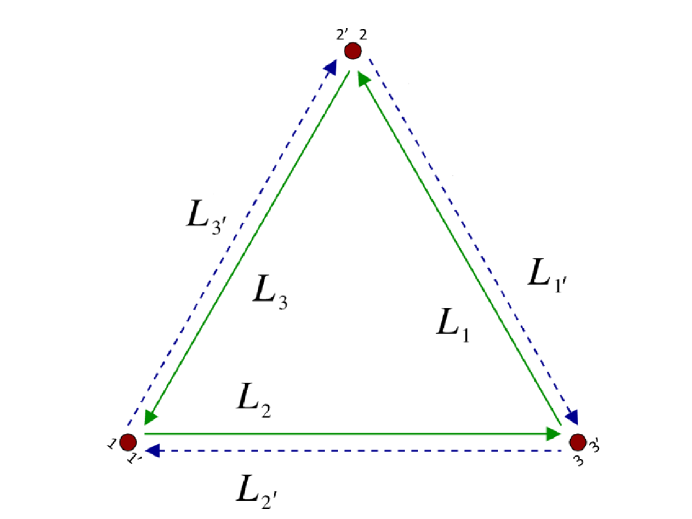
Figure 1: Schematic LISA configuration. The spacecraft are labeled $1$, $2$, and $3$, with their optical benches labeled with primed or unprimed indices depending on whether the received laser beam is propagating clockwise or counter-clockwise as seen from above the plane of the picture. The optical paths are denoted by $L_{i}$, $L_{i^{\prime}}$ where the index $i$ corresponds to the opposite spacecraft.

The eight heterodyne measurements performed onboard spacecraft # $1$ are presented in two groups, each including four data set from the specific optical bench where they are collected. The group of measurements from optical bench $1^{\prime}$ are represented by the following mathematical expressions (see Fig.(2))

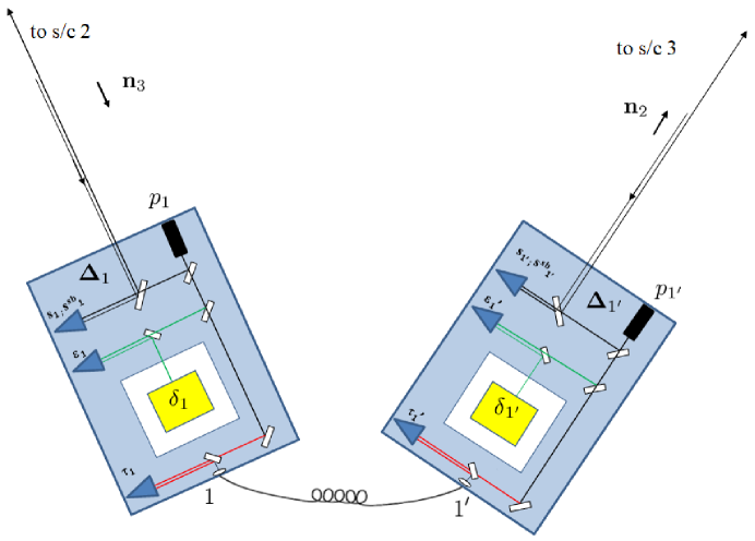
Figure 2: Schematic diagram of the proof-mass and optical bench assemblies for LISA spacecraft # 1. The left bench reads out a phase signal $s^{\rm c}_{1}$ from optical bench $2^{\prime}$ onboard spacecraft # $2$. The phase difference is measured by using the laser and the photo-detector on the left optical bench. The motion of the optical bench relative to the proof-mass is measured through internal metrology and results in the time series $\epsilon_{1}$. The relative phase fluctuations between the laser on the optical bench $1$ and the laser on the optical bench $1^{\prime}$ are instead captured by the measurements $\tau_{1}$ and $\tau_{1^{\prime}}$ respectively. Finally, the sideband-sideband phase differences, $s^{\rm sb}_{1}$ and $s^{\rm sb}_{1^{\prime}}$, capture the phase fluctuations of the USOs onboard spacecraft # $2$ and $3$ respectively relative to those of the USO onboard spacecraft $1$. These are the “essential ingredients” of the USO calibration algorithm.

$$s^{\rm c}_{1^{\prime}} = \left[H_{1^{\prime}}+{\cal D}_{2^{\prime}}p_{3}-p_{1^{\prime}}-2\pi\nu_{3}({\bf{n}}_{2^{\prime}}\cdot{\cal D}_{2^{\prime}}{\boldsymbol{\Delta}}_{3}+{\bf{n}}_{2}\cdot{\boldsymbol{\Delta}}_{1^{\prime}})+N_{1^{\prime}}^{\rm obt}\right]-a_{1^{\prime}}q_{1}+N_{1^{\prime}}^{\rm s}\ ,$$ (2)

$$s^{\rm sb}_{1^{\prime}} = \left[H_{1^{\prime}}+{\cal D}_{2^{\prime}}p_{3}-p_{1^{\prime}}+m_{3}{\cal D}_{2^{\prime}}q_{3}-m_{1^{\prime}}q_{1}-2\pi\nu_{3}({\bf{n}}_{2^{\prime}}\cdot{\cal D}_{2^{\prime}}{\boldsymbol{\Delta}}_{3}+{\bf{n}}_{2}\cdot{\boldsymbol{\Delta}}_{1^{\prime}})+N_{1^{\prime}}^{\rm obt.sb}\right]$$ (3)

$$- c_{1^{\prime}}q_{1}+N_{1^{\prime}}^{\rm sb}\ ,$$

$$\epsilon_{1^{\prime}} = \left[p_{1}-p_{1^{\prime}}+4\pi\nu_{1}({\bf{n}}_{2}\cdot{\boldsymbol{\delta}}_{1^{\prime}}-{\bf{n}}_{2}\cdot{\boldsymbol{\Delta}}_{1^{\prime}})+\mu_{1}\right]-b_{1^{\prime}}q_{1}+N_{1^{\prime}}^{\epsilon}\ ,$$ (4)

$$\tau_{1^{\prime}} = \left[p_{1}-p_{1^{\prime}}+\mu_{1}\right]-b_{1^{\prime}}q_{1}+N_{1^{\prime}}^{\tau}\ ,$$ (5)

while those from optical bench $1$ are equal to

$$s^{\rm c}_{1} = \left[H_{1}+{\cal D}_{3}p_{2^{\prime}}-p_{1}-2\pi\nu_{2^{\prime}}({\bf{n}}_{3}\cdot{\cal D}_{3}{\boldsymbol{\Delta}}_{2^{\prime}}+{\bf{n}}_{3^{\prime}}\cdot{\boldsymbol{\Delta}}_{1})+N_{1}^{\rm obt}\right]-a_{1}q_{1}+N_{1}^{\rm s}\ ,$$ (6)

$$s^{\rm sb}_{1} = \left[H_{1}+{\cal D}_{3}p_{2^{\prime}}-p_{1}+m_{2^{\prime}}{\cal D}_{3}q_{2}-m_{1}q_{1}-2\pi\nu_{2^{\prime}}({\bf{n}}_{3}\cdot{\cal D}_{3}{\boldsymbol{\Delta}}_{2^{\prime}}+{\bf{n}}_{3^{\prime}}\cdot{\boldsymbol{\Delta}}_{1})+N_{1}^{\rm obt.sb}\right]$$ (7)

$$- c_{1}q_{1}+N_{1}^{\rm sb}\ ,$$

$$\epsilon_{1} = \left[p_{1^{\prime}}-p_{1}+4\pi\nu_{1^{\prime}}({\bf{n}}_{3^{\prime}}\cdot{\boldsymbol{\delta}}_{1}-{\bf{n}}_{3^{\prime}}\cdot{\boldsymbol{\Delta}}_{1})+\mu_{1^{\prime}}\right]-b_{1}q_{1}+N_{1}^{\epsilon}\ ,$$ (8)

$$\tau_{1} = \left[p_{1^{\prime}}-p_{1}+\mu_{1^{\prime}}\right]-b_{1}q_{1}+N_{1}^{\tau}\ .$$ (9)

The observables $s^{\rm c},s^{\rm sb},\epsilon,\tau$ are the inter-spacecraft carrier-to-carrier and sideband-to-sideband one-way heterodyne measurements, the proof-mass-to-optical bench and the bench-to-bench metrology measurements respectively; the $a,b,c$ are the fractional frequency beat-note coefficients, i.e. the coefficients determined by the phasemeter Otto et al. (2012) that multiply the USO-referenced pilot-tone frequency so as to match the beat-note frequencies. The expressions of these coefficients are obtained from the corresponding ones given in Otto et al. (2012) by multiplying them by the appropriate $\theta$s. After performing such operation it is easy to show that they become equal to

$$a_{1^{\prime}} = \frac{\nu_{3}(1-{\dot{L}}_{2^{\prime}})-\nu_{1^{\prime}}}{f_{1}}\ \ ,$$ (10)

$$a_{1} = \frac{\nu_{2^{\prime}}(1-{\dot{L}}_{3})-\nu_{1}}{f_{1}}$$ (11)

$$b_{1^{\prime}} = \frac{\nu_{1}-\nu_{1^{\prime}}}{f_{1}}\ \ ,\ \ b_{1}=\frac{\nu_{1^{\prime}}-\nu_{1}}{f_{1}}=-b_{1^{\prime}}$$ (12)

$$c_{1^{\prime}} = \frac{(\nu_{3}+m_{3}f_{3})(1-{\dot{L}}_{2^{\prime}})-(\nu_{1^{\prime}}+m_{1^{\prime}}f_{1})}{f_{1}}\ \ ,$$ (13)

$$c_{1} = \frac{(\nu_{2^{\prime}}+m_{2^{\prime}}f_{2})(1-{\dot{L}}_{3})-(\nu_{1}+m_{1}f_{1})}{f_{1}}$$ (14)

In equations (2 - 9) the $H$-terms are the contributions to the measured phase fluctuations due to a possibly present transverse-traceless gravitational wave signal; the $p$- and $\nu$-terms represent the lasers’ phase noises and frequencies respectively; the $q$-terms are the phase noises due to the three USOs; the $N$-terms are shot-noise phase fluctuations at the photo-detectors; $L$-terms and $\dot{L}$-terms are the inter-spacecraft relative optical paths and their time-derivatives respectively; the $f$-terms are the USOs’ pilot-tones frequencies while the $m$-terms are integer numbers defining the modulation frequencies Otto et al. (2012); the ${\bf{n}}$-terms are unit vectors along the directions of propagation of the laser beams; the ${\boldsymbol{\Delta}}$-terms and ${\boldsymbol{\delta}}$-terms are vector random processes associated with the mechanical vibrations of the optical benches and proof-masses with respect to the local inertial reference frame respectively; the $\mu$-terms are phase fluctuations due to the optical fibers linking the two optical benches and they have been assumed to be independent of the direction of propagation of the optical beams within them (see Otto et al. (2012) for a clear discussion about this point); finally the ${\cal D}_{i}$, ${\cal D}_{j^{\prime}}$ are delay operators Tinto and Dhurandhar (2014).

Since the LISA array is both rotating and “flexing”, two delay operators do not commute in general Tinto and Dhurandhar (2014). For instance, with a laser noise equal to $30$ Hz/${\sqrt{\rm Hz}}$ in the mHz band Tinto and Dhurandhar (2014), the commutator of two delay operators applied to it results in residual fluctuations that are about an order of magnitude larger than those identified by the secondary noises. This is in fact the reason why the formulation of TDI for a static array is unable to suppress such a laser noise below the level identified by the secondary noises.

In the case of a LISA’s USO, however, its relative frequency fluctuations at optical frequency are significantly smaller than those of a laser. This means that the commutator of two delay operators applied to it results in relative frequency fluctuations significantly smaller than those due to the secondary noises. To be more quantitative, let us estimate the magnitude of the commutator of two delay operators applied to the phase fluctuations, $q(t)$, of a LISA USO. This is given by the following expression

$$[{\cal D}_{i},{\cal D}_{j}]q(t)=q(t-L_{i}(t)-L_{j}(t-L_{i}))-q(t-L_{j}(t)-L_{i}(t-L_{j}))\simeq[L_{i}{\dot{L}}_{j}-L_{j}{\dot{L}}_{i}]{\dot{q}}\ .$$ (15)

The right-hand-side of equation (15) implies the following order-of-magnitude estimate of the corresponding Fourier components of the relative frequency fluctuations (strain) amplitude, $\frac{|\widetilde{\Delta C_{q}}(f)|}{\nu_{0}}$, in a TDI combination

$$\frac{|\widetilde{\Delta C_{q}}(f)|}{\nu_{0}}\equiv\left(4\pi L{\dot{L}}\right)\left(\frac{af_{q}}{\nu_{0}}\right)\left(\frac{|{\widetilde{\dot{q}}}(f)|}{2\pi f_{q}}\right)\ f\ ,$$ (16)

where the $\widetilde{}$ symbol means “Fourier transform”, and $f$ is the Fourier frequency. By assuming a LISA USO characterized by a one-sided power spectral density of relative frequency fluctuations equal to $S_{y}(f)=6.7\times 10^{-27}f^{-1}\ {\rm Hz}^{-1}$ , a beat-note frequency $af_{q}=25\ {\rm MHz}$, a laser frequency $\nu_{0}=3\times 10^{14}$ Hz, a LISA arm-length (in seconds) $L=8.3$ sec. and an inter-spacecraft characteristic relative velocity $\dot{L}\simeq 3\times 10^{-8}$, we find the right-hand-side of equation (16) to be equal to $2.3\times 10^{-26}\ {\rm Hz}^{-1/2}$ at $f=1\ {\rm Hz}$ and smaller than this value at lower frequencies. Since this is more than five orders of magnitude smaller than the minimum of the strain sensitivity identified by the secondary noises in the TDI-1 combinations Tinto et al. (2002), we can treat two delay operators as commuting when they are applied to a LISA USO phase noise.

Before deriving the USO noise calibrating expressions, it is necessary to first remove the optical bench noises from the inter-spacecraft one-way measurements $s^{\rm c}$ Otto et al. (2012). This is done by using the differences $\epsilon-\tau$ from each optical bench as they contain the displacement of the optical bench relative to the proof-mass. Second, the laser phase-fluctuations with primed indices, $p_{i^{\prime}}$, can be expressed in terms of those with unprimed indices, $p_{i}$, by taking suitable linear combinations of the $s^{\rm c}_{i},\tau_{i},\tau_{j}$. This final operation results in the so called $\eta$-combinations, which depend only on the three unprimed laser phase fluctuations, $p_{i}$ Tinto and Dhurandhar (2014) and are not affected by the optical-bench noise.

As mentioned in section I, recent LISA Simulation Working Group activities have shown that the current algorithm Otto et al. (2012) to calibrate the USO noises out of the TDI-2 combinations is not performing as expected. To understand why, let us consider the one-way data measurements described by equations (2 - 9). Onboard each spacecraft there are two sets of them, one set per optical bench, with a total of $24$ data measurements after including those for the split-interferometry configuration and the sideband - sideband one-way inter-spacecraft Doppler data. From a simple counting argument we conclude that the number of observables is larger than the number of noises to be canceled. There are $6$ lasers, three USOs, and $12$ optical-bench noises for a total of $21$ random processes to be canceled by properly combining the $24$ data set. To solve this well-posed mathematical problem, the choice was made in Otto et al. (2012) to regard one of the USO noises to be equal to zero. This choice was based on the assumption that the USO noises enter in the heterodyne measurements as simple differences, and that therefore one of them could be set to zero. Unfortunately most of the measurements do not depend on the differences of the USO noises (see equations (2 - 9)). Those that do, such as the sideband-sideband measurements, depend on differences of USO noises measured at different times. This means that, even if all USO would ”glitch” equally, their differences would not cancel because of the light-time delays.

As it will be shown below, there exist TDI-2 combinations that cancel the laser phase fluctuations and from which it is in fact possible to calibrate out the USO noises to a sufficiently high-level of precision. This is done by properly time-shifting and linearly combining the $\eta$-observables and the one-way carrier-to-carrier and sideband-to-sideband measurements.

To minimize the length of the equations we will rely on, we will use expressions for the $\eta$-observables that display only the contributions from the laser and USO noises. Under this assumption, they assume the following forms

$$\eta_{1^{\prime}} = {\cal D}_{2^{\prime}}p_{3}-p_{1}+[-a_{1^{\prime}}+b_{1^{\prime}}]q_{1}\ ,$$ (17)

$$\eta_{1} = {\cal D}_{3}p_{2}-p_{1}-a_{1}q_{1}+b_{2}{\cal D}_{3}q_{2}\ ,$$ (18)

where the other four $\eta$-observables are obtained from the above expressions by permutation of the spacecraft indices.

III Clock-Noise Calibration from the TDI-2 Combinations

We describe the procedure for calibrating the USO noises out of the TDI-2 combinations by deriving the expressions for the unequal-arm Michelson interferometric combination $X_{1}$ and the Sagnac combination $\alpha_{1}$. The procedures described in this article can easily be extended to other TDI-2 combinations and for this reason we do not include them here.

III.1 The $X_{1}$ Combination

In terms of the $\eta$-observables, the TDI-2 unequal-arm Michelson combination, $X^{\rm q}_{1}$, is given by the following expression Tinto and Dhurandhar (2014)

$$X^{\rm q}_{1} = \left[{\cal D}_{3}{\cal D}_{3^{\prime}}{\cal D}_{2^{\prime}}{\cal D}_{2}-I\right]\left[(\eta_{1^{\prime}}+{\cal D}_{2^{\prime}}\eta_{3})+{\cal D}_{2^{\prime}}{\cal D}_{2}(\eta_{1}+{\cal D}_{3}\eta_{2^{\prime}})\right]$$ (19)

$$-\left[{\cal D}_{2^{\prime}}{\cal D}_{2}{\cal D}_{3}{\cal D}_{3^{\prime}}-I\right]\left[(\eta_{1}+{\cal D}_{3}\eta_{2^{\prime}})+{\cal D}_{3}{\cal D}_{3^{\prime}}(\eta_{1^{\prime}}+{\cal D}_{2^{\prime}}\eta_{3})\right]\ ,$$

where the label ^q emphasizes the USO-noise dependence. After substituting equations (17, 18) in equation (19) we have

$$X^{\rm q}_{1} = \left[{\cal D}_{3}{\cal D}_{3^{\prime}}{\cal D}_{2^{\prime}}{\cal D}_{2}-I\right]\left[b_{1}({\cal D}_{2^{\prime}}{\cal D}_{2}-I)q_{1}-a_{1}{\cal D}_{2^{\prime}}{\cal D}_{2}q_{1}-a_{1^{\prime}}q_{1}-a_{2^{\prime}}{\cal D}_{2^{\prime}}{\cal D}_{2}{\cal D}_{3}q_{2}-a_{3}{\cal D}_{2^{\prime}}q_{3}\right]$$ (20)

$$-\left[{\cal D}_{2^{\prime}}{\cal D}_{2}{\cal D}_{3}{\cal D}_{3^{\prime}}-I\right]\left[b_{1}{\cal D}_{3}{\cal D}_{3^{\prime}}({\cal D}_{2^{\prime}}{\cal D}_{2}-I)q_{1}-a_{1^{\prime}}{\cal D}_{3}{\cal D}_{3^{\prime}}q_{1}-a_{1}q_{1}-a_{2^{\prime}}{\cal D}_{3}q_{2}\right.$$

$$-\left.a_{3}{\cal D}_{3}{\cal D}_{3^{\prime}}{\cal D}_{2^{\prime}}q_{3}\right]\ .$$

Since the commutator of two delay operators applied to a LISA USO noise is, to a very good approximation, equal to zero, we can rewrite the above equation in the following form

$$X^{\rm q}_{1} \simeq \left[{\cal D}_{3}{\cal D}_{3^{\prime}}{\cal D}_{2^{\prime}}{\cal D}_{2}-I\right]\left[b_{1^{\prime}}(I-{\cal D}_{3}{\cal D}_{3^{\prime}})(I-{\cal D}_{2^{\prime}}{\cal D}_{2})q_{1}+a_{1}(I-{\cal D}_{2^{\prime}}{\cal D}_{2})q_{1}\right.$$ (21)

$$- \left.a_{1^{\prime}}(I-{\cal D}_{3}{\cal D}_{3^{\prime}})q_{1}+a_{2^{\prime}}{\cal D}_{3}(I-{\cal D}_{2^{\prime}}{\cal D}_{2})q_{2}-a_{3}{\cal D}_{2^{\prime}}(I-{\cal D}_{3}{\cal D}_{3^{\prime}})q_{3}\right]\ ,$$

where we have factored out the delay-operator $[{\cal D}_{3}{\cal D}_{3^{\prime}}{\cal D}_{2^{\prime}}{\cal D}_{2}-I]$.

It is important to note that the $q$-terms in the square-bracket in equation (21) can easily be related to those in equation (9) of Tinto et al. (2002), which are for the TDI-1 combination $X$ of a static LISA. This means that the expressions calibrating the USO noises out of the TDI-2 combination $X_{1}$ can be derived by using the approach of Tinto et al. (2002) for the static-array unequal-arm Michelson combination $X$.

Following Armstrong, Estabrook and Tinto Tinto et al. (2002), let us introduce the following linear combinations of the carrier-to-carrier and sideband-to-sideband one-way heterodyne measurements

$$r_{1^{\prime}} \equiv \frac{s^{\rm c}_{1^{\prime}}-s^{\rm sb}_{1^{\prime}}}{m_{3}f_{3}}\ ,$$ (22)

$$r_{1} \equiv \frac{s^{\rm c}_{1}-s^{\rm sb}_{1}}{m_{2^{\prime}}f_{2}}\ .$$ (23)

Note that the above observables differ from those given in Tinto et al. (2002) by the presence of the modulation frequency integers $m_{2^{\prime}}$ and $m_{3}$. After substituting in equations (22, 23) the expressions for the one-way heterodyne measurements, $s^{\rm c}$, $s^{\rm sb}$ (equations (2, 3, 6, 7)) after some algebra it is possible to obtain the following expressions for $r_{1^{\prime}}\ ,r_{1}$

$$r_{1^{\prime}} = \frac{(1-{\dot{L}}_{2^{\prime}})}{f_{1}}q_{1}-\frac{{\cal D}_{2^{\prime}}q_{3}}{f_{3}}\ ,$$ (24)

$$r_{1} = \frac{(1-{\dot{L}}_{3})}{f_{1}}q_{1}-\frac{{\cal D}_{3}q_{2}}{f_{2}}\ .$$ (25)

By neglecting terms proportional to $\dot{L}$, equations (25) can be rewritten to sufficient precision in the following form

$$r_{1^{\prime}} = \frac{q_{1}}{f_{1}}-\frac{{\cal D}_{2^{\prime}}q_{3}}{f_{3}}\ ,$$ (26)

$$r_{1} = \frac{q_{1}}{f_{1}}-\frac{{\cal D}_{3}q_{2}}{f_{2}}\ ,$$ (27)

with the remaining expressions obtained by cyclic permutations of the spacecraft indices. Note that the dependence on the $m$-integers has dropped-out from the $r$-combinations (equations 26, 27), which are essentially equal to the corresponding ones in Tinto et al. (2002) after modifying them to account for the inequality of the delays experienced by laser beams propagating along opposite directions (Sagnac effect).

Note also that, since there are only three USO noises $q_{i}$, there exist relationships relating the six calibration data $(r_{i},r_{i^{\prime}})\ ,\ i=1,2,3\ ,\ i^{\prime}=1^{\prime},2^{\prime},3^{\prime}$. Because the mathematical structure of the $r$-observables (equations (26, 27)) is equal to that of the one-way measurements in which the random processes $q_{i}/f_{i}$ play the same role as the laser phase noises, we infer that such relationships belong to the TDI-space.

By using the equations (26, 27) and following Tinto et al. (2002) it is easy to derive the following identities

$$\left[I-{\cal D}_{2^{\prime}}{\cal D}_{2}\right]q_{1} = f_{1}\ (r_{1^{\prime}}+{\cal D}_{2^{\prime}}r_{3})\ ,$$ (28)

$$\left[I-{\cal D}_{3}{\cal D}_{3^{\prime}}\right]q_{1} = f_{1}\ (r_{1}+{\cal D}_{3}r_{2^{\prime}})\ ,$$ (29)

$${\cal D}_{3}\left[I-{\cal D}_{2^{\prime}}{\cal D}_{2}\right]q_{2} = f_{2}\ [r_{1^{\prime}}-(I-{\cal D}_{2^{\prime}}{\cal D}_{2})r_{1}+{\cal D}_{2^{\prime}}r_{3}]\ ,$$ (30)

$${\cal D}_{2^{\prime}}\left[I-{\cal D}_{3}{\cal D}_{3^{\prime}}\right]q_{3} = f_{3}\ [r_{1}-(I-{\cal D}_{3}{\cal D}_{3^{\prime}})r_{1^{\prime}}+{\cal D}_{3}r_{2^{\prime}}]\ .$$ (31)

By first applying the delay operator $[{\cal D}_{3}{\cal D}_{3^{\prime}}{\cal D}_{2^{\prime}}{\cal D}_{2}-I]$ to equations (28 - 31) and substituting the resulting expressions into equation (21) we finally find the following USO-corrected $X_{1}$ combination

$$X_{1} \equiv X^{\rm q}_{1}-\left[{\cal D}_{3}{\cal D}_{3^{\prime}}{\cal D}_{2^{\prime}}{\cal D}_{2}-I\right]\Bigl{[}b_{1^{\prime}}\ \frac{f_{1}}{2}\ [(I-{\cal D}_{3}{\cal D}_{3^{\prime}})\ (r_{1^{\prime}}+{\cal D}_{2^{\prime}}r_{3})+(I-{\cal D}_{2^{\prime}}{\cal D}_{2})\ (r_{1}+{\cal D}_{3}r_{2^{\prime}})]\Bigr{.}$$ (32)

$$+\Bigl{.}a_{1}\ f_{1}\ [r_{1^{\prime}}+{\cal D}_{2^{\prime}}r_{3}]-a_{1^{\prime}}\ f_{1}\ [r_{1}+{\cal D}_{3}r_{2^{\prime}}]+a_{2^{\prime}}\ f_{2}\ [r_{1^{\prime}}-(I-{\cal D}_{2^{\prime}}{\cal D}_{2})r_{1}+{\cal D}_{2^{\prime}}r_{3}]\Bigr{.}$$

$$-\Bigl{.}a_{3}\ f_{3}\ [r_{1}-(I-{\cal D}_{3}{\cal D}_{3^{\prime}})r_{1^{\prime}}+{\cal D}_{3}r_{2^{\prime}}]\Bigr{]}$$

Since the unequal-arm Michelson interferometric response $X_{1}$ is antisymmetric with respect to permutations of the indices (2,3’), (3,2’), (1,1’), the corresponding combinations used for calibrating out the USO noise from $X^{\rm q}_{1}$ have been antisymmetrized by relying on the equations (28 - 31) and taking advantage of the commutativity of two delay operators applied to a LISA USO noise. The other two unequal-arm Michelson responses, $X_{2}$ and $X_{3}$, follow from equation (32) after performing a cyclic permutation of the spacecraft indices.

III.2 The $\alpha_{1}$ Combination

In terms of the $\eta$-observables, the TDI-2 Sagnac combination, $\alpha^{\rm q}_{1}$, is given by the following expression Tinto and Dhurandhar (2014)

$$\alpha^{\rm q}_{1}=[{\cal D}_{3}{\cal D}_{1}{\cal D}_{2}-I]\,[\eta_{1^{\prime}}+{\cal D}_{2^{\prime}}\eta_{3^{\prime}}+{\cal D}_{2^{\prime}}{\cal D}_{1^{\prime}}\eta_{2^{\prime}}]-[{\cal D}_{2^{\prime}}{\cal D}_{1^{\prime}}{\cal D}_{3^{\prime}}-I]\,[\eta_{1}+{\cal D}_{3}\eta_{2}+{\cal D}_{3}{\cal D}_{1}\eta_{3}]\ .$$ (33)

After substituting equations (17, 18) in equation (33) we have

$$\alpha^{\rm q}_{1} = [{\cal D}_{3}{\cal D}_{1}{\cal D}_{2}-I]\,[(b_{1^{\prime}}-a_{1^{\prime}})\ q_{1}\ +\ {\cal D}_{2^{\prime}}{\cal D}_{1^{\prime}}(b_{2^{\prime}}-a_{2^{\prime}})\ q_{2}\ +\ {\cal D}_{2^{\prime}}(b_{3^{\prime}}-a_{3^{\prime}})q_{3}]$$ (34)

$$-[{\cal D}_{2^{\prime}}{\cal D}_{1^{\prime}}{\cal D}_{3^{\prime}}-I]\,[(-a_{1}+b_{1}{\cal D}_{3}{\cal D}_{1}{\cal D}_{2})\ q_{1}\ +\ (-a_{2}+b_{2}){\cal D}_{3}q_{2}$$

$$\ +\ (-a_{3}+b_{3})\ {\cal D}_{3}{\cal D}_{1}q_{3}]\ .$$

Following a reasoning similar to the one made earlier to evaluate the commutator of two delay-operators applied to a USO noise, it is easy to show that also $({\cal D}_{3^{\prime}}{\cal D}_{2^{\prime}}{\cal D}_{1^{\prime}}-{\cal D}_{3}{\cal D}_{2}{\cal D}_{1})q\simeq 0$, where the $\simeq 0$ means: “it results in relative frequency fluctuations (strain) significantly smaller than those identified by the acceleration and optical-path noises”. Equation (34) can therefore be rewritten in the following form

$$\alpha^{\rm q}_{1} = [{\cal D}_{3}{\cal D}_{1}{\cal D}_{2}-I]\,\Bigl{[}(a_{1}-a_{1^{\prime}})\ q_{1}\ +\ b_{1^{\prime}}(I+{\cal D}_{3}{\cal D}_{1}{\cal D}_{2})q_{1}\ +\ [{\cal D}_{2^{\prime}}{\cal D}_{1^{\prime}}(b_{2^{\prime}}-a_{2^{\prime}})\Bigr{.}$$ (35)

$$\Bigl{.}\ +\ (a_{2}-b_{2}){\cal D}_{3}]\ q_{2}\ +\ [{\cal D}_{3}{\cal D}_{1}(a_{3}-b_{3})\ +\ (b_{3^{\prime}}-a_{3^{\prime}}){\cal D}_{2^{\prime}}]\ q_{3}\Bigr{]}\ ,$$

after having factored out the delay operator $[{\cal D}_{3}{\cal D}_{1}{\cal D}_{2}-I]$.

Since the expression inside the large square-brackets is (apart from the primed-delays due to the Sagnac effect) the same as that of the TDI-1 combination $\alpha$ given in Tinto et al. (2002), and because it was shown there that it is impossible to exactly calibrate out of $\alpha$ the USO noise using the $r$-combinations Hellings (2001), it follows that also for $\alpha_{1}$ it is impossible to exactly calibrate out the USO noise. As shown in Tinto et al. (2002), however, we can rewrite the USO phase noises in terms of some of the $r$-data and only the USO phase noise $q_{1}$ by using the following additional identities

$${\cal D}_{3}{\cal D}_{1}{\cal D}_{2}q_{1} = q_{1}-f_{1}\ [{\cal D}_{3}{\cal D}_{1}r_{3}+{\cal D}_{3}r_{2}+r_{1}]\ ,$$ (36)

$${\cal D}_{2^{\prime}}{\cal D}_{1^{\prime}}q_{2} = \frac{f_{2}}{f_{1}}\ q_{1}-f_{2}\ [r_{1^{\prime}}+{\cal D}_{2^{\prime}}r_{3^{\prime}}]\ \ ,$$ (37)

$${\cal D}_{3}{\cal D}_{1}q_{3} = \frac{f_{3}}{f_{1}}\ q_{1}-f_{3}\ [r_{1}+{\cal D}_{3}r_{2}]\ \ ,$$ (38)

$${\cal D}_{3}q_{2} = \frac{f_{2}}{f_{1}}\ q_{1}-f_{2}\ r_{1}\ \ ,$$ (39)

$${\cal D}_{2^{\prime}}q_{3} = \frac{f_{3}}{f_{1}}\ q_{1}-f_{3}\ r_{1^{\prime}}\ .$$ (40)

The USO noise terms involving the $q_{i}$ in equation (35) then become

$$\left[(a_{1}-a_{1^{\prime}}+2b_{1^{\prime}})\ f_{1}\ +\ (a_{2}-a_{2^{\prime}}+2b_{2^{\prime}})\ f_{2}\ +\ (a_{3}-a_{3^{\prime}}+2b_{3^{\prime}})\ f_{3}\right]\ \frac{q_{1}}{f_{1}}$$ (41)

$$-f_{1}\ b_{1^{\prime}}\ [r_{1}+{\cal D}_{3}r_{2}+{\cal D}_{3}{\cal D}_{1}r_{3}]-f_{2}\ [b_{2^{\prime}}+a_{2}]\ r_{1}-f_{3}\ [b_{3^{\prime}}-a_{3^{\prime}}]\ r_{1^{\prime}}$$

$$-f_{2}\ [b_{2^{\prime}}-a_{2^{\prime}}]\ [r_{1^{\prime}}+{\cal D}_{2^{\prime}}r_{3^{\prime}}]-f_{3}\ [b_{3^{\prime}}+a_{3}]\ [r_{1}+{\cal D}_{3}r_{2}]\ .$$

If we now take into account the expressions for the $a$- and $b$-coefficients, the first term in equation (41) can be reduced to the following form

$$\left[(\nu_{2}-\nu_{3^{\prime}}){\dot{L}_{1}}+(\nu_{3}-\nu_{1^{\prime}}){\dot{L}_{2}}+(\nu_{1}-\nu_{2^{\prime}}){\dot{L}_{3}}\right]\ \frac{q_{1}}{f_{1}}\ ,$$ (42)

This corresponds to relative frequency fluctuations (or strain noise) of the order of about $10^{-27}$ under the assumptions of having laser frequency offsets of a few hundred megahertz, a laser center frequency equal to $3\times 10^{14}$ Hz, Doppler term $\dot{L}_{i}$ equal to about $3\times 10^{-8}$, and a USO frequency stability of about $10^{-13}$. Thus we can ignore it and, after some algebra, define the laser-noise-free and USO-noise-free reduced data $\alpha_{1}$ to be

$$\alpha_{1} \equiv \alpha^{\rm q}_{1}+[{\cal D}_{3}{\cal D}_{1}{\cal D}_{2}-I]\,\Bigl{[}\frac{1}{2}\ f_{1}\ b_{1^{\prime}}[(r_{1}+{\cal D}_{3}r_{2}+{\cal D}_{3}{\cal D}_{1}r_{3})+(r_{1^{\prime}}+{\cal D}_{2^{\prime}}r_{3^{\prime}}+{\cal D}_{2^{\prime}}{\cal D}_{1^{\prime}}r_{2^{\prime}})]\Bigr{.}$$ (43)

$$+\Bigl{.}f_{2}(b_{2^{\prime}}+a_{2})r_{1}\ +\ f_{3}(b_{3^{\prime}}-a_{3^{\prime}})r_{1^{\prime}}\ +\ f_{2}(b_{2^{\prime}}-a_{2^{\prime}})(r_{1^{\prime}}+{\cal D}_{2^{\prime}}r_{3^{\prime}})\Bigr{.}$$

$$+\Bigl{.}f_{3}(b_{3^{\prime}}+a_{3})(r_{1}+{\cal D}_{3}r_{2})\Bigr{]}$$

Like $X_{1}$, also $\alpha_{1}$ should be antisymmetric with respect to permutation of the indices (2,3’), (3,2’), (1,1’). The combinations in equation (41) used for calibrating out the USO noise from $\alpha^{\rm q}_{1}$ have therefore, in equation (43), been antisymmetrized. The remaining two TDI-2 Sagnac responses, denoted $\alpha_{2}$ and $\alpha_{3}$, follow from equation (43) after performing cyclic permutation of the spacecraft indices.

IV Conclusions

This article addresses the problem of calibrating the onboard clock phase fluctuations out of the second-generation TDI combinations. We have focused our analysis on deriving calibrating expressions for the unequal-arm Michelson combination $X_{1}$ and the Sagnac combination $\alpha_{1}$ as similar procedures can be extended to all other second-generation TDI combinations. Our approach relies on the key observation that the commutator of two delay operators applied to a LISA USO noise results in relative frequency fluctuations that are significantly smaller than those of the secondary noises and can therefore be neglected.

Although the sideband-sideband technique suppresses the LISA’s USO noises to levels significantly smaller than that identified by the secondary noises, it does not cancel them exactly. This might result in a sensitivity limitation for more ambitious missions characterized by higher sensitivities and/or significantly larger beat-notes Crowder and Cornish (2005); Gang and Wei-Tou (2013). This is because the calibrating algorithm presented here might not sufficiently suppress the USO noises in their TDI-2 combinations. The use of optical frequency-comb, on the other hand, provides a solution in these cases by generating the microwave signal frequency coherent to the frequency of the onboard laser. This is because the optical frequency-comb technique exactly cancels the microwave signal phase fluctuations by using modified TDI-2 combinations and it does not require modulated beams.

In addition, use of an optical frequency comb may result in a simplification of the LISA’s onboard interferometry system Tinto and Yu (2015) because (i) generation of modulated beams and additional heterodyne measurements involving clock microwave sidebands will no longer be needed, and (ii) the entire onboard USO subsystem can be replaced with the microwave signal referenced to the onboard laser. This may result in a reduced system complexity and probability of subsystem failure. Recent progress in the realization of a space-qualified optical frequency comb indicates that such a capability will be available well before LISA’s launching date Giunta et al. (2016).

References

- Abbott and et al (2016a) B. P. Abbott and et al (LIGO Scientific Collaboration and Virgo Collaboration), Phys. Rev. Lett. 116, 061102 (2016a), URL https://link.aps.org/doi/10.1103/PhysRevLett.116.061102.
- Abbott and et al (2016b) B. P. Abbott and et al (LIGO Scientific Collaboration and Virgo Collaboration), Phys. Rev. Lett. 116, 241103 (2016b), URL https://link.aps.org/doi/10.1103/PhysRevLett.116.241103.
- Abbott and et al (2017a) B. P. Abbott and et al (LIGO Scientific and Virgo Collaboration), Phys. Rev. Lett. 118, 221101 (2017a), URL https://link.aps.org/doi/10.1103/PhysRevLett.118.221101.
- Abbott and et al (2017b) B. P. Abbott and et al (LIGO Scientific Collaboration and Virgo Collaboration), Phys. Rev. Lett. 119, 141101 (2017b), URL https://link.aps.org/doi/10.1103/PhysRevLett.119.141101.
- Abbott and et al (2017c) B. P. Abbott and et al (LIGO Scientific Collaboration and Virgo Collaboration), Phys. Rev. Lett. 119, 161101 (2017c), URL https://link.aps.org/doi/10.1103/PhysRevLett.119.161101.
- Amaro-Seoane and et al (2017) P. Amaro-Seoane and et al, ArXiv e-prints: https://arxiv.org/abs/1702.00786 (2017), eprint 1702.00786.
- Tinto et al. (2002) M. Tinto, F. B. Estabrook, and J. W. Armstrong, Phys. Rev. D 65, 082003 (2002), URL https://link.aps.org/doi/10.1103/PhysRevD.65.082003.
- Hellings et al. (1996) R. Hellings, G. Giampieri, L. Maleki, M. Tinto, K. Danzmann, J. Hough, and D. Robertson, Optics Communications 124, 313 (1996), ISSN 0030-4018, URL http://www.sciencedirect.com/science/article/pii/0030401895006842.
- Hellings (2001) R. W. Hellings, Phys. Rev. D 64, 022002 (2001), URL https://link.aps.org/doi/10.1103/PhysRevD.64.022002.
- Tinto and Yu (2015) M. Tinto and N. Yu, Phys. Rev. D 92, 042002 (2015), URL https://link.aps.org/doi/10.1103/PhysRevD.92.042002.
- Hall (2006) J. L. Hall, Rev. Mod. Phys. 78, 1279 (2006), URL https://link.aps.org/doi/10.1103/RevModPhys.78.1279.
- Hänsch (2006) T. W. Hänsch, Rev. Mod. Phys. 78, 1297 (2006), URL https://link.aps.org/doi/10.1103/RevModPhys.78.1297.
- Giunta et al. (2016) M. Giunta, M. Lezius, C. Deutsch, T. Wilken, T. W. Hänsch, A. Kohfeldt, A. Wicht, V. Schkolnik, M. Krutzik, H. Duncker, et al., in Conference on Lasers and Electro-Optics (Optical Society of America, 2016), p. STh4H.5, URL http://www.osapublishing.org/abstract.cfm?URI=CLEO_SI-2016-STh4H.5.
- Otto et al. (2012) M. Otto, G. Heinzel, and K. Danzmann, Classical and Quantum Gravity 29, 205003 (2012), URL http://stacks.iop.org/0264-9381/29/i=20/a=205003.
- Tinto and Dhurandhar (2014) M. Tinto and S. V. Dhurandhar, Living Reviews in Relativity 17, 6 (2014), ISSN 1433-8351, URL https://doi.org/10.12942/lrr-2014-6.
- Barnes et al. (1971) J. A. Barnes, A. R. Chi, L. S. Cutler, D. J. Healey, D. B. Leeson, T. E. McGunigal, J. A. Mullen, W. L. Smith, R. L. Sydnor, R. F. C. Vessot, et al., IEEE Transactions on Instrumentation and Measurement IM-20, 105 (1971), ISSN 0018-9456.
- Crowder and Cornish (2005) J. Crowder and N. J. Cornish, Phys. Rev. D 72, 083005 (2005), URL https://link.aps.org/doi/10.1103/PhysRevD.72.083005.
- Gang and Wei-Tou (2013) W. Gang and N. Wei-Tou, Chinese Physics B 22, 049501 (2013), URL http://stacks.iop.org/1674-1056/22/i=4/a=049501.