Leveraging Well-Conditioned Bases: Streaming and
Distributed Summaries in Minkowski $p$-Norms

Abstract

Work on approximate linear algebra has led to efficient distributed and streaming algorithms for problems such as approximate matrix multiplication, low rank approximation, and regression, primarily for the Euclidean norm $\ell_{2}$. We study other $\ell_{p}$ norms, which are more robust for $p<2$, and can be used to find outliers for $p>2$. Unlike previous algorithms for such norms, we give algorithms that are (1) deterministic, (2) work simultaneously for every $p\geq 1$, including $p=\infty$, and (3) can be implemented in both distributed and streaming environments. We apply our results to $\ell_{p}$-regression, entrywise $\ell_{1}$-low rank approximation, and approximate matrix multiplication.

*EndProcedure

1 Introduction

Analyzing high dimensional, high volume data can be time-consuming and resource intensive. Core data analysis, such as robust instances of regression, involve convex optimization tasks over large matrices, and do not naturally distribute or parallelize. In response to this, approximation algorithms have been proposed which follow a “sketch and solve” paradigm: produce a reduced size representation of the data, and solve a version of the problem on this summary (Woodruff, 2014). It is then argued that the solution on the reduced data provides an approximation to the original problem on the original data. This paradigm is particularly attractive when the summarization can be computed efficiently on partial views of the full data—for example, when it can be computed incrementally as the data arrives (streaming model) or assembled from summarizations of disjoint partitions of the data (distributed model) (Woodruff, 2014; Agarwal et al., 2012; Feldman et al., 2006). This template has been instantiated for a number of fundamental tasks in high dimensional linear algebra such as matrix multiplication, low rank approximation, and regression.

Our understanding is well-established in the common case of the Euclidean norm, i.e., when distances are measured under the Minkowski $p$-norm for $p=2$. Here, it suffices to choose a sketching matrix independent of the data—where each entry is i.i.d. Gaussian, Rademacher, or more efficient variants of these. For other $p$ values, less is known, but these are often needed to handle limitations of the $2$-norm. For instance, $p=1$ is widely used as it is extremely robust with respect to the presence of outliers while $p>2$ can be used to detect outlying observations.

We continue the study of algorithms for $\ell_{p}$ norms on streaming and distributed data. A particular novelty of our results is that unlike previous distributed and streaming algorithms, they can all be implemented deterministically, i.e., our algorithms make no random choices. While in a number of settings randomized algorithms are highly beneficial, leading to massive computational savings, there are other applications which require extremely high reliability, for which one needs to obtain guaranteed performance across a large number of inputs. If one were to use a randomized algorithm, then it would need vanishingly small error probability; however, many celebrated algorithms in numerical linear algebra succeed with only constant probability. Another limitation of randomized algorithms was shown in (Hardt & Woodruff, 2013): if the input to a randomized sketch depends on the output of a preceding algorithm using the same sketch, then the randomized sketch can give an arbitrarily bad answer. Hence, such methods cannot handle adaptively chosen inputs. Thus, while randomized algorithms certainly have their place, the issues of high reliability and adaptivity motivate the development of deterministic methods for a number of other settings, for which algorithms are scarce.

Our techniques can be viewed as a conceptual generalization of Liberty’s Frequent Directions (in the $2$-norm) (Liberty, 2013), which progressively computes an SVD on subsequent blocks of the input. This line of work (Liberty, 2013; Ghashami & Phillips, 2014; Ghashami et al., 2016, 2016) is the notable exception in numerical linear algebra, as it provides deterministic methods, although all such methods are specific to the 2-norm. Our core algorithm is similar in nature, but we require a very different technical analysis to argue that the basis transformation computed preserves the shape in the target $p$-norm.

Our main application is to show how high dimensional regression and low rank approximation problems can be solved approximately and deterministically in the sketch and solve paradigm. The core of the summary is to find rows of the original matrix which have high leverage scores. That is, they contain a lot of information about the shape of the data. In the Euclidean norm, leverage scores correspond directly to row norms of an orthonormal basis. This is less straightforward for other $\ell_{p}$ norms, where the scores correspond to the row norms of so-called $\ell_{p}$-well-conditioned bases. Moreover, while leverage scores are often used for sampling in randomized algorithms, we use them here in the context of fully deterministic algorithms.

We show how a superset of rows with high leverage scores can be found for arbitrary $\ell_{p}$ norms, based on only local information. This leads to efficient algorithms which identify rows with high (local) leverage scores within subsets of the data, and proceed hierarchically to collect a sufficient set of rows. These rows then allow us to solve regression problems: essentially, we solve the regression problem corresponding to just the retained input rows. We apply this technique to $\ell_{p}$-regression and entrywise $\ell_{p}$-low rank approximation. In particular, we use it to solve the $\ell_{\infty}$-regression problem with additive error in a stream. Note that the $\ell_{\infty}$ problem reduces to finding a ball of minimum radius which covers the data, and global solutions are slow due to the need to solve a linear program. Instead, we show that only a subset of the data needs to be retained in the streaming model to compute accurate approximations. Given the relationship between the streaming model and the distributed model that we later define, this could be seen in the context of having data stored over multiple machines who could send ‘important’ rows of their data to a central coordinator in order to compute the approximation.

Summary of Results. All our algorithms are deterministic polynomial time, and use significantly sublinear memory or communication in streaming and distributed models, respectively. We consider tall and thin $n\times d$ matrices $A$ for overconstrained regression so one should think of $n\gg d$. We implement both deterministic and randomized variants of our algorithms.
Section 3 presents an algorithm which returns rows of high ‘importance’ in a data matrix with additive error. This follows by storing a polynomial number (in $d$) of rows and using these to compute a well-conditioned basis. The key insight here is that rows of high norm in the full well-conditioned basis cannot have their norm decrease too much in a well-conditioned basis associated with a subblock; in fact they remain large up to a multiplicative poly$(d)$ factor.
Section 4 gives a method for computing a so-called $\ell_{p}$-subspace embedding of a data matrix in polynomial time. The space is $n^{\gamma}$ to obtain $d^{O(1/\gamma)}$ distortion, for $\gamma\in(0,1)$ a small constant. This result is then applied to $\ell_{p}$-regression which is shown to have a poly$(d)$ approximation factor with the same amount of space.
Section 5 describes a deterministic algorithm which gives a poly$(k)$-approximation to the optimal low rank approximation problem in entrywise $\ell_{1}$-norm. It runs in polynomial time for constant $k$. This method builds on prior work by derandomizing a subroutine from (Song et al., 2017).
Section 6 describes an algorithm for computing an additive-error solution to the $\ell_{\infty}$-regression problem, and shows a corresponding lower bound, showing that relative error solutions in this norm are not possible in sublinear space, even for randomized algorithms.
Section 7 concludes with an empirical evaluation. More experiments, intermediate results, and formal proofs can be found in the Supplementary Material, as can results on approximate matrix multiplication.

Comparison to Related Work. There is a rich literature on algorithms for numerical linear algebra in general $p$-norms; most of which are randomized with the notable exception of Frequent Directions. The key contributions of our work for each of the problems considered and its relation to prior work is as follows:

Finding high leverage rows: our algorithm is a single pass streaming algorithm and uses small space. We show that the global property of $\ell_{p}$-leverage scores can be understood by considering only local statistics. Frequent Directions is the only comparable result to ours and outputs a summary of the rows only in the $\ell_{2}$-norm. However, our method covers all $p\geq 1$. Theorem 3.3 is the key result and is later used to prove Theorem 6.1 and approximate the $\ell_{\infty}$-regression problem.

Subspace embedding, regression and $\ell_{1}$ low-rank approximation: various approaches using row-sampling (Cohen & Peng, 2015; Dasgupta et al., 2008), and data oblivious methods such as low-distortion embeddings can solve regression in time proportional to the sparsity of the input matrix (Clarkson et al., 2013; Meng & Mahoney, 2013; Song et al., 2017; Woodruff & Zhang, 2013). However, despite the attractive running times and error guarantees of these works, they are all randomized and do not necessarily translate well to the streaming model of computation. Our contribution here is a fully deterministic algorithm that works for all $p\geq 1$ in both streaming and distributed models. Randomized methods for $\ell_{1}$ low-rank approximation have also been developed in (Song et al., 2017) and our result exploits a derandomized subroutine from this work to obtain a deterministic result which applies in both models.

2 Preliminaries and Notation

We consider computing $\ell_{p}$-leverage scores of a matrix, low-rank approximation, regression, and matrix multiplication. We assume the input is a matrix $A\in\mathbb{R}^{n\times d}$ and $n\gg d$ so $\operatorname{rank}(A)\leq d$ and the regression problems are overconstrained. Without loss of generality we may assume that the columns of the input matrix are linearly independent so that $\operatorname{rank}(A)=d$. Throughout this paper we rely heavily on the notion of a well-conditioned basis for the column space of an input matrix, in the context of the entrywise $p$-norm which is $\|A\|_{p}=(\sum_{i,j}|A_{ij}|^{p})^{1/p}$.

Definition 2.1 (Well-conditioned basis).

Let $A\in\mathbb{R}^{n\times d}$ have rank $d$. For $p\in[1,\infty)$ let $q=\frac{p}{p-1}$ be its dual norm. An $n\times d$ matrix $U$ is an $(\alpha,\beta,p)$-well-conditioned basis for $A$ if the column span of $U$ is equal to that of $A$, $\|U\|_{p}\leq\alpha$, for all $z\in\mathbb{R}^{d},\|z\|_{q}\leq\beta\|Uz\|_{p}$ , and $\alpha,\beta,d^{O(1)}$ are independent of $n$ (Dasgupta et al., 2008).

We focus on the cases $p<2$ and $p>2$ because the deterministic $p=2$ case is relatively straightforward. Indeed, for $p=2$, $A^{T}A$ can be maintained incrementally as rows are added, allowing $x^{T}A^{T}Ax$ to be computed for any vector $x$. So it is possible to find an exact $\ell_{2}$ subspace embedding using $O(d^{2})$ space in a stream and $O(nd^{\omega-1})$ time ($\omega$ is the matrix multiplication constant). We adopt the convention that when $p=1$ we take $q=\infty$.

Theorem 2.2 ((Dasgupta et al., 2008)).

Let $A$ be an $n\times d$ matrix of rank $d$, let $p\in[1,\infty)$ and let $q$ be its dual norm. There exists an $(\alpha,\beta,p)$-well-conditioned basis $U$ for the column space of $A$ such that:

1. if $p<2$ then $\alpha=d^{\frac{1}{p}+\frac{1}{2}}$ and $\beta=1$,

2. if $p=2$ then $\alpha=\sqrt{d}$ and $\beta=1$, and

3. if $p>2$ then $\alpha=d^{\frac{1}{p}+\frac{1}{2}}$ and $\beta=d^{\frac{1}{p}-\frac{1}{2}}$.

Moreover, $U$ can be computed in deterministic time $O(nd^{2}+nd^{5}\log n)$ for $p\neq 2$ and $O(nd^{2})$ if $p=2$.

We freely use the fact that a well-conditioned basis $U=AR$ can be efficiently computed for the given data matrix $A$. Details for the computation can be found in (Dasgupta et al., 2008) but this is done by computing a change of basis $R$ such that $U=AR$ is well-conditioned. Similarly, as $R$ can be inverted we have the relation that $UR^{-1}=A$. Both methods are used so we adopt the convention that $U=AR$ when writing a well-conditioned basis in terms of the input and $US=A$ for the input in terms of the basis.

2.1 Computation Models

Our algorithms operate under the streaming and distributed models of computation. In both settings an algorithm receives as input a matrix $A\in\mathbb{R}^{n\times d}$. For a problem P, the algorithm must keep a subset of the rows of $A$ and, upon reading the full input, may use a black-box solver to compute an approximate solution to P with only the subset of rows stored. In both models we measure the summary size (storage), the update time which is the time taken to find the local summary, and the query time which is the time taken to compute an approximation to P using the summary.

The Streaming Model: The rows of $A$ are given to the (centralized) algorithm one-by-one. Let $b$ be the maximum number of rows that can be stored under the constraint that $b$ is sublinear in $n$. The stored subset is used to compute local statistics which determine those rows to be kept or discarded from the stored set. Further rows are then appended and the process is repeated until the full matrix has been read. An approximation to the problem is then computed by solving P on the reduced subset of rows.

The Distributed Summary Model: Given a small constant $\gamma\in(0,1)$, the input in the form of matrix $A\in\mathbb{R}^{n\times d}$ is partitioned into blocks among distributed compute nodes so that no block exceeds $n^{\gamma}$ rows. The computation then follows a tree structure: the initial blocks of the matrix form $n^{1-\gamma}$ leaves of the compute tree. Each internal node merges and reduces its input from its child nodes. The first phase is for the leaf nodes $l_{1},\ldots,\l_{m}$ of the tree to reduce their input by computing a local summary on the block they receive as input. This is then sent to parent nodes $p_{1},\ldots,p_{m}$ which merge and reduce the received rows until the space bound is reached. The resulting summaries are passed up the tree until we reach the root where a single summary of bounded size is obtained which can be used to compute an approximation to P. In total, there are $O(1/\gamma)$ levels in the tree. As the methods require only light synchronization (compute summary and return to coordinator), we do not model implementation issues relating to synchronization.

Remark 2.3.

The two models are quite close: the streaming model can be seen as a special case of the distributed model with only one participant who individually computes a summary, appends rows to the stored set, and reduces the new summary. This is represented as a deep binary tree, where each internal node has one leaf child. Likewise, the Distributed Summary Model can be implemented in a full streaming fashion over the entire binary tree. The experiments in Section 7 perform one round of merge-and-reduce in the distributed model to simulate the streaming approach.

3 Finding Rows of High Leverage

This section is concerned with finding rows of high leverage from a matrix with respect to various $p$-norms. We conclude the section with an algorithm that returns rows of high leverage up to polynomial additive error.

Definition 3.1.

Let $R$ be a change of basis matrix such that $AR$ is a well-conditioned basis for the column space of $A$. The (full) $\ell_{p}$-leverage scores are defined as $w_{i}=\|\mathbf{e}_{i}^{T}AR\|_{p}^{p}$.

Note that $w_{i}$ depends both on $A$ and the choice of $R$, but we suppress this dependence in our notation. Next we present some basic facts about the $\ell_{p}$ leverage scores.

Fact 1.

By Definition 2.1 we have $\sum_{i}w_{i}=\sum_{i}\|(AR)_{i}\|_{p}^{p}\leq\alpha^{p}.$ Theorem 2.2 shows $\alpha=\text{poly}(d)$. Define $I=\{i\in[n]:w_{i}>\tau\|AR\|_{p}^{p}\}$ to be the index set of all rows whose $\ell_{p}$ leverage exceeds a $\tau$ fraction of $\|AR\|_{p}^{p}$, then: $\alpha^{p}\geq\sum_{i}w_{i}\geq\sum_{i\in I}w_{i}\geq|I|\cdot\tau\|AR\|_{p}^{p}.$ Hence, $|I|\leq\alpha^{p}/\tau\|AR\|_{p}^{p}=\text{poly}(d)/\tau$. So there are at most $\text{poly}(d)/\tau$ rows $i$ for which $w_{i}\geq\tau\|AR\|_{p}^{p}$.

Fact 2.

Definition 2.1 and Hölder’s inequality show that for any vector $\mathbf{x}$ we have $|(AR\mathbf{x})_{i}|^{p}\leq\beta\|\mathbf{e}_{i}^{T}AR\|_{p}^{p}\cdot\|ARx\|_{p}^{p}.$ Then $\tau\leq|\mathbf{e}_{i}^{T}AR\mathbf{x}|^{p}/\|AR\mathbf{x}\|_{p}^{p}\leq\beta w_{i}.$ From this we deduce that if a row contributes at least a $\tau$ fraction of $\|AR\mathbf{x}\|_{p}^{p}$ then $\tau\leq w_{i}\beta$. That is, $\tau\leq w_{i}$ for $p\in[1,2]$ and $\tau\leq d^{1/2}w_{i}$ for $p\in(2,\infty)$ by using Theorem 2.2.

Definition 3.2.

Let $X$ be a matrix and $Y$ be a subset of the rows of $X$. Define the local $\ell_{p}$-leverage scores of $Y$ with respect to $X$ to be the leverage scores of rows $Y$ found by computing a well-conditioned basis for $Y$ rather than the whole matrix $X$.

A key technical insight to proving Theorem 3.3 below is that rows of high leverage globally can be found by repeatedly finding rows of local high leverage. While relative $\ell_{p}$ row norms of a submatrix are at least as large as the full relative $\ell_{p}$ norms, it is not guaranteed that this property holds for leverage scores. This is because leverage scores are calculated from a well-conditioned basis for a matrix which need not be a well-conditioned basis for a block. However, we show that local $\ell_{p}$ leverage scores restricted to a coordinate subspace of a matrix basis do not decrease too much when compared to leverage scores in the original space. Let $i$ be a row in $A$ with local leverage score $\hat{w}_{i}$ and global leverage score $w_{i}$. Then $\hat{w}_{i}\geq w_{i}/\operatorname{poly}(d)$. The proof relies heavily on properties of the well-conditioned basis and details are given in the Supplementary Material, Lemma A.1. This lemma shows that local leverage scores can potentially drop in arbitrary $\ell_{p}$ norm, contrasting the behavior in $\ell_{2}$. However, it is possible to find all rows exceeding a threshold globally by altering the local threshold. That is, to find all $w_{i}>\tau$ globally we can find all local leverage scores exceeding an adjusted threshold $\hat{w}_{i}>\tau/\operatorname{poly}(d)$ to obtain a superset of all rows which exceed the global threshold. The price to pay for this is a $\operatorname{poly}(d)$ increase in space cost which, importantly, remains sublinear in $n$. Hence, we can gradually prune out rows of small leverage and keep only the most important rows of a matrix. Combining Lemmas A.1 and A.2 we can present the main theorem of the section.

Algorithm 1 Deterministic High Leverage Scores

$A\in\mathbb{R}^{n\times d},\tau\in(0,1)$High Leverage Scores$A,\tau$$b\leftarrow\text{poly}(d)/\tau$$A^{\prime}\leftarrow$first $b$rows of $A$$B\leftarrow\textsc{LevScoreCheck}(\text{wcb}(A^{\prime}),A^{\prime},\tau/\text{poly}(d))$Rows of $A$unseen $A^{\prime}\leftarrow$next $b$rows of $A$$B\leftarrow\textsc{LevScoreCheck}(\text{wcb}([A^{\prime};B]),[A^{\prime};B],\tau/\text{poly}(d))$$B$

Algorithm 2 Finding high leverage rows

Well-conditioned basis $X$for matrix $W$, threshold parameter $\tau>0$LevScoreCheck$X,W,\tau$$N\leftarrow\text{Number of rows in }X$$Y\leftarrow\mathbf{0}$$i=1:N$$w_{i}(X)>\tau$$Y_{i}\leftarrow W_{i}$Nonzero rows of $Y$

Figure 1: $[X;Y]$ denotes row-wise appending of matrices, $U=\text{wcb}(M)$ denotes that $U$ is a well-conditioned basis for $M$.

We prove Theorem 3.3 by arguing the correctness of Algorithm 1 which reads $A$ once only, row by row, and so operates in the streaming model of computation as follows. Let $A^{\prime}$ be the submatrix of $A$ induced by the $b$ block of $\text{poly}(d)/\tau$ rows. Upon storing $A^{\prime}$, we compute $U$, a local well-conditioned basis for $A^{\prime}$ and the local leverage scores with respect to $U$, $\hat{w}_{i}(U)$ are calculated. Now, the local and global leverage scores can be related by Lemma A.1 as $w_{i}/\text{poly}(d)\leq\hat{w}_{i}$ so we can decide which rows to keep using an adjusted threshold. Any $i$ for which the local leverage exceeds the adjusted threshold is kept in the sample and all other rows are deleted. The sample cannot be too large by properties of the well-conditioned basis and leverage scores so these kept rows can be appended to the next block which is read in before computing another well-conditioned basis and repeating in the same fashion. The proof of Theorem 3.3 is deferred to Appendix A.

Theorem 3.3.

Let $\tau>0$ be a fixed constant and let $b$ denote a bound on the available space. There exists a deterministic algorithm, namely, Algorithm 1, which computes the $\ell_{p}$-leverage scores of a matrix $A\in\mathbb{R}^{n\times d}$ with $O(bd^{2}+bd^{5}\log b)$ update time, $\text{poly}(d)$ space, and returns all rows of $A$ with $\ell_{p}$ leverage score satisfying $w_{i}\geq\tau/\operatorname{poly}(d)$.

4 $\ell_{p}$-Subspace Embeddings

Under the assumptions of the Distributed Summary Model we present an algorithm which computes an $\ell_{p}$-subspace embedding. By extension, this applies to both the distributed and streaming models of computation as described in Section 2.1. Two operations are needed for this model of computation: the merge and reduce steps. To reduce the input at each level a summary is computed by taking a block of input $B$ (corresponding to a leaf node or a node higher up the tree) and computing a well-conditioned basis $B=US$. In particular, the summary is now the matrix $S$ with $U$ and $B$ deleted. For the merge step, successive matrices $S$ are concatenated until the space requirement is met. A further reduce step takes as input this concatenated matrix and the process is repeated. Further details, pseudocode, and proofs for this section are given in Appendix B.

Definition 4.1.

A matrix $T$ is a relative error $(c_{1},c_{2})$-$\ell_{p}$ subspace embedding for the column space of a matrix $A\in\mathbb{R}^{n\times d}$ if there are constants $c_{1},c_{2}>0$ so that for all $x\in\mathbb{R}^{d},$ $c_{1}\|Ax\|_{p}\leq\|Tx\|_{p}\leq c_{2}\|Ax\|_{p}.$

Theorem 4.2.

Let $A\in\mathbb{R}^{n\times d}$, $p\neq 2,\infty$ be fixed and fix a constant $\gamma\in(0,1)$. Then there exists a one-pass deterministic algorithm which constructs a $(1/d^{O(1/\gamma)},1)$ relative error $\ell_{p}$-subspace embedding in with $O(n^{\gamma}d^{2}+n^{\gamma}d^{5}\log n^{\gamma})$ update time and $O(n^{\gamma}d)$ space in the streaming and distributed models of computation.

The algorithm is used in a tree structure as follows: split input $A\in\mathbb{R}^{n\times d}$ into $n^{1-\gamma}$ blocks of size $n^{\gamma}$, these form the leaves of the tree. For each block, a well-conditioned basis is computed and the change of basis matrix $S\in\mathbb{R}^{d\times d}$ is stored and passed to the next level of the tree. This is repeated until the concatenation of all the $S$ matrices would exceed $n^{\gamma}$. At this point, the concatenated $S$ matrices form the parent node of the leaves in the tree and the process is repeated upon this node: this is the merge and reduce step of the algorithm. At every iteration of the merge-and-reduce steps it can be shown that a distortion of $1/d$ is introduced by using the summaries $S$. However, this can be controlled across all of the $O(1/\gamma)$ levels in the tree to give a deterministic relative error $\ell_{p}$ subspace embedding which requires only sublinear space and little communication. In addition, the subspace embedding can be used to achieve a deterministic relative-error approximate regression result. The proof relies upon analyzing the merge-and-reduce behaviour across all nodes of the tree.

$\ell_{p}$-Regression Problem: Given matrix $A\in\mathbb{R}^{n\times d}$ and target vector $b\in\mathbb{R}^{n}$, find $\hat{x}=\operatorname*{argmin}_{x}\|Ax-b\|_{p}$.

Theorem 4.3.

Let $A\in\mathbb{R}^{n\times d},b\in\mathbb{R}^{n}$, fix $p\neq 2,\infty$ and a constant $\gamma>0$. The $\ell_{p}$-regression problem can be solved deterministically in the streaming and distributed models with a $(d+1)^{O(1/\gamma)}=\text{poly}(d)$ relative error approximation factor. The update time is $\text{poly}(n^{\gamma}(d+1))$ and $O((1/\gamma)n^{\gamma}(d+1))$ storage. The query time is $\operatorname{poly}(n^{\gamma})$ for the cost of convex optimization.

5 Low-Rank Approximation

$\ell_{1}$-Low-Rank Approximation Problem: Given matrix $A\in\mathbb{R}^{n\times d}$ output a matrix $B$ of rank $k$ s.t., for constant $k$:

$$\|A-B\|_{1}\leq\text{poly}(k)\min_{A^{\prime}:\text{rank}k}\|A-A^{\prime}\|_{1}.$$ (1)

Theorem 5.1.

Let $A\in\mathbb{R}^{n\times d}$ be the given data matrix and $k$ be the (constant) target rank. Let $\gamma>0$ be an arbitrary (small) constant. Then there exists a deterministic distributed and streaming algorithm (namely Algorithm LABEL:DetL1Alg in Appendix LABEL:ell_1_low_rank_approx) which can output a solution to the $\ell_{1}$-Low Rank Approximation Problem with relative error $\text{poly}(k)$ approximation factor, update time $\text{poly}(n,d)$, space bounded by $n^{\gamma}\text{poly}(d)$, and query time $\operatorname{poly}(n,d)$.

The key technique is similar to that of the previous section by using a tree structure with merge-and-reduce operations. For input $A\in\mathbb{R}^{n\times d}$ and constant $\gamma>0$ partition $A$ into $n^{1-\gamma}$ groups of rows which form the leaves of the tree. The tree is defined as previously with the same ‘merge’ operation, but the ‘reduce’ step to summarize the data exploits a derandomization (subroutine Algorithm LABEL:DetKRankApprox) of (Song et al., 2017) to compute an approximation to the optimal $\ell_{1}$-low-rank approximation. Once this is computed, $k$ of the rows in the summary are kept for later merge steps.

This process is continued with the successive $k$ rows from $n^{\gamma}$ rows being ‘merged’ or added to the matrix until it has $n^{\gamma}$ rows. The process is repeated across all of the groups in the level and again on the successive levels on the tree from which it can be shown that the error does not propagate too much over the tree, thus giving the desired result.

6 Application: $\ell_{\infty}$-Regression

Here we present a method for solving $\ell_{\infty}$-regression in a streaming fashion. Given input $A$ and a target vector $b$, it is possible to achieve additive approximation error of the form $\varepsilon\|b\|_{p}$ for arbitrarily large $p$. This contrasts with both Theorems 4.2 and 4.3 which achieve a relative error $\text{poly}(d)$ approximation. Both of these theorems require that $p$ is constant and not equal to the $\infty$-norm. This restriction is due to a lower bound for $\ell_{\infty}$- regression showing that it cannot be approximated with relative error in sublinear space. The key to proving Theorem 6.1 below is using Theorem 3.3 to find high leverage rows and arguing that these are sufficient to give the claimed error guarantee.

The $\ell_{\infty}$-regression problem has been previously studied in the overdetermined case and can naturally be applied to curve-fitting under this norm. $\ell_{\infty}$-regression can be solved by linear programming (Sposito, 1976) and such a transformation allows the identification of outliers in the data. Also, if the errors are known to be distributed uniformly across an interval then $\ell_{\infty}$-regression estimator is the maximum-likelihood parameter choice (Hand, 1978). The same work argues that such uniform distributions on the errors often arise as round-off errors in industrial applications whereby the error is controlled or is small relative to the signal. There are further applications such as using $\ell_{\infty}$-regression to remove outliers prior to $\ell_{2}$ regression in order to make the problem more robust (Shen et al., 2014). By applying $\ell_{\infty}$ regression on subsets of the data an approximation to the Least Median of Squares (another robust form of regression) can be found. We now define the problem and proceed to show that it is possible to compute an approximate solution with additive error in $\ell_{p}$-norm for arbitrarily large $p$.

Approximate $\ell_{\infty}$-Regression problem: Given data $A\in\mathbb{R}^{n\times d}$, target vector $b\in\mathbb{R}^{n}$, and error parameter $\varepsilon>0$, compute an additive $\varepsilon\|b\|_{p}$ error solution to:

$$\min_{x\in\mathbb{R}^{d}}\|Ax-b\|_{\infty}=\min_{x\in\mathbb{R}^{d}}\left[\max_{i}|(Ax)_{i}-b_{i}|\right].$$

Theorem 6.1.

Let $A\in\mathbb{R}^{n\times d},b\in\mathbb{R}^{n}$ and fix constants $p\geq 1,\varepsilon>0$ with $p\neq\infty$. There exists a one-pass deterministic streaming algorithm which solves the $\ell_{\infty}$-regression problem up to an additive $\varepsilon\|b\|_{p}$ error in $d^{O(p)}/\varepsilon^{O(1)}$ space, $O(md^{5}+md^{2}\log m)$ update time and $T_{\text{solve}}(m,d)$ query time.

Note that $T_{\text{solve}}(m,d)$ query time is the time taken to solve the linear program associated with the above problem on a reduced instance size. Also, observe that Theorem 6.1 requires $p<\infty$. This restriction is necessary to forbid relative error with respect to the infinity norm. Indeed, $p$ can be an arbitrarily large constant, but for $p=\infty$ we can look for rows above an $\varepsilon/\text{poly}(d)$ threshold in the case when $A$ is an all-ones column $n$-vector (so an $n\times 1$ matrix). Then $\|Ax\|_{\infty}=\|x\|_{\infty}$ since $x$ is a scalar. Also, $A$ is a well-conditioned basis for its own column span but the number of rows of leverage exceeding $\varepsilon/\text{poly}(d)=\varepsilon$ is $n$ for a small constant $\varepsilon$. This intuition allows us to prove the following theorem.

Theorem 6.2.

Any algorithm which outputs an $\varepsilon\|b\|_{\infty}$ relative error solution to the $\ell_{\infty}$-regression problem requires $\min\left\{n,2^{\Omega(d)}\right\}$ space.

7 Experimental Evaluation

To validate our approach, we evaluate the use of high $\ell_{p}$-leverage rows in order to approximate $\ell_{\infty}$-regression, focusing particularly on the cases using $\ell_{1}$ and $\ell_{2}$ well-conditioned bases. It is straightforward to model $\ell_{\infty}$-regression as a linear program in the offline setting. We use this to measure the accuracy of our algorithm. The implementation is carried out in the single pass streaming model with a fixed space constraint, $m$, and threshold, $\alpha^{p}/m$ for both conditioning methods to ensure the number of rows kept in the summary did not exceed $m$. Recall from Remark 2.3 that the single-pass streaming implementation is equivalent to the distributed model with only one participant applying merge-and-reduce, so this experiment can also be seen as a distributed computation with the merge step being the appending of new rows and the reduce step being the thresholding in the new well-conditioned basis.

Methods. We analyze two instantiations of our methods based on how we find a well-conditioned basis and repeat over 5 independent trials with random permutations of the data. The methods are as follows:

SPC3: We use an algorithm of Yang et al. (2013) to compute an $\ell_{1}$-wcb. This method is randomized as it employs the Sparse Cauchy Transform and is only an $\ell_{1}$-well-conditioned basis with constant probability We also implemented a check condition which showed that almost always, roughly $99\%$ of the time, the randomized construction SPC3 would return a $(d^{2.5},1,1)$-well-conditioned basis. Thus, we bypassed this check in our experiment to ensure quick update times.

Orth: In addition, we also used an orthonormal basis using the QR decomposition which is an $\ell_{2}$-wcb. This method is fully deterministic and outputs a $(\sqrt{d},1,2)$-well- conditioned basis.

Sample: A sample of the data is chosen uniformly at random and the retained summary has size exactly $m$.

Identity: No conditioning is performed. For a block $B$ of the input, the surrogate scores $w_{i}(B)=\|\mathbf{e}_{i}^{T}B\|_{2}^{2}/\|B\|_{F}^{2}$ are used to determine which rows to keep. As the sum of these $w_{i}(B)$ is $1$, we keep all rows which have $w_{i}(B)>2/m$. Since no more than $m/2$ of the rows can satisfy $w_{i}(B)>2/m$, the size of the stored subset of rows can be controlled and cannot grow too large.

Remark 7.1.

The Identity method keeps only the rows with high norm which contrasts our conditioning approach: if most of the mass of the block is concentrated on a few rows then these will appear heavy locally despite the possibility that they may correspond to previously seen or unimportant directions. In particular, if these heavy rows significantly outweigh the weight of some sparse directions in the data it is likely that the sparse directions will not be found at all. For instance, consider data $X\in\mathbb{R}^{n\times d}$ which is then augmented by appending the identity (and zeros) so that these are the only vectors in the new directions. That is, set $X^{\prime}=[X,\mathbf{0}_{n\times k};\mathbf{0}_{k\times d},I_{k\times k}]$ and then permute the rows of $X^{\prime}$. The appended sparse vectors from $I_{k\times k}$ will have leverage of $1$ so will be detected by the well-conditioned basis methods. However there is no guarantee that the Identity method will identify these directions if the entries in $X$ significantly outweigh those in $I_{k\times k}$. In addition, there is also no guarantee that using uniform sampling will identify these points, particularly when $k$ is small compared to $n$ and $d$. So while choosing to do no conditioning seems attractive, this example shows that doing so may not give any meaningful guarantees and hence we prefer the approach in Section 3. We compare only to these baselines as we are not aware of any other competing methods in the small memory regime for the $\ell_{\infty}$-regression problem.

Datasets. We tested the methods on a subset of the US Census Data containing 5 million rows and 11 columns and YearPredictionMSD which has roughly 500,000 rows and 90 columns (although we focus on a fixed 50,000 row sample so that the LP for regression is tractable: see Figure LABEL:fig:_years_regression_time_vs_block_size.pdf in the Supplementary Material, Appendix LABEL:sec:_experimental_results_appendices). For the census dataset, space constraints between 50,000 and 500,000 rows were tested and for the YearPredictionsMSD data space budgets were tested between 2,500 and 25,000. The general behavior is roughly the same for both datasets so for brevity we primarily show the results for US Census Data, and defer corresponding plots for YearPredictionsMSD to Appendix LABEL:sec:_experimental_results_appendices.

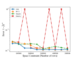
(a) U.S. Census

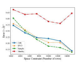
(b) YearPredictionMSD

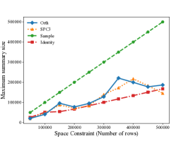
(c) Max summary size vs space constraint

Figure 2: Error vs Space Constraint in (a) and (b) and Maximum Summary Size vs Space Constraint (c). Total input size is $5000000\times 11$.

Results on approximation error compared to storage Let $f^{*}$ denote the minimal value of the full regression obtained by $x^{*}$ and let $x^{\prime}$ be the output of the reduced problem. The approximate solution to the full problem is then $\hat{f}=\|Ax^{\prime}-b\|_{\infty}$ and approximation error is measured as $\hat{f}/f^{*}-1$ (note that $\hat{f}\geq f^{*}$). An error closer to $0$ demonstrates that $\hat{f}$ is roughly the same as $f^{*}$ so the optimal value is well-approximated. Figures 2a and 2b show that on both datasets the Identity method consistently performs poorly while Sample achieves comparable accuracy to the conditioning methods. Despite the simplicity of uniform sampling to keep a summary, the succeeding sections discuss the increased time and space costs of using such a sample and show that doing so is not favourable. Thus, neither of the baseline methods output a summary which can be used to approximate the regression problem both accurately and quickly, hence justifying our use of leverage scores. Our conditioning methods perform particularly well in the US Census Data data (Figure 2a) with Orth appearing to give the most accurate summary and SPC3 performing comparably well but with slightly more fluctuation: similar behaviour is observed in the YearPredictionMSD (Figure 2b) data too. The conditioning methods are also seen to be robust to the storage constraint, give accurate performance across both datasets using significantly less storage than sampling, and give a better estimate in general than doing no conditioning.

Results on Space Complexity. Recall that the space constraint is $m$ rows and throughout the stream, after a local computation, the merge step concatenates more rows to the existing summary until the bound $m$ is met, prior to computing the next reduction. During the initialization of the block $A^{\prime}$ by Algorithm 1, the number of stored rows is exactly $m$. However, we measure the maximum number of rows kept in a summary after every reduction step to understand how large the returned summary can grow. As seen in Figure 2c, Identity keeps the smallest summary but there is no reason to expect it has kept the most important rows. In contrast, if $m$ is the bound on the summary size, then uniform sampling always returns a summary of size exactly $m$. However, we see that this is not optimal as both conditioning methods can return a set of rows which are pruned at every iteration to roughly half the size and contains only the most important rows in that block. Both conditioning methods exhibit similar behavior and are bounded between both Sample and Identity methods. Therefore, both of the conditioning methods respect the theoretical bound and, crucially, return a summary which is sublinear in the space constraint and hence a significantly smaller fraction of the input size.

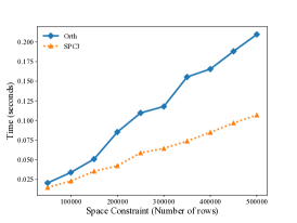
(a) Time to compute local basis

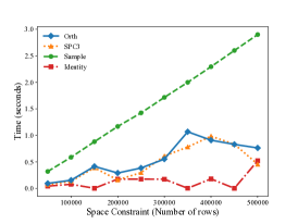
(b) Solution time for $\ell_{\infty}$-regression

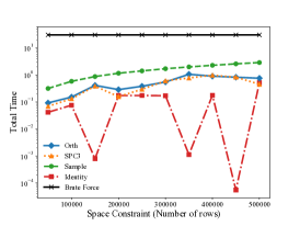
(c) Total time

Figure 3: Computation Times compared to summary size

Results on Time Complexity. There are three time costs measured. The first is the update time taken to compute the local well-conditioned basis which is theoretically $O(md^{2}+md^{5}\log m)$ by Theorem 2.2. However, the two bases that we test are an orthonormal basis, computable in time $O(md^{2})$ and the SPC3 transform which takes time $O(\text{nnz}(B)\log m)$ for a block $B$ with $m$ rows and $\text{nnz}(B)$ non-zero entries. Figure 3a demonstrates that SPC3 is faster than Orth on this data in practice but this small absolute difference becomes negligible over the entirety of the stream as seen in Figure 3c. The query time in Figure 3b is roughly proportional to the summary size in all instances but here the conditioning methods perform noticeably better due to the smaller summary size that is returned as discussed in the previous section. However, as seen in Figure LABEL:fig:_years_regression_time_vs_block_size.pdf, (Supplementary Material, Appendix LABEL:sec:_experimental_results_appendices ) this disparity becomes hugely significant on higher dimensionality data due to the increased size summary retained by sampling, further justifying our approach of pruning rows at every stage. While Identity appears to have fast query time, this is due to the summary being smaller. Although it may seem that for smaller summaries more local bases need to be computed and this time could prohibitively increase over the stream, Figure 3c demonstrates that even using small blocks does not cause the overall time (to process the stream and produce an approximate query) to increase too much. Hence, an approximation can be obtained which is highly accurate, and in total time faster than the brute force solver.

Experimental Summary. While it might seem attractive not to perform any conditioning on the matrix and just pick heavy rows, our experiments show that this strategy is not effective in practice, and delivers poor accuracy. Although a simple sample of randomly chosen rows can be easily maintained, this appears less useful due to the increased time costs associated with larger summaries when conditioning methods output a similar estimate in less time over the entire stream. As the $\ell_{\infty}$-regression problems depend only on a few rows of the data there are cases when uniform sampling can perform well: if many of the critical rows look similar then there is a chance that uniform sampling will select some examples. In this case, the leverage of the important direction is divided across the repetitions, and so it is harder to ensure that desired direction is identified. Despite this potential drawback we have shown that both Orth and SPC3 can be used to find accurate summaries which perform robustly across each of the measures we have tested. It appears that SPC3 performs comparably to Orth; both are relatively quick to compute and admit accurate summaries in similar space. In particular, both conditioning methods return summaries which are a fraction of the space budget and hence highly sublinear in the input size, which give accurate approximations and are robust to the concatenation of new rows. All of these factors make the conditioning method fast in practice to both find the important rows in the data and then compute the reduced regression problem with high accuracy.

Due to the problems in constructing summaries which can be used to solve regression quickly and accurately when using random sampling or no transformation, our methods are shown to be efficient and accurate alternatives. Our approach is vindicated both theoretically and practically: this is most clear in the U.S. Census dataset where small error can be achieved using a summary roughly $2\%$ the size of the data. This also results in an overall speedup as solving the optimization on the reduced set is much faster than solving on the full problem. Such significant savings show that this general approach can be useful in large-scale applications.

Supplementary Material for Leveraging Well-Conditioned Bases: Streaming and
Distributed Summaries in Minkowski $p$-Norms

Appendix A Proofs for Section 3

Lemma A.1.

Denote the $i$th global leverage score of $A$ by $w_{i}$ and its associated local leverage score in a block of input $A$ be denoted $\hat{w}_{k}$. Then $w_{i}/\text{poly}(d)\leq\hat{w}_{k}$. In particular, $w_{i}/(d\alpha^{p}\beta)\leq\hat{w}_{k}$.

Proof of Lemma A.1..

Let $U=AR$. Recall that $w_{i}=\|\mathbf{e}_{i}^{T}AR\|_{p}^{p}$. Then for some coordinate $j$ we must have $|\mathbf{e}_{i}^{T}AR\mathbf{e}_{j}|^{p}\geq w_{i}/d$. Taking $\mathbf{x}=\mathbf{e}_{j}$ we see that

$$|(AR\mathbf{x})_{i}|^{p}\geq\frac{w_{i}}{d}.$$ (2)

However, Fact 1 implies :

$$\|AR\mathbf{x}\|_{p}^{p}\leq\|AR\|_{p}^{p}\leq\alpha^{p}\leq\text{poly}(d).$$ (3)

Hence, there exists a $\mathbf{y}\in\text{col}(A)$ with $\mathbf{y}=AR\mathbf{x}$ such that $|\mathbf{y}_{i}|^{p}\geq w_{i}/d$ from Equation (2). Also, $\|\mathbf{y}\|_{p}^{p}\leq\alpha^{p}$ from Equation (3). Thus,

$$\frac{|\mathbf{y}_{i}|^{p}}{\|\mathbf{y}\|_{p}^{p}} \geq\frac{|\mathbf{y}_{i}|^{p}}{\alpha^{p}}$$ (4)

$$\geq\frac{w_{i}}{d\alpha^{p}}$$ (5)

$$\geq\frac{w_{i}}{\text{poly}(d)}.$$ (6)

From this we see;

$$w_{i}\leq\frac{|\mathbf{y}_{i}|^{p}d\alpha^{p}}{\|\mathbf{y}\|_{p}^{p}}.$$ (7)

Now, let $B$ be a block of rows from $A$. We manipulate $B$ by considering it either as an individual matrix or as a coordinate subspace of $A$; i.e all rows are zero except for those contained in $B$ which will be denoted by $\hat{A}$. Define $\hat{\mathbf{y}}=\hat{A}R\mathbf{x}$. Then $\hat{\mathbf{y}}_{j^{\prime}}=\mathbf{y}_{j^{\prime}}$ when $j^{\prime}$ is a row from $B$ and $\hat{\mathbf{y}}_{j^{\prime}}=0$ otherwise. Thus, $\|\hat{\mathbf{y}}\|_{p}^{p}\leq\|\mathbf{y}\|_{p}^{p}$ and:

$$w_{i}\leq\frac{|\mathbf{y}_{i}|^{p}d\alpha^{p}}{\|\hat{\mathbf{y}}\|_{p}^{p}}.$$ (8)

For rows $i$ which are also found in $B$ (indexed as $k$) we see that $|\hat{\mathbf{y}}_{k}|^{p}=|\mathbf{y}_{i}|^{p}$. So, for such indices, using Equations (7) and (8):

$$w_{i}\leq\frac{|\hat{\mathbf{y}}_{k}|^{p}d\alpha^{p}}{\|\hat{\mathbf{y}}\|_{p}^{p}}.$$ (9)

Since $\hat{\mathbf{y}}$ is the restriction of $\mathbf{y}$ to coordinates of $B$ we can write $\hat{\mathbf{y}}=B\hat{R}\hat{x}$ where $B\hat{R}$ is well-conditioned. Let $\hat{w}_{k}=\|\mathbf{e}_{k}^{T}B\hat{R}\|_{p}^{p}$ be the $k$th local leverage score in $B$. By applying the same argument as in Fact 2 it can be shown that $|\hat{\mathbf{y}}_{k}|^{p}/\|\hat{\mathbf{y}}\|_{p}^{p}\leq\text{poly}(d)\hat{w}_{k}$. Indeed,

$$|\hat{\mathbf{y}}_{k}|^{p} =|(\hat{A}\hat{R}\hat{x})_{k}|^{p}$$ (10)

$$\leq\|e_{k}^{T}\hat{A}\hat{R}\|_{p}^{p}\|\hat{x}\|_{q}^{p}\text{\quad by H\"{o}lder's inequality}$$ (11)

$$\leq\hat{w}_{k}\beta\|B\hat{R}\hat{x}\|_{p}^{p}$$ (12)

$$\leq\beta\hat{w}_{k}\|\hat{\mathbf{y}}\|_{p}^{p}.$$ (13)

The second inequality uses condition 2 from Theorem 2.1 and the fact that $B\hat{R}$ is a well-conditioned basis. Then using Equation 9, the following then proves the latter claim of the lemma:

$$\frac{w_{i}}{d\alpha^{p}}\leq\frac{|\hat{\mathbf{y}}_{k}|^{p}}{\|\hat{\mathbf{y}}\|_{p}^{p}}\leq\beta\hat{w}_{k}.$$

Finally, Theorem 2.2 states that $\beta$ is at most $\text{poly}(d)$ which proves the result. ∎

Lemma A.2.

All global leverage scores above a threshold can be found by computing local leverage scores and increasing the space complexity by a $\text{poly}(d)$ factor.

Proof of Lemma A.2..

First we determine the space necessary to find all leverage scores exceeding $\delta$. Let $I=\{i:w_{i}>\delta\}$. Then $\alpha^{p}\geq\sum_{i=1}^{n}w_{i}\geq\sum_{i\in I}w_{i}\geq\delta|I|$ by arguing as in Fact 1 Hence, the space necessary is $|I|\leq\alpha^{p}/\delta$. Now focus on finding these rows in the streaming fashion. By Lemma A.1 we see that for rows $k$ in the block which is stored from the stream we have the property that $w_{i}/d\alpha^{p}\beta\leq\hat{w}_{k}$. Hence, any $w_{i}>\delta$ results in $\hat{w}_{k}>\delta/d\alpha^{p}\beta$ for the local thresholding. So to keep all such $w_{i}>\delta$, we must store all $\hat{w}_{k}>\delta/d\alpha^{p}\beta=\hat{\delta}$. Arguing similarly as in Fact 1 again define $\hat{I}=\{k:\hat{w}_{k}>\hat{\delta}\}$ so that: $\alpha^{p}\geq\sum_{k}\hat{w}_{k}\geq\sum_{k\in\hat{I}}\hat{w}_{k}\geq\hat{\delta}|\hat{I}|$. Hence $|\hat{I}|\leq\alpha^{p}/\hat{\delta}=d\alpha^{2p}\beta/\delta$. That is, $|\hat{I}|\leq d\beta\alpha^{p}\cdot|I|$ which proves the claim as Theorem 2.2 states that all of the parameters are $\text{poly}(d)$. ∎

Proof of Theorem 3.3..

We claim that the output of Algorithm 1 is a matrix $B$ which contains rows of high leverage in $A$. The algorithm initially reads in $b$ rows and inserts these to matrix $A^{\prime}$. A well-conditioned basis $U$ for $A^{\prime}$ is then computed using Theorem 2.2 and incurs the associated $O(bd^{2}+bd^{5}\log b)$ time. The matrix $U$ and $A^{\prime}$ are passed to Algorithm 2 whereby if a row $i$ in $U$ has local leverage exceeding $\tau$ then row $i$ of $A^{\prime}$ is kept. There are at most $\text{poly}(d)/\tau$ of these rows as seen in Lemma A.2 and the space required is $\text{poly}(d)$ by the same lemma. So on the first call to Algorithm 2 a matrix is returned with rows whose $\ell_{p}$ local leverage satisfies $w_{i}/\text{poly}(d)\leq\hat{w}_{i}$ (where $w_{i}$ is the global leverage score and $\hat{w}_{i}$ is the associated local leverage score) and only those exceeding $\tau/\operatorname{poly}(d)$ are kept.

The algorithm proceeds by repeating this process on a new set of rows from $A$ and an improved matrix $B$ which contains high leverage rows from $A$ already found. Proceeding inductively, we see that when Algorithm 2 is called with matrix $[A^{\prime};B]$ then a well-conditioned basis $U$ is computed. Again $[A^{\prime};B]_{i}$ is kept if and only if the local leverage score from $U$, $w_{i}(U)>\tau$. By Lemma A.2 this requires $\text{poly}(d)$ space and the local leverage score is at least a $1/\text{poly}(d)$ factor as large as the global leverage score by Lemma A.1. Repeating over all blocks $B$ in $A$, only the rows of high leverage are kept. Any row of leverage smaller than $\tau/\text{poly}(d)$ is ignored so this is the additive error incurred. ∎

Appendix B Proofs for Section 4

Algorithm and Discussion

The pseudocode for the first level of the tree structure of the deterministic $\ell_{p}$ subspace embedding described in Section 4 is given in Algorithm 3. We use the following notation: $m$ is a counter to index the block of input currently held, denoted $A_{[m]}$, and ranges from $1$ to $n^{1-\gamma}$ for the first level of the tree. Similarly, $t$ indexes the current summary, $P^{(t)}$ which are all initialized to be an empty matrix. Again we use the notation $[X;Y]$ to denote the row-wise concatenation of two matrices $X$ and $Y$ with equal column dimension.

Note that Algorithm 3 can be easily distributed as any block of sublinear size can be given to a compute node and then a small-space summary of that block is returned to continue the computation. In addition, the algorithm can be performed using sublinear space in the streaming model because at any one time a summary $T$ of the input can be computed which is of size $d\times d$. Upon reading $A_{[1]}$, a small space summary $P^{(1)}$ is computed and stored with the algorithm proceeding to read in $A_{[2]}$. Similarly, the summary $P^{(2)}$ is computed and if $[P^{(1)};P^{(1)}]$ does not exceed the storage bound, then the two summaries are merged and this process is repeated until at some point the storage bound is met. Once the summary is large enough that it meets the storage bound, it is then reduced by performing the well-conditioned basis reduction (line (3)) and the reduced summary is stored with the algorithm continuing to read and summarize input until a corresponding block in the tree is obtained (or the blocks can be combined to terminate the algorithm).

Algorithm 3 Deterministic $\ell_{p}$ subspace embedding

$\ell_{p}$-SubspaceEmbedding$A,p,\gamma<1)$Counters $m,t\leftarrow 1$Summaries $P^{(t)}\leftarrow\text{EMPTY}$for all $t$. $m=1:n^{1-\gamma}$$A_{[m]}=US$# $U$an $\ell_{p}$wcb for $A$$\text{num. rows}(P^{(t)})+d\leq n^{\gamma}$$P^{(t)}\leftarrow[P^{(t)};S]$$P^{(t+1)}\leftarrow S$$t\leftarrow t+1$Mergeall $P^{(t)}$: $T=[P^{(1)};\ldots;P^{(\cdot)}]$Reduce$T$by splitting into blocks of $n^{\gamma}$

References

- Agarwal et al. (2012) Agarwal, Pankaj, Cormode, Graham, Huang, Zengfeng, Phillips, Jeff, Wei, Zheiwei, and Yi, Ke. Mergeable summaries. In ACM Principles of Database Systems, 2012.
- Clarkson et al. (2013) Clarkson, K. L., Drineas, P., Magdon-Ismail, M., Mahoney, M. W., Meng, X., and Woodruff, D. P. The fast cauchy transform and faster robust linear regression. In Proc. of the 24-th Annual SODA, pp. 466–477, 2013.
- Cohen & Peng (2015) Cohen, Michael B and Peng, Richard. row sampling by lewis weights. In Proceedings of the forty-seventh annual ACM symposium on Theory of computing, pp. 183–192. ACM, 2015.
- Dasgupta et al. (2008) Dasgupta, A., Drineas, P., Harb, B., Kumar, R., and Mahoney, M. W. Sampling algorithms and coresets for regression. In Proc. of the 19th Annual SODA, pp. 932–941, 2008.
- Feldman et al. (2006) Feldman, Jon, Muthukrishnan, S., Sidiropoulos, Anastasios, Stein, Cliff, and Svitkina, Zoya. On the complexity of processing massive, unordered, distributed data. Technical Report CoRR abs/cs/0611108, ArXiV, 2006.
- Ghashami et al. (2016) Ghashami, M., Liberty, E., and Phillips, J. M. Efficient Frequent Directions Algorithm for Sparse Matrices. ArXiv e-prints, 2016.
- Ghashami & Phillips (2014) Ghashami, Mina and Phillips, Jeff M. Relative errors for deterministic low-rank matrix approximations. In Proceedings of the Twenty-Fifth Annual ACM-SIAM Symposium on Discrete Algorithms, SODA 2014, Portland, Oregon, USA, January 5-7, 2014, pp. 707–717, 2014.
- Ghashami et al. (2016) Ghashami, Mina, Liberty, Edo, Phillips, Jeff M., and Woodruff, David P. Frequent directions: Simple and deterministic matrix sketching. SIAM J. Comput., 45(5):1762–1792, 2016.
- Hand (1978) Hand, Michael Lawrence. Aspects of linear regression estimation under the criterion of minimizing the maximum absolute residual. 1978.
- Hardt & Woodruff (2013) Hardt, Moritz and Woodruff, David P. How robust are linear sketches to adaptive inputs? In Proceedings of the Forty-fifth Annual ACM Symposium on Theory of Computing, STOC ’13, pp. 121–130, New York, NY, USA, 2013. ACM. ISBN 978-1-4503-2029-0. doi: 10.1145/2488608.2488624. URL http://doi.acm.org/10.1145/2488608.2488624.
- Kremer et al. (1999) Kremer, Ilan, Nisan, Noam, and Ron, Dana. On randomized one-round communication complexity. Computational Complexity, 8(1):21–49, 1999.
- Kushilevitz & Nisan (1997) Kushilevitz, E. and Nisan, N. Communication Complexity. Cambridge University Press, 1997.
- Liberty (2013) Liberty, Edo. Simple and deterministic matrix sketching. In The 19th ACM SIGKDD International Conference on Knowledge Discovery and Data Mining, KDD 2013, Chicago, IL, USA, August 11-14, 2013, pp. 581–588, 2013.
- Meng & Mahoney (2013) Meng, Xiangrui and Mahoney, Michael W. Low-distortion subspace embeddings in input-sparsity time and applications to robust linear regression. In Symposium on Theory of Computing Conference, STOC’13, Palo Alto, CA, USA, June 1-4, 2013, pp. 91–100, 2013.
- Shen et al. (2014) Shen, Fumin, Shen, Chunhua, Hill, Rhys, van den Hengel, Anton, and Tang, Zhenmin. Fast approximate minimization: speeding up robust regression. Computational Statistics & Data Analysis, 77:25–37, 2014.
- Song et al. (2017) Song, Z., Woodruff, D., and Zhong, P. Low rank approximation with entrywise -norm error. In STOC, 2017.
- Sposito (1976) Sposito, VA. Minimizing the maximum absolute deviation. ACM SIGMAP Bulletin, (20):51–53, 1976.
- Woodruff (2014) Woodruff, David. Sketching as a tool for numerical linear algebra. Foundations and Trends in Theoretical Computer Science, 10(1-2):1–157, 2014.
- Woodruff & Zhang (2013) Woodruff, David and Zhang, Qin. Subspace embeddings and -regression using exponential random variables. JMLR: Workshop and Conference Proceedings, 30:1–22, 2013.
- Yang et al. (2013) Yang, J., Meng, X., and Mahoney, M. W. Quantile regression for large-scale applications. Proc. of the 30th ICML Conference, JMLR W&CP, 28(3):881–887, 2013.