Updating Probabilistic Knowledge on Condition/Event Nets using Bayesian Networks

Abstract.

The paper extends Bayesian networks (BNs) by a mechanism for dynamic changes to the probability distributions represented by BNs. One application scenario is the process of knowledge acquisition of an observer interacting with a system. In particular, the paper considers condition/event nets where the observer’s knowledge about the current marking is a probability distribution over markings. The observer can interact with the net to deduce information about the marking by requesting certain transitions to fire and observing their success or failure.

Aiming for an efficient implementation of dynamic changes to probability distributions of BNs, we consider a modular form of networks that form the arrows of a free PROP with a commutative comonoid structure, also known as term graphs. The algebraic structure of such PROPs supplies us with a compositional semantics that functorially maps BNs to their underlying probability distribution and, in particular, it provides a convenient means to describe structural updates of networks.

1. Introduction

Representing uncertain knowledge by probability distributions is the core idea of Bayesian learning. We model the potential of an agent—the observer—interacting with a concurrent system with hidden or uncertain state to gain knowledge through “experimenting” with the system, focussing on the problem of keeping track of knowledge updates correctly and efficiently. Knowledge about states is represented by a probability distribution. Our system models are condition/even nets where states or possible worlds are markings and transitions describe which updates are allowed.

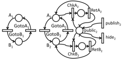
Figure 1. Example: Social network account with location privacy

In order to clarify our intentions we consider an application scenario from social media: preventing inadvertent disclosure, which is the concern of location privacy [7]. Consider the example of a social network account, modelled as a condition/event net, allowing a user to update and share their location (see Figure 1). We consider two users. User 1 does not allow location updates to be posted to the social network, they are only recorded on their device. In the net this is represented by places $\mathsf{A_{1}}$ and $\mathsf{B_{1}}$ modelling the user at corresponding locations, and transitions $\mathsf{GotoA_{1}}$ and $\mathsf{GotoB_{1}}$ for moving between them. We assume that only User 1 can fire or observe these transitions. User 2 has a similar structure for locations and movements, but allows the network to track their location. The user can decide to make their location public or hide it by firing transition $\mathsf{publish_{2}}$ or $\mathsf{hide_{2}}$. Any observer can attempt to fire $\mathsf{ChkA_{2};RetA_{2}}$ or $\mathsf{ChkB_{2};RetB_{2}}$ to query the current location of User 2. If $\mathsf{public_{2}}$ is marked, this will allow the observer to infer the correct location. Otherwise the observer is left uncertain as to why the query fails, i.e. due to the wrong location being tested or the lack of permission, unless they test both locations. While our net captures the totality of possible behaviours, we identify different observers, the two users, the social network, and an unrelated observer. For each of these we define which transitions they can access. We then focus on one observer and only allow transitions they are authorised for. In our example, if we want to analyse the unrelated observer, we fix the users’ locations and privacy choices before it is the observer’s turn to query the system.

The observer may have prior knowledge about the dependencies between the locations of Users 1 and 2, for example due to photos with location information published by User 2, in which both users may be identifiable. The prior knowledge is represented in the initial probability distribution, updated according to the observations.

We also draw inspiration from probabilistic databases [27, 1] where the values of attributes or the presence of records are only known probabilistically. However, an update to the database might make it necessary to revise the probabilities. Think for instance of a database where the gender of a person (male or female) is unknown and we assume with probability $1/2$ that they are male. Now a record is entered, stating that the person has married a male. Does it now become more probable that the person is female?

Despite its simplicity, our system model based on condition/event nets allows us to capture databases: the content of a database can be represented as a (hyper-)graph (where each record is a (hyper-)edge). If the nodes of the graph are fixed, updates can be represented by the transitions of a net, where each potential record is represented by a place.

Given a net, the observer does not know the initial marking, but has a prior belief, given by a probability distribution over markings. The observer can try to fire transitions and observe whether the firing is successful or fails. Then the probability distribution is updated accordingly. While the update mechanism is rather straightforward, the problem lies in the huge number of potential states: we have $2^{n}$ markings if $n$ is the number of places.

To mitigate this state space explosion, we propose to represent the observer’s knowledge using Bayesian networks (BNs) [21, 23], i.e., graphical models that record conditional dependencies of random variables in a compact form. However, we encounter a new problem as updating the observer’s knowledge becomes non-trivial. To do this correctly and efficiently, we develop a compositional approach to BNs based on symmetric monoidal theories and PROPs [19]. In particular, we consider modular Bayesian networks as arrows of a freely generated PROP and (sub-)stochastic matrices as another PROP with a functor from the former to the latter. In this way, we make Bayesian networks compositional and we obtain a graphical formalism [26] that we use to modify Bayesian networks: in particular, we can replace entire subgraphs of Bayesian networks by equivalent ones, i.e., graphs that evaluate to the same matrix. The compositional approach allows us to specify complex updates in Bayesian networks by a sequence of simpler updates using a small number of primitives.

We furthermore describe an implementation and report promising runtime results.

The proofs of all results can be found in Appendix A.

2. Knowledge Update in Condition/Event Nets

We will formalise knowledge updates by means of an extension of Petri nets with probabilistic knowledge on markings. The starting point are condition/event nets [25].

Definition 1 (Condition/event net).

A condition/event net (CN) $N=(S,T,\prescript{\bullet}{}{()},{()}^{\bullet},m_{0})$ is a five-tuple consisting of a finite set of places $S$, a finite set of transitions $T$ with pre-conditions $\prescript{\bullet}{}{()}:T\rightarrow\mathcal{P}(S)$, post-conditions ${()}^{\bullet}:T\rightarrow\mathcal{P}(S)$, and $m_{0}\subseteq S$ an initial marking. A marking is any subset of places $m\subseteq S$. We assume that for any $t\in T$, $\prescript{\bullet}{}{t}\cap{t}^{\bullet}=\emptyset$.

A transition $t$ can fire for a marking $m\subseteq S$, denoted $m\Rightarrow^{t}$, if $\prescript{\bullet}{}{t}\subseteq m$ and ${t}^{\bullet}\cap m=\emptyset$. Then marking $m$ is transformed into $m^{\prime}=(m\setminus\prescript{\bullet}{}{t})\cup{t}^{\bullet}$, written $m\Rightarrow^{t}m^{\prime}$. We write $m\Rightarrow^{t}$ to indicate that there exists some $m^{\prime}$ with $m\Rightarrow^{t}m^{\prime}$.

We will use two different notations to indicate that a transition cannot fire, the first referring to the fact that the pre-condition is not sufficiently marked, the second stating that there are tokens in the post-condition: $m\not\Rightarrow^{t}_{\mathit{pre}}$ whenever $\prescript{\bullet}{}{t}\not\subseteq m$ and $m\not\Rightarrow^{t}_{\mathit{post}}$ whenever ${t}^{\bullet}\cap m\neq\emptyset$. We denote the set of all markings by $\mathcal{M}=\mathcal{P}(S)$.

For simplicity we assume that $S=\{1,\dots,n\}$ for $n\in\mathbb{N}$. Then, a marking $m$ can be characterized by a boolean vector $m:S\rightarrow\{0,1\}$, i.e., $\mathcal{M}\cong\{0,1\}^{S}$. Using the vector notation we write $m(A)=\{1\}$ for $A\subseteq S$ if all places in $A$ are marked in $m$.

To capture the probabilistic observer we augment CNs by a probability distribution over markings modelling uncertainty about the hidden initial or current marking.

Definition 2 (Condition/Event net with Uncertainty).

A Condition/Event Net with Uncertainty (CNU) is a six-tuple $N=(S,T,\prescript{\bullet}{}{()},{()}^{\bullet},m_{0},p)$ where $(S,T,\prescript{\bullet}{}{()},{()}^{\bullet},m_{0})$ is a net as in Definition 1. Additionally, $p$ is a function $p:\mathcal{M}\rightarrow[0,1]$ with $\sum_{m\in\mathcal{M}}p(m)=1$ that assigns a probability mass to each possible marking. This gives rise to a probability space $(\mathcal{M},\mathcal{P}(\mathcal{M}),\mathbb{P})$ with $\mathbb{P}:\mathcal{P}(\mathcal{M})\rightarrow[0,1]$ defined by $\mathbb{P}\bigl{(}\{m_{1},\dots,m_{k}\}\bigr{)}=\sum_{i=1}^{k}p(m_{i})$.

We assume that $p(m_{0})>0$, i.e. the initial marking is possible according to $p$.

We model the knowledge gained by observers when firing transitions and observing their outcomes. Firing $t\in T$ can either result in success (all places of $\prescript{\bullet}{}{t}$ are marked and no place in ${t}^{\bullet}$ is marked) or in failure (at least one place of $\prescript{\bullet}{}{t}$ is empty or one place in ${t}^{\bullet}$ is marked). Thus, there are two kinds of failure, the absence of tokens in the pre-condition or the presence of tokens in the post-condition. If a transition fails for both reasons, the observer will learn only one of them. To model the knowledge gained we define the following operations on distributions. inline] R1: must none of the places of ${t}^{\bullet}$ be marked for t to be successful? It seems like the fail_post condition implies this, but it is not stated as a success condition.
Ben: [DONE] I think it is explicitly stated in the previous sentences and we should not change anything

Definition 3 (Operations on CNUs).

Given a CNU $N=(S,T,\prescript{\bullet}{}{()},{()}^{\bullet},m_{0},p)$ the following operations update the mass function $p$ and as a result the probability distribution $\mathbb{P}$.

• To assert that certain places $A\subseteq S$ all contain a token ($b=1$) or that none contains a token ($b=0$) we define the operation assert

  $$\mathrm{ass}_{A,b}(p)(m)=\frac{p(m)}{\sum_{m^{\prime}\in\mathcal{M}:m^{\prime}(A)=\{b\}}p(m^{\prime})},\text{ if }m(A)=\{b\}\qquad\text{and}\quad 0,\text{ otherwise. }$$ (1)

• To state that at least one place of a set $A\subseteq S$ does (resp. does not) contain a token we define operation negative assert

  $$\mathrm{nas}_{A,b}(p)(m)=\frac{p(m)}{\sum_{m^{\prime}\in\mathcal{M}:m^{\prime}(A)\neq\{b\}}p(m^{\prime})},\text{ if }m(A)\neq\{b\}\quad\text{and}\quad 0,\text{ otherwise. }$$ (2)

• Modifying a set of places $A\subseteq S$ such that all places contain a token ($b=1$) or none contains a token ($b=0$) requires the following operation

  $$\mathrm{set}_{A,b}(p)(m)={\sum_{m^{\prime}:m^{\prime}|_{S\setminus A}=m|_{S\setminus A}}}p(m^{\prime}),\text{ if }m(A)=\{b\}\quad\text{and}\quad 0,\text{ otherwise}.$$ (3)

• A successful firing of a transition $t$ leads to an assert ($\mathrm{ass}$) and $\mathrm{set}$ of the pre-conditions $\prescript{\bullet}{}{t}$ and the post-conditions ${t}^{\bullet}$. A failed firing translates to a negative assert ($\mathrm{nas}$) of the pre- or post-condition and nothing is set. Thus we define for a transition $t\in T$

  $$\mathrm{success}_{t}(p) =\mathrm{set}_{{t}^{\bullet},1}(\mathrm{set}_{\prescript{\bullet}{}{t},0}(\mathrm{ass}_{{t}^{\bullet},0}(\mathrm{ass}_{\prescript{\bullet}{}{t},1}(p)))) \mathrm{fail}^{\mathit{pre}}_{t}(p) =\mathrm{nas}_{\prescript{\bullet}{}{t},1}(p)$$

  $$\mathrm{fail}^{\mathit{post}}_{t}(p) =\mathrm{nas}_{{t}^{\bullet},0}(p).$$

Operations $\mathrm{ass},\mathrm{nas}$ are partial, defined whenever the sum in the denominator of their first clause is greater than $0$. That means, the observer only fires transitions whose pre- and postconditions have a probability greater than zero, i.e., where according to their knowledge about the state it is possible that these transitions are enabled. By Definition 1 the initial marking is possible, and this property is maintained as markings and distributions are updated. If this assumption is not satisfied, the operations in Definition 3 are undefined.

The $\mathrm{ass}$ and $\mathrm{nas}$ operations result from conditioning the input distribution on (not) having tokens at $A$ (compare Proposition 4). Also, $\mathrm{set}$ and $\mathrm{ass}$ for $A=\{s_{1},\dots,s_{k}\}\subseteq S$ can be performed iteratively, i.e., $\mathrm{set}_{A,b}=\mathrm{set}_{\{s_{k}\},b}\circ\dots\circ\mathrm{set}_{\{s_{1}\},b}$ and $\mathrm{ass}_{A,b}=\mathrm{ass}_{\{s_{k}\},b}\circ\dots\circ\mathrm{ass}_{\{s_{1}\},b}$. For a single place $s$ we have $\mathrm{ass}_{\{s\},b}=\mathrm{nas}_{\{s\},1-b}$.

Figure 2 gives an example for a Petri net with uncertainty and explains how the observer can update their knowledge by interacting with the net.

– places –				$\mathit{success}_{t_{4}}$				$\mathit{fail}^{\mathit{pre}}_{t_{1}}$
$S_{1}$	$S_{2}$	$S_{3}$	init	$\mathrm{as}_{\{S_{2}\},1}$	$\mathrm{as}_{\{S_{3}\},0}$	$\mathrm{set}_{\{S_{2}\},0}$	$\mathrm{set}_{\{S_{3}\},1}$	$\mathrm{nas}_{\{S_{1}\},1}$
$1$	$1$	$1$	$\nicefrac{{1}}{{12}}$	$\nicefrac{{1}}{{6}}$	$0$	$0$	$0$	$0$
$1$	$1$	$0$	$\nicefrac{{1}}{{6}}$	$\nicefrac{{1}}{{3}}$	$\nicefrac{{1}}{{2}}$	$0$	$0$	$0$
$1$	$0$	$1$	$\nicefrac{{1}}{{8}}$	$0$	$0$	$0$	$\nicefrac{{1}}{{2}}$	$0$
$1$	$0$	$0$	$\nicefrac{{1}}{{8}}$	$0$	$0$	$\nicefrac{{1}}{{2}}$	$0$	$0$
$0$	$1$	$1$	$\nicefrac{{1}}{{12}}$	$\nicefrac{{1}}{{6}}$	$0$	$0$	$0$	$0$
$0$	$1$	$0$	$\nicefrac{{1}}{{6}}$	$\nicefrac{{1}}{{3}}$	$\nicefrac{{1}}{{2}}$	$0$	$0$	$0$
$0$	$0$	$1$	$\nicefrac{{1}}{{8}}$	$0$	$0$	$0$	$\nicefrac{{1}}{{2}}$	$1$
$0$	$0$	$0$	$\nicefrac{{1}}{{8}}$	$0$	$0$	$\nicefrac{{1}}{{2}}$	$0$	$0$

Figure 2. Example of operations on a net with uncertainty. We set $m_{0}=\{S_{2}\}$ and assume the observer first fires $t_{4}$ (and succeeds) and then tries to fire $t_{1}$ (and fails). Columns in the table represent updated distributions on the markings after each operation (ordered from left to right). For this example, in the end the observer knows that the final configuration is $\{S_{3}\}$ with probability $1$.

inline] R1: Figure 2: last column of the table seems wrong, should the 1 be in the row corresponding to 001 (instead of 101)?
Ben: [DONE] He/She is right. I moved the 1 to the correct spot inline] R1: Also, it would be nice to explicitly state each column [in Fig. 2] is the result of applying the operation in the header to the column immediately to the left.
Ben: [DONE] I changed one sentence in the caption of Fig. 2 We can now show that our operations correctly update the probability assumptions according to the observations of the net.

Proposition 4.

Let $N=(S,T,\prescript{\bullet}{}{()},{()}^{\bullet},m_{0},p)$ be a CNU where $\mathbb{P}$ is the corresponding probability distribution. For given $t\in T$ and $m\in\mathcal{M}$ let $\mathcal{M}[\Rightarrow^{t}]=\{m^{\prime}\in\mathcal{M}\mid m^{\prime}\Rightarrow^{t}\}$, $\mathcal{M}[\Rightarrow^{t}m]=\{m^{\prime}\in\mathcal{M}\mid m^{\prime}\Rightarrow^{t}m\}$, $\mathcal{M}[\not\Rightarrow^{t}_{\textit{pre}}]=\{m^{\prime}\in\mathcal{M}\mid m^{\prime}\not\Rightarrow^{t}_{\mathit{pre}}\}$ and $\mathcal{M}[\not\Rightarrow^{t}_{\textit{post}}]=\{m^{\prime}\in\mathcal{M}\mid m^{\prime}\not\Rightarrow^{t}_{\mathit{post}}\}$. Then, provided that $\mathcal{M}[\Rightarrow^{t}]$, $\mathcal{M}[\not\Rightarrow^{t}_{\textit{pre}}]$ respectively $\mathcal{M}[\not\Rightarrow^{t}_{\textit{post}}]$ are non-empty, it holds for $m\in\mathcal{M}$ that

$$\mathrm{success}_{t}(p)(m) =\mathbb{P}(\mathcal{M}[\Rightarrow^{t}m]\mid\mathcal{M}[\Rightarrow^{t}]) \mathrm{fail}^{\mathit{pre}}_{t}(p)(m) =\mathbb{P}(\{m\}\mid\mathcal{M}[\not\Rightarrow^{t}_{\textit{pre}}])$$

$$\mathrm{fail}^{\mathit{post}}_{t}(p)(m) =\mathbb{P}(\{m\}\mid\mathcal{M}[\not\Rightarrow^{t}_{\textit{post}}])$$

inline] R1: it’s clear what is meant from context, but I don’t think the notation $m^{\prime}\Rightarrow^{t}$ was ever defined.
Ben: [DONE] I added the notation $m\Rightarrow^{t}$ in Definition 1. Please check.

We shall refer to the the joint distribution (over all places) by $\mathbb{P}$. Note that it is unfeasible to explicitly store it if the number of places is large. To mitigate this problem we use a Bayesian network with a random variable for each place, recording dependencies between the presence of tokens in different places. If such dependencies are local, the BN is often moderate in size and thus provides a compact symbolic representation. However, updating the joint distribution of BNs is non-trivial. To address this problem, we propose a propagation procedure based on a term-based, modular representation of BNs.

3. Modular Bayesian Networks and Sub-Stochastic Matrices

Bayesian networks (BNs) are a graphical formalism to reason about probability distributions. They are visualized as directed, acyclic graphs with nodes random variables and edges dependencies between them. inline] R1:“the probability distribution of Figure 2” – Figure 2 has many probability distributions; perhaps it’s clearer to refer explicitly to ’init’
Ben: [DONE] I removed the sentence “An example BN, encoding the probability distribution of Figure 2 is given in Figure 5.” completely and in Figure 5 I added “initial” to distribution. This is sufficient for static BNs whose most common operation is the inference of (marginalized or conditional) distributions of the underlying joint distribution.

For a rewriting calculus on dynamic BNs, we consider a modular representation of networks that do not only encode a single probability vector, but a matrix, with several input and output ports. The first aim is compositionality: larger nets can be composed from smaller ones via sequential and parallel composition, which correspond to matrix multiplication and Kronecker product of the encoded matrices. This means, we can implement the operations of Section 2 in a modular way.

PROPs with Commutative Comonoid Structure

We now describe the underlying compositional structure of (modular) BNs and (sub-)stochastic matrices, which facilitates a compositional computation of the underlying probability distribution of (modular) BNs. The mathematical structure are PROPs [19] (see also [12, Chapter 5.2]), i.e., strict symmetric monoidal categories $(C,\otimes,0,\sigma)$ whose objects are (in bijection with) the natural numbers, with monoidal product $\otimes$ as (essentially) addition, with unit $0$. The compositional structure of PROPs can be intuitively represented using string diagrams with wires and boxes (see Figure 3). Symmetries $\sigma$ serve for the reordering of wires.

$\leavevmode\hbox to59.94pt{\vbox to21.94pt{\text{[drawing]}}}=\leavevmode\hbox to68.9pt{\vbox to21.94pt{\text{[drawing]}}}$

$\leavevmode\hbox to117.74pt{\vbox to22.11pt{\text{[drawing]}}}=\begin{array}[c]{c}\leavevmode\hbox to50.6pt{\vbox to21.94pt{\text{[drawing]}}}\nobreak\leavevmode\\[8.61108pt] \leavevmode\hbox to50.6pt{\vbox to21.94pt{\text{[drawing]}}}\end{array}$

Figure 3. String diagrammatic composition (resp. tensor) of two arrows $f\colon m\to n$, $f^{\prime}\colon n\to k$ (resp. $f_{1}\colon m_{1}\to n_{1}$, $f_{2}\colon m_{2}\to n_{2}$) of a PROP $(C,\otimes,0,\sigma)$

A paradigmatic example is the PROP of $2^{n}$-dimensional Euclidean spaces and linear maps, equipped with the tensor product: the tensor product of $2^{n}$- and $2^{m}$-dimensional spaces is $2^{n+m}$-dimensional, composition of linear maps amounts to matrix multiplication, and the tensor product is also known as Kronecker product (as detailed below). We refer to the natural numbers of the domain and codomain of arrows in a PROP as their type; thus, a linear map from $2^{n}$- to $2^{m}$-dimensional Euclidean space has type $n\to m$.

We shall have the additional structure on symmetric monoidal categories that was dubbed graph substitution in work on term graphs [6], which amounts to a commutative comonoid structure on PROPs.

Definition 5 (PROPs with commutative comonoid structure).

A CC-structured PROP is a tuple $(C,\otimes,0,\sigma,\nabla,\top)$ where $(C,\otimes,0,\sigma)$ is a PROP and the last two components are arrows $\nabla\colon 1\to 2$ and $\top\colon 1\to 0$, which are subject to Equations 4 (cf.  Figure 4).

$$\nabla;(\nabla\otimes\mathrm{id}_{1})=\nabla;(\mathrm{id}_{1}\otimes\nabla),\nabla=\nabla;\sigma\qquad\qquad\nabla;(\mathrm{id}_{1}\otimes\top)=\mathrm{id}_{1}$$ (4)

$\displaystyle(t_{1};t_{3})\otimes(t_{2};t_{4})=(t_{1}\otimes t_{2});(t_{3}\otimes t_{4})\qquad(t_{1};t_{2});t_{3}=t_{1};(t_{2};t_{3})$ $\displaystyle\mathrm{id}_{n};t=t=t;\mathrm{id}_{m}\qquad(t_{1}\otimes t_{2})\otimes t_{3}=t_{1}\otimes(t_{2}\otimes t_{3})\qquad\mathrm{id}_{0}\otimes t=t=t\otimes\mathrm{id}_{0}$ $\displaystyle\sigma;\sigma=\mathrm{id}_{2}\qquad(t\otimes\mathrm{id}_{m});\sigma_{n,m}=\sigma_{m,n};(\mathrm{id}_{n}\otimes t)\qquad\nabla;(\nabla\otimes\mathrm{id}_{1})=\nabla;(\mathrm{id}_{1}\otimes\nabla)$ $\displaystyle\nabla=\nabla;\sigma\qquad\nabla;(\mathrm{id}_{1}\otimes\top)=\mathrm{id}_{1}$   $\displaystyle\mathrm{id}_{1}=\mathrm{id}\qquad\mathrm{id}_{n+1}=\mathrm{id}_{n}\otimes\mathrm{id}_{1}$ $\displaystyle\sigma_{n,0}=\sigma_{0,n}=\mathrm{id}_{n}\qquad\sigma_{n+1,1}=(\mathrm{id}\otimes\sigma_{n,1});(\sigma\otimes\mathrm{id}_{n})$ $\displaystyle\qquad\sigma_{n,m+1}=(\sigma_{n,m}\otimes\mathrm{id}_{1});(\mathrm{id}_{m}\otimes\sigma_{n,1})$ $\displaystyle\nabla_{1}=\nabla\qquad\nabla_{n+1}=(\nabla_{n}\otimes\nabla);(\mathrm{id}_{n}\otimes\sigma_{n,1}\otimes\mathrm{id})$ $\displaystyle\top_{1}=\top\qquad\top_{n+1}=\top_{n}\otimes\top$

Table 1. Axioms for CC-structured PROPs and definition of operators of higher arity

Figure 4. Comultiplication and counit arrows
and the equations of commutative comonoids

To give another, more direct definition, the arrows of a freely generated CC-structured PROP can be represented as terms over some set of generators $g\in G$ and constants $\mathrm{id}\colon 1\to 1$, $\sigma\colon 2\to 2$, $\nabla\colon 1\to 2$, $\top\colon 1\to 0$, combined with the operators sequential composition (;) and tensor ($\otimes$) and quotiented by the axioms in Table 1 (see [29]). This table also lists the definition of operators of higher arity. We often refer to the comultiplication $\Delta$ and its counit $\top$ as duplicator and terminator, resp. (cf. Figure 4). Roughly, adding the commutative comonoid structure amounts to the possibility to have several or no connections to each one of the output port of gates and input ports. In other words, outputs can be shared.

(Sub-)Stochastic Matrices

We now consider (sub-)stochastic matrices as an instance of a CC-structured PROP. A matrix of type $n\to m$ is a matrix $P$ of dimension $2^{m}\times 2^{n}$ with entries taken from the closed interval $[0,1]\subseteq\mathbb{R}$. We restrict attention to sub-stochastic matrices, i.e., column sums will be at most $1$; if we require equality, we obtain stochastic matrices.

$\begin{matrix}11\\ 10\\ 01\\ 00\end{matrix}\begin{pmatrix}\ \smash{\raisebox{12.91663pt}{\makebox[0.0pt]{11}}}{\cdot}\ &\ {\cdot}\smash{\raisebox{12.91663pt}{\makebox[0.0pt]{10}}}\ &\ {\cdot}\smash{\raisebox{12.91663pt}{\makebox[0.0pt]{01}}}\ &\ {\cdot}\smash{\raisebox{12.91663pt}{\makebox[0.0pt]{00}}}\ \ \ \\ \ \cdot\ &\ \cdot\ &\ \cdot\ &\ \cdot\ \ \\ \ \cdot\ &\ \cdot\ &\ \cdot\ &\ \cdot\ \ \\ \ \cdot\ &\ \cdot\ &\ \cdot\ &\ \cdot\ \ \end{pmatrix}$

We index matrices over $\{0,1\}^{m}\times\{0,1\}^{n}$, i.e., for $\mathbf{x}\in\{0,1\}^{m}$, ${\mathbf{y}\in\{0,1\}^{n}}$ the corresponding entry is denoted by $P(\mathbf{x}\mid\mathbf{y})$. We use this notation to evoke the idea of conditional probability (the probability that the first index is equal to $\mathbf{x}$, whenever the second index is equal to $\mathbf{y}$.) When we write $P$ as a matrix, the rows/columns are ordered according to a descending sequence of binary numbers ($1\dots 1$ first, $0\dots 0$ last).

Sequential composition is matrix multiplication, i.e., given $P\colon n\to m$, $Q\colon m\to\ell$ we define $P;Q=Q\cdot P\colon n\to\ell$, which is a $2^{\ell}\times 2^{n}$-matrix. The tensor is given by the Kronecker product, i.e., given $P\colon n_{1}\to m_{1}$, $Q\colon n_{2}\to m_{2}$ we define $P\otimes Q\colon n_{1}+n_{2}\to m_{1}+m_{2}$ as $(P\otimes Q)(\mathbf{x}_{1}\mathbf{x}_{2}\mid\mathbf{y}_{1}\mathbf{y}_{2})=P(\mathbf{x}_{1}\mid\mathbf{y}_{1})\cdot Q(\mathbf{x}_{2}\mid\mathbf{y}_{2})$ where $\mathbf{x}_{i}\in\{0,1\}^{n_{i}}$, $\mathbf{y}_{i}\in\{0,1\}^{m_{i}}$.

The constants are defined as follows:

$$\mathrm{id}_{0}=(1)\quad\mathrm{id}=\begin{pmatrix}1&0\\ 0&1\end{pmatrix}\quad\nabla=\begin{pmatrix}1&0\\ 0&0\\ 0&0\\ 0&1\end{pmatrix}\quad\sigma=\begin{pmatrix}1&0&0&0\\ 0&0&1&0\\ 0&1&0&0\\ 0&0&0&1\end{pmatrix}\quad\top=\begin{pmatrix}1&1\end{pmatrix}$$

In more detail, the constant matrices can be spelled out as follows.

• $\mathrm{id}_{0}$ is the unique stochastic $1\times 1$-matrix, i.e., $\mathrm{id}_{0}(\varepsilon,\varepsilon)=1$.

• $\mathrm{id}$ is the $2\times 2$ identity matrix, i.e., $\mathrm{id}(x,y)=1$ iff $x=y$ (otherwise $0$).

• $\nabla(x_{1}x_{2},y)=1$ iff $x_{1}=x_{2}=y$ (otherwise $0$).

• $\sigma(x_{1}x_{2},y_{1}y_{2})=1$ iff $x_{1}=y_{1}$ and $x_{2}=y_{1}$ (otherwise $0$).

• $\top(\varepsilon,x)=1$ for every $x$.

Proposition 6 ([11]).

(Sub-)stochastic matrices form a CC-structured PROP.

Proof sketch.

It is straightforward to check that (sub-)stochastic matrices satisfy all the axioms in Table 1. On the other hand the result also follows from [11], which interprets Bayesian networks over stochastic maps, a generalization of stochastic matrices in terms of measure theory. ∎

Causality Graphs

We next introduce causality graphs, a variant of term graphs [6], to provide a modular representation of Bayesian networks. Nodes play the role of gates of string diagrams; the main difference to port graphs [12, Chapter 5] is the branching structure at output ports, which corresponds to (freely) added commutative comonoid structure. We fix a set of generators $G$ (a.k.a. signature), elements of which can be thought of as blueprints of gates of a certain type; all generators $g\in G$ will be of type $n\to 1$, which means that each node can be identified with its single output port while it has a certain number of input ports.

Definition 7 (Causality Graph (CG)).

A causality graph (CG) of type $n\to m$ is a tuple $B=(V,\ell,s,\mathrm{out})$ where

• $V$ is a set of nodes,

• $\ell\colon V\to G$ is a labelling function that assigns a generator $\ell(v)\in G$ to each node $v\in V$,

• $s\colon V\to W_{B}^{*}$ where $W_{B}=V\cup\{i_{1},\dots,i_{n}\}$ is the source function that assigns a sequence of wires $s(v)$ to each node $v\in V$ such that $|s(v)|=n$ if $\ell(v)\colon n\to 1$,

• $\mathrm{out}\colon\{o_{1},\dots,o_{m}\}\to W_{B}$ is the output function that assigns each output port to a wire.

Moreover, the corresponding directed graph (defined by $s$) has to be acyclic.

inline] R1: “such that the corresponding DAG of the causality graph is acyclic”. This could be improved. The word "the" is repeated twice. DAGs are by definition acyclic. Perhaps most importantly, the "corresponding DAG" of a causality graph is not defined. I can guess what it means, but it would be nice to see something precise to check my intuition against.
Ben: [MAYBE DONE] I changed the last sentence a bit. However, to properly define the directed graph we mean would need a lot more space, which would be a bit of a waste I think.

By $\{i_{1},\dots,i_{n}\}$ we denote the set of input ports and by $\{o_{1},\dots,o_{m}\}$ the set of output ports. By $\mathrm{pred}$ and $\mathrm{succ}$ we denote the direct predecessors and successors of a node, i.e. $\mathrm{pred}(v_{0})=\{v\in V\mid v\in s(v_{0})\}$ and $\mathrm{succ}(v_{0})=\{v\in V\mid v_{0}\in s(v)\}$, respectively. By $\mathrm{pred}^{*}(v_{0})$ we denote the set of indirect predecessors, using transitive closure. Furthermore $\mathrm{path}(v,w)$ denotes the set of all nodes which lie on paths from $v$ to $w$.

A wire originates from a single input port or node and each node can feed into several successor nodes and/or output ports. Note that input and output are not symmetric in the context of causality graphs. This is a consequence of the absence of a monoid structure.

We equip CGs with operations of composition and tensor product, identities, and a commutative comonoid structure. We require that the node sets of Bayesian nets $B_{1},B_{2}$ are disjoint.

Composition:

Whenever $m_{1}=n_{2}$, we define $B_{1};B_{2}:=B=(V,\ell,s,\mathit{out})\colon n_{1}\to m_{2}$ with $V=V_{1}\uplus V_{2}$, $\ell=\ell_{1}\uplus\ell_{2}$, $s=s_{1}\uplus c\circ s_{2}$, $\mathit{out}=c\circ\mathit{out}_{2}$ where $c\colon W_{B_{2}}\to W_{B}$ is defined as follows and extended to sequences: $c(w)=w$ if $w\in V_{2}$ and $c(w)=\mathit{out}_{1}(o_{j})$ if $w=i_{j}$.

Tensor:

Disjoint union is parallel composition, i.e., $B_{1}\otimes B_{2}:=B=(V,\ell,s,\mathit{out})\colon n_{1}+n_{2}\to m_{1}+m_{2}$ with $V=V_{1}\uplus V_{2}$, $\ell=\ell_{1}\uplus\ell_{2}$, $s=s_{1}\uplus d\circ s_{2}$, where $d\colon W_{B_{2}}\to W_{B}$ and $\mathit{out}\colon\{o_{1},\dots,o_{m_{1}+m_{2}}\}\to W_{B}$ are defined as follows: $d(w)=w$ if $w\in V_{2}$ and $d(w)=i_{n_{1}+j}$ if $w=i_{j}$. Furthermore $\mathit{out}(o_{j})=\mathit{out}_{1}(o_{j})$ if $1\leq j\leq m_{1}$ and $\mathit{out}(o_{j})=\mathit{out}_{2}(o_{j-m_{1}})$ if $m_{1}<j\leq m_{1}+m_{2}$.

Operators:

Finally the constants and generators are as follows:

$\mathrm{id}_{0}=(\emptyset,[\,],[\,],[\,])\colon 0\to 0$  $\mathrm{id}=(\emptyset,[\,],[\,],[o_{1}\mapsto i_{1}])\colon 1\to 1$  $\top=(\emptyset,[\,],[\,],[\,])\colon 1\to 0$

$\sigma=(\emptyset,[\,],[\,],[o_{1}\mapsto i_{2},o_{2}\mapsto i_{1}])\colon 2\to 2$  $\nabla=(\emptyset,[\,],[\,],[o_{1}\mapsto i_{1},o_{2}\mapsto i_{1}])\colon 1\to 2$

$B_{g}=(\{v\},[v\mapsto g],[v\mapsto i_{1}\dots i_{n}],[o_{1}\mapsto v])\colon n\to 1$, whenever $g\in G$ with type $g\colon n\to 1$

Finally, all these operations lift to isomorphism classes of CGs.

Proposition 8 ([6]).

CGs quotiented by isomorphism form the freely generated CC-structured PROP over the set of generators $G$, where two causality graphs $B_{i}=(V_{i},\ell_{i},s_{i},\mathit{out}_{i})\colon\allowbreak n\to m$, $i\in\{1,2\}$, are isomorphic if there is a bijective mapping $\varphi\colon V_{1}\to V_{2}$ such that $\ell_{1}(v)=\ell_{2}(\varphi(v))$ and $\varphi(s_{1}(v))=s_{2}(v)$ hold for all $v\in V_{1}$ and $\varphi(\mathit{out}_{1}(o_{i}))=\mathit{out}_{2}(o_{i})$ holds for all $i\in\{1,\dotsc,m\}$.

Proof sketch.

This follows from the fact that CC-structured PROPs correspond to the gs-monoidal categories (with natural numbers as objects) of [6]. Furthermore CGs are in essence term graphs, where the input ports are called empty nodes. Since [6] shows that term graphs are one-to-one with the arrows of the free gs-monoidal category, our result follows. ∎

In the following, we often decompose a CG into a subgraph and its “context”.

Lemma 9 (Decompositionality of CGs).

Let $B=(V,\ell,s,\mathrm{out})\colon n\to m$ be a causality graph. Let $V^{\prime}\subseteq V$ be a subset of nodes closed with respect to paths, i.e. for all $v,w\in V^{\prime}:\mathrm{path}(v,w)\subseteq V^{\prime}$. Then there exist $k\in\mathbb{N}$ and $(B_{i},e_{i})$ with $B_{i}=(V_{i},l_{i},s_{i},\mathrm{out}_{i})$ for $i=1,\dots,3$ such that $V_{2}=V^{\prime}$, $B=B_{1};(\mathrm{id}_{k}\otimes B_{2});B_{3}$ and $\mathrm{out}_{2}(o_{i})\in V^{\prime}$ for all $i$.

Thus, given a set of nodes in a BN that contains all nodes on paths between them, we have the induced subnet of the node set and a suitable “context” such that the whole net can be seen as the result of substition of the subnet into the “context”.

Modular Bayesian Networks

We will now equip the nodes of causality graphs with matrices, assigning an interpretation to each generator. This fully determines the corresponding matrix of the BN. Note that Bayesian networks as PROPs have earlier been studied in [11, 15, 16].

Definition 10 (Modular Bayesian network (MBN)).

A modular Bayesian network (MBN) is a tuple $(B,e)$ where $B=(V,\ell,s,\mathrm{out})$ is a causality graph and $e$ an evaluation function that assigns to every generator $g\in G$ with $g\colon n\to 1$ a $2^{n}\times 2$-matrix $e(g)$. An MBN $(B,e)$ is called an ordinary Bayesian network (OBN) whenever $B$ has no inputs (i.e. $B:0\to m$), $\mathrm{out}$ is a bijection, and every node is associated with a stochastic matrix.

inline] R1: “B is of type 0 -> m, i.e. B has no inputs, out is a bijection…” – the scope of the "i.e." is not clear; one might read it as saying that being of type 0 -> m implies that B has no inputs AND that out is a bijection AND that every node is associated with a stochastic matrix.
Ben: [DONE] Changed word order in the sentence. Now it should be clearer. inline] R3: move definition 10 a bit earlier : I found the Causality graphs subsection very dense and hardly motivated, also the substochatic matrix section seems to add very little. I think if you turn things around (and potentially take some of this material out) it would read much better.
Ben: Easier said than done. Def. 10 depends on all previous… Maybe we can leave some things out, but I don’t really see anything really unnecessary.

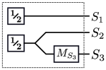
Figure 5. The initial distribution of the CNU from Figure 2 as an MBN.

In an OBN every node $V$ corresponds to a random variable and it represents a probability distribution on $\{0,1\}^{m}$. OBNs are exactly the Bayesian networks considered in [13].

Example 11.

Figure 5 gives an example of a BN where $\nicefrac{{\mathbf{1}}}{{\mathbf{2}}}=\begin{pmatrix}\nicefrac{{1}}{{2}}\\ \nicefrac{{1}}{{2}}\end{pmatrix}$ and $M_{S_{3}}=\begin{pmatrix}\nicefrac{{1}}{{3}}&\nicefrac{{1}}{{2}}\\ \nicefrac{{2}}{{3}}&\nicefrac{{1}}{{2}}\end{pmatrix}$. It encodes exactly the probability distribution from Figure 2. Its term representation is $(g_{1}\otimes(g_{2};\nabla));(\mathrm{id}_{2}\otimes g_{3})$ where $e(g_{1})=e(g_{2})=\nicefrac{{\mathbf{1}}}{{\mathbf{2}}}$ and $e(g_{3})=M_{S_{3}}$.

Definition 12 (MBN semantics).

Let $(B,e)$ be an MBN where the network $B=(V,\ell,s,\mathit{out})$ is of type $n\to m$. The MBN semantics is the matrix $M_{e}(B)$ with

$$\Bigl{(}M_{e}(B)\Bigr{)}(x_{1}\dots x_{m}\mid y_{1}\dots y_{n})=\sum_{\begin{subarray}{c}b\colon W_{B}\to\{0,1\}\\ b(i_{j})=y_{j},b(\textit{out}(o_{i}))=x_{i}\end{subarray}}\quad\prod_{v\in V}\quad e\bigl{(}\ell(v)\bigr{)}\Bigl{(}b(v)\Bigm{|}b(s(v))\Bigr{)}$$

with $x_{1},\dots,x_{m},y_{1},\dots,y_{m}\in\{0,1\}$ where $b$ is applied pointwise to sequences.

Intuitively the function $b$ assigns boolean values to wires, in a way that is consistent with the input/output values ($x_{1}\dots x_{m},y_{1}\dots y_{n}$). For each such assignment, the corresponding entries in the matrices $\ell(v)$ are multiplied. Finally, we sum over all possible assignments.

Remark 3.1.

The semantics $M_{e}(B)$ is compositional. It is the canonical (i.e., free) extension of the evaluation map from single nodes to the causality graph of an MBN $(B,e)$. Here, we rely on two different findings from the literature, namely, the CC-PROP structure of (sub-)stochastic matrices [11] and the characterization of term graphs as the free symmetric monoidal category with graph substition [6]. The formal details can be found in the appendix, see Lemma 18.

4. Updating Bayesian Networks

We have introduced MBNs as a compact and compositional representation of distributions on markings of a CNU. Coming back to the scenario of knowledge update, we now describe how success and failure of operations requested by the observer affect the MBN. We will first describe how the operations can be formulated as matrix operations that tell us which nodes have to be added to the MBN. We shall see that updated MBNs are in general not OBNs, which makes it harder to interpret and retrieve the encoded distribution. However, we shall show that MBNs can efficiently be reduced to OBNs.

Notation: In this section we will use the following notation: first, we will use variants $\mathrm{id}_{n},\nabla_{n},\sigma_{n,m},\top_{n}$ of the operators/matrices $\mathrm{id},\nabla,\sigma,\top$, which have a higher arity (see the definitions in Table 1). Furthermore, we will write $\prod_{i=1}^{k}P_{i}$ for $P_{1}\cdot\ldots\cdot P_{k}$ and $\bigotimes_{i=1}^{k}P_{i}$ for $P_{1}\otimes\cdots\otimes P_{k}$. By $0:1\rightarrow 1$ we denote the $2\times 2$ zero matrix and set $0_{k}=\bigotimes_{i=1}^{k}0$. We also introduce $\mathbf{1}_{b}$ as a notation for the matrix $\begin{pmatrix}1\\ 0\end{pmatrix}$ if $b=1$ (respectively $\begin{pmatrix}0\\ 1\end{pmatrix}$ if $b=0$).

With $\mathrm{diag}(a_{1},\dots,a_{n})$ we denote a square matrix with entries $a_{1},\dots,a_{n}\in[0,1]$ on the diagonal and zero elsewhere. In particular, we will need the sub-stochastic matrices $F_{k,b}:k\to k$ where $F_{k,0}=\mathrm{diag}(\underbrace{1,\dots,1}_{2^{k}-1\text{ times }},0)$ and $F_{k,1}=\mathrm{diag}(0,\underbrace{1,\dots,1}_{2^{k}-1\text{ times }})$.

Given a bit-vector $\mathbf{x}\in\{0,1\}^{n}$, we will write $\mathbf{x}_{[i]}$ respectively $\mathbf{x}_{[i\dots j]}$ to denote the $i$-th entry respectively the sub-sequence from position $i$ to position $j$. If $A\subseteq\{1,\dots,n\}$ we define $\mathbf{x}_{[A]}=\{\mathbf{x}_{[i]}\mid i\in A\}$.

CNU Operations on MBNs

In this section we characterize the operations of Definition 3 as stochastic matrices that can be multiplied with the distribution to perform the update. We describe them as compositions of smaller matrices that can easily be interpreted as changes to an MBN. In the following lemmas, $P:0\rightarrow m$ is always a stochastic matrix representing the distribution of markings of a CNU. Furthermore, $A\subseteq S$ is a set of places and w.l.o.g. we assume that $A=\{1,\dots,k\}$ for some $k\leq m$ (as otherwise we can use permutations that preceed and follow the operations and switch wires as needed).

Starting with the $\mathrm{set}_{A,b}$ operation (3) recall that it is defined in a way so that the marginal distributions of non-affected places $S\backslash A$ stay the same while the marginals of every single place in $A$ report $b\in\{0,1\}$ with probability one. The following lemma shows how the matrix for a set operation can be constructed (see Figure 6).

Lemma 1.

It holds that $\mathrm{set}_{A,b}(P)=\left(\bigotimes_{i=1}^{m}T_{A,b}^{\mathrm{set}}(i)\right)\cdot P$ where $T_{A,b}^{\mathrm{set}}(i)$ is $\mathbf{1}_{b}\cdot\top$ if $i\in A$, and $\mathrm{id}$ otherwise. Moreover, $\bigotimes_{i=1}^{m}T_{A,b}^{\mathrm{set}}(i)$ is stochastic.

Figure 6. String diagrams of the updated distributions after $\mathrm{set}_{A,1}$, $\mathrm{ass}_{A,1}$, $\mathrm{nas}_{A,1}$ operations were applied to an initial distribution $P$.

Next, we deal with the $\mathrm{ass}$ operation. Applying it to a distribution $P$ is simply a conditioning of $P$ on non-emptiness of all places $A$. Intuitively, this means that we keep only entries of $P$ for which the condition is satisfied and set all other entries to zero. However, in order to keep the updated $P$ a probability distribution, we have to renormalize, which already shows that modelling this operation introduces sub-stochastic matrices to the computation. In the next lemma normalization involves the costly computation of a marginal $P_{|A}$ (the probability that all places in $A$ are set to $b$), however omitting the normalization factor will give us a sub-stochastic matrix and we will later show how such sub-stochastic matrices can be removed, in many cases avoiding the full costs of a marginal computation.

Lemma 2.

It holds that $\mathrm{ass}_{A,b}(P)=\frac{1}{P_{|A}}\left(\bigotimes_{i=1}^{m}T_{A,b}^{\mathrm{ass}}(i)\right)\cdot P$ with $P_{|A}=\left(\bigotimes_{i=1}^{m}Q_{A}(i)\right)\cdot P$ where $T_{A,b}^{\mathrm{ass}}(i)$ is $F_{1,1-b}$ if $i\in A$, and $\mathrm{id}$ otherwise. We require that $P_{|A}\neq 0$. Furthermore $Q_{A,b}^{\mathrm{ass}}(i)=\begin{pmatrix}1&0\end{pmatrix}$ if $i\in A$ and $\top$ otherwise.

In contrast to $\mathrm{set}$ and $\mathrm{ass}$, the $\mathrm{nas}$ operation couples all involved places in $A$. Asserting that at least one place has no token means that once the observer learns that e.g. one particular place definitely has a token it affects all the other ones. Thus for updating the distribution we have to pass the wires of places $A$ through another matrix that removes the possibility of all places containing a token and renormalizes.

Lemma 3.

The following characterization holds: $\mathrm{nas}_{A,1}(P)=\frac{1}{P_{|A}^{c}}\left(F_{k,1}\otimes\mathrm{id}_{m-k}\right)\cdot P$ with $P_{|A}^{c}=1-P_{|A}$ ($P_{|A}$ is defined as in Lemma 2). We require that $P_{|A}^{c}\neq 0$.

An analogous result holds for $\mathrm{nas}_{A,0}$ by using $F_{k,0}$.

The previous lemmas determine how to update an MBN $(B,e)$ to incorporate the changes to the encoded distribution stemming from the operations on the CNU. We denote the updated MBN by $(B^{\prime},e^{\prime})$ with $B^{\prime}=(V^{\prime},\ell^{\prime},s^{\prime},\mathrm{out}^{\prime})$.

For the $\mathrm{set}_{A,b}$ operation Lemma 1 shows that we have to add a new node $v_{s}$ and a new generator $g_{s}$ for each $s\in A$. We set $\ell(v_{s})=g_{s}$ and $e^{\prime}(g_{s})=\mathbf{1}_{b}\cdot\top=\begin{pmatrix}1&1\\ 0&0\end{pmatrix}$, $s^{\prime}(v_{s})=\mathrm{out}(o_{s})$ and $\mathrm{out}^{\prime}(o_{s})=v_{s}$. Similarly, this holds for the $\mathrm{ass}$ operation with the only difference that the associated matrix for each $v_{s}$ is $\begin{pmatrix}1&0\\ 0&0\end{pmatrix}$ (cf. Figure 6).

For the $\mathrm{nas}_{A,b}$ operation Lemma 3 defines a usually larger matrix $F_{k,b}:k\to k$ that intuitively couples the random variables for all places in $A$. We cannot simply add a node to the MBN which evaluates to $F_{k,b}$ since nodes in the MBN always have to be of type $n\to 1$. However, one can show (see Lemma 6) that for each $F_{k,b}$-matrix, there exists an MBN $(B^{\prime},e^{\prime})$ such that $M_{e^{\prime}}(B^{\prime})$. This can then be appended to $(B,e)$ which has the same affect as appending a single node with the $F_{k,b}$-matrix.

Simplifying MBNs to OBNs

The characterisations of operations above ensure that updated MBNs correctly evaluate to the updated probability distributions. However, rather than OBNs we obtain MBNs where the complexity of updates is hidden in newly added nodes. Evaluating such MBNs is computationally more expensive because of the additional nodes. Below we show how to simplify the MBN, minimising the number of nodes either after each update or (in a lazy mode) after several updates.

As a first step we provide a lemma that will feature in all following simplifications. It states that every matrix can be expressed by the composition of two matrices.

Lemma 4 (Decomposition of matrices).

Given a matrix $P$ of type $n\to m$ and a set of $k<m$ outputs – without loss of generality we pick $\{m-k+1,\dots,m\}$ – there exist two matrices $P^{\vdash}:n\rightarrow m-k$ and $P^{\dashv}:n+m-k\rightarrow k$ such that

$$(\mathrm{id}_{m-k}\otimes P^{\dashv})\cdot((\nabla_{m-k}\cdot P^{\vdash})\otimes\mathrm{id}_{n})\cdot\nabla_{n}=P,$$ (5)

which is visualized in Figure 7. Moreover, the matrices can be chosen so that $P^{\dashv}$ is stochastic and $P^{\vdash}$ sub-stochastic. If $P$ is stochastic $P^{\vdash}$ can be chosen to be stochastic as well.

We can now deduce the known special case of arc reversal in OBN, stated e.g. in [3].

Figure 7. Schematic string diagram depiction of the decomposition of matrices.

Corollary 5 (Arc reversal in OBNs).

Let $(B,e)$ be an OBN with $B=(V,\ell,s,\mathrm{out})$ and two nodes $u,y\in V$, where $u$ is a direct predecessor of $y$, i.e. $u\in\mathrm{pred}(y)$. Then there exists an OBN $(B^{\prime},e^{\prime})$ with $B^{\prime}=(V,\ell^{\prime},s^{\prime},\mathrm{out})$, evaluating to the same probability distribution, where $\ell^{\prime}(v)=\ell(v)$, $s^{\prime}(v)=s(v)$ if $v\neq u$ and $v\neq y$ and $y\in\mathrm{pred}(u)$. Thus the dependency between $u$ and $v$ is reversed.

Arc reversal comes with a price: as can be seen in the proof, if $u$ is associated with a matrix $P_{u}\colon n\to 1$ and $y$ with a matrix $P_{y}\colon m+1\to 1$, then we have to create new matrices $P^{\prime}_{u}\colon m+n+1\to 1$ and $P^{\prime}_{y}\colon m+n\to 1$, causing new dependencies and increasing the size of the matrix. Hence arc reversal should be used sparingly.

After arc reversal a node might have duplicated inputs, which can be resolved by multiplying the corresponding matrix with $\nabla$, thus reducing the dimension.

Next, we can use Lemma 4 to show that every matrix can be represented as an MBN. This MBN can always be built in a “minimal” way in that only $m$ nodes are needed to represent a $n\to m$ matrix.

Lemma 6.

Let $M:n\rightarrow m$ be a (sub-stochastic) matrix. Then there exists an MBN $(B,e)$ with $B=(V,l,s,\mathrm{out})$ such that $M=M_{e}(B)$, $|V|=m$ and $\mathrm{out}$ is a bijection. Moreover, if $M$ is stochastic we can guarantee that $e(l(v))$ is stochastic for all $v\in V$. If $M$ is sub-stochastic we can guarantee that $v_{\mathit{front}}$ – the first node in a topological ordering of all nodes $V^{\prime}$ – is the only node where $e(l(v))$ is sub-stochastic, all other nodes have stochastic matrices.

Corollary 7.

Let $(B,e)$ be an MBN without inputs and assume that $M_{e}(B)$ is stochastic. Then there exists an OBN $(B^{\prime},e^{\prime})$ such that $M_{e}(B)=M_{e^{\prime}}(B^{\prime})$.

Proof 4.1.

The result follows trivially from the assumptions because for a stochastic MBN without input ports $M_{e}(B)$ is simply a column vector holding a probability distribution. It is well known that every probability distribution can be represented by some (ordinary) Bayesian net. Alternatively the result follows directly from Lemma 6.

We just argued that every MBN can be simplified so that it does not contain any unnecessary nodes and at most one sub-stochastic matrix. However, while Lemma 6 shows that these simplifications are always possible it is not helpful in practice: in fact in the proof we take the full matrix represented by an MBN and then split it into (coupled) single nodes. Since we chose to use MBNs in order not to deal with large distribution vectors in the first place, this approach is not practical. Instead, in the following we will describe methods which allow us to simplify an MBN without computing the matrix first.

First note that MBNs stemming from CNU operations can contain substructures that can locally be replaced by simpler ones. They are depicted in Figure 8.

Figure 8. Equalities on sub-stochastic matrices. Note that (F2) holds only if $P$ is stochastic and for (F4) and (F5) we have to assume $k>1$.

Lemma 8.

The equalities of Figure 8 hold for (sub-)stochastic matrices.

As a result, it makes sense to first eliminate all of these substructures. Then there are two issues left to obtain an OBN. First, there are nodes that lost their direct connection with an output port (since output ports were terminated in a $\mathrm{set}$ operation or since we added an $F_{k,b}$-matrix). Those have to be merged with other nodes. Second, there are sub-stochastic matrices that have to be eliminated as well. The following lemma states that a node not connected to output ports can be merged with its direct successor nodes. This can introduce new dependencies between these successor nodes, but we remove one node from the network.

Lemma 9.

Let $B=(V,\ell,s,\mathrm{out})$ be a causality graph, $e$ an evaluation function such that $(B,e)$ is an MBN. Assume that a node $v_{0}\in V$ is not connected to an output port, i.e. for all $i\in\{1,\dots,m\}:v_{0}\neq\mathrm{out}(o_{i})$, and $e(\ell(v_{0}))$ is stochastic. Then there exists an MBN $(B^{\prime},e^{\prime})$ with $B^{\prime}=(V\backslash\{v_{0}\},\ell^{\prime},s^{\prime},\mathrm{out})$ such that $M_{e}(B)=M_{e^{\prime}}(B^{\prime})$. Moreover, $e^{\prime}\circ\ell^{\prime}|_{\bar{V}}=e\circ\ell|_{\bar{V}}$ and $s^{\prime}|_{\bar{V}}=s|_{\bar{V}}$ where $\bar{V}=V\backslash(\{v_{0}\}\cup\mathrm{succ}(v_{0}))$.

The conditions on $\ell^{\prime}$ and $s^{\prime}$ mean that the update on $B$ is local as it does not affect the whole network. Only the direct successors of $v_{0}$ are affected.

Finally, we have to get rid of sub-stochastic matrices inside the MBN, which have been introduced by the $\mathrm{ass}$ and $\mathrm{nas}$ operations (we assume that we did not normalize yet). The idea is to exchange nodes labelled with sub-stochastic matrices with the predecessor nodes and move them to the front (as in Lemma 6). Once there, normalization is straightforward by normalizing the vectors associated to these nodes.

Lemma 10.

Let $B=(V,\ell,s,\mathrm{out})$ be a causality graph without input ports, i.e. of type $0\to m$, $e$ an evaluation function such that $(B,e)$ is an MBN. Furthermore we require that there is a one-to-one correspondence between output ports and nodes, i.e., $\mathrm{out}$ is a bijection.

Assume that $V^{\prime}\subseteq V$ is the set of all nodes equipped with sub-stochastic matrices, i.e. $e(\ell(v))$ is sub-stochastic for all $v\in V^{\prime}$. Then there exists an OBN $(B^{\prime},e^{\prime})$ with $B^{\prime}=(V,\ell^{\prime},s^{\prime},\mathrm{out})$ such that $M_{e}(B)=M_{e^{\prime}}(B^{\prime})\cdot p_{B}$ where $p_{B}=\top_{m}\cdot M_{e}(B)\leq 1$ is the probability mass of $B$. Moreover, $e^{\prime}\circ\ell^{\prime}|_{\bar{V}}=e\circ\ell|_{\bar{V}}$ and $s^{\prime}|_{\bar{V}}=s|_{\bar{V}}$ where $\bar{V}=V\backslash(V^{\prime}\cup\mathrm{pred}^{*}(V^{\prime}))$.

Note that $\frac{1}{p_{B}}$ (whenever $p_{B}\neq 0$) is the normalization factor that can be obtained by terminating all input ports of $B$. We do not have to compute $p_{B}$ explicitly, but it can be derived from the probabilities of the nodes which have been moved to the front (see proof).

Corollary 11.

Let $B=(V,\ell,s,\mathrm{out})$ be a causality graph without input ports, i.e. of type $0\to m$, $e$ an evaluation function such that $(B,e)$ is an OBN. Let $P=M_{e}(B)$.

Then we can construct OBNs representing $\mathrm{set}_{A,b}(P),\mathrm{ass}_{A,b}(P),\mathrm{nas}_{A,b}(P)$, where

• the $\mathrm{set}$ operation modifies only $\{\mathrm{out}(o_{i})\mid i\in A\}$ and their direct successors and

• the $\mathrm{ass}$ and $\mathrm{nas}$ operations modify only $\{\mathrm{out}(o_{i})\mid i\in A\}$ and their predecessors.

The operations are costly whenever a node has many predecessors or direct successors. In a certain way this is unavoidable because our operations are related to the computation of marginals, which is $\mathsf{NP}$-hard [5]. However, if the Bayesian network has a comparatively “flat” structure, we expect that the efficiency is rather high in the average case, as supported by our runtime results below. Applying the $\mathrm{nas}$ operation will introduce dependencies for the random variables corresponding to the pre- and post-conditions of a transition, however this effect is localized if we consider particular classes of Petri nets, such as free-choice nets [8].

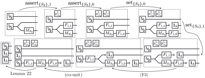
Figure 9. Exemplary update process for the $\mathrm{success}_{t_{4}}$ operation of our running CNU example. Here $\nicefrac{{\mathbf{1}}}{{\mathbf{2}}}=\begin{pmatrix}\nicefrac{{1}}{{2}}\\ \nicefrac{{1}}{{2}}\end{pmatrix}$ and $M_{S_{3}}=\begin{pmatrix}\nicefrac{{1}}{{3}}&\nicefrac{{1}}{{2}}\\ \nicefrac{{2}}{{3}}&\nicefrac{{1}}{{2}}\end{pmatrix}$.

Example 11.

Figure 9 shows an update process, following a lazy evaluation strategy, for a Bayesian net representing the probability distribution from Figure 2.

5. Implementation

In order to quantitatively assess the performance of MBNs we developed a prototypical C++ implementation of the concepts in this paper, allowing to read, write, simplify, generate, and visualize MBNs as well as perform operations on CNUs that update an underlying MBN. The implementation is open-source and freely available on GitHub.

As a first means of obtaining runtime results we randomly generated CNs with a range of different parameters: e.g. number of places, number of places in a precondition of a transition, places in the initial marking etc. We then successively picked transitions at random to fire and performed the necessary operations to update the MBN and simplify it to an OBN.

We chose to guarantee a success rate of transition firing of around $1/3$. We argue that given the fact that we model an observer with prior knowledge it is realistic to assume a certain rate of successful transitions. A very low sucess rate leads to an accumulation of successive $F_{k,b}$ matrices which can only be eliminated using the costly operations on substochastic matrices (see proof of Lemma 10). One could implement effective simplification strategies merging successive $F_{k,b}$ matrices – since composing 0,1 diagonal matrices yields again 0,1 diagonal matrices. However, this is out of scope of this publication.

The plot on the left of Figure 10 shows a comparison between run times when performing CNU operations directly on the joint distribution versus our MBN implementation. One can clearly observe the exponential increase when using the joint distribution while the MBN implementation in this setup stays relatively constant. The plot on the right of Figure 10 hints towards an increase in complexity when CNs – and thus MBNs – are more coupled. When increasing the maximum number of places in the precondition of a transition we observe an increase in run times. The number of outliers with a dramatic increase in run times seem to rise as well.

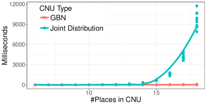
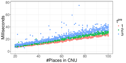
Figure 10. Averaged runtimes for performing 100 CNU operations using joint distributions or MBNs.

6. Conclusion

Related work: A concept similar to our nets with uncertainty has been proposed in [17], but without any mechanism for efficiently representing and updating the probability distribution. There are also links to Hidden Markov Models [24] for inferring probabilistic knowledge on hidden states by observing a model.

Bayesian networks were introduced by Pearl in [21] to graphically represent random variables and their dependencies. Our work has some similarities to his probabilistic calculus of actions (do-calculus) [22] which supports the empirical measurement of interventions. However, while Pearl’s causal networks model describe true causal relationships, in our case Bayesian networks are just compact symbolic representations of huge probability distributions. There is also a notion of dynamic Bayesian networks [20], where a random variable has a separate instance for each time slice. We instead keep only one instance of every random variable, but update the BN itself. There is substantial work on updating Bayesian networks (for instance [14]) with the orthogonal aim of learning BNs from training data.

PROPs have been introduced in [19], foundations for term-based proofs have been studied in [18] and their graphical language has been developed in [26, 4]. Bayesian networks as PROPs have already been studied in [11] under the name of causal theories, as well as in [16, 15] in order to give a predicate/state transformer semantics to Bayesian networks. However, these papers do not explicitly represent the underlying graph structure and in particular they do not consider updates of Bayesian networks.

We use the results from [6] in order to show that our causality graphs are in fact term graphs, which are freely generated gs-monoidal categories, which in turn are CC-structured PROPs. Although this result is intuitive, it is non-trivial to show: given two terms with isomorphic underlying graphs, each can be reduced to a normal form which can be converted into each other using the axioms of a CC-structured PROP. Similar results are given in [10, 2] for PROPs with multiplication and unit, in addition to comultiplication and counit.

Future work: We would like to investigate further operations on probability distributions, however it is unclear whether every operation can be efficiently implemented. For instance linear combinations of probability distributions seem difficult to handle.

Van der Aalst [28] showed that all reachable markings in certain free-choice nets can be inferred from their enabled transitions. An unrestricted observer may therefore be in a very strong position. Privacy research often considers statistical queries, such as how many records with certain properties exist in the database [9, 7]. To model such weaker queries we require labelled nets where instead of transitions we observe their labels. To implement this in BNs requires a disjunction of the enabledness conditions of all transitions with the same label. Furthermore we are interested in scenarios where certain transitions are unobservable.

Appendix A Proofs

See 4

Proof A.1.

For the case of $\mathrm{fail}^{\mathit{pre}}$ and $\mathrm{fail}^{\mathit{post}}$ the equation is a straightforward reformulation of the definition. For $\mathrm{success}$ we have:

$$= \sum_{m^{\prime}\Rightarrow^{t}m}\mathrm{ass}_{{t}^{\bullet},0}(\mathrm{ass}_{\prescript{\bullet}{}{t},1}(p)(m^{\prime}))=\sum_{m=\bar{m}\cup{t}^{\bullet}}\sum_{\bar{m}=m^{\prime}\backslash\prescript{\bullet}{}{t}}\mathrm{ass}_{{t}^{\bullet},0}(\mathrm{ass}_{\prescript{\bullet}{}{t},1}(p)(m^{\prime}))$$

$$= \sum_{m=\bar{m}\cup{t}^{\bullet}}\mathrm{set}_{\prescript{\bullet}{}{t},0}(\mathrm{ass}_{{t}^{\bullet},0}(\mathrm{ass}_{\prescript{\bullet}{}{t},1}(p)))(\bar{m})$$

$$= \mathrm{set}_{{t}^{\bullet},1}(\mathrm{set}_{\prescript{\bullet}{}{t},0}(\mathrm{ass}_{{t}^{\bullet},0}(\mathrm{ass}_{\prescript{\bullet}{}{t},1}(p))))(m)=\mathrm{success}_{t}(p)(m)$$

See 9

Proof A.2 (Proof sketch).

Let $V_{1}=\mathrm{pred}^{*}(V^{\prime})$ be the set of all predecessor nodes of $V^{\prime}$ and let $V_{3}$ be the set of remaining nodes. Furthermore let $k=n+|V_{1}|$. Since $V^{\prime}$ is path-closed we can construct a CG $B_{2}$ that contains exactly the nodes in $V^{\prime}$ and has as input ports exactly those ports needed by these nodes and one output port for every element in $V^{\prime}$.

Then we can construct a CG that contains all nodes of $V_{1}$ and whose output ports link to all input ports as well as all nodes in $V_{1}$. We then duplicate those wires that are needed by $B_{2}$ and permute them to the end of the output port sequence. This gives us the CG $B_{1}$.

Finally, $B_{3}$ contains all nodes of $V_{3}$: due to the wiring it can access all input ports as well as all nodes of $V_{1}$ and $V_{2}$. At the very end all wires are terminated, duplicated and/or permuted as required by $B$.

Lemma 18.

For each MBN $(B,e)$, $M_{e}(B)$ is the value of the free extension of $e$ to CGs from Proposition 8 applied to the isomorphism class of $B$ using that it is actually the free CC-PROP as it is the free GS-monoidal category [6].

Proof A.3.

It is sufficient to show that $M_{e}$ is functorial, in particular it respects composition and tensor, as well as identity, $\nabla$, $\sigma$ and $\top$. We only consider the following two cases, the rest is analogous.

 

For instance, let two MBNs $B_{i}=(V_{i},\ell_{i},s_{i},\mathit{out}_{i})$, $i\in\{1,2\}$, with $B_{1}\colon n\to m$, $B_{2}\colon m\to\ell$ be given. We set $B=B_{1};B_{2}$. We apply $M_{e}$ to $B$ and obtain for $\mathbf{x}\in\{0,1\}^{\ell}$, $\mathbf{z}\in\{0,1\}^{m}$:

$$\bigg{(}M_{e}(B_{2})\cdot M_{e}(B_{1})\bigg{)}(\mathbf{x},\mathbf{z})$$

$$= \sum_{\mathbf{y}\in\{0,1\}^{m}}M_{e}(B_{2})(\mathbf{x},\mathbf{y})\cdot M_{e}(B_{2})(\mathbf{y},\mathbf{z})$$

$$= \sum_{\mathbf{y}\in\{0,1\}^{m}}\bigg{(}\sum_{\begin{subarray}{c}b_{2}\colon W_{B_{2}}\to\{0,1\}\\ b_{2}(i_{j})=y_{j}\\ b_{2}(\textit{out}_{2}(o_{i}))=x_{i}\end{subarray}}\quad\prod_{v\in V_{2}}\quad e(\ell_{2}(v))(b_{2}(v)\mid b_{2}(s_{2}(v)))\bigg{)}\cdot$$

$$\qquad\qquad\bigg{(}\sum_{\begin{subarray}{c}b_{1}\colon W_{B_{1}}\to\{0,1\}\\ b_{1}(i_{j})=z_{j}\\ b_{1}(\textit{out}_{1}(o_{i}))=y_{i}\end{subarray}}\quad\prod_{v\in V_{1}}\quad e(\ell_{1}(v))(b_{1}(v)\mid b_{1}(s_{1}(v)))\bigg{)}$$

$$= \sum_{\mathbf{y}\in\{0,1\}^{m}}\sum_{\begin{subarray}{c}b_{2}\colon W_{B_{2}}\to\{0,1\}\\ b_{2}(i_{j})=y_{j}\\ b_{2}(\textit{out}_{2}(o_{i}))=x_{i}\end{subarray}}\quad\sum_{\begin{subarray}{c}b_{1}\colon W_{B_{1}}\to\{0,1\}\\ b_{1}(i_{j})=z_{j}\\ b_{1}(\textit{out}_{1}(o_{i}))=y_{i}\end{subarray}}$$

$$\qquad\qquad\prod_{v\in V_{2}}\quad\prod_{v\in V_{1}}\quad\bigg{(}e(\ell_{2}(v))(b_{2}(v)\mid b_{2}(s_{2}(v)))\cdot e(\ell_{1}(v))(b_{1}(v)\mid b_{1}(s_{1}(v)))\bigg{)}$$

$$= \sum_{\begin{subarray}{c}b\colon W_{B}\to\{0,1\}\\ b(i_{j})=z_{j}\\ b(\textit{out}(o_{i}))=x_{i}\end{subarray}}\qquad\prod_{v\in V}\quad e(\ell(v))(b(v)\mid b(s(v)))$$

$$= M_{e}(B)=M_{e}(B_{1};B_{2})$$

We assume that $\mathbf{x}=x_{1}\dots x_{\ell}$, $\mathbf{y}=y_{1}\dots y_{m}$, $\mathbf{z}=z_{1}\dots z_{n}$.

Note that the equality sign on the second last line is due to the fact that assignments $b_{1}\colon W_{B_{1}}\to\{0,1\},b_{2}\colon W_{B_{2}}\to\{0,1\}$ of boolean values to wires can be merged into one assignment $b\colon W_{B}\to\{0,1\}$ on $B$ whenever they agree on the interface, i.e., whenever $b_{1}(\mathit{out}_{1}(o_{k}))=y_{k}=b_{2}(i_{k})$.

 

Next we check that $M_{e}(\sigma)=\sigma$. (Here we use some overloading: $\sigma$ stands for a CG as well as for a stochastic matrix.) The MBN $\sigma$ is of the form $(V,\ell,s,\mathit{out})=(\emptyset,[\,],[\,],[o_{1}\mapsto i_{2},o_{2}\mapsto i_{1}])\colon 2\to 2$.

Let $x_{1},x_{2},y_{1},y_{2}\in\{0,1\}$. We compute

$$M_{e}(\sigma)(x_{1}x_{2},y_{1}y_{2})=\sum_{\begin{subarray}{c}b\colon W_{\sigma}\to\{0,1\}\\ b(i_{j})=y_{j}\\ b(\textit{out}(o_{i}))=x_{i}\end{subarray}}\qquad\prod_{v\in V}\quad e(\ell(v))(b(v)\mid b(s(v)))$$

In this case the product is always empty, evaluating to a value of $1$. The sum is non-empty whenever an assignment $b$ exists, i.e., if $y_{1}=b(i_{1})=b(\mathit{out}(o_{2}))=x_{2}$ and $y_{2}=b(i_{2})=b(\mathit{out}(o_{1}))=x_{1}$. In these cases, $M_{e}(\sigma)(x_{1}x_{2},y_{1}y_{2})=1$, otherwise the sum is empty and $M_{e}(\sigma)(x_{1}x_{2},y_{1}y_{2})=0$. Combined, we obtain $M_{e}(\sigma)=\sigma$.

See 1

Proof A.4.

First consider the special case of a singleton $A=\{1\}$ and $b=1$. (The case for $b=0$ is analogous.) We compute

$$M:=\bigotimes_{i=1}^{m}T_{\{1\},1}^{\mathrm{set}}(i)=\begin{pmatrix}1&1\\ 0&0\end{pmatrix}\otimes\bigotimes_{i=2}^{m}\mathrm{id}=\begin{pmatrix}1&1\\ 0&0\end{pmatrix}\otimes\mathrm{id}_{m-1}=\begin{pmatrix}\mathrm{id}_{m-1}&\mathrm{id}_{m-1}\\ 0_{m-1}&0_{m-1}\end{pmatrix}.$$

Thus, whenever $\mathbf{x}\in\{0,1\}^{m}$:

$$(M\cdot P)(\mathbf{x})=\begin{cases}P(1\mathbf{x}_{[2\dots m]})+P(0\mathbf{x}_{[2\dots m]})&\text{ if }\mathbf{x}_{[1]}=1\\ 0&\text{ if }\mathbf{x}_{[1]}=0\end{cases}\quad=\mathrm{set}_{\{1\},1}(P).$$

The general case follows by using $\mathrm{set}_{A,b}=\mathrm{set}_{\{s_{k}\},b}\circ\dots\circ\mathrm{set}_{\{s_{1}\},b}$ where $A=\{s_{1},\dots,s_{k}\}$ and the fact that because the stochastic matrices form a PROP (see the first law (mixing of composition and tensor) in Table 1), we have $\bigotimes_{i=1}^{m}T_{A,b}^{\mathrm{set}}(i)=\prod_{l=1}^{k}(\bigotimes_{i=1}^{m}T_{\{s_{l}\},b}^{\mathrm{set}}(i))$. Moreover, $\bigotimes_{i=1}^{m}T_{A,b}^{\mathrm{set}}(i)$ is a stochastic matrix because all $T_{A,b}^{\mathrm{set}}(i)$ are stochastic and the tensor preserves this property.

See 2

Proof A.5.

Again we first consider the singleton case $A=\{1\}$ and $b=1$. (The case for $b=0$ is analogous.) Then

$$M:=\bigotimes_{i=1}^{m}T_{\{1\},1}^{\mathrm{ass}}(i)=\begin{pmatrix}1&0\\ 0&0\end{pmatrix}\otimes\mathrm{id}_{m-1}=\begin{pmatrix}\mathrm{id}_{m-1}&0_{m-1}\\ 0_{m-1}&0_{m-1}\end{pmatrix},$$

and thus $(M\cdot P)(\mathbf{x})=\begin{cases}P(\mathbf{x})&\text{ if }\mathbf{x}_{[1]}=1\\ 0&\text{ if }\mathbf{x}_{[1]}=0\end{cases}$

Also $\left(\bigotimes_{i=1}^{m}Q_{A}(i)\right)(\mathbf{x})=\begin{cases}1&\text{ if }\mathbf{x}_{[A]}=\{1\}\\ 0&\text{ otherwise }\end{cases}$

As a result, $P_{|A}=\sum_{\mathbf{x}|\mathbf{x}_{[A]}=\{1\}}P(\mathbf{x})$ and thus $\frac{1}{P_{|A}}(M\cdot P)=\mathrm{ass}_{A,1}(P)$. $M$ is not stochastic because clearly the last $m-1$ columns add up to $0$.

Similarly to the $\mathrm{set}$ case we have $\mathrm{ass}_{A,b}=\mathrm{ass}_{\{s_{k}\},b}\circ\dots\circ\mathrm{ass}_{\{s_{1}\},b}$ where $A=\{s_{1},\dots,s_{k}\}$ and $\bigotimes_{i=1}^{m}T_{A,b}^{\mathrm{ass}}(i)=\prod_{l=1}^{k}(\bigotimes_{i=1}^{m}T_{\{s_{l}\},b}^{\mathrm{ass}}(i))$.

See 3

Proof A.6.

We have $M:=\left(F_{k,1}\otimes\mathrm{id}_{m-k}\right)=\begin{pmatrix}0_{m-k}&0\\ 0&\mathrm{id}_{k}\end{pmatrix}$. This means that when multiplying we get $(M\cdot P)(\mathbf{x})=\begin{cases}0&\text{ if }\mathbf{x}_{A}=\{1\}\\ P(\mathbf{x})&\text{ otherwise }\end{cases}$.

As shown in the $\mathrm{ass}$ case $P_{|A}=\sum_{\mathbf{x}|\mathbf{x}_{[A]}=\{1\}}P(\mathbf{x})$ and thus $P_{|A}^{c}=1-P_{|A}=\sum_{\mathbf{x}|\mathbf{x}_{[A]}\not=1}P(\mathbf{x})$ and together we get $\mathrm{nas}_{A,1}(P)=\frac{1}{P_{|A}^{c}}(M\cdot P)$.

See 4

Proof A.7.

In the following we denote by $\mathbf{z}\in\{0,1\}^{n}$, $\mathbf{x}\in\{0,1\}^{m-k}$ and $\mathbf{y}\in\{0,1\}^{k}$ bit vectors that represent the inputs of $P$ (for $\mathbf{z}$), outputs of $P^{\vdash}$ (for $\mathbf{x}$) respectively the outputs of $P^{\dashv}$ (for $\mathbf{y}$). We now define

$$P^{\vdash}(\mathbf{x}\mid\mathbf{z})=\sum_{\mathbf{v}\in\{0,1\}^{k}}P(\mathbf{x}\mathbf{v}\mid\mathbf{z})\quad\text{ and }\quad P^{\dashv}(\mathbf{y}\mid\mathbf{x}\mathbf{z})=\frac{P(\mathbf{x}\mathbf{y}\mid\mathbf{z})}{\sum_{\mathbf{v}\in\{0,1\}^{k}}P(\mathbf{x}\mathbf{v}\mid\mathbf{z})}=\frac{P(\mathbf{x}\mathbf{y}\mid\mathbf{z})}{P^{\vdash}(\mathbf{x}\mid\mathbf{z})}$$

Whenever $P^{\vdash}(\mathbf{x}\mid\mathbf{z})=\sum_{\mathbf{v}\in\{0,1\}^{k}}P(\mathbf{x}\mathbf{v}\mid\mathbf{z})=0$ it holds that $P(\mathbf{x}\mathbf{v}\mid\mathbf{z})=0$ for every $\mathbf{v}\in\{0,1\}^{k}$. In this case the row of $P^{\dashv}$ corresponding to $\mathbf{x}\mathbf{z}$ can be chosen arbitrarily, as long as it adds up to $1$. We observe that $P^{\dashv}$ is stochastic because $\sum_{\mathbf{y}_{1}\in\{0,1\}^{k}}P^{\dashv}(\mathbf{y}_{1}|\mathbf{x}\mathbf{z})=1$ for all $\mathbf{x}$, $\mathbf{z}$. $P^{\vdash}$ on the other hand is by definition stochastic if and only if $P$ is stochastic: If we keep the column index ($\mathbf{x}$ in the case of $P^{\vdash}$ and $\mathbf{x}\mathbf{y}$ in the case of $P^{\dashv}$) fixed and sum over the row index, we straightforwardly obtain $1$ in both cases.

To use the more intuitive matrix notation one could equivalently define $P^{\vdash}=(\mathrm{id}_{k}\otimes\top_{m-k})\cdot P$. However, such a simple characterization in terms of matrix compositions does not exist for $P^{\dashv}$.

Finally, we can check that $P^{\vdash}$ and $P^{\dashv}$ satisfy (6).

$$((\mathrm{id}_{m-k}\otimes P^{\dashv})\cdot((\nabla_{m-k}\cdot P^{\vdash})\otimes\mathrm{id}_{n})\cdot\nabla_{n})(\mathbf{x}\mathbf{y}\mid\mathbf{z})$$

$$=((\mathrm{id}_{m-k}\otimes P^{\dashv})\cdot((\nabla_{m-k}\cdot P^{\vdash})\otimes\mathrm{id}_{n}))(\mathbf{x}\mathbf{y}\mid\mathbf{z}\mathbf{z})$$

$$=\sum_{\mathbf{x}_{1},\mathbf{x}_{2}\in\{0,1\}^{m-k},\mathbf{z}_{1}\in\{0,1\}^{n}}(\mathrm{id}_{m-k}\otimes P^{\dashv})\left(\mathbf{x}\mathbf{y}\mid\mathbf{x}_{1}\mathbf{x}_{2}\mathbf{z}_{1}\right)\cdot((\nabla_{m-k}\cdot P^{\vdash})\otimes\mathrm{id}_{n})(\mathbf{x}_{1}\mathbf{x}_{2}\mathbf{z}_{1}\mid\mathbf{z}\mathbf{z})$$

$$=\sum_{\mathbf{x}_{1},\mathbf{x}_{2}\in\{0,1\}^{m-k},\mathbf{z}_{1}\in\{0,1\}^{n}}\mathrm{id}_{m-k}(\mathbf{x}\mid\mathbf{x}_{1})\cdot P^{\dashv}(\mathbf{y}\mid\mathbf{x}_{2}\mathbf{z}_{1})\cdot(\nabla_{m-k}\cdot P^{\vdash})(\mathbf{x}_{1}\mathbf{x}_{2}\mid\mathbf{z})\cdot\mathrm{id}_{n}(\mathbf{z}_{1}\mid\mathbf{z})$$

$$=\sum_{\mathbf{x}_{2}\in\{0,1\}^{m-k}}P^{\dashv}(\mathbf{y}\mid\mathbf{x}_{2}\mathbf{z})\cdot(\nabla_{m-k}\cdot P^{\vdash})(\mathbf{x}\mathbf{x}_{2}\mid\mathbf{z})$$

$$=\sum_{\mathbf{x}_{2}\in\{0,1\}^{m-k}}P^{\dashv}(\mathbf{y}\mid\mathbf{x}_{2}\mathbf{z})\cdot\bigg{(}\sum_{\mathbf{x}_{3}\in\{0,1\}^{m-k}}\nabla_{m-k}(\mathbf{x}\mathbf{x}_{2}\mid\mathbf{x}_{3})\cdot P^{\vdash}(\mathbf{x}_{3}\mid\mathbf{z})\bigg{)}$$

$$=P^{\dashv}(\mathbf{y}\mid\mathbf{x}\mathbf{z})\cdot P^{\vdash}(\mathbf{x}\mid\mathbf{z})$$

$$=P(\mathbf{x}\mathbf{y}\mid\mathbf{z})$$

where we used that $\mathrm{id}_{i}(\mathbf{y}\mid\mathbf{x})$ is non-zero only when $\mathbf{y}=\mathbf{x}$ and that $\nabla_{i}(\mathbf{y}_{1}\mathbf{y}_{2}\mid\mathbf{x})$ is non-zero iff $\mathbf{y}_{1}=\mathbf{y}_{2}=\mathbf{x}$.

Whenever $P^{\vdash}(\mathbf{x}\mid\mathbf{z})=0$ the product in the second-last line is $0$. As argued above in this case $P(\mathbf{x}\mathbf{y}\mid\mathbf{z})=0$ as well and the last equality holds.

See 5

Proof A.8.

Let $g_{u}=\ell(u)$, $g_{y}=\ell(y)$ and $e(g_{u})=P_{u}$, $e(g_{y})=P_{y}$.

We assume without loss of generality that $s(y)=\mathbf{u}u$, otherwise we have to rearrange the inputs of $y$. Let $m=|\mathbf{u}|$ and $n=|s(u)|$.

Since the set $\{u,y\}$ is closed with respect to paths, we can use Lemma 9 and represent $B$ by the following term: $t_{1};(\mathrm{id}_{k}\otimes(\underbrace{(\mathrm{id}_{m}\otimes(B_{g_{u}};\nabla));(B_{g_{y}}\otimes\mathrm{id})}_{t_{uy}}));t_{3}$. The term $t_{uy}$ corresponds to the matrix $M_{e}(t_{uy})=P=(\mathrm{id}\otimes P_{y})\cdot((\nabla\cdot P_{u})\otimes\mathrm{id}_{m})$, which is a matrix of type $m+n\to 2$. We now apply Lemma 4 to $P$ for $k=1$ and obtain matrices $P^{\prime}_{y}\colon m+n\to 1$, $P^{\prime}_{u}\colon m+n+1\to 1$ with $(\mathrm{id}\otimes P^{\prime}_{u})\cdot((\nabla\cdot P^{\prime}_{y})\otimes\mathrm{id}_{m})\cdot\nabla_{m}=P$. We transform this into a term $t_{y}=\nabla_{m};((B_{g^{\prime}_{y}};\nabla)\otimes\mathrm{id}_{m});(\mathrm{id}\otimes B_{g^{\prime}_{u}})$ where $g^{\prime}_{y},g^{\prime}_{u}$ are two new generators, evaluating to $P^{\prime}_{u}$, $P^{\prime}_{y}$.

If we replace $t_{uy}$ in the term above by $t_{yu}$ we obtain a new BN where the order of $u,y$ is reversed and the other structure remains unchanged.

See 6

Proof A.9.

The statement is a direct result of Lemma 4. Using $k=1$ we get from Lemma 4 $M_{m-1}=M^{\vdash}:n\rightarrow m-1$ and $M^{(m-1)}=M^{\dashv}:n+1\rightarrow 1$ such that

$$(\mathrm{id}\otimes M_{m-1})\cdot((\nabla\cdot M^{(m-1)})\otimes\mathrm{id}_{n})\cdot\nabla_{n}=M.$$ (6)

We can now apply Lemma 4 again to $M_{m-1}$ to get a new $M_{m-2}$ and $M^{(m-2)}$. Doing this process recursively in step $i$ we end up with smaller and smaller matrices $M_{m-i}:n\rightarrow m-1$ and $M^{(m-i)}:n+1\rightarrow 1$. After a total of $m-1$ steps we end up with $M_{1}:n\rightarrow 1$ and we stop. The matrices $M_{1},M^{(2)},\dots,M^{(m-1)}$ all have type $n+1\rightarrow 1$. Moreover, Lemma 4 guarantees that $M^{(2)},\dots,M^{(m-1)}$ can always be chosen to be stochastic matrices. $M_{1}$ can be chosen stochastic if and only if $M$ is stochastic. For $B$ we now set $V=\{v_{1},\dots,v_{m}\}$, $l(v_{j})=g_{j}$ for all $j=1,\dots,m$ and $s(v_{j})=(v_{j-1},i_{1},\dots,i_{n})$ for $j=2,\dots,m$ and $s(v_{1})=(i_{1},\dots,i_{n})$ and $\mathrm{out}(o_{j})=v_{j}$ for $j=1,\dots,m$. Accordingly we set $e(g_{j})=M^{(j)}$ for $j=2,\dots,m$ and $e(g_{1})=M_{1}$. It is easy to verify that $(B,e)$ now forms an MBN.

See 8

Proof A.10.

In the following we assume $b=1$. The case $b=0$ is always analogous. To show (F1) we compute

$$\nabla\cdot\begin{pmatrix}1\\ 0\end{pmatrix}=\begin{pmatrix}1\\ 0\\ 0\\ 0\end{pmatrix}=\begin{pmatrix}1\\ 0\end{pmatrix}\otimes\begin{pmatrix}1\\ 0\end{pmatrix}.$$

For (F2) let $P:k\to 1$ be a stochastic matrix. Then

$$\top\cdot P=\begin{pmatrix}1&1\end{pmatrix}\cdot\begin{pmatrix}p_{1}&\cdots&p_{2^{k}}\\ \bar{p}_{1}&\cdots&\bar{p}_{2^{k}}\end{pmatrix}=\underbrace{\begin{pmatrix}1&\cdots&1\end{pmatrix}}_{2^{k}\text{ times }}=\top_{k}.$$

For (F4) we calculate

$$F_{k,1}\cdot(\begin{pmatrix}1\\ 0\end{pmatrix}\otimes\mathrm{id}_{k-1,1})=F_{k,1}\cdot\begin{pmatrix}\mathrm{id}_{k-1}\\ 0_{k-1}\end{pmatrix}=\begin{pmatrix}F_{k-1,1}\\ 0_{k-1}\end{pmatrix}=\begin{pmatrix}1\\ 0\end{pmatrix}\otimes F_{k-1,1}.$$

To show (F5) we calculate

$$F_{k,1}\cdot(\begin{pmatrix}0\\ 1\end{pmatrix}\otimes\mathrm{id}_{k-1})=F_{k,1}\cdot\begin{pmatrix}0_{k-1}\\ \mathrm{id}_{k-1}\end{pmatrix}=\begin{pmatrix}0_{k-1}\\ \mathrm{id}_{k-1}\end{pmatrix}=\begin{pmatrix}0\\ 1\end{pmatrix}\otimes\mathrm{id}_{k-1}.$$

In order to prove equality (F3) we have to show

$$(F_{k,1}\otimes\mathrm{id})\cdot(\mathrm{id}_{k-1}\otimes\nabla)=(\mathrm{id}_{k-1}\otimes\nabla)\cdot F_{k,1}.$$

Given $\mathbf{x},\mathbf{y}\in\{0,1\}^{k}$ it holds that $F_{k,1}(\mathbf{x},\mathbf{y})=1$ iff $\mathbf{x}=\mathbf{y}$ and $\mathbf{x},\mathbf{y}\neq 1\ldots 1$. Otherwise $F_{k,1}(\mathbf{x},\mathbf{y})=0$.

Now, given $\mathbf{z}\mathrm{z}\in\{0,1\}^{k+1},\mathbf{x}\in\{0,1\}^{k}$, we have

$$((F_{k,1}\otimes\mathrm{id})\cdot(\mathrm{id}_{k-1}\otimes\nabla))(\mathbf{z}\mathrm{z}\mid\mathbf{x})$$

$$= \sum_{\mathbf{y}\mathrm{y}\in\{0,1\}^{k+1}}(F_{k,1}\otimes\mathrm{id})(\mathbf{z}\mathrm{z}\mid\mathbf{y}\mathrm{y})\cdot(\mathrm{id}_{k-1}\otimes\nabla)(\mathbf{y}\mathrm{y}\mid\mathbf{x})$$

$$= \sum_{\mathbf{y}\mathrm{y}\in\{0,1\}^{k+1}}F_{k,1}(\mathbf{z}\mid\mathbf{y})\cdot[\mathrm{z}=\mathrm{y}]\cdot[\mathbf{x}=\mathbf{y}]\cdot[\mathrm{y}=\mathbf{y}_{[k]}=\mathbf{x}_{[k]}]$$

$$= \left\{\begin{array}[]{ll}F_{k,1}(\mathbf{z}\mid\mathbf{x})&\text{if $\mathbf{x}_{[k]}=\mathrm{z}$}\\ 0&\text{otherwise}\end{array}\right\}=\left\{\begin{array}[]{ll}1&\text{if $\mathbf{z}=\mathbf{x}$, $\mathbf{x},\mathbf{z}\neq 1\ldots 1$, $\mathbf{x}_{[k]}=\mathrm{z}$}\\ 0&\text{otherwise}\end{array}\right.$$

Note that $[\mathbf{x}=\mathbf{y}]$ stands for $1$ if the equality holds and for zero otherwise.

Furthermore:

$$((\mathrm{id}_{k-1}\otimes\nabla)\cdot F_{k,1})(\mathbf{z}\mathrm{z}\mid\mathbf{x})$$

$$= \sum_{\mathbf{y}\in\{0,1\}^{k}}(\mathrm{id}_{k-1}\otimes\nabla)(\mathbf{z}\mathrm{z}\mid\mathbf{y})\cdot F_{k,1}(\mathbf{y}\mid\mathbf{x})$$

$$= \sum_{\mathbf{y}\in\{0,1\}^{k}}[\mathbf{z}=\mathbf{y}]\cdot[\mathrm{z}=\mathbf{z}_{[k]}=\mathbf{y}_{[k]}]\cdot F_{k,1}(\mathbf{y}\mid\mathbf{x})$$

$$= \left\{\begin{array}[]{ll}F_{k,1}(\mathbf{z}\mid\mathbf{x})&\text{if $\mathbf{z}_{[k]}=\mathrm{z}$}\\ 0&\text{otherwise}\end{array}\right\}=\left\{\begin{array}[]{ll}1&\text{if $\mathbf{z}=\mathbf{x}$, $\mathbf{x},\mathbf{z}\neq 1\ldots 1$, $\mathbf{z}_{[k]}=\mathrm{z}$}\\ 0&\text{otherwise}\end{array}\right.$$

And it is easy to see that both end results are equal.

See 9

Proof A.11.

We set $V^{\prime}=\mathrm{succ}(v_{0})$ and fix a topological ordering on $V^{\prime}$. Then we successively exchange $v_{0}$ with the next successor in the topological ordering, using arc reversal as described in Corollary 5. Note that in arc reversal the number of successors of $v_{0}$ decreases by one and the matrix associated to $v_{0}$ will remain stochastic (see Lemma 4), hence at some point $v_{0}$ will have no successors and we can use equality (F2) from Figure 8 in order to eliminate it.

Note that only the source and labelling functions of the direct successors of $v_{0}$ are affected and the respective functions remain unchanged for the nodes in $\bar{V}$.

See 10

Proof A.12.

We iterate over $V^{\prime}$ and by using again Lemma 6 we can replace the sub-MBN induced by $v_{0}\in V^{\prime}$ and its predecessors by one that has a single sub-stochastic matrix in the front, without predecessors. Doing this iteratively, we can move every sub-stochastic matrix to the front of the MBN where they do not have any predecessors. This results in an MBN $(B^{\prime},\hat{e})$. Only the nodes in $V^{\prime}$ and their predecessor nodes, but not the other nodes are affected, that is $e^{\prime}\circ\ell^{\prime}|_{\bar{V}}=e\circ\ell|_{\bar{V}}$ and $s^{\prime}|_{\bar{V}}=s|_{\bar{V}}$.

Through normalization we can then get rid of the sub-stochasticity for every node: assume that $\hat{V}$ contains the nodes in $B^{\prime}$ equipped with sub-stochastic matrices. We terminate all output ports of $B^{\prime}$ by computing $\top_{m}\cdot M_{\hat{e}}(B^{\prime})=\top_{m}\cdot M_{e}(B)=p_{B}$, since $B,B^{\prime}$ specify the same matrix. Due to equality (F2) in Figure 8 this means that all stochastic nodes disappear, only the sub-stochastic nodes remain and hence $p_{B}=\prod_{v\in\hat{V}}(Q_{v}(0)+Q_{v}(1))$ where $Q_{v}=\hat{e}(\ell^{\prime}(v))$. Note that $Q_{v}$ is simply a column vector with two entries. The value $q_{v}=Q_{v}(0)+Q_{v}(1)$ results when a sub-stochastic node without predecessors is terminated. We now replace each $Q_{v}$ by $\frac{1}{q_{v}}Q_{v}$, which is a stochastic matrix, resulting in a new evaluation function $e^{\prime}$. Looking at the definition of $M_{e}$ in Section 2, we observe that the values $\frac{1}{q_{v}}$ can be factored out and hence:

$$M_{e^{\prime}}(B^{\prime})=M_{e}(B)\cdot\prod_{v\in\hat{V}}\frac{1}{q_{v}}=M_{e}(B)\cdot\frac{1}{p_{B}}$$

If $q_{v}$ for some $v$ it holds that $p_{B}=0$. In this case normalization is not possible and we set $B^{\prime}=B$, but the result still holds since $M_{e}(B)=0=M^{\prime}_{e^{\prime}}(B^{\prime})\cdot p_{B}$.

See 11

Proof A.13.

In a $\mathrm{set}$ operation, we terminate the output ports of all nodes in $\{\mathrm{out}(o_{i})\mid i\in A\}$ (Lemma 1). Then we have an MBN consisting only of stochastic matrices and with Lemma 9 we can convert the resulting net into an MBN, affecting only the direct successors of these nodes.

In an $\mathrm{ass}$ or $\mathrm{nas}$ operation (see Lemmas 2 and 3) we add sub-stochastic matrices $F_{k,b}$ and equality (F3) from Figure 8 allows us the shift these sub-stochastic matrices in such a way that all successors of predecessors of $F_{k,b}$ come behind $F_{k,b}$. The matrix $F_{k,b}$ can now be fused with its direct predecessors, using Lemma 4, resulting either in one sub-stochastic matrix (case $\mathrm{ass}$) or in several sub-stochastic matrices (case $\mathrm{nas}$).

Now we have eliminated all nodes not connected to output ports. We can also assume that two different output ports link to different nodes, since none of our operations introduces duplication.

Then we can apply Lemma 10 to eliminate the remaining sub-stochastic matrices and to normalize.

References

- [1] L. Antova, C. Koch, and D. Olteanu. worlds and beyond: efficient representation and processing of incomplete information. VLDB Journal, 18(1021), 2009.
- [2] R. Bruni, F. Gadducci, and U. Montanari. Normal forms for algebras of connections. Theoretical Computer Science, 286(2):247–292, 2002.
- [3] A.Y.W. Cheuk and C. Boutilier. Structured arc reversal and simulation of dynamic probabilistic networks. In Proc. of UAI ’97 (Uncertainty in Artificial Intelligence), pages 72–79, 1997.
- [4] B. Coecke and A. Kissinger. Picturing Quantum Processes: A First Course in Quantum Theory and Diagrammatic Reasoning. Cambridge University Press, 2017.
- [5] G.F. Cooper. The computational complexity of probabilistic inference using Bayesian belief networks. Artif. Intell., 42(2-3):393–405, 1990.
- [6] A. Corradini and F. Gadducci. An algebraic presentation of term graphs, via gs-monoidal categories. Appl. Categor. Struct., 7:299–331, 1999.
- [7] M.L. Damiani. Location privacy models in mobile applications: conceptual view and research directions. GeoInformatica, 18(4):819–842, 2014.
- [8] J. Desel and J. Esparza. Free Choice Petri Nets, volume 40 of Cambridge Tracts in Theoretical Computer Science. Cambridge University Press, 1995.
- [9] C. Dwork. Differential privacy: A survey of results. In Proc. of TAMC ’08 (Theory and Applications of Models of Computation), pages 1–19. Springer, 2008. LNCS 4978.
- [10] M. Fiore and M. Devesas Campos. The algebra of directed acyclic graphs. In Computation, Logic, Games, and Quantum Foundations. The Many Facets of Samson Abramsky, pages 37–51. Springer, 2013. LNCS 7860.
- [11] B. Fong. Causal theories: A categorical perspective on Bayesian networks. Master’s thesis, University of Oxford, 2012. arXiv:1301.6201.
- [12] B. Fong and D. I Spivak. Seven Sketches in Compositionality: An Invitation to Applied Category Theory. ArXiv e-prints, March 2018. arXiv:1803.05316.
- [13] N. Friedman, D. Geiger, and M. Goldszmidt. Bayesian network classifiers. Machine Learning, 29:131–163, 1997.
- [14] N. Friedman and M. Goldszmidt. Sequential update of bayesian network structure. In Dan Geiger and Prakash Shenoy, editors, Proc. of UAI ’97 (Uncertainty in Artificial Intelligence), pages 165–174, 1997.
- [15] B. Jacobs and F. Zanasi. A predicate/state transformer semantics for Bayesian learning. In Proc. of MFPS, volume 325 of ENTCS, pages 185–200, 2016.
- [16] B. Jacobs and F. Zanasi. A formal semantics of influence in Bayesian reasoning. In Proc. of MFCS, volume 83 of LIPIcs, pages 21:1–21:14, 2017.
- [17] I. Jarkass and M. Rombaut. Dealing with uncertainty on the initial state of a Petri net. In Proc. of UAI ’98 (Uncertainty in Artificial Intelligence), pages 289–295, 1998.
- [18] C. Barry Jay. Languages for monoidal categories. Journal of Pure and Applied Algebra, 59(1):61–85, 1989.
- [19] S. MacLane. Categorical algebra. Bull. Amer. Math. Soc., 71(1):40–106, 1965.
- [20] K. Murphy. Dynamic Bayesian Networks: Representation, Inference and Learning. PhD thesis, UC Berkeley, Computer Science Division, 2002.
- [21] J. Pearl. Bayesian networks: A model of self-activated memory for evidential reasoning. In Proc. of the 7th Conference of the Cognitive Science Society, pages 329–334, 1985. UCLA Technical Report CSD-850017.
- [22] J. Pearl. A probabilistic calculus of actions. In R. Lopez de Mantaras and D. Poole, editors, Proc. of UAI ’94 (Uncertainty in Artificial Intelligence), 1994.
- [23] J. Pearl. Causality: Models, Reasoning, and Inference. Cambridge University Press, 2000.
- [24] L. R. Rabiner. A tutorial on Hidden Markov Models and selected applications in speech recognition. Proceedings of the IEEE, 77(2):257–286, 1989.
- [25] W. Reisig. Petri Nets: An Introduction. EATCS Monographs on Theoretical Computer Science. Springer-Verlag, Berlin, Germany, 1985.
- [26] P. Selinger. A survey of graphical languages for monoidal categories. In Bob Coecke, editor, New Structures for Physics, pages 289–355. Springer, 2011.
- [27] D. Suciu, D. Olteanu, C. Ré, and C. Koch. Probabilistic Databases. Morgan & Claypool Publishers, 2011.
- [28] W.M.P. van der Aalst. Markings in perpetual free-choice nets are fully characterized by their enabled transitions. In Proc. of PN ’18 (Petri Nets), pages 315–336. Springer, 2018. LNCS 10877.
- [29] F. Zanasi. Interacting Hopf Algebras – the theory of linear systems. PhD thesis, ENS Lyon, 2015.