Invariant domain preserving
discretization-independent schemes
and convex limiting for hyperbolic systems

Abstract

We introduce an approximation technique for nonlinear hyperbolic systems with sources that is invariant domain preserving. The method is discretization-independent provided elementary symmetry and skew-symmetry properties are satisfied by the scheme. The method is formally first-order accurate in space. A series of higher-order methods is also introduced. When these methods violate the invariant domain properties, they are corrected by a limiting technique that we call convex limiting. After limiting, the resulting methods satisfy all the invariant domain properties that are imposed by the user (see Theorem 7.30). A key novelty is that the bounds that are enforced on the solution at each time step are necessarily satisfied by the low-order approximation.

65M60, 65M10, 65M15, 35L65

1 Introduction

The present paper is concerned with the approximation of hyperbolic systems in conservation form with a source term:

(1.1) $$\begin{cases}\partial_{t}{\boldsymbol{u}}+\nabla{\cdot}{\mathbbm{f}}({\boldsymbol{u}})={\boldsymbol{S}}({\boldsymbol{u}}),\quad\mbox{for}\,({\boldsymbol{x}},t)\in D{\times}{\mathbb{R}}_{+},\\ {\boldsymbol{u}}({\boldsymbol{x}},0)={\boldsymbol{u}}_{0}({\boldsymbol{x}}),\quad\mbox{for}\,{\boldsymbol{x}}\in{\mathbb{R}}^{d}.\end{cases}$$

The space dimension $d$ is arbitrary. The dependent variable ${\boldsymbol{u}}$ takes values in ${\mathbb{R}}^{m}$ and the flux ${\mathbbm{f}}$ takes values in $({\mathbb{R}}^{m})^{d}$. In this paper ${\boldsymbol{u}}$ is considered as a column vector ${\boldsymbol{u}}=(u_{1},\ldots,u_{m})^{\mathsf{T}}$. The flux is a matrix with entries ${\mathbbm{f}}_{ij}({\boldsymbol{u}})$, $1\leq i\leq m$, $1\leq j\leq d$ and $\nabla{\cdot}{\mathbbm{f}}$ is a column vector with entries $(\nabla{\cdot}{\mathbbm{f}})_{i}=\sum_{1\leq j\leq d}\partial_{x_{j}}{\mathbbm{f}}_{ij}$. For any ${\boldsymbol{n}}=(n_{1}\ldots,n_{d})^{\mathsf{T}}\in{\mathbb{R}}^{d}$, we denote ${\mathbbm{f}}({\boldsymbol{u}}){\boldsymbol{n}}$ the column vector with entries $\sum_{1\leq l\leq d}{\mathbbm{f}}_{il}({\boldsymbol{u}})n_{l}$, where $i\in\{1\hskip 0.50003pt{:}\hskip 1.00006ptm\}$. To simplify questions regarding boundary conditions, we assume that either periodic boundary conditions are enforced, or the initial data is compactly supported or constant outside a compact set. In both cases we denote by $D\subseteq{\mathbb{R}}^{d}$ the spatial domain where the approximation is constructed. The domain $D$ is the $d$-torus in the case of periodic boundary conditions. In the case of the Cauchy problem, $D$ is a compact, polygonal portion of ${\mathbb{R}}^{d}$ large enough so that the domain of influence of ${\boldsymbol{u}}_{0}$ is always included in $D$ over the entire duration of the simulation.

The objective of the paper is to generalize the techniques that was introduced in Guermond et al. [24] for the approximation of the compressible Euler equations using continuous finite elements. We want to present an approximation technique that is almost discretization independent and works with any hyperbolic system with source term, under some mild assumptions on the source. The formalism encompasses finite volumes, continuous finite elements and discontinuous finite elements. The method is formally second-order or higher-order in space and can be made (at least) fourth-order accurate in time by using explicit Runge Kutta SSP methods. The key ingredients of the method are as follows: (i) A low-order invariant domain preserving approximation technique using a graph viscosity. (The viscosity is based on the connectivity graph of the degrees of freedom of the method. One viscosity coefficient is computed on every edge of the graph.) (ii) A high-order approximation technique. (The method may not be fully entropy consistent and may step out of the local invariant domain); (iii) A convex limiting technique with guaranteed bounds. (The bounds in question are obtained by computing auxiliary states on every edge of the connectivity graph. The convex limiting method works for any quasiconcave functional, i.e., it is possible to limit any quasiconcave functional of the approximate solution.)

The paper is organized as follows. We recall elementary properties of the hyperbolic system (1.1) in §2. The theory for the low-order method is explained in §3. The main result of this section is Theorem 3.8. The auxiliary states, which play a key role in the convex limiting technique are defined in (3.8). The method is illustrated in the context of finite volumes, continuous finite elements, and discontinuous finite elements in §4. A brief overview of explicit Runge Kutta Strong Stability methods is made in §5. The key result of this section is a reformulation of the Shu-Osher Theorem 5.4 which does not involve any norm. We show therein that only convexity matters. It seems that the result, as reformulated, is not well known in the literature. We show in §6 how higher-order schemes can be constructed. These methods are not necessarily invariant domain preserving. In passing we revisit an idea initially proposed by Jameson et al. [32, Eq. (12)] which consists of constructing a second-order graph viscosity by using a smoothness indicator. In Theorem 6.6 we prove that a high-order scheme based on the smoothness indicator of a conserved scalar component of the system does indeed preserve the bounds (for that component) naturally satisfied by the first-order method. In Theorem 6.10 we present another invariant domain preserving result for one scalar component of the conserved variables, but in this case the graph viscosity is computed by using a gap estimate (see Lemma 6.4) instead of a smoothness indicator. To the best of our knowledge, it seems that both results are original in the context of hyperbolic systems. The convex limiting technique is presented in §7, the key results of this section are Lemma 7.17, Lemma 7.24 and Theorem 7.26. All these results are recapitulated into Theorem 7.30, which in some sense summarizes the content of the present paper. The idea of using the auxiliary states (3.8) and convex limiting has originally been proposed in Guermond et al. [24] for the Euler equations. The proposed generalization to general hyperbolic systems with source term for generic discretizations seems to be new.

Computations illustrating the performance of the abstract results stated in the paper can be found in Guermond and Popov [19], Guermond et al. [24] for the compressible Euler equations, and in Azerad et al. [2], Guermond et al. [23] for the shallow water equations.

2 Preliminaries

We recall in this section key properties about the system (1.1) that will be used repeatedly in the paper. The reader who is familiar with hyperbolic systems with source terms, Riemann problems, and invariant sets is invited to jump to §3.

2.1 Riemann problem space average and maximum wave speed

We consider (1.1) without source term in this subsection, i.e., ${\boldsymbol{S}}({\boldsymbol{u}})=0$. Instead of trying to give a precise meaning to the solutions of (1.1), which is either a very technical task or a completely open problem, we instead assume that there is a clear notion of solution for the Riemann problem. That is to say we assume that there exists an nonempty admissible set ${\mathcal{A}}\subset{\mathbb{R}}^{m}$ such that for any pair of states $({\boldsymbol{u}}_{L},{\boldsymbol{u}}_{R})\in{\mathcal{A}}{\times}{\mathcal{A}}$ and any unit vector ${\boldsymbol{n}}$ in ${\mathbb{R}}^{d}$, the following one-dimensional Riemann problem

(2.1) $$\partial_{t}{\boldsymbol{v}}+\partial_{x}({\mathbbm{f}}({\boldsymbol{v}}){\boldsymbol{n}})=0,\quad(x,t)\in{\mathbb{R}}{\times}{\mathbb{R}}_{+},\qquad{\boldsymbol{v}}(x,0)=\begin{cases}{\boldsymbol{v}}_{L},&\text{if $x<0$}\\ {\boldsymbol{v}}_{R},&\text{if $x>0$},\end{cases}$$

has a unique (entropy satisfying) self-similar solution denoted by ${\boldsymbol{v}}({\boldsymbol{n}},{\boldsymbol{v}}_{L},{\boldsymbol{v}}_{R},\xi)$, where $\xi=\frac{x}{t}$ is the self-similarity parameter, see for instance Lax [38], Toro [46]. The key result that we are going to use in this paper is that there exists a maximum wave speed henceforth denoted $\lambda_{\max}({\boldsymbol{n}},{\boldsymbol{v}}_{L},{\boldsymbol{v}}_{R})$ such that ${\boldsymbol{v}}({\boldsymbol{n}},{\boldsymbol{v}}_{L},{\boldsymbol{v}}_{R},\xi)={\boldsymbol{v}}_{L}$ if $\xi\leq-\lambda_{\max}({\boldsymbol{n}},{\boldsymbol{v}}_{L},{\boldsymbol{v}}_{R})$ and ${\boldsymbol{v}}({\boldsymbol{n}},{\boldsymbol{v}}_{L},{\boldsymbol{v}}_{R},\xi)={\boldsymbol{v}}_{R}$ if $\xi\geq\lambda_{\max}({\boldsymbol{n}},{\boldsymbol{v}}_{L},{\boldsymbol{v}}_{R})$. We assume that $\lambda_{\max}({\boldsymbol{n}},{\boldsymbol{v}}_{L},{\boldsymbol{v}}_{R})$ can be estimated from above efficiently; for instance, we refer the reader to Guermond and Popov [20] where guaranteed upper bounds on the maximum wave speed are given for the Euler equations with the co-volume equation of state. The following elementary result, which we are going to invoke repeatedly, is an important consequence of the finite speed of propagation assumption:

Lemma 2.1 (Average over the Riemann fan).

Let $(\eta,{\boldsymbol{q}})$ be an entropy pair for the system (1.1). Let $\overline{\boldsymbol{v}}(t,{\boldsymbol{n}},{\boldsymbol{v}}_{L},{\boldsymbol{v}}_{R}):=\int_{-\frac{1}{2}}^{\frac{1}{2}}{\boldsymbol{v}}({\boldsymbol{n}},{\boldsymbol{v}}_{L},{\boldsymbol{v}}_{R},\xi)\,{\mathrm{d}}x$ be the average of the Riemann solution over the Riemann fan at time $t$. Assume that $t\lambda_{\max}({\boldsymbol{n}},{\boldsymbol{v}}_{L},{\boldsymbol{v}}_{R})\leq\frac{1}{2}$, then the following holds true:

(2.2) $$\overline{\boldsymbol{v}}(t,{\boldsymbol{n}},{\boldsymbol{v}}_{L},{\boldsymbol{v}}_{R}) =\frac{1}{2}({\boldsymbol{v}}_{L}+{\boldsymbol{v}}_{R})-t\big{(}{\mathbbm{f}}({\boldsymbol{v}}_{R}){\boldsymbol{n}}-{\mathbbm{f}}({\boldsymbol{v}}_{L}){\boldsymbol{n}}\big{)}.$$

(2.3) $$\eta(\overline{\boldsymbol{v}}(t,{\boldsymbol{n}},{\boldsymbol{v}}_{L},{\boldsymbol{v}}_{R})) \leq\tfrac{1}{2}(\eta({\boldsymbol{v}}_{L})+\eta({\boldsymbol{v}}_{R}))-t({\boldsymbol{q}}({\boldsymbol{v}}_{R}){\cdot}{\boldsymbol{n}}-{\boldsymbol{q}}({\boldsymbol{v}}_{L}){\cdot}{\boldsymbol{n}}).$$

$\square$

2.2 Invariant sets and invariant domains

We introduce in this section the notions of invariant sets and invariant domains. Our definitions are slightly different from those in Chueh et al. [10], Hoff [29], Smoller [45], Frid [14]. We associate invariant sets with solutions of Riemann problems and define invariant domains only for an approximation process; our definition has some similarities with Eq. (2.14) in Zhang and Shu [49].

Definition 2.2 (Invariant set).

We say that a set ${\mathcal{B}}\subset{\mathcal{A}}\subset{\mathbb{R}}^{m}$ is invariant for (1.1) if ${\mathcal{B}}$ is convex and for any pair $({\boldsymbol{u}}_{L},{\boldsymbol{u}}_{R})\in{\mathcal{B}}{\times}{\mathcal{B}}$, any unit vector ${\boldsymbol{n}}\in{\mathbb{R}}^{d}$, and any $t>0$ such that $t\lambda_{\max}({\boldsymbol{n}},{\boldsymbol{v}}_{L},{\boldsymbol{v}}_{R})\leq\frac{1}{2}$, the average of the entropy solution of the Riemann problem (2.1) over the Riemann fan, say $\overline{\boldsymbol{v}}(t,{\boldsymbol{n}},{\boldsymbol{v}}_{L},{\boldsymbol{v}}_{R})$, remains in ${\mathcal{B}}$ and if there exists $\tau_{0}>0$ such that for any $\textsf{{U}}\in{\mathcal{B}}$ and any $\tau\leq\tau_{0}$ the quantity $\textsf{{U}}+\tau{\boldsymbol{S}}(\textsf{{U}})$ is in ${\mathcal{B}}$. $\square$

We now introduce the notion of invariant domain for an approximation process. Let $I$ be a positive natural number and let ${\boldsymbol{R}}_{h}:({\mathbb{R}}^{m})^{I}\to({\mathbb{R}}^{m})^{I}$ be a mapping over $({\mathbb{R}}^{m})^{I}$. Henceforth we abuse the language by saying that a member of $({\mathbb{R}}^{m})^{I}$, say $\textsf{{U}}=(\textsf{{U}}_{1},\ldots,\textsf{{U}}_{I})$, is in the set ${\mathcal{B}}\subset{\mathbb{R}}^{m}$ to actually mean that $\textsf{{U}}_{i}\in{\mathcal{B}}$ for all $i\in\{1\hskip 0.50003pt{:}\hskip 1.00006ptI\}$.

Definition 2.3 (Invariant domain).

A convex invariant set ${\mathcal{B}}\subset{\mathcal{A}}\subset{\mathbb{R}}^{m}$ is said to be an invariant domain for the mapping ${\boldsymbol{R}}_{h}:({\mathbb{R}}^{m})^{I}\to({\mathbb{R}}^{m})^{I}$ if and only if for any state U in ${\mathcal{B}}$, the state ${\boldsymbol{R}}_{h}(\textsf{{U}})$ is also in ${\mathcal{B}}$. $\square$

For scalar conservation equations the notions of invariant sets and invariant domains are closely related to the notion of maximum principle. In the case of nonlinear hyperbolic systems, the maximum principle property does not apply and must be replaced by the notion of an invariant domain. To the best of our knowledge, the definition of invariant sets for the Riemann problem was introduced in Nishida [40], and the general theory of positively invariant regions was developed in Chueh et al. [10]. The analysis and development of numerical methods preserving invariant regions was considered in Hoff [28, 29], Frid [14]. The objective of this paper is to generalize the invariant domain preserving method originally developed in Guermond and Popov [19] and the (invariant domain preserving) convex limiting technique introduced in Guermond et al. [24].

Remark 2.4 (Siff source terms).

The assumption that there exists a uniform $\tau_{0}$ so that ${\mathcal{B}}+\tau{\boldsymbol{S}}({\mathcal{B}})\subset{\mathcal{B}}$ for all $\tau\in[0,\tau_{0}]$ is not reasonable for hyperbolic systems with stiff source terms since it imposes a very severe restriction on the time step. In this case other strategies must be adopted. We are going to restrict ourselves in the present paper to source terms that are moderately stiff in the sense of Definition 2.2, and we postpone the extension of the present work to systems with stiff source terms to a future publication. $\square$

2.3 Examples

We briefly go over some examples of systems with source terms and show that the proposed definition for invariant sets is meaningful/useful.

2.3.1 Euler + co-volume EOS

For the compressible Euler equations with covolume of state the dependent variable is ${\boldsymbol{u}}=(\rho,{\boldsymbol{m}},E)^{\mathsf{T}}$, where $\rho$ is the density, ${\boldsymbol{m}}$ is the momentum, and $E$ is the total energy. The flux is ${\mathbbm{f}}({\boldsymbol{u}})=(\rho{\boldsymbol{v}},{\boldsymbol{m}}\otimes{\boldsymbol{v}}+p{\mathbb{I}},{\boldsymbol{v}}(E+p))^{\mathsf{T}}$ where ${\boldsymbol{v}}:={\boldsymbol{m}}/\rho$ and the pressure is given by the equation of state $p(1-b\rho)=(\gamma-1)e\rho$. The constant $b\geq 0$ is called the covolume and $\gamma>1$ is the ratio of specific heats. We have ${\mathcal{A}}:=\{{\boldsymbol{u}}{\;|\;}1\geq 1-b\rho\geq 0,e({\boldsymbol{u}})\geq 0\}$ and it is shown in Guermond and Popov [20] that ${\mathcal{B}}:=\{{\boldsymbol{u}}{\;|\;}1\geq 1-b\rho\geq 0,e({\boldsymbol{u}})\geq 0,\Phi({\boldsymbol{u}})\geq\Phi_{0}\}$ is an invariant set for any $\Phi_{0}\in{\mathbb{R}}$, where $e({\boldsymbol{u}}):=E/\rho-\frac{1}{2}{\boldsymbol{v}}^{2}$ is the specific internal energy, and $\Phi({\boldsymbol{u}})$ is the specific physical entropy. In this paper we call internal energy the quantity $\varepsilon({\boldsymbol{u}}):=\rho e({\boldsymbol{u}})$.

2.3.2 Shallow water

Saint-Venant’s shallow water model describes the time and space evolution of a body of water evolving in time under the action of gravity assuming that the deformations of the free surface are small compared to the water elevation and the bottom topography $z$ varies slowly. The dependent variable is ${\boldsymbol{u}}=(h,{\boldsymbol{q}})^{\mathsf{T}}$, where $h$ is the water height and ${\boldsymbol{q}}$ is the flow rate in the direction parallel to the bottom. The flux is ${\mathbbm{f}}({\boldsymbol{u}})=({\boldsymbol{q}},{\boldsymbol{q}}{\otimes}{\boldsymbol{v}}+\frac{1}{2}gh^{2}{\mathbb{I}})^{\mathsf{T}}$, where ${\boldsymbol{v}}:={\boldsymbol{q}}/h$ and $g$ is the gravity constant. The source including the influence of the topography and Manning’s friction law is ${\boldsymbol{S}}({\boldsymbol{u}})=(0,gh\nabla z-gn^{2}h^{-\gamma}{\boldsymbol{q}}\|{\boldsymbol{v}}\|_{\ell^{2}})$, where $n$ is Manning’s roughness coefficient, and $\gamma$ is an experimental parameter often close to $\frac{4}{3}$.

It is well-known that ${\mathcal{A}}={\mathcal{B}}:=\{{\boldsymbol{u}}{\;|\;}h\geq 0\}$ is an invariant set for the system without source term. Let ${\boldsymbol{u}}\in{\mathcal{B}}$ and $\tau>0$, then ${\boldsymbol{u}}+\tau{\boldsymbol{S}}({\boldsymbol{u}})=(h,{\boldsymbol{q}}+\tau(gh\nabla z-gn^{2}h^{-\gamma}{\boldsymbol{q}}\|{\boldsymbol{v}}\|_{\ell^{2}}))^{\mathsf{T}}$, and it is clear that ${\boldsymbol{u}}+\tau{\boldsymbol{S}}({\boldsymbol{u}})\in{\mathcal{B}}$ for any $\tau\geq 0$ because $h\geq 0$ by definition. Hence ${\mathcal{B}}$ is an invariant set according to Definition 2.2 with $\tau_{0}=\infty$.

2.3.3 ZND model

We now consider the Zel’dovich–von Neumann–Döring model for compressible reacting flows. The dependent variable is ${\boldsymbol{u}}=(\rho_{1},\rho_{2},{\boldsymbol{m}},E)^{\mathsf{T}}$, where $\rho_{1}$ is the density of the burned gas (fuel), $\rho_{2}$ is the density of the unburned gas, ${\boldsymbol{m}}$ is the momentum of the mixture, and $E$ is the total energy. The flux is ${\mathbbm{f}}({\boldsymbol{u}})=(\rho_{1}{\boldsymbol{v}},\rho_{2}{\boldsymbol{v}},{\boldsymbol{m}}\otimes{\boldsymbol{v}}+p{\mathbb{I}},{\boldsymbol{v}}(E+p))^{\mathsf{T}}$ where ${\boldsymbol{v}}:={\boldsymbol{m}}/(\rho_{1}+\rho_{2})$ and the pressure is given by an appropriate equation of state; for instance, for ideal polytropic gases it is common to adopt the so called $\gamma$-law, $p=(\gamma-1)(E-\frac{1}{2}\rho{\boldsymbol{v}}^{2}-q_{0}\rho_{2})$, where $q_{0}$ is the specific energy of the unburned gas. Denoting by $T:=p/(\rho_{1}+\rho_{2})$, the source term is ${\boldsymbol{S}}({\boldsymbol{u}})=(\kappa(T)\rho_{2},-\kappa(T)\rho_{2},{\boldsymbol{0}},0)^{\mathsf{T}}$, where $\kappa(T)=\kappa_{0}\text{e}^{-T_{0}/T}$, where $\kappa_{0}\geq 0$ is the reaction rate constant and $T_{0}$ is the ignition temperature (up to multiplication by the gas constant $R$).

Denoting $\rho:=\rho_{1}+\rho_{2}$ and setting $e({\boldsymbol{u}}):=(E-\frac{1}{2}\rho{\boldsymbol{v}}^{2}-q_{0}\rho_{2})/\rho$, it can be shown that ${\mathcal{A}}={\mathcal{B}}:=\{{\boldsymbol{u}}{\;|\;}\rho_{1}\geq 0,\rho_{2}\geq 0,e({\boldsymbol{u}})\geq 0\}$ is an invariant set for the homogeneous system, i.e., when ${\boldsymbol{S}}\equiv{\boldsymbol{0}}$. One can convince oneself that this is indeed true by realizing that when ${\boldsymbol{S}}\equiv{\boldsymbol{0}}$, upon denoting $E^{\prime}:=E-q_{0}\rho_{2}$, the dependent variable $(\rho,{\boldsymbol{m}},E^{\prime})$ solves the compressible Euler equations, and it is well-known that $\{{\boldsymbol{u}}{\;|\;}\rho\geq 0,E^{\prime}-\frac{1}{2}\rho{\boldsymbol{v}}^{2}\geq 0\}$ is an invariant set.

Now let us establish that for any ${\boldsymbol{u}}\in{\mathcal{B}}$ and any $\tau\leq\tau_{0}:=\kappa_{0}^{-1}$, the quantity ${\boldsymbol{u}}+\tau{\boldsymbol{S}}({\boldsymbol{u}})$ is in ${\mathcal{B}}$. Let ${\boldsymbol{u}}\in{\mathcal{B}}$ and let $\tau\geq 0$, then ${\boldsymbol{u}}+\tau{\boldsymbol{S}}({\boldsymbol{u}})=(\rho_{1}+\tau\kappa(T)\rho_{2},\rho_{2}-\tau\kappa(T)\rho_{2},{\boldsymbol{m}},E)^{\mathsf{T}}$. Since $T:=(\gamma-1)e({\boldsymbol{u}})\geq 0$, $\rho_{1}\geq 0$, $\rho_{2}\geq 0$, and $\tau\geq 0$, it is clear that $\rho_{1}+\tau\kappa(T)\rho_{2}\geq 0$. Moreover, $\rho_{2}-\tau\kappa(T)\rho_{2}=\rho_{2}(1-\tau\kappa(T))\geq\rho_{2}(1-\tau\kappa_{0})$; hence $\rho_{2}-\tau\kappa(T)\rho_{2}\geq 0$ provided $\tau\leq\tau_{0}:=\kappa_{0}^{-1}$. Finally, observing that $\rho:=\rho_{1}+\tau\kappa(T)\rho_{2}+\rho_{2}-\tau\kappa(T)\rho_{2}>0$, we have $\rho e({\boldsymbol{u}}+\tau{\boldsymbol{S}}({\boldsymbol{u}}))=E-\frac{1}{2}\rho{\boldsymbol{v}}^{2}-q_{0}\rho_{2}(1-\tau\kappa(T))\geq E-\frac{1}{2}\rho{\boldsymbol{v}}^{2}-q_{0}\rho_{2}=e({\boldsymbol{u}})\geq 0$, thereby proving that ${\boldsymbol{u}}+\tau{\boldsymbol{S}}({\boldsymbol{u}})\in{\mathcal{B}}$.

2.3.4 Euler equations with sources

In some astrophysical applications one may want to solve the compressible Euler equations with Coriolis effects, gravitation effects and some heat transfer effects due to the emission and/or absorption of radiation. The dependent variables and the flux are the same as those of Euler’s equations, but the source term is $(0,-2{\boldsymbol{\Omega}}{\times}{\boldsymbol{m}}-\rho\nabla\Phi,-{\boldsymbol{m}}{\cdot}\nabla\Phi+\rho H)^{\mathsf{T}}$, where ${\boldsymbol{\Omega}}$ is the angular velocity of the system, $\Phi$ some given gravitation potential, and $\rho H$ is a term that aggregates all the cooling and heating effects. One invariant domain for the homogeneous system is ${\mathcal{A}}={\mathcal{B}}:=\{{\boldsymbol{u}}{\;|\;}\rho\geq 0,e({\boldsymbol{u}})\geq 0\}$. Let ${\boldsymbol{u}}\in{\mathcal{B}}$ and $\tau\geq 0$. Then ${\boldsymbol{u}}+\tau{\boldsymbol{S}}({\boldsymbol{u}})=(\rho,{\boldsymbol{m}}-2\tau{\boldsymbol{\Omega}}{\times}{\boldsymbol{m}}-\tau\rho\nabla\Phi,E-\tau{\boldsymbol{m}}{\cdot}\nabla\Phi+\tau\rho H)^{\mathsf{T}}$. The density of the state ${\boldsymbol{u}}+\tau{\boldsymbol{S}}({\boldsymbol{u}})$ is $\rho$, which is nonnegative by definition. The specific internal energy of the state ${\boldsymbol{u}}+\tau{\boldsymbol{S}}({\boldsymbol{u}})$ is bounded from below as follows: $e({\boldsymbol{u}}+\tau{\boldsymbol{S}}({\boldsymbol{u}}))\geq e({\boldsymbol{u}})-{\tau}^{2}(4{\boldsymbol{\Omega}}^{2}{\boldsymbol{v}}^{2}+(\nabla\Phi)^{2})+{\tau}H$. For instance, for a $\gamma$-law equation of state, we have $e=c({\boldsymbol{u}})^{2}/(\gamma(\gamma-1))$, where $c({\boldsymbol{u}})$ is the speed of sound and $e({\boldsymbol{u}}+\tau{\boldsymbol{S}}({\boldsymbol{u}}))\geq 0$, if $\tau^{2}\leq\frac{c({\boldsymbol{u}})^{2}}{2\gamma(\gamma-1)(4{\boldsymbol{\Omega}}^{2}{\boldsymbol{v}}^{2}+(\nabla\Phi)^{2})}$ and $\tau H\geq-\frac{e({\boldsymbol{u}})}{2}$. If $\nabla\Phi={\boldsymbol{g}}$ is a constant, then the first condition is satisfied if $\tau^{2}\leq\frac{c({\boldsymbol{u}})^{2}}{2\gamma(\gamma-1)(4{\boldsymbol{\Omega}}^{2}M({\boldsymbol{u}})^{2}c({\boldsymbol{u}})^{2}+\|{\boldsymbol{g}}\|_{\ell^{2}}^{2})}$ where $M({\boldsymbol{u}})$ is the local Mach number; assuming that one can establish that $M({\boldsymbol{u}})\leq M_{\max}$ uniformly w.r.t. ${\boldsymbol{u}}$, and $\inf c({\boldsymbol{u}})\geq c_{\min}>0$, which is required for hyperbolicity to hold, then the first condition holds if $\tau\leq\frac{c_{\min}}{(2\gamma(\gamma-1)(4{\boldsymbol{\Omega}}^{2}M_{\max}^{2}c_{\min}^{2}+\|{\boldsymbol{g}}\|_{\ell^{2}}^{2}))^{\frac{1}{2}}}$. One can also verify that many astrophysical models for the heat transfer effect lead to existence of $\tau_{0}^{\prime}>0$ such that $\tau H\geq-\frac{e({\boldsymbol{u}})}{2}$ for all ${\tau}\leq\tau_{0}^{\prime}$; the details are left to the reader.

3 Abstract low-order approximation

In this section we describe a generic invariant domain preserving technique for approximating solutions to (1.1). In order to stay general we present the method without referring to any particular discretization technique, we are going to use instead the graph theoretic language to describe the method. The method is illustrated with finite volumes, continuous elements, and discontinuous elements in §4.

3.1 The low-order scheme

To identify properly the time stepping technique, we denote by $t^{n}$ the current time, $n\in{\mathbb{N}}$, and we denote by ${\tau}$ the current time step size; that is $t^{n+1}:=t^{n}+{\tau}$. We now address the approximation in space by assuming that we have at hand some finite-dimensional vector space $X_{h}$ with some basis $\{\varphi\}_{i\in{\mathcal{V}}}$, where $\varphi_{i}^{n}:D\to{\mathbb{R}}$, for all $i\in{\mathcal{V}}$. We introduce ${\boldsymbol{X}}_{h}^{n}:=(X_{h})^{m}$ and denote the approximation of ${\boldsymbol{u}}(\cdot,t^{n})$ in ${\boldsymbol{X}}_{h}$ by ${\boldsymbol{u}}_{h}^{n}:=\sum_{i\in{\mathcal{V}}}\textsf{{U}}_{i}^{n}\varphi_{i}$, with $\textsf{{U}}_{i}^{n}\in{\mathcal{A}}\subset{\mathbb{R}}^{m}$ for all $i\in{\mathbb{R}}^{m}$. We do not need to know for the time being what the basis functions $\{\varphi_{i}\}_{i\in{\mathcal{V}}}$ are, but we assume that this setting allows us to construct an inviscid (very accurate) approximation of ${\boldsymbol{u}}(\cdot,t^{n+1})$ in ${\boldsymbol{X}}_{h}$, denoted ${\boldsymbol{u}}_{h}^{\textup{G},n}:=\sum_{i\in{\mathcal{V}}}\textsf{{U}}_{i}^{\textup{G},n+1}\varphi_{i}$, as follows:

(3.1) $$\frac{m_{i}}{{\tau}}(\textsf{{U}}_{i}^{\textup{G},n+1}-\textsf{{U}}_{i}^{n})+\sum_{j\in{\mathcal{I}}(i)}{\mathbbm{f}}(\textsf{{U}}_{j}^{n}){\boldsymbol{c}}_{ij}=m_{i}{\boldsymbol{S}}(\textsf{{U}}_{i}^{n}),$$

for any $i\in{\mathcal{V}}$, where the numbers $\{m_{i}\}_{i\in{\mathcal{V}}}$ are assumed to be positive. Note here that we use the forward Euler time stepping. Higher-order time stepping schemes will be considered in §5. For any $i\in{\mathcal{V}}$, the set ${\mathcal{I}}(i)$ is a (small) subset of ${\mathcal{V}}$, which we call stencil at $i$ or adjacency list at $i$. We assume that the following property holds: $j\in{\mathcal{I}}(i)$ iff $i\in{\mathcal{I}}(j)$. We assume also that the ${\mathbb{R}}^{d}$-valued matrix $\{{\boldsymbol{c}}_{ij}\}_{i\in{\mathcal{V}},j\in{\mathcal{I}}(i)}$ has the following properties:

(3.2) $${\boldsymbol{c}}_{ij}=-{\boldsymbol{c}}_{ji}\quad\text{and}\quad\sum_{j\in{\mathcal{I}}(i)}{\boldsymbol{c}}_{ij}={\boldsymbol{0}}.$$

The quantities $m_{i}$, $\{{\boldsymbol{c}}_{ij}\}_{j\in{\mathcal{I}}(i)}$, and the set ${\mathcal{I}}(i)$ depend on the discretization that is chosen. We are going to be more specific in §4. We think of (3.1) as the “centered” consistent approximation of (1.1) that delivers optimal accuracy (for the considered setting) for smooth solutions.

Notice that the above construction allows us to introduce an undirected finite graph $({\mathcal{V}},{\mathcal{E}})$, where for any pair $(i,j)\in{\mathcal{V}}{\times}{\mathcal{V}}$, we say that $(i,j)$ is an edge of the graph, i.e., $(i,j)\in{\mathcal{E}}$, iff $i\in{\mathcal{I}}(j)$ and $j\in{\mathcal{I}}(i)$. We say that $({\mathcal{V}},{\mathcal{E}})$ is the connectivity graph of the approximation.

Since (3.1) is “centered”, it cannot handle properly shocks and discontinuous data. To address this issue we introduce some artificial dissipation. We do so by using the graph Laplacian associated with the connectivity graph $({\mathcal{V}},{\mathcal{E}})$. We assume that the graph viscosity $\{d_{ij}^{\textup{L},n}\}_{(i,j)\in{\mathcal{E}}}$ is scalar and has the following properties:

(3.3) $$d_{ij}^{\textup{L},n}=d_{ji}^{\textup{L},n}>0,\quad\text{if}\quad i\neq j.$$

Although the diagonal value $d_{ii}^{\textup{L},n}$ is not needed, we adopt the convention $d_{ii}^{\textup{L},n}:=-\sum_{j\in{\mathcal{I}}(i)\backslash\{i\}}d_{ij}^{\textup{L},n}$. This convention will help us shorten some expressions later. We are now in position to define the first-order method on which the rest of the paper is built. We call low-order update $\textsf{{U}}_{i}^{\textup{L},n+1}$ the quantity computed as follows:

(3.4) $$\frac{m_{i}}{{\tau}}(\textsf{{U}}_{i}^{\textup{L},n+1}-\textsf{{U}}_{i}^{n})+\sum_{j\in{\mathcal{I}}(i)}{\mathbbm{f}}(\textsf{{U}}_{j}^{n}){\boldsymbol{c}}_{ij}-\sum_{j\in{\mathcal{I}}(i){\setminus}\{i\}}d_{ij}^{\textup{L},n}(\textsf{{U}}^{n}_{j}-\textsf{{U}}^{n}_{i})=m_{i}{\boldsymbol{S}}(\textsf{{U}}_{i}^{n}),$$

for all $i\in{\mathcal{V}}$. Without further assumptions, the scheme has built-in conservation properties; more specifically, the following holds true.

Lemma 3.1 (Conservation).

Assume that ${\boldsymbol{S}}\equiv{\boldsymbol{0}}$, then the scheme (3.2)–(3.4) is conservative in the sense that the following identity holds for any $n\in{\mathbb{N}}$:

(3.5) $$\sum_{i\in{\mathcal{V}}}m_{i}\textsf{{U}}_{i}^{\textup{L},n+1}=\sum_{i\in{\mathcal{V}}}m_{i}\textsf{{U}}_{i}^{n}.$$

$\square$

Proof 3.2.

Using that $\sum_{j\in{\mathcal{I}}(i)}{\boldsymbol{c}}_{ij}={\boldsymbol{0}}$, we rewrite (3.4) in the form

$$\frac{m_{i}}{{\tau}}(\textsf{{U}}_{i}^{\textup{L},n+1}-\textsf{{U}}_{i}^{n})+\sum_{j\in{\mathcal{I}}(i)}({\mathbbm{f}}(\textsf{{U}}_{j}^{n})+{\mathbbm{f}}(\textsf{{U}}_{i}^{n})){\boldsymbol{c}}_{ij}-d_{ij}^{\textup{L},n}(\textsf{{U}}^{n}_{j}-\textsf{{U}}^{n}_{i})={\boldsymbol{0}}.$$

Defining $\textsf{{F}}_{ij}^{\textup{L},n}:=({\mathbbm{f}}(\textsf{{U}}_{j}^{n})+{\mathbbm{f}}(\textsf{{U}}_{i}^{n})){\boldsymbol{c}}_{ij}-d_{ij}^{\textup{L},n}(\textsf{{U}}^{n}_{j}-\textsf{{U}}^{n}_{i})$, the above identity implies that $\sum_{i\in{\mathcal{V}}}m_{i}\textsf{{U}}_{i}^{L,n+1}=\sum_{i\in{\mathcal{V}}}m_{i}\textsf{{U}}_{i}^{n}+\sum_{i\in{\mathcal{V}}}\sum_{j\in{\mathcal{I}}(i)}\textsf{{F}}_{ij}^{\textup{L},n}$. The assertion is a consequence of the skew-symmetry of ${\boldsymbol{c}}_{ij}$ and the symmetry of $d_{ij}^{\textup{L},n}$, i.e., $\sum_{i\in{\mathcal{V}}}\sum_{j\in{\mathcal{I}}(i)}\textsf{{F}}_{ij}^{\textup{L},n}={\boldsymbol{0}}$. $\square$

Remark 3.3 (Consistency).

Although the consistency question will be addressed later, let us say at this point that consistency is not an immediate consequence of (3.2) and (3.3). Consistency will be achieved provided one can show that $\frac{m_{i}}{{\tau}}(\textsf{{U}}_{i}^{\textup{L},n+1}-\textsf{{U}}_{i}^{n})$ is an approximation of $\partial_{t}{\boldsymbol{u}}$ (i.e., a moment with a shape function), $\sum_{j\in{\mathcal{I}}(i)}{\mathbbm{f}}(\textsf{{U}}_{j}^{n}){\boldsymbol{c}}_{ij}$ is an approximation of $\nabla{\cdot}{\mathbbm{f}}({\boldsymbol{u}})$ (i.e., a moment with a shape function), and $m_{i}{\boldsymbol{S}}(\textsf{{U}}_{i}^{n})$ is an approximation of ${\boldsymbol{S}}({\boldsymbol{u}})$ (i.e., a moment with a shape function). Note that if all the values $\{\textsf{{U}}_{j}\}_{j\in{\mathcal{I}}(i)}$ are constant, the graph viscosity term $\sum_{j\in{\mathcal{I}}(i)}d_{ij}^{\textup{L},n}(\textsf{{U}}^{n}_{j}-\textsf{{U}}^{n}_{i})$ vanishes; which in some sense implies that (3.4) is a first-order consistent perturbation of (3.1). The scalars $m_{i}$ and the vectors $\{{\boldsymbol{c}}_{ij}\}_{j\in{\mathcal{I}}(i)}$ are not uniquely defined and they may take different forms depending on the method of choice. In sections §4.1, §4.2 and §4.3 we will describe three methods based on finite volumes, continuous finite elements, and discontinuous finite elements, all of which can be written in the form (3.2)-(3.4). $\square$

Remark 3.4 (Algebraic-Fluxes).

For further reference it will be useful to define the following quantity which we henceforth refer to as low-order algebraic flux:

(3.6) $$\textsf{{F}}_{ij}^{\textup{L},n}:=({\mathbbm{f}}(\textsf{{U}}_{j}^{n})+{\mathbbm{f}}(\textsf{{U}}_{i}^{n})){\boldsymbol{c}}_{ij}-d_{ij}^{\textup{L},n}(\textsf{{U}}^{n}_{j}-\textsf{{U}}^{n}_{i}).$$

Algebraic fluxes will be instrumental for the development of limiting techniques in §7.3. In particular, the scheme (3.4) is conveniently rewritten as follows:

(3.7) $$\frac{m_{i}}{{\tau}}(\textsf{{U}}_{i}^{\textup{L},n+1}-\textsf{{U}}_{i}^{n})+\sum_{j\in{\mathcal{I}}(i)}\textsf{{F}}_{ij}^{\textup{L},n}=m_{i}{\boldsymbol{S}}(\textsf{{U}}_{i}^{n}).$$

$\square$

Remark 3.5 (Well-balancing).

In general, systems with a source term have time-independent solutions, i.e., fields solving $\nabla{\cdot}{\mathbbm{f}}({\boldsymbol{u}})={\boldsymbol{S}}({\boldsymbol{u}})$, and it is often a desirable feature of numerical schemes that they preserve these steady states. This lead to the notion of well-balancing introduced in Bermudez and Vazquez [6], Greenberg and Leroux [17]; we also refer to Huang and Liu [30, §3] for early ideas on well-balancing. Although, well-balancing is a very important notion, it will not be addressed in this paper. $\square$

3.2 Invariant domain preserving graph viscosity

Now we propose a definition of the graph viscosity that makes the algorithm (3.4) invariant domain preserving. Recall that the discretization setting is still unspecified. Most of the arguments presented in this subsection are generalizations of those in §3.2, §4.1 and §4.2 of Guermond and Popov [19].

Since $\sum_{j\in{\mathcal{I}}(i)}{\mathbbm{f}}(\textsf{{U}}_{i}^{n}){\boldsymbol{c}}_{ij}=\boldsymbol{0}$ (see property (3.2)) we can rewrite the scheme (3.4) as follows:

$$\frac{m_{i}}{{\tau}}(\textsf{{U}}_{i}^{\textup{L},n+1}-\textsf{{U}}_{i}^{n})+\!\!\sum_{j\in{\mathcal{I}}(i){\setminus}\{i\}}2d_{ij}^{\textup{L},n}\textsf{{U}}^{n}_{i}+({\mathbbm{f}}(\textsf{{U}}_{j}^{n})-{\mathbbm{f}}(\textsf{{U}}_{i}^{n})){\boldsymbol{c}}_{ij}-d_{ij}^{\textup{L},n}(\textsf{{U}}^{n}_{j}+\textsf{{U}}^{n}_{i})=m_{i}{\boldsymbol{S}}(\textsf{{U}}_{i}^{n}).$$

Then, upon introducing the auxiliary states (recalling that $d_{ij}^{\textup{L},n}>0$ by assumption),

(3.8) $$\overline{\textsf{{U}}}_{ij}^{n}:=\frac{1}{2}(\textsf{{U}}^{n}_{i}+\textsf{{U}}^{n}_{j})-({\mathbbm{f}}(\textsf{{U}}_{j}^{n})-{\mathbbm{f}}(\textsf{{U}}_{i}^{n}))\frac{{\boldsymbol{c}}_{ij}}{2d_{ij}^{\textup{L},n}},$$

with the convention $\overline{\textsf{{U}}}_{ii}^{n}:=\textsf{{U}}^{n}_{i}$, the low-order scheme (3.4) can be rewritten as follows:

(3.9) $$\textsf{{U}}_{i}^{\textup{L},n+1}=\bigg{(}1-\!\!\sum_{j\in{\mathcal{I}}(i)\backslash\{i\}}\frac{2{\tau}d_{ij}^{\textup{L},n}}{m_{i}}\bigg{)}\textsf{{U}}_{i}^{n}+\!\!\sum_{j\in{\mathcal{I}}(i)\backslash\{i\}}\frac{2{\tau}d_{ij}^{\textup{L},n}}{m_{i}}\overline{\textsf{{U}}}_{ij}^{n}+{\tau}{\boldsymbol{S}}(\textsf{{U}}_{i}^{n}).$$

A first key observation we make at this point about (3.9) is that upon setting ${\boldsymbol{n}}_{ij}:={\boldsymbol{c}}_{ij}/\|{\boldsymbol{c}}_{ij}\|_{\ell^{2}}$, we realize that $\overline{\textsf{{U}}}_{ij}^{n}$ is exactly of the form $\overline{\boldsymbol{u}}(t,{\boldsymbol{n}}_{ij},\textsf{{U}}_{i}^{n},\textsf{{U}}_{j}^{n})$ as defined in (2.2) with the fake time $t_{ij}=\|{\boldsymbol{c}}_{ij}\|_{\ell^{2}}/2d_{ij}^{\textup{L},n}$. Then Lemma 2.1 motivates the following definition for the graph viscosity coefficients $d_{ij}^{\textup{L},n}$:

(3.10) $$d_{ij}^{\textup{L},n}:=\max(\lambda_{\max}({\boldsymbol{n}}_{ij},\textsf{{U}}_{i}^{n},\textsf{{U}}_{j}^{n})\|{\boldsymbol{c}}_{ij}\|_{\ell^{2}},\lambda_{\max}({\boldsymbol{n}}_{ji},\textsf{{U}}_{j}^{n},\textsf{{U}}_{i}^{n})\|{\boldsymbol{c}}_{ji}\|_{\ell^{2}}),$$

where recall that $\lambda_{\max}({\boldsymbol{n}}_{ij},\textsf{{U}}_{i}^{n},\textsf{{U}}_{j}^{n})$ is the maximum wave speed defined in §2.1.

Lemma 3.6 (Invariance of the auxiliary states).

Let ${\mathcal{B}}\subset{\mathcal{A}}$ be a convex invariant set for (1.1) such that $\textsf{{U}}_{i}^{n},\textsf{{U}}_{j}^{n}\in{\mathcal{B}}$. The state $\overline{\textsf{{U}}}_{ij}^{n}$ defined in (3.8), with $d_{ij}^{\textup{L},n}$ as defined in (3.10), belongs to ${\mathcal{B}}$. $\square$

Proof 3.7.

Let us set $t_{ij}:=\|{\boldsymbol{c}}_{ij}\|_{\ell^{2}}/(2d_{ij}^{\textup{L},n})$, then according to Lemma 2.1, we have $\overline{\textsf{{U}}}_{ij}^{n}:=\overline{\boldsymbol{u}}(t_{ij},{\boldsymbol{n}}_{ij},\textsf{{U}}_{i}^{n},\textsf{{U}}_{j}^{n})\in{\mathcal{B}}$ if $\lambda_{\max}({\boldsymbol{n}}_{ij},\textsf{{U}}_{i}^{n},\textsf{{U}}_{j}^{n})t_{ij}\leq\frac{1}{2}$. But the definition (3.10) implies that $d_{ij}^{\textup{L},n}\geq\lambda_{\max}({\boldsymbol{n}}_{ij},\textsf{{U}}_{i}^{n},\textsf{{U}}_{j}^{n})\|{\boldsymbol{c}}_{ij}\|_{\ell^{2}}$, which is the CFL condition $t_{ij}\lambda_{\max}({\boldsymbol{n}}_{ij},{\boldsymbol{u}}_{L},{\boldsymbol{u}}_{R})\leq\frac{1}{2}$ for the conclusions of Lemma 2.1 to hold. This proves that $\overline{\textsf{{U}}}_{ij}^{n}:=\overline{\boldsymbol{u}}(t,{\boldsymbol{n}}_{ij},\textsf{{U}}_{i}^{n},\textsf{{U}}_{j}^{n})\in{\mathcal{B}}$ for all $j\in{\mathcal{I}}(i)$ since ${\mathcal{B}}$ is a convex invariant set. $\square$

A second important observation about (3.9) is that $\textsf{{U}}_{i}^{\textup{L},n+1}-{\tau}{\boldsymbol{S}}(\textsf{{U}}_{i}^{n})$ is a convex combination of $\textsf{{U}}_{i}^{n}$ and the states $\{\overline{\textsf{{U}}}_{ij}^{n}\}_{j\in{\mathcal{I}}(i){\setminus}\{i\}}$ provided ${\tau}$ is small enough. This is the key to the following result.

Theorem 3.8 (Local invariance).

Let $n\geq 0$ and let $i\in{\mathcal{V}}$. Assume that ${\tau}$ is small enough so that $1+4{\tau}\frac{d_{ii}^{\textup{L},n}}{m_{i}}\geq 0$ and $2{\tau}\leq\tau_{0}$. Let ${\mathcal{B}}\subset{\mathcal{A}}$ be a convex invariant set for (1.1) such that $\textsf{{U}}_{j}^{n}\in{\mathcal{B}}$ for all $j\in{\mathcal{I}}(i)$, then $\textsf{{U}}_{i}^{\textup{L},n+1}\in{\mathcal{B}}$. $\square$

Proof 3.9.

Using the definition $d_{ii}^{\textup{L},n}:=\sum_{j\in{\mathcal{I}}(i)\backslash\{i\}}-d_{ij}^{\textup{L},n}$, we first notice that (3.9) can be rewritten as follows:

(3.11) $$\textsf{{U}}_{i}^{\textup{L},n+1}=\frac{1}{2}\Bigg{(}\bigg{(}1+4{\tau}\frac{d_{ii}^{\textup{L},n}}{m_{i}}\bigg{)}\textsf{{U}}_{i}^{n}+\!\!\sum_{j\in{\mathcal{I}}(i)\backslash\{i\}}\!\!\!\frac{4{\tau}d_{ij}^{\textup{L},n}}{m_{i}}\overline{\textsf{{U}}}_{ij}^{n}\Bigg{)}+\frac{1}{2}\big{(}\textsf{{U}}_{i}^{n}+2{\tau}{\boldsymbol{S}}(\textsf{{U}}_{i}^{n})\big{)}.$$

With obvious notation, let us rewrite the above equation as follows $\textsf{{U}}_{i}^{\textup{L},n+1}=\frac{1}{2}\textsf{{W}}_{1}+\frac{1}{2}\textsf{{W}}_{2}$. Owing to the local CFL assumption $1+4{\tau}\frac{d_{ii}^{\textup{L},n}}{m_{i}}\geq 0$, $\textsf{{W}}_{1}$ is a convex combination of $\textsf{{U}}_{i}^{n}$ and the collection of states $\{\overline{\textsf{{U}}}_{ij}^{n}\}_{j\in{\mathcal{I}}(i)}$. But we have established in Lemma 3.6 that $\overline{\textsf{{U}}}_{ij}^{n}\in{\mathcal{B}}$. Then, the convexity of ${\mathcal{B}}$ implies $\textsf{{W}}_{1}$ is in ${\mathcal{B}}$. Since ${\mathcal{B}}$ is an invariant set according to Definition 2.2 and $\textsf{{U}}_{i}^{n}\in{\mathcal{B}}$ by assumption, the condition $2{\tau}\leq\tau_{0}$ implies that $\textsf{{W}}_{2}:=\textsf{{U}}_{i}^{n}+2{\tau}{\boldsymbol{S}}(\textsf{{U}}_{i}^{n})$ is a member of ${\mathcal{B}}$. In conclusion, the convexity of ${\mathcal{B}}$ implies that $\textsf{{U}}_{i}^{\textup{L},n+1}=\frac{1}{2}\textsf{{W}}_{1}+\frac{1}{2}\textsf{{W}}_{2}$ is in ${\mathcal{B}}$. $\square$

Corollary 3.10 (Global invariance).

Let $n\in{\mathbb{N}}$. Assume that the global CFL condition $\min_{i\in{\mathcal{V}}}\big{(}1+4{\tau}\frac{d_{ii}^{\textup{L},n}}{m_{i}}\big{)}\geq 0$ holds and $2{\tau}\leq\tau_{0}$. Let ${\mathcal{B}}\subset{\mathcal{A}}$ be a convex invariant set. Assume that $\textsf{{U}}_{i}^{n}\in{\mathcal{B}}$ for all $i\in{\mathcal{V}}$, then $\textsf{{U}}_{i}^{\textup{L},n+1}\in{\mathcal{B}}$ for all $i\in{\mathcal{V}}$. $\square$

Theorem 3.11 (Entropy inequality).

Let $(\eta,{\boldsymbol{q}})$ be an entropy pair for (1.1). Let $n\geq 0$ and $i\in{\mathcal{V}}$. Assume also that the local CFL condition holds $1+2{\tau}\frac{d_{ii}^{\textup{L},n}}{m_{i}}\geq 0$ and $2{\tau}\leq\tau_{0}$, then the following local entropy inequality holds true for any entropy pair $(\eta,{\boldsymbol{q}})$ of the system (1.1):

(3.12) $$\frac{m_{i}}{{\tau}}(\eta(\textsf{{U}}_{i}^{\textup{L},n+1})-\eta(\textsf{{U}}_{i}^{n}))+\sum_{j\in{\mathcal{I}}(i)}{\boldsymbol{q}}(\textsf{{U}}_{j}^{n}){\boldsymbol{c}}_{ij}-d_{ij}^{\textup{L},n}(\eta(\textsf{{U}}_{j}^{n})-\eta(\textsf{{U}}_{i}^{n}))\\ \leq m_{i}{\boldsymbol{S}}(\textsf{{U}}_{i}^{n}){\cdot}\nabla\eta(\textsf{{U}}_{i}^{\textup{L},n+1}).$$

$\square$

Proof 3.12.

Let $i\in{\mathcal{V}}$ and let $(\eta,{\boldsymbol{q}})$ be an entropy pair for the system (1.1). Then recalling (3.9), the CFL condition and the convexity of $\eta$ imply that

$$\eta(\textsf{{U}}_{i}^{\textup{L},n+1}-{\tau}{\boldsymbol{S}}(\textsf{{U}}_{i}^{n}))\leq\Big{(}1-\sum_{j\in{\mathcal{I}}(i)\backslash\{i\}}\frac{2{\tau}d_{ij}^{\textup{L},n}}{m_{i}}\Big{)}\eta(\textsf{{U}}_{i}^{n})+\sum_{j\in{\mathcal{I}}(i)\backslash\{i\}}\frac{2{\tau}d_{ij}^{\textup{L},n}}{m_{i}}\eta(\overline{\textsf{{U}}}_{ij}^{n}).$$

Lemma 2.1 implies that $\eta(\overline{\textsf{{U}}}^{n}_{ij})\leq\tfrac{1}{2}(\eta(\textsf{{U}}_{i}^{n})+\eta(\textsf{{U}}_{j}^{n}))-t_{ij}({\boldsymbol{q}}(\textsf{{U}}_{j}^{n}){\cdot}{\boldsymbol{n}}_{ij}-{\boldsymbol{q}}(\textsf{{U}}_{i}^{n}){\cdot}{\boldsymbol{n}}_{ij})$, with $t_{ij}=\|{\boldsymbol{c}}_{ij}\|_{\ell^{2}}/2d_{ij}^{\textup{L},n}$; hence,

$$\frac{m_{i}}{{\tau}}(\eta(\textsf{{U}}_{i}^{\textup{L},n+1}-{\tau}{\boldsymbol{S}}(\textsf{{U}}_{i}^{n}))-\eta(\textsf{{U}}_{i}^{n}))\leq\sum_{j\in{\mathcal{I}}(i)\backslash\{i\}}2d_{ij}^{\textup{L},n}(\eta(\overline{\textsf{{U}}}_{ij}^{n})-\eta(\textsf{{U}}_{i}^{n}))\\ \leq\sum_{j\in{\mathcal{I}}(i)\backslash\{i\}}d_{ij}^{\textup{L},n}(\eta(\textsf{{U}}_{j}^{n})-\eta(\textsf{{U}}_{i}^{n}))-\|{\boldsymbol{c}}_{ij}\|_{\ell^{2}}({\boldsymbol{q}}(\textsf{{U}}_{j}^{n}){\cdot}{\boldsymbol{n}}_{ij}-{\boldsymbol{q}}(\textsf{{U}}_{i}^{n}){\cdot}{\boldsymbol{n}}_{ij}).$$

Moreover, the convexity of $\eta$ implies that

$$\eta(\textsf{{U}}_{i}^{\textup{L},n+1})-{\tau}{\boldsymbol{S}}(\textsf{{U}}_{i}^{n}){\cdot}\nabla\eta(\textsf{{U}}_{i}^{\textup{L},n+1})\leq\eta(\textsf{{U}}_{i}^{\textup{L},n+1}-{\tau}{\boldsymbol{S}}(\textsf{{U}}_{i}^{n})).$$

The conclusion follows from the definitions of ${\boldsymbol{n}}_{ij}$, ${\boldsymbol{c}}_{ij}$ and $d_{ij}^{\textup{L},n}$. $\square$

Remark 3.13 (Terminology).

In order to refer to the scheme (3.4) with (3.10), following [24] we will use the acronym GMS-GV, standing for Guaranteed Maximum Speed Graph Viscosity. $\square$

Remark 3.14 (Symmetry).

Since ${\boldsymbol{c}}_{ij}=-{\boldsymbol{c}}_{ji}$ we note that $\overline{\textsf{{U}}}_{ij}^{n}=\overline{\textsf{{U}}}_{ji}^{n}$ (see definition (3.8)) which in turn implies that $\lambda_{\max}({\boldsymbol{n}}_{ij},\textsf{{U}}_{i}^{n},\textsf{{U}}_{j}^{n})=\lambda_{\max}({\boldsymbol{n}}_{ji},\textsf{{U}}_{j}^{n},\textsf{{U}}_{i}^{n})$. In conclusion $\lambda_{\max}({\boldsymbol{n}}_{ij},\textsf{{U}}_{i}^{n},\textsf{{U}}_{j}^{n})\|{\boldsymbol{c}}_{ij}\|_{\ell^{2}}=\lambda_{\max}({\boldsymbol{n}}_{ji},\textsf{{U}}_{j}^{n},\textsf{{U}}_{i}^{n})\|{\boldsymbol{c}}_{ji}\|_{\ell^{2}}$. Note that these properties may not hold at the boundary if nontrivial boundary conditions are applied. $\square$

Remark 3.15 (Positivity).

It may happen that estimating a guaranteed upper bound $\lambda_{\max}({\boldsymbol{n}},\textsf{{U}}_{L},\textsf{{U}}_{R})$ on the maximum wave speed in the Riemann problem is difficult. In this case one has to come up with some informed guess. We now give a lower bound on $\lambda_{\max}({\boldsymbol{n}},\textsf{{U}}_{L},\textsf{{U}}_{R})$ that guaranties positivity if it happens that some components of U, say ${\mathsf{U}}$, has to be positive (think of the density and the total energy in the Euler equations or the water height in the shallow water equations). Let ${\boldsymbol{f}}_{{\mathsf{U}}}:{\mathcal{A}}\to{\mathbb{R}}^{d}$ be the component of ${\mathbbm{f}}$ that corresponds to the component ${\mathsf{U}}$ of U. Assume that ${\mathcal{B}}:=\{\textsf{{U}}\in{\mathcal{A}}{\;|\;}{\mathsf{U}}>0\}$ is an invariant set for (2.1), assume also that the estimate on the maximum wave speed is such that the $\lambda_{\max}({\boldsymbol{n}}_{ij},\textsf{{U}}_{i}^{n},\textsf{{U}}_{j}^{n})\geq\max\big{(}\frac{{\boldsymbol{f}}_{{\mathsf{U}}}(\textsf{{U}}_{j}^{n}){\cdot}{\boldsymbol{n}}_{ij}}{{\mathsf{U}}_{j}^{n}},0\big{)}$, then under the same CFL condition as in Theorem 3.8 and Corollary 3.10, the set $\widetilde{\mathcal{B}}:=\{\textsf{{U}}\in{\mathbb{R}}^{m}{\;|\;}{\mathsf{U}}>0\}\subseteq{\mathcal{B}}$ is such that $\big{(}\textsf{{U}}_{i}^{n}\in{\mathcal{B}},\ \forall i\in{\mathcal{V}}\big{)}\Rightarrow\big{(}\textsf{{U}}_{i}^{\textup{L},n+1}\in\widetilde{\mathcal{B}},\ \forall i\in{\mathcal{V}}\big{)}$. Let us finally illustrate the above result in one space dimension. For instance, for finite volumes and for piecewise linear continuous elements in one space dimension, one has ${\boldsymbol{c}}_{ij}=\frac{1}{2}{\boldsymbol{n}}_{ij}$ (see §4). Then, for the density in the Euler equations, or for the water height in the Saint-Venant equations, the above estimate becomes $\lambda_{\max}({\boldsymbol{n}}_{ij},\textsf{{U}}_{i}^{n},\textsf{{U}}_{j}^{n})\geq\max\big{(}\frac{1}{2}{\boldsymbol{n}}_{ij}{\cdot}\textsf{{V}}(\textsf{{U}}_{j}^{n}),0\big{)}$ where $\textsf{{V}}(\textsf{{U}})$ is the velocity. One recognizes here the standard upwind estimate. $\square$

4 Examples of discretizations

In this section we illustrate the GMS-GV scheme described in §3 in the following three space discretization settings: finite volumes, continuous finite elements, and discontinuous elements.

4.1 Finite Volumes

We now illustrate the construction of the abstract low-order scheme (3.2)–(3.4) in the context of finite volumes (FV).

4.1.1 Technical preliminaries

We unify our presentation by putting into a single framework the so-called cell-centered and vertex-centered finite volume techniques, see Figure 1. We refer the reader to Barth and Ohlberger [4], Eymard et al. [11] for comprehensive reviews on the finite volume techniques. For any manifold $E\subset{\mathbb{R}}^{d}$ of dimension $l$ we denote by $|E|$ the $l$-Lebesgue measure of $E$. We assume that we have at hand a partition of the computational domain $D$ into polygonal (polyhedral) cells $\{K_{i}\}_{i\in{\mathcal{V}}}$. We henceforth denote by ${\mathcal{T}}_{h}$ this collection of cells. For any pair of cells $K_{i},K_{j}$ having a common interface, we denote by $\Gamma_{ij}:=\partial K_{i}\cap\partial K_{j}$ the interface in question. The unit vector on $\Gamma_{ij}$ pointing from $K_{i}$ to $K_{j}$ is denoted ${\boldsymbol{n}}_{ij}$.

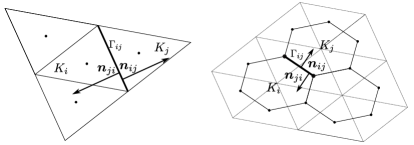
Figure 1: Finite volume patch arising from a cell-centered discretization (left) and a vertex-centered discretization (right).

4.1.2 Definitions of $({\mathcal{V}},{\mathcal{E}})$, $m_{i}$, and ${\boldsymbol{c}}_{ij}$

We define the connectivity graph $({\mathcal{V}},{\mathcal{E}})$ by identifying the vertices of this graph with the cells in ${\mathcal{T}}_{h}$, and we say that a pair of cells $K_{i},K_{j}$ form an edge of the graph, i.e., $(i,j)\in{\mathcal{E}}$, iff the cells $K_{i}$ and $K_{j}$ share an interface, i.e., $\partial K_{i}\cap\partial K_{j}$ is a $(d-1)$-manifold of positive measure. For any $i\in{\mathcal{V}}$ we define the adjacency list ${\mathcal{I}}(i)$ to be the list of all the cells in ${\mathcal{T}}_{h}$ sharing an interface with $K_{i}$, i.e., ${\mathcal{I}}(i):=\{j\in{\mathcal{V}}{\;|\;}\ (i,j)\in{\mathcal{E}}\}$, see Figure 1. Denoting by $\mathbb{I}_{K_{j}}$ the indicator function of the cell $K_{j}$, we set $X_{h}:=\operatorname{span}\{\mathbb{I}_{K_{j}}\}_{j\in{\mathcal{V}}}$ and then define the approximation space ${\boldsymbol{X}}_{h}:=(X_{h})^{m}=\{\sum_{j\in{\mathcal{V}}}\textsf{{V}}_{j}\mathbb{I}_{K_{j}}{\;|\;}\textsf{{V}}_{j}\in{\mathbb{R}}^{m},\forall j\in{\mathcal{V}}\}$.

Let ${\boldsymbol{u}}_{h}^{n}=\sum_{j\in{\mathcal{V}}}\textsf{{U}}_{j}^{n}\mathbb{I}_{K_{j}}\in{\boldsymbol{X}}_{h}$ be the approximation of ${\boldsymbol{u}}$ at time $t^{n}$, then most first-order finite volume schemes are written as follows

$$\frac{|K_{i}|}{{\tau}}(\textsf{{U}}_{i}^{\textup{L},n+1}-\textsf{{U}}_{i}^{n})+\sum_{j\in{\mathcal{I}}(i)\backslash\{i\}}\textsf{{F}}_{ij}^{\textup{L},n}=|K_{i}|{\boldsymbol{S}}(\textsf{{U}}_{i}^{n}),$$

where $\textsf{{F}}_{ij}^{\textup{L},n}$ is usually the Lax-Friedrichs/Rusanov flux (integrated over $\Gamma_{ij}$):

(4.1) $$\textsf{{F}}_{ij}^{\textup{L},n}:=\frac{|\Gamma_{ij}|}{2}({\mathbbm{f}}(\textsf{{U}}_{j}^{n})+{\mathbbm{f}}(\textsf{{U}}_{i}^{n})){\boldsymbol{n}}_{ij}-\alpha_{ij}^{\textup{L},n}(\textsf{{U}}^{n}_{j}-\textsf{{U}}^{n}_{i}),$$

where $\alpha_{ij}^{\textup{L},n}$ is some wave speed. Hence, we recover the generic expression (3.4) for the finite volume framework by setting

(4.2) $$m_{i} :=|K_{i}|,\quad{\boldsymbol{c}}_{ij}:=\frac{|\Gamma_{ij}|}{2}{\boldsymbol{n}}_{ij},\ \forall j\in{\mathcal{I}}(i)\backslash\{i\},\quad{\boldsymbol{c}}_{ii}:={\boldsymbol{0}},\quad d_{ij}^{\textup{L},n}:=\alpha_{ij}^{\textup{L},n}.$$

The definition of ${\boldsymbol{c}}_{ij}$ immediately implies that ${\boldsymbol{c}}_{ij}=-{\boldsymbol{c}}_{ij}$, and the Stokes theorem implies that $\sum_{j\in{\mathcal{I}}(i)}{\boldsymbol{c}}_{ij}=\tfrac{1}{2}\sum_{j\in{\mathcal{I}}(i)\backslash\{i\}}{\boldsymbol{n}}_{ij}|\Gamma_{ij}|=\tfrac{1}{2}\int_{\partial K_{i}}{\boldsymbol{n}}\,\,{\mathrm{d}}s={\boldsymbol{0}}$, which is the conservation property stated in (3.2). Note that $\textsf{{F}}_{ij}^{\textup{L},n}=-\textsf{{F}}_{ji}^{\textup{L},n}$ since ${\boldsymbol{n}}_{ij}=-{\boldsymbol{n}}_{ji}$. Let us mention in passing that while any family of vectors of the form ${\boldsymbol{c}}_{ij}=\alpha{\boldsymbol{n}}_{ij}|\Gamma_{ij}|$ satisfies the conservation constraint (3.2), only the factor $\alpha=\frac{1}{2}$ leads to a consistent discretization of the divergence operator.

4.2 Continuous finite elements

We describe in this section one possible implementation of the abstract low-order scheme (3.2)–(3.4) in the context of continuous finite elements (cG). The set of the $d$-variate polynomials of degree at most $k\in{\mathbb{N}}$ is denoted ${\mathbb{P}}_{k,d}$. The reader who is familiar with [19, 21, 24] is invited to move to §4.3.

4.2.1 Technical preliminaries

Let $({\mathcal{T}}_{h})_{h>0}$ be a shape-regular sequence of matching meshes. To keep some level of generality we assume that the elements in the mesh are generated from a finite number of reference elements denoted ${\widehat{K}}_{1},\dots,{\widehat{K}}_{\varpi}$. For example, the mesh ${\mathcal{T}}_{h}$ could be composed of a combination of triangles and parallelograms in dimension two (we would have $\varpi=2$ in this case); it could also be composed of a combination of tetrahedra, parallelepipeds, and triangular prisms in dimension three (we would have $\varpi=3$ in this case). The diffeomorphism mapping ${\widehat{K}}_{r}$ to an arbitrary element $K\in{\mathcal{T}}_{h}$ is denoted $T_{K}:{\widehat{K}}_{r}\longrightarrow K$. We now introduce a set of reference finite elements $\{({\widehat{K}}_{r},{\widehat{P}}_{r},{\widehat{\Sigma}}_{r})\}_{1\leq r\leq\varpi}$ (the index $r\in\{1\hskip 0.50003pt{:}\hskip 1.00006pt\varpi\}$ will be omitted in the rest of the paper to simplify the notation), and we define the following scalar-valued and vector-valued continuous finite element spaces:

(4.3) $$X_{h} =\{v\in{\mathcal{C}}^{0}(D;{\mathbb{R}}){\;|\;}v_{|K}{\circ}T_{K}\in{\widehat{P}},\ \forall K\in{\mathcal{T}}_{h}\},\qquad{\boldsymbol{X}}_{h}=[X_{h}]^{m}.$$

The global shape functions are denoted by $\{\varphi_{i}\}_{i\in{\mathcal{V}}}$ and we assume that they satisfy the partition of unity property $\sum_{i\in{\mathcal{V}}}\varphi_{i}({\boldsymbol{x}})=1$, for all ${\boldsymbol{x}}\in D$.

4.2.2 Definitions of $({\mathcal{V}},{\mathcal{E}})$, $m_{i}$, and ${\boldsymbol{c}}_{ij}$

We define the connectivity graph $({\mathcal{V}},{\mathcal{E}})$ by identifying the shape functions $\{\varphi_{i}\}_{i\in{\mathcal{V}}}$ with the vertices of the graph. The edges are defined as follows: we say that two shape functions (or two degrees of freedom) form an edge, i.e., $(i,j)\in{\mathcal{E}}$, iff $\varphi_{i}\varphi_{j}\not\equiv 0$. For any $i\in{\mathcal{V}}$, the adjacency list ${\mathcal{I}}(i)$ is defined by setting ${\mathcal{I}}(i):=\{j\in{\mathcal{V}}{\;|\;}(i,j)\in{\mathcal{E}}\}$.

Let ${\mathcal{M}}$ be the consistent mass matrix with entries $\int_{D}\varphi_{i}({\boldsymbol{x}})\varphi_{j}({\boldsymbol{x}})\,{\mathrm{d}}{\boldsymbol{x}}$, $i,j\in{\mathcal{V}}$, and let ${\mathcal{M}}^{L}$ be the diagonal lumped mass matrix with entries

(4.4) $$m_{i}:=\int_{D}\varphi_{i}({\boldsymbol{x}})\,{\mathrm{d}}{\boldsymbol{x}}.$$

The partition of unity property implies that $m_{i}=\sum_{j\in{\mathcal{I}}(i)}\int_{D}\varphi_{j}({\boldsymbol{x}})\varphi_{i}({\boldsymbol{x}})\,{\mathrm{d}}{\boldsymbol{x}}$, i.e., the entries of ${\mathcal{M}}^{L}$ are obtained by summing the rows of ${\mathcal{M}}$. In the rest of the paper we assume that $m_{i}>0$, for all $i\in{\mathcal{V}}$. This assumption is satisfied by many families of finite elements.

Let ${\boldsymbol{u}}_{h}^{n}=\sum_{j\in{\mathcal{V}}}\textsf{{U}}_{j}^{n}\varphi_{j}\in{\boldsymbol{X}}_{h}$ be the approximation of ${\boldsymbol{u}}$ at time $t^{n}$, where ${\boldsymbol{X}}_{h}$ is the continuous finite element space defined in (4.3). We approximate ${\mathbbm{f}}({\boldsymbol{u}}_{h}^{n})$ by $\sum_{j\in{\mathcal{V}}}{\mathbbm{f}}(\textsf{{U}}_{j}^{n})\varphi_{j}$. If ${\widehat{P}}$ is composed of Lagrange elements, then $\sum_{j\in{\mathcal{V}}}{\mathbbm{f}}(\textsf{{U}}_{j}^{n})\varphi_{j}$ is the Lagrange interpolation of ${\mathbbm{f}}({\boldsymbol{u}}_{h}^{n})$, and in this case the approximation is fully consistent with the polynomial degree of ${\widehat{P}}$; otherwise, the approximation is formally at least second-order accurate in space since it is exact if ${\mathbbm{f}}$ is linear. As a result, we have

(4.5) $$\int_{D}\nabla{\cdot}({\mathbbm{f}}({\boldsymbol{u}}_{h}^{n}))\varphi_{i}\,{\mathrm{d}}{\boldsymbol{x}} \approx\sum_{j\in{\mathcal{I}}(i)}{\mathbbm{f}}(\textsf{{U}}_{j}^{n})\int_{D}\varphi_{i}\nabla\varphi_{j}\,{\mathrm{d}}{\boldsymbol{x}}=\sum_{j\in{\mathcal{I}}(i)}{\mathbbm{f}}(\textsf{{U}}_{j}^{n}){\boldsymbol{c}}_{ij},$$

where the coefficients ${\boldsymbol{c}}_{ij}\in{\mathbb{R}}^{d}$ are defined by

(4.6) $${\boldsymbol{c}}_{ij}=\int_{D}\varphi_{i}\nabla\varphi_{j}\,{\mathrm{d}}{\boldsymbol{x}},\quad\forall j\in{\mathcal{I}}(i).$$

Here we observe that the partition of unity property and definition (4.6) imply that $\sum_{j\in{\mathcal{I}}(i)}{\boldsymbol{c}}_{ij}=\sum_{j\in{\mathcal{I}}(i)}\int_{D}\varphi_{i}\nabla\varphi_{j}\,{\mathrm{d}}{\boldsymbol{x}}=\int_{D}\varphi_{i}\nabla\big{(}\sum_{j\in{\mathcal{I}}(i)}\varphi_{j}\big{)}\,{\mathrm{d}}{\boldsymbol{x}}={\boldsymbol{0}}.$ On the other hand, the skew-symmetry property ${\boldsymbol{c}}_{ij}=-{\boldsymbol{c}}_{ji}$ follows using integration by parts if $D$ is the $d$-torus (which is the case for periodic boundary conditions) or if either $\varphi_{i}$ or $\varphi_{j}$ vanish at the boundary of $D$ (which is the case when we solve the Cauchy problem).

4.3 Discontinuous finite elements

We finally describe in this section one possible implementation of the abstract low-order scheme (3.2)–(3.4) in the context of discontinuous finite elements (dG). This section builds on top of the definitions and notation already introduced in §4.2.1.

4.3.1 Technical preliminaries

Here we clarify/expand on the specific details related to discontinuous spaces. We define scalar-valued and vector-valued discontinuous finite element spaces as follows:

(4.7) $$X_{h}=\{v\in L^{1}(D;{\mathbb{R}}){\;|\;}v_{|K}{\circ}T_{K}\in{\widehat{P}},\ \forall K\in{\mathcal{T}}_{h}\},\quad{\boldsymbol{X}}_{h}:=[X_{h}]^{m}.$$

We denote by $\{\varphi_{i}\}_{i\in{\mathcal{V}}}$ the collection of global shape functions generated from the reference shape functions, i.e., $X_{h}=\operatorname{span}\{\varphi_{i}\}_{i\in{\mathcal{V}}}$. Each shape function has support on one cell only. We denote by ${\mathcal{I}}(K)$ the set of indices of the shape functions with support in $K$. Similarly, letting $\partial K$ to be the boundary of the cell $K$, we denote by ${\mathcal{I}}(\partial K)$ the set of indices of the shape functions with non-vanishing trace on $\partial K$:

(4.8) $${\mathcal{I}}(K):=\big{\{}i\in{\mathcal{V}}{\;|\;}\varphi_{i|K}\not\equiv 0\big{\}},\qquad{\mathcal{I}}(\partial K):=\big{\{}i\in{\mathcal{V}}{\;|\;}\varphi_{i|\partial K}\not\equiv 0\big{\}}.$$

Note that ${\mathcal{I}}(\partial K)$ not only includes indices of shape functions with support in ${\mathcal{I}}(K)$ but this set also includes indices of shape functions that do not have support in $K$ (see Figure 2 for additional geometrical insight). More precisely ${\mathcal{I}}(\partial K)$ is the union of two disjoint sets ${\mathcal{I}}(\partial K^{\mathsf{i}})$ and ${\mathcal{I}}(\partial K^{\mathsf{e}})$ defined as

(4.9) $${\mathcal{I}}(\partial K^{\mathsf{i}}) :=\big{\{}i\in{\mathcal{I}}(K)\ \big{|}\ \varphi_{i|\partial K}\not\equiv 0\big{\}},\qquad{\mathcal{I}}(\partial K^{\mathsf{e}}):={\mathcal{I}}(\partial K)\backslash{\mathcal{I}}(\partial K^{\mathsf{i}}).$$

Finally, we assume that the finite element spaces are always constructed so that the sets of shape functions $\{\varphi_{j}\}_{j\in{\mathcal{I}}(K)}$ form a partition of unity over $K$ and the shape functions $\{\varphi_{j}\}_{j\in{\mathcal{I}}(\partial K^{\mathsf{i}})}$, $\{\varphi_{j}\}_{j\in{\mathcal{I}}(\partial K^{\mathsf{e}})}$ form partitions of unity over $\partial K$, i.e.,

(4.10) $$\sum_{j\in{\mathcal{I}}(K)}\varphi_{j|K}=1,\qquad\sum_{j\in{\mathcal{I}}(\partial K^{\mathsf{i}})}\varphi_{j|\partial K}=1,\ \text{ and }\sum_{j\in{\mathcal{I}}(\partial K^{\mathsf{e}})}\varphi_{j|\partial K}=1.$$

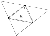
Figure 2: Discontinuous ${\mathbb{P}}_{1,2}$ finite element patch (exploded view). Each black dot represents a scalar shape function. In this picture $i\in{\mathcal{I}}(K)$, $\textup{card}({\mathcal{I}}(i))=7$, $\textup{card}({\mathcal{I}}(K))=3$, $\textup{card}({\mathcal{I}}(\partial K))=9$, $\textup{card}({\mathcal{I}}(\partial K^{\mathsf{i}}))=3$, $\textup{card}({\mathcal{I}}(\partial K^{\mathsf{e}}))=6$ and $\textup{card}({\mathcal{I}}(K)\backslash{\mathcal{I}}(\partial K^{\mathsf{i}}))=0$.

4.3.2 Definitions of $({\mathcal{V}},{\mathcal{E}})$, $m_{i}$, and ${\boldsymbol{c}}_{ij}$

We start by defining the undirected graph $({\mathcal{V}},{\mathcal{E}})$. The vertices are identified with the shape functions $\{\varphi_{i}\}_{i\in{\mathcal{V}}}$. Let $i\in{\mathcal{V}}$ and let $K$ be the unique cell containing the support of $\varphi_{i}$. For any $i,j\in{\mathcal{V}}$, we say that the pair $(i,j)$ is an edge of the connectivity graph, i.e., $(i,j)\in{\mathcal{E}}$, iff either $j\in{\mathcal{I}}(K)$ or $j\in{\mathcal{I}}(\partial K^{\mathsf{e}})$ and $\varphi_{i}\varphi_{j}|_{\partial K}\not\equiv 0$.

The consistent mass matrix and the lumped mass matrix are defined as in §4.2; in particular we set

(4.11) $$m_{i}:=\int_{D}\varphi_{i}({\boldsymbol{x}})\,{\mathrm{d}}{\boldsymbol{x}}.$$

Let ${\boldsymbol{u}}_{h}^{n}=\sum_{j\in{\mathcal{V}}}\textsf{{U}}_{j}^{n}\varphi_{j}\in{\boldsymbol{X}}_{h}$ be the approximation of ${\boldsymbol{u}}$ at time $t^{n}$, where ${\boldsymbol{X}}_{h}$ is a discontinuous finite element space defined in (4.7). Let $K\in{\mathcal{T}}_{h}$ and $i\in{\mathcal{I}}(K)$. The traditional heuristics for the derivation of dG schemes consists of integrating by parts on each cell $K$ and introducing a numerical flux $\widehat{{\mathbbm{f}}}$ on the boundary $\partial K$ as follows:

(4.12) $$\int_{K}\nabla{\cdot}({\mathbbm{f}}({\boldsymbol{u}}_{h}^{n}))\varphi_{i}\,{\mathrm{d}}{\boldsymbol{x}}\approx\int_{K}-{\mathbbm{f}}({\boldsymbol{u}}_{h}^{n}){\cdot}\nabla\varphi_{i}\,{\mathrm{d}}{\boldsymbol{x}}+\int_{\partial K}\widehat{{\mathbbm{f}}}{\boldsymbol{n}}_{K}\varphi_{i}\,{\mathrm{d}}s.$$

Upon denoting by ${\boldsymbol{u}}_{h}^{n,\mathsf{i}}$ the interior trace of ${\boldsymbol{u}}_{h}^{n}$ on $\partial K$ and ${\boldsymbol{u}}_{h}^{n,\mathsf{e}}$ the exterior trace on $\partial K$, it is common to define the numerical flux as follows:

(4.13) $$\widehat{{\mathbbm{f}}}{\boldsymbol{n}}_{K}=\frac{1}{2}({\mathbbm{f}}({\boldsymbol{u}}_{h}^{n,\mathsf{i}})+{\mathbbm{f}}({\boldsymbol{u}}_{h}^{n,\mathsf{e}})){\boldsymbol{n}}_{K}+\alpha_{\partial K}^{n}({\boldsymbol{u}}_{h}^{n,\mathsf{i}}-{\boldsymbol{u}}_{h}^{n,\mathsf{e}}),$$

where $\alpha_{\partial K}^{n}>0$ is usually some ad-hoc wave speed. The exact form of $\alpha_{\partial K}^{n}$ is unimportant for the time being; the sole purpose of the term $\alpha_{\partial K}^{n}({\boldsymbol{u}}_{h}^{i}-{\boldsymbol{u}}_{h}^{e})$ is to stabilize the algorithm. We are just going to assume that this term introduces a first-order consistency error and that we are perfectly allowed to introduce further modifications to the discrete divergence operator (4.12) consistent with this assumption. Inserting (4.13) into (4.12) and integrating by parts, we obtain

(4.14) $$\int_{K}\nabla{\cdot}({\mathbbm{f}}({\boldsymbol{u}}_{h}))\varphi_{i}\,{\mathrm{d}}{\boldsymbol{x}}\approx\int_{K}\nabla{\cdot}({\mathbbm{f}}({\boldsymbol{u}}_{h}))\varphi_{i}\,{\mathrm{d}}{\boldsymbol{x}}\\ +\int_{\partial K}\tfrac{1}{2}({\mathbbm{f}}({\boldsymbol{u}}_{h}^{\mathsf{e}})-{\mathbbm{f}}({\boldsymbol{u}}_{h}^{\mathsf{i}})){\cdot}{\boldsymbol{n}}_{K}\varphi_{i}\,{\mathrm{d}}s+\int_{\partial K}\alpha_{\partial K}^{n}({\boldsymbol{u}}_{h}^{\mathsf{i}}-{\boldsymbol{u}}_{h}^{\mathsf{e}})\varphi_{i}\,{\mathrm{d}}s.$$

We now consider an idea analogous to (4.5) and we replace ${\mathbbm{f}}({\boldsymbol{u}}_{h})$ on the right-hand side of (4.14) by $\sum_{j\in{\mathcal{V}}}{\mathbbm{f}}(\textsf{{U}}_{j}^{n})\varphi_{j}$ (where $\{\varphi_{j}\}_{j\in{\mathcal{V}}}$ are the shape functions of our discontinuous finite element space) to get:

(4.15) $$\begin{aligned} &\int_{K}\nabla{\cdot}({\mathbbm{f}}({\boldsymbol{u}}_{h}))\varphi_{i}\,{\mathrm{d}}{\boldsymbol{x}}\approx\sum_{j\in{\mathcal{I}}(K)}{\mathbbm{f}}(\textsf{{U}}_{j}^{n}){\cdot}{\boldsymbol{c}}_{ij}^{K}\\ &\ \ \ \ +\sum_{j\in{\mathcal{I}}(\partial K^{\mathsf{e}})}{\mathbbm{f}}(\textsf{{U}}_{j}^{n}){\cdot}{\boldsymbol{c}}_{ij}^{\partial}-\sum_{j\in{\mathcal{I}}(\partial K^{\mathsf{i}})}{\mathbbm{f}}(\textsf{{U}}_{j}^{n}){\cdot}{\boldsymbol{c}}_{ij}^{\partial}+\int_{\partial K}\alpha_{\partial K}^{n}({\boldsymbol{u}}_{h}^{i}-{\boldsymbol{u}}_{h}^{e})\varphi_{i}\,{\mathrm{d}}s,\end{aligned}$$

with the notation

(4.16) $${\boldsymbol{c}}_{ij}^{K}:=\int_{K}\varphi_{i}\nabla\varphi_{j}\,{\mathrm{d}}{\boldsymbol{x}},\qquad{\boldsymbol{c}}_{ij}^{\partial}:=\tfrac{1}{2}\int_{\partial K}\varphi_{j}\varphi_{i}{\boldsymbol{n}}_{K}\,{\mathrm{d}}s,$$

The three summations in (4.15) represent a consistent discretization of the divergence operator. In order to condense these three summations into a single one, and after noticing that $j$ can belong to only one of three possible (disjoint) subsets: ${\mathcal{I}}(K)\backslash{\mathcal{I}}(\partial K^{\mathsf{i}})$, ${\mathcal{I}}(\partial K^{\mathsf{i}})$ or ${\mathcal{I}}(\partial K^{\mathsf{e}})$, we define the vector ${\boldsymbol{c}}_{ij}$ by setting:

(4.17) $${\boldsymbol{c}}_{ij}:=\begin{cases}{\boldsymbol{c}}_{ij}^{K}&\text{if }j\in{\mathcal{I}}(K)\backslash{\mathcal{I}}(\partial K^{\mathsf{i}}),\\ ({\boldsymbol{c}}_{ij}^{K}-{\boldsymbol{c}}_{ij}^{\partial})&\text{if }j\in{\mathcal{I}}(\partial K^{\mathsf{i}}),\\ {\boldsymbol{c}}_{ij}^{\partial}&\text{if }j\in{\mathcal{I}}(\partial K^{\mathsf{e}}).\end{cases}$$

Therefore, (4.15) can be rewritten as follows:

(4.18) $$\begin{aligned} \int_{K}\nabla{\cdot}({\mathbbm{f}}({\boldsymbol{u}}_{h}))\varphi_{i}\,{\mathrm{d}}{\boldsymbol{x}}\approx\sum_{j\in{\mathcal{I}}(i)}{\mathbbm{f}}(\textsf{{U}}_{j}^{n}){\cdot}{\boldsymbol{c}}_{ij}+\int_{\partial K}\alpha_{\partial K}^{n}({\boldsymbol{u}}_{h}^{i}-{\boldsymbol{u}}_{h}^{e})\varphi_{i}\,{\mathrm{d}}s.\end{aligned}$$

Lemma 4.1.

The set of coefficients $\{{\boldsymbol{c}}_{ij}\}_{j\in{\mathcal{I}}(i)}$ defined in (4.17) satisfy the conservation properties (3.2). $\square$

Proof 4.2.

Let us start by proving the skew-symmetry property. Notice that (4.16) is equivalent to

$${\boldsymbol{c}}_{ij}:=\begin{cases}{\boldsymbol{c}}_{ij}^{K}-{\boldsymbol{c}}_{ij}^{\partial}&\text{if }j\in{\mathcal{I}}(K),\\ {\boldsymbol{c}}_{ij}^{\partial}&\text{if }j\in{\mathcal{I}}(\partial K^{\mathsf{e}}).\end{cases}$$

Let $j\in{\mathcal{I}}(K^{\prime})$. Assume first that $K=K^{\prime}$, then ${\boldsymbol{c}}_{ij}={\boldsymbol{c}}_{ij}^{K}-{\boldsymbol{c}}_{ij}^{\partial}$. An integration by parts gives ${\boldsymbol{c}}_{ij}=-{\boldsymbol{c}}_{ji}^{K}+{\boldsymbol{c}}_{ij}^{\partial}$, which implies that ${\boldsymbol{c}}_{ij}=-{\boldsymbol{c}}_{ji}$ because $i\in{\mathcal{I}}(K^{\prime})$. Assume now that $K\neq K^{\prime}$ but $i\in{\mathcal{I}}(\partial{K^{\prime}}^{\mathsf{e}})$, then ${\boldsymbol{c}}_{ij}={\boldsymbol{c}}_{ij}^{\partial}$. But ${\boldsymbol{n}}_{K}=-{\boldsymbol{n}}_{K^{\prime}}$, hence ${\boldsymbol{c}}_{ij}^{\partial}=-{\boldsymbol{c}}_{ji}^{\partial}$, which means that ${\boldsymbol{c}}_{ij}=-{\boldsymbol{c}}_{ji}$ because $i\in{\mathcal{I}}(\partial{K^{\prime}}^{\mathsf{e}})$.

Let us now prove that $\sum_{j\in{\mathcal{I}}(i)}{\boldsymbol{c}}_{ij}={\boldsymbol{0}}$. Using that ${\mathcal{I}}(K)\backslash{\mathcal{I}}(\partial K^{\mathsf{i}})$, ${\mathcal{I}}(\partial K^{\mathsf{i}})$, ${\mathcal{I}}(\partial K^{\mathsf{e}})$ is a partition of ${\mathcal{I}}(i)$ and definition (4.17) we have that

$$\sum_{j\in{\mathcal{I}}(i)}{\boldsymbol{c}}_{ij} =\sum_{j\in{\mathcal{I}}(K)\backslash{\mathcal{I}}(\partial K^{\mathsf{i}})}{\boldsymbol{c}}_{ij}+\sum_{j\in{\mathcal{I}}(\partial K^{\mathsf{i}})}{\boldsymbol{c}}_{ij}+\sum_{j\in{\mathcal{I}}(\partial K^{\mathsf{e}})}{\boldsymbol{c}}_{ij}$$

$$=\sum_{j\in{\mathcal{I}}(K)\backslash{\mathcal{I}}(\partial K^{\mathsf{i}})}{\boldsymbol{c}}_{ij}^{K}+\sum_{j\in{\mathcal{I}}(\partial K^{\mathsf{i}})}({\boldsymbol{c}}_{ij}^{K}-{\boldsymbol{c}}_{ij}^{\partial})+\sum_{j\in{\mathcal{I}}(\partial K^{\mathsf{e}})}{\boldsymbol{c}}_{ij}^{\partial}$$

$$=\sum_{j\in{\mathcal{I}}(K)}{\boldsymbol{c}}_{ij}^{K}-\sum_{j\in{\mathcal{I}}(\partial K^{\mathsf{i}})}{\boldsymbol{c}}_{ij}^{\partial}+\sum_{j\in{\mathcal{I}}(\partial K^{\mathsf{e}})}{\boldsymbol{c}}_{ij}^{\partial}.$$

the partition of unity property on $K$ (see (4.10)) implies that $\sum_{j\in{\mathcal{I}}(K)}{\boldsymbol{c}}_{ij}^{K}=\boldsymbol{0}$. The partition of unity property on $\partial K$ (see (4.10)) implies that $\sum_{j\in{\mathcal{I}}(\partial K^{\mathsf{i}})}{\boldsymbol{c}}_{ij}^{\partial}=\int_{\partial K}\varphi_{i}{\boldsymbol{n}}_{K}\,{\mathrm{d}}s$ and $\sum_{j\in{\mathcal{I}}(\partial K^{\mathsf{e}})}{\boldsymbol{c}}_{ij}^{\partial}=\int_{\partial K}\varphi_{i}{\boldsymbol{n}}_{K}\,{\mathrm{d}}s$; hence, the last two summations cancel each other. This completes the proof. $\square$

4.4 Graph viscosity for dG

It is important to notice at this stage, that the formulation of the viscous fluxes $\int_{\partial K}\alpha_{\partial K}^{n}({\boldsymbol{u}}_{h}^{n,\textup{i}}-{\boldsymbol{u}}_{h}^{n,\textup{e}})\varphi_{i}\,{\mathrm{d}}s$ in (4.18) is not compatible with our pursuit of a purely algebraic formulation. Note that the dissipation in (4.18) is active only on $\partial K$ and there is no dissipation in the bulk of $K$, at least when the polynomial degree of the approximation is larger than or equal to $1$. More precisely, assume for the sake of simplicity that $\alpha_{\partial K}^{n}$ is constant over $\partial K$. Let us asume also that the shape functions are Lagrange-based and let $\{{\boldsymbol{x}}_{i}\}_{i\in{\mathcal{V}}}$ be the Lagrange nodes associated with $\{\varphi_{i}\}_{i\in{\mathcal{V}}}$. Then using the quadrature generated by the Lagrange nodes, one can legitimately approximate the integral $\int_{\partial K}\alpha_{\partial K}^{n}({\boldsymbol{u}}_{h}^{n,\textup{i}}-{\boldsymbol{u}}_{h}^{n,\textup{e}})\varphi_{i}\,{\mathrm{d}}s$ by $m_{i}^{\partial}\alpha_{\partial K}^{n}({\boldsymbol{u}}_{h}^{n,\textup{i}}({\boldsymbol{x}}_{i})-{\boldsymbol{u}}_{h}^{n,\textup{e}}({\boldsymbol{x}}_{i}))$, where $m_{i}^{\partial}=\int_{\partial K}\varphi_{i}\,{\mathrm{d}}s$. This means that if $i$ and $j$ are in ${\mathcal{I}}(K)$ and $i\neq j$ (which we can assume since the polynomial degree is at least $1$), then the “stabilizing” term $\int_{\partial K}\alpha_{\partial K}^{n}({\boldsymbol{u}}_{h}^{n,\textup{i}}-{\boldsymbol{u}}_{h}^{n,\textup{e}})\varphi_{i}\,{\mathrm{d}}s$ does not contain any term proportional to ${\boldsymbol{u}}_{h}^{n,\textup{i}}({\boldsymbol{x}}_{i})-{\boldsymbol{u}}_{h}^{n,\textup{i}}({\boldsymbol{x}}_{j})$. That is to say, the traditional dG stabilization does not contain any stabilizing mechanism between the degrees of freedom that are internal to $K$. It is at this very point that we depart from the traditional dG formulation: we replace $\int_{\partial K}\alpha_{\partial K}^{n}({\boldsymbol{u}}_{h}^{i}-{\boldsymbol{u}}_{h}^{e})\varphi_{i}\,{\mathrm{d}}s$ by the graph Laplacian $-\sum_{j\in{\mathcal{I}}(i)}d_{ij}^{\textup{L},n}(\textsf{{U}}^{n}_{j}-\textsf{{U}}^{n}_{i})$ which accounts for any possible interactions inside $K$ and with the exterior traces on $\partial K$. Therefore, we finally replace (4.18) by

(4.19) $$\begin{aligned} \int_{K}\nabla{\cdot}({\mathbbm{f}}({\boldsymbol{u}}_{h}))\varphi_{i}\,{\mathrm{d}}{\boldsymbol{x}}\approx\sum_{j\in{\mathcal{I}}(i)}{\mathbbm{f}}(\textsf{{U}}_{j}^{n}){\cdot}{\boldsymbol{c}}_{ij}-\sum_{j\in{\mathcal{I}}(i)}d_{ij}^{\textup{L},n}(\textsf{{U}}^{n}_{j}-\textsf{{U}}^{n}_{i}),\end{aligned}$$

and, thus modified, the final dG scheme exactly matches the generic form of the abstract scheme (3.4).

5 Runge Kutta SSP time integration

Increasing the time accuracy while keeping the invariant domain property can be done by using so-called Strong Stability Preserving (SSP) time discretization methods. The key idea is to achieve higher-order accuracy in time by making convex combinations of forward Euler steps. More precisely each time step of a SSP method is decomposed into substeps that are all forward Euler steps; the final update is constructed as a convex combination of the intermediate solutions. This section is meant to be a brief overview of SSP methods; we refer the reader to Ferracina and Spijker [12], Higueras [27], Gottlieb et al. [16] for more detailed reviews. The main result of this section is the Shu-Osher Theorem 5.4. Our formulation of the result is slightly different from the original statement to emphasize that this result is only about convexity (i.e., it does not involve any norm, seminorm, or convex functional). The reader familiar with this material is invited to move to §6.

5.1 SSPRK methods

We are going to illustrate the SSP concept with explicit Runge Kutta methods. Let us consider a finite-dimensional vector space $E$, a subset $A\subset E$ and a (nonlinear) operator $L:[0,T]{\times}A\longrightarrow E$. We are interested in approximating in time the following problem $\partial_{t}u+L(t,u)=0$ with appropriate initial condition. We assume that this system of ordinary differential equations makes sense (for instance $L$ is continous w.r.t. $t$ and Lipschitz w.r.t. $u$). We further assume that there exists a convex subset $B\subset A$ and ${\tau}_{\max}>0$ such that

(5.1) $$v+{\tau}L(t,v)\subset B,\qquad\forall v\in B,\ \forall t\in[0,T],\ \forall{\tau}\in[0,{\tau}_{\max}].$$

Consider a general $s$ stages, explicit Runge–Kutta method identified by its Butcher tableau composed of a matrix $(a_{ij})_{\{1\leq i,j\leq s\}}\in{\mathbb{R}}^{s{\times}s}$ and a vector $(b_{j})_{\{1\leq j\leq s\}}\in{\mathbb{R}}^{s}$

(5.2) $$\begin{array}[]{c|ccccc}0\\ c_{2}&a_{21}\\ c_{3}&a_{31}&a_{32}\\ \vdots&\vdots&&\ddots&\\ c_{s}&a_{s1}&a_{s2}&\cdots&a_{s,s-1}\\ \hline\cr&b_{1}&b_{2}&\cdots&b_{s-1}&b_{s}\end{array}$$

where $c_{i}:=\sum_{j=1}^{i-1}a_{ij}$ for $i\in\{2\hskip 0.50003pt{:}\hskip 1.00006pts\}$. Let us also set $c_{1}:=0$. Let us assume now that the above $s$ stages, explicit Runge Kutta method has the following $(\alpha-\beta)$ representation: There are real coefficients $\alpha_{ki}$, $\beta_{ki}$ with $k\in\{0\hskip 0.50003pt{:}\hskip 1.00006pti-1\}$ and $i\in\{1\hskip 0.50003pt{:}\hskip 1.00006pts\}$ such that $u^{n+1}$ is obtained by first setting $w^{(0)}=u^{n}$, then computing

(5.3) $$w^{(i)} =\sum_{k=0}^{i-1}\alpha_{ik}w^{(k)}+\beta_{ik}{\tau}L(t^{n}+\gamma_{k}{\tau},w^{(k)}),\quad i\in\{1\hskip 0.50003pt{:}\hskip 1.00006pts\},$$

and finally setting $u^{n+1}=w^{(s)}$, where $\sum_{0\leq k\leq i-1}\alpha_{ik}=1$, $\gamma_{k}:=c_{k+1}$, $\alpha_{ik}\geq 0$, and $\beta_{ik}\geq 0$, for all $k\in\{0\hskip 0.50003pt{:}\hskip 1.00006pti-1\}$ and all $i\in\{1\hskip 0.50003pt{:}\hskip 1.00006pts\}$. We further assume that $\beta_{ik}=0$ if $\alpha_{ik}=0$, $k\in\{0\hskip 0.50003pt{:}\hskip 1.00006pti-1\}$, $i\in\{1\hskip 0.50003pt{:}\hskip 1.00006pts\}$. Not every $s$ stages, explicit Runge Kutta method admits an $(\alpha-\beta)$ representation. Any Runge Kutta method that admits an $(\alpha-\beta)$ representation as defined above is said to be SSP for a reason that will be stated in Theorem 5.4.

Example 5.1 (Midpoint rule).

The midpoint rule, defined by the Butcher tableau

(5.4) $$\begin{array}[]{c|ccccc}0\\ \frac{1}{2}&\frac{1}{2}\\[2.0pt] \hline\cr&0&1\end{array}$$

does not have a legitimate $(\alpha-\beta)$ representation, since it would require that $\beta_{20}+\alpha_{21}=0$, which in turn would imply that either $\beta_{20}<0$ or $\alpha_{21}<0$. $\square$

Example 5.2 (SSPRK(2,2)).

Heun’s method, which is a second-order Runge–Kutta technique composed of two stages, is SSP. It has the following $(\alpha-\beta)$ tableau and can be implemented as follows:

$$\begin{array}[]{|cc|cc|c|c|}\hline\cr\alpha&&\beta&&\gamma&c_{\textup{os}}\\ \hline\cr\hline\cr\rule[0.0pt]{0.0pt}{10.00002pt}1&&1&&0&\\ \rule[0.0pt]{0.0pt}{10.00002pt}\frac{1}{2}&\frac{1}{2}&0&\frac{1}{2}&1&1\\[2.0pt] \hline\cr\end{array}\qquad\qquad\begin{aligned} w^{(1)}&=u^{n}\!+{\tau}L(t^{n},u^{n}),\\ w^{(2)}&=w^{(1)}\!+{\tau}L(t^{n+1},w^{(1)}),\\ u^{n+1}&=\tfrac{1}{2}u^{n}\!+\tfrac{1}{2}w^{(2)}.\end{aligned}$$

$\square$

Example 5.3 (SSPRK(3,3), SSPRK(4,3)).

The following Runge–Kutta methods, which are third-order and composed of three substeps and four substeps, respectively, are SSP:

$$\begin{array}[]{|ccc|ccc|c|c|}\hline\cr&\alpha&&&\beta&&\gamma&c_{\textup{os}}\\ \hline\cr\hline\cr\rule[0.0pt]{0.0pt}{10.00002pt}1&&&1&&&0&\\ \rule[0.0pt]{0.0pt}{10.00002pt}\frac{3}{4}&\frac{1}{4}&&0&\frac{1}{4}&&1&1\\ \rule[0.0pt]{0.0pt}{10.00002pt}\frac{1}{3}&0&\frac{2}{3}&0&0&\frac{2}{3}&\frac{1}{2}&\\[2.0pt] \hline\cr\end{array}\qquad\qquad\begin{array}[]{|cccc|cccc|c|c|}\hline\cr&\alpha&&&&\beta&&&\gamma&c_{\textup{os}}\\ \hline\cr\hline\cr\rule[0.0pt]{0.0pt}{10.00002pt}1&&&&\frac{1}{2}&&&&0&\\ \rule[0.0pt]{0.0pt}{10.00002pt}0&1&&&0&\frac{1}{2}&&&\frac{1}{2}&2\\ \rule[0.0pt]{0.0pt}{10.00002pt}\frac{2}{3}&0&\frac{1}{3}&&0&0&\frac{1}{6}&&1&\\ \rule[0.0pt]{0.0pt}{10.00002pt}0&0&0&1&0&0&0&\frac{1}{2}&\frac{1}{2}&\\[2.0pt] \hline\cr\end{array}$$

For instance the SSPRK$(3,3)$ method can be implemented as follows:

$$w^{(1)} =u^{n}+{\tau}L(t^{n},u^{n}), z^{(1)}=w^{(1)}+{\tau}L(t^{n}+{\tau},w^{(1)}),$$

$$w^{(2)} =\frac{3}{4}u^{n}+\frac{1}{4}z^{(1)},\quad z^{(2)}=w^{(2)}+{\tau}L(t^{n}+\tfrac{1}{2}{\tau},w^{(2)}),$$

$$u^{n+1} =\frac{1}{3}u^{n}+\frac{2}{3}z^{(2)}.$$

$\square$

5.2 The key result

We henceforth denote

(5.5) $$c_{\textup{os}}:=\inf_{\{\alpha_{ik}\not=0,\ 1\leq k+1\leq i\leq s\}}\alpha_{ik}\beta_{ik}^{-1}.$$

The following theorem is the main result of this section.

Theorem 5.4 (Shu-Osher).

Assume that the Runge Kutta method with the Butcher tableau (5.2) is SSP. Let $B\subset A$ be convex. Let $u^{n}\in B$ and assume that ${\tau}\leq c_{\textup{os}}{\tau}_{\max}$, then $u^{n+1}\in B$. $\square$

Proof 5.5.

Let $n\geq 0$ and assume that $u^{n}\in B$. Let $i\in\{1\hskip 0.50003pt{:}\hskip 1.00006pts\}$ and assume that $w^{(k)}\in B$ for all $k\in\{0\hskip 0.50003pt{:}\hskip 1.00006pti-1\}$. Note that this assumption is satisfied for $i=1$ since $w^{(0)}=u^{n}\in B$. Consider the $k$th term in (5.3), $0\leq k\leq i-1$. If $\alpha_{ik}=0$ then $\beta_{ik}=0$ by construction, and there is nothing to sum. Assume now that $\alpha_{ik}>0$. Let us denote $r_{ik}:=\beta_{ik}/\alpha_{ik}$ and $z^{(i,k)}:=w^{(k)}+r_{ik}{\tau}L(t^{n}+\gamma_{k}{\tau},w^{(k)})$, then the condition ${\tau}\leq c_{\textup{os}}{\tau}_{\max}$ implies that $r_{ik}{\tau}\leq(\beta_{ik}/\alpha_{ik})c_{\textup{os}}{\tau}_{\max}\leq{\tau}_{\max}$, which, owing to (5.1), is sufficient to ascertain that $z^{(i,k)}\in B$ for all $k\in\{0\hskip 0.50003pt{:}\hskip 1.00006pti-1\}$. Observing that $w^{(i)}=\sum_{k=1}^{i-1}\alpha_{ki}z^{(i,k)}$, the condition $\sum_{0\leq k\leq i-1}\alpha_{ik}=1$ together with $0\leq\alpha_{ik}$, $0\leq k\leq i-1$, implies that $w^{(i)}$ is a convex combination of $z^{(i,0)},\ldots,z^{(i,i-1)}$; hence $w^{(i)}$ is in $B$ since $B$ is convex. In conclusion $w^{(k)}\in B$ for all $k\in\{0\hskip 0.50003pt{:}\hskip 1.00006pti\}$ and all $i\in\{1\hskip 0.50003pt{:}\hskip 1.00006pts\}$, thereby proving that $u^{n+1}=w^{(s)}\in B$. $\square$

Remark 5.6 (Literature).

Theorem 5.4 has been established in a slightly different form in Shu and Osher [44, Prop. 2.1] not explicitly invoking convexity. Although our proof is very similar to that in [44], the statement of Theorem 5.4 is slightly different since it only involves convexity; no norm or seminorm (as in Gottlieb et al. [15, p. 92]), or convex functional (as in [16, Eq. (1.3)]) is involved. This variant of the theorem does not seem to be very well known. $\square$

Remark 5.7 (Structure of $B$).

In the original paper [44] and in [15], $E$ is a normed vector space equipped with some norm $\|\cdot\|_{E}$. The assumption (5.1) then consists of stating that ${\mathbb{I}}+{\tau}L(t,\cdot)$ maps any ball $B$ centered at $0$ into $B$ for any $s\in[0,{\tau}_{\max}]$ and any $t\in[0,T]$. In particular taking any $v\in E$ and defining $B$ to be the ball of radius $\|v\|_{B}$ centered at $0$, the assumption (5.1) amounts to saying that $\|v+{\tau}L(t,v)\|_{B}\leq\|v\|_{B}$, which is Eq. (1.3) in [15]. The norm that is used in [44] is the total variation. In the present paper the assumption (5.1) is more general. We are going to use it with the following structure: we are going to assume that there are two positive integers $I,m\in{\mathbb{N}}{\setminus}\{0\}$ such that $E=({\mathbb{R}}^{m})^{I}$. Here ${\mathbb{R}}^{m}$ is called the phase space. Then we assume that there is convex subset of the phase space ${\mathcal{B}}\subset{\mathbb{R}}^{m}$ such that the assumption (5.1) holds with $B:=({\mathcal{B}})^{I}$. All the convex arguments invoked in the rest of the paper extends to SSP RK techniques with this particular structure. $\square$

6 High-order method

The algorithm that we are going to develop in §7 relies on the construction of the low-order invariant domain preserving solution $\textsf{{U}}_{i}^{\textup{L},n+1}$ described in §3.1-§3.2 and a high-order solution $\textsf{{U}}_{i}^{\textup{H},n+1}$ that possibly wanders outside the invariant domain. We are then going to limit the high-order solution by pushing it back into the invariant domain in the direction of the low-order solution. This limiting technique, which we call convex limiting, will be explained in §7. The purpose of the present section is to present various ways to construct $\textsf{{U}}_{i}^{\textup{H},n+1}$.

6.1 Achieving high-order consistency

In this section we describe in broad terms how high-order consistency can be achieved.

6.1.1 Discretization-independent setting

Independently of the space discretization that is used, we henceforth assume that the high-order update $\textsf{{U}}_{i}^{\textup{H},n+1}$ is computed as follows:

(6.1) $$\frac{m_{i}}{{\tau}}(\textsf{{U}}_{i}^{\textup{H},n+1}-\textsf{{U}}_{i}^{n})+\sum_{j\in{\mathcal{I}}(i)}\textsf{{F}}_{ij}^{\textup{H},n}=m_{i}{\boldsymbol{S}}(\textsf{{U}}_{i}^{n}),$$

where the high-order flux $\textsf{{F}}_{ij}^{\textup{H},n}$ is assumed to be skew-symmetric; i.e., $\textsf{{F}}_{ij}^{\textup{H},n}=-\textsf{{F}}_{ji}^{\textup{H},n}$ for all $i\in{\mathcal{V}}$, $j\in{\mathcal{I}}(i)$ (under appropriate boundary conditions). The skew-symmetry implies that the high-order update is conservative; i.e., $\sum_{i\in{\mathcal{V}}}m_{i}\textsf{{U}}_{i}^{\textup{H},n+1}=\sum_{i\in{\mathcal{V}}}m_{i}\textsf{{U}}_{i}^{n}$ if ${\boldsymbol{S}}\equiv{\boldsymbol{0}}$. The expression (6.1) is the only information regarding the high-order update that will be necessary for the convex limiting technique to be presented in section §7.

There are many different techniques to compute high-order consistent fluxes $\textsf{{F}}_{ij}^{\textup{H},n}$ which depend on the space discretization of choice. For the sake of completeness, we list some of those in §6.1.2, §6.1.3, and §6.1.4. None of this material is essential to understand the convex limiting technique explained in §7.

6.1.2 High-order algebraic fluxes: Finite Volumes

In the context of finite volume schemes, high-order algebraic fluxes $\textsf{{F}}_{ij}^{\textup{H},n}$ are obtained as integrals of high-order numerical fluxes over the interfaces between volumes, i.e., $\textsf{{F}}_{ij}^{\textup{H},n}:=\int_{\Gamma_{ij}}\widehat{{\mathbbm{f}}}{\boldsymbol{n}}_{ij}\,{\mathrm{d}}s$ where $\widehat{{\mathbbm{f}}}{\boldsymbol{n}}_{ij}$ is some numerical flux. For instance, a widely popular choice of algebraic flux consists of setting:

(6.2) $$\textsf{{F}}_{ij}^{\textup{H},n}:=\int_{\Gamma_{ij}}\left(\tfrac{1}{2}({\mathbbm{f}}({\boldsymbol{u}}_{h}^{\mathrm{H},n,\mathsf{i}})+{\mathbbm{f}}({\boldsymbol{u}}_{h}^{\mathrm{H},n,\mathsf{e}})){\cdot}{\boldsymbol{n}}_{ij}+d_{ij}^{\textup{L},n}({\boldsymbol{u}}_{h}^{\mathrm{H},n,\mathsf{i}}-{\boldsymbol{u}}_{h}^{\mathrm{H},n,\mathsf{e}})\right)\,{\mathrm{d}}s,$$

where the superscripts $\mathsf{e}$ and $\mathsf{i}$ denote the exterior and interior traces respectively, and ${\boldsymbol{u}}_{h}^{\textup{H},n}$ is a discontinuous piecewise polynomial reconstruction (of degree at most $k$) recovered from the piecewise constant solution ${\boldsymbol{u}}_{h}^{n}=\sum_{j\in{\mathcal{V}}}\textsf{{U}}_{j}^{n}\mathbb{I}_{K_{j}}$ satisfying the conservation constraint $\frac{1}{|K_{i}|}\int_{K_{i}}({\boldsymbol{u}}_{h}^{\textup{H},n}-{\boldsymbol{u}}_{h}^{n})\,{\mathrm{d}}{\boldsymbol{x}}=0$. More precisely ${\boldsymbol{u}}_{h}^{\mathrm{H},n,\mathsf{i}}({\boldsymbol{x}})=\lim_{K_{i}\ni{\boldsymbol{y}}\to{\boldsymbol{x}}}{\boldsymbol{u}}_{h}^{\textup{H},n}({\boldsymbol{y}})$ and ${\boldsymbol{u}}_{h}^{\mathrm{H},n,\mathsf{e}}({\boldsymbol{x}})=\lim_{K_{j}\ni{\boldsymbol{y}}\to{\boldsymbol{x}}}{\boldsymbol{u}}_{h}^{\textup{H},n}({\boldsymbol{y}})$. In practice, (6.2) has to be computed using quadrature on the faces of the element. The choices of numerical flux $\widehat{{\mathbbm{f}}}{\boldsymbol{n}}_{ij}$ and reconstruction ${\boldsymbol{u}}_{h}^{\textup{H},n}$ that could be used in (6.2) are not unique. There is a massive body of literature on this topic and it is well beyond the scope of the current paper to elaborate further in this direction; we refer the reader to Barth and Ohlberger [4], Kröner [35], Morton and Sonar [39] for additional background. For the purpose of the present paper, we are only going to assume that (6.1) holds with skew-symmetric algebraic fluxes $\textsf{{F}}_{ij}^{\textup{H},n}$.

6.1.3 High-order algebraic flux: Continuous Finite Elements

We now turn our attention to continuous finite elements. In this case high-order consistency can be achieved by using a degenerate graph viscosity $d_{ij}^{\textup{H},n}$ such that $d_{ij}^{\textup{H},n}\ll d_{ij}^{\textup{L},n}$ in smooth regions while $d_{ij}^{\textup{H},n}\approx d_{ij}^{\textup{L},n}$ near shocks. Of course $d_{ij}^{\textup{H},n}$ must also satisfy the conservation constraints

(6.3) $$d_{ij}^{\textup{H},n}=d_{ji}^{\textup{H},n}\geq 0\quad\text{if $i\not=j$,}\quad\text{and}\quad\sum_{j\in{\mathcal{I}}(i)}d_{ij}^{\textup{H},n}=0.$$

The algebraic flux looks as the one defined in (3.6) for the low-order method; the only difference here is that we use the high-order viscosities $\{d_{ij}^{\textup{H},n}\}_{j\in{\mathcal{I}}(i)}$:

(6.4) $$\textsf{{F}}_{ij}^{\textup{H},n}:=({\mathbbm{f}}(\textsf{{U}}_{j}^{n})+{\mathbbm{f}}(\textsf{{U}}_{i}^{n})){\boldsymbol{c}}_{ij}-d_{ij}^{\textup{H},n}(\textsf{{U}}^{n}_{j}-\textsf{{U}}^{n}_{i}).$$

Higher-order accuracy in space can also be obtained by using the consistent mass matrix instead of the lumped mass matrix for the discretization of the time derivative. By reducing dispersive errors, this technique is known to yield superconvergence at the grid points; see Christon et al. [9], Guermond and Pasquetti [18]. In this case the high-order update is computed by solving the following mass matrix problem:

(6.5) $$\sum_{j\in{\mathcal{I}}(i)}\!\!\frac{m_{ij}}{{\tau}}(\textsf{{U}}_{j}^{\textup{H},n+1}\!-\textsf{{U}}_{j}^{n})+({\mathbbm{f}}(\textsf{{U}}_{j}^{n})+{\mathbbm{f}}(\textsf{{U}}_{i}^{n})){\boldsymbol{c}}_{ij}-d_{ij}^{\textup{H},n}(\textsf{{U}}^{n}_{j}-\textsf{{U}}^{n}_{i})=m_{i}{\boldsymbol{S}}(\textsf{{U}}_{i}^{n}).$$

Noticing that $m_{ij}=\delta_{ij}m_{i}+m_{ij}-\delta_{ij}m_{i}$, we can rewrite (6.5) as

(6.6) $$\begin{aligned} \frac{m_{i}}{{\tau}}(\textsf{{U}}_{i}^{\textup{H},n+1}-\textsf{{U}}_{i}^{n})&+\sum_{j\in{\mathcal{I}}(i)}\frac{(m_{ij}-\delta_{ij}m_{i})}{{\tau}}(\textsf{{U}}_{j}^{\textup{H},n+1}-\textsf{{U}}_{j}^{n})\\ &+({\mathbbm{f}}(\textsf{{U}}_{j}^{n})+{\mathbbm{f}}(\textsf{{U}}_{i}^{n})){\boldsymbol{c}}_{ij}-d_{ij}^{\textup{H},n}(\textsf{{U}}^{n}_{j}-\textsf{{U}}^{n}_{i})=m_{i}{\boldsymbol{S}}(\textsf{{U}}_{i}^{n}).\end{aligned}$$

Since $\sum_{j\in{\mathcal{I}}(i)}(m_{ij}-\delta_{ij}m_{i})=0$, we add $-\sum_{j\in{\mathcal{I}}(i)}\frac{(m_{ij}-\delta_{ij}m_{i})}{{\tau}}(\textsf{{U}}_{i}^{\textup{H},n+1}-\textsf{{U}}_{i}^{n})=0$ to the identity (6.6) to get

(6.7) $$\begin{aligned} \frac{m_{i}}{{\tau}}(\textsf{{U}}_{i}^{\textup{H},n+1}-\textsf{{U}}_{i}^{n})&+\sum_{j\in{\mathcal{I}}(i)\backslash\{i\}}\frac{(m_{ij}-\delta_{ij}m_{i})}{{\tau}}(\textsf{{U}}_{j}^{\textup{H},n+1}-\textsf{{U}}_{j}^{n}-\textsf{{U}}_{i}^{\textup{H},n+1}+\textsf{{U}}_{i}^{n})\\ &+({\mathbbm{f}}(\textsf{{U}}_{j}^{n})+{\mathbbm{f}}(\textsf{{U}}_{i}^{n})){\boldsymbol{c}}_{ij}-d_{ij}^{\textup{H},n}(\textsf{{U}}^{n}_{j}-\textsf{{U}}^{n}_{i})=m_{i}{\boldsymbol{S}}(\textsf{{U}}_{i}^{n}).\end{aligned}$$

Then (6.1) holds with the following definition for the high-order algebraic flux:

(6.8) $$\textsf{{F}}_{ij}^{\textup{H},n}:= {}\frac{m_{ij}}{{\tau}}(\textsf{{U}}_{j}^{\textup{H},n+1}-\textsf{{U}}_{j}^{n}-\textsf{{U}}_{i}^{\textup{H},n+1}+\textsf{{U}}_{i}^{n})$$

$$+({\mathbbm{f}}(\textsf{{U}}_{j}^{n})+{\mathbbm{f}}(\textsf{{U}}_{i}^{n})){\boldsymbol{c}}_{ij}-d_{ij}^{\textup{H},n}(\textsf{{U}}^{n}_{j}-\textsf{{U}}^{n}_{i}).$$

In the context of finite difference methods, a scheme with the above structure is said to be linearly implicit as the numerical fluxes depend linearly on the state $\textsf{{U}}_{j}^{\textup{H},n+1}$.

We finally mention a third approach which has antidispersive properties that are similar to (6.5) but does not require solving a mass matrix problem a each time step. This method consists of approximating the inverse of ${\mathcal{M}}$ by $({\mathcal{M}}^{L})^{-1}({\mathcal{I}}+({\mathcal{M}}^{L}-{\mathcal{M}})({\mathcal{M}}^{L})^{-1})$, where ${\mathcal{I}}$ is the identity matrix. We refer the reader to Guermond et al. [22, §3.3] for the details.

6.1.4 High-order algebraic flux: Discontinuous Finite Elements

Just like for continuous finite elements, high-order consistency is space is obtained for discontinuous finite elements by replacing the low-order graph viscosity $d_{ij}^{\textup{L},n}$ by a high-order graph viscosity $d_{ij}^{\textup{H},n}$ satisfying the symmetry and positivity properties stated in (6.3). The corresponding flux in (6.1) is

(6.9) $$\textsf{{F}}_{ij}^{\textup{H},n}:=({\mathbbm{f}}(\textsf{{U}}_{j}^{n})+{\mathbbm{f}}(\textsf{{U}}_{i}^{n})){\boldsymbol{c}}_{ij}-d_{ij}^{\textup{H},n}(\textsf{{U}}^{n}_{j}-\textsf{{U}}^{n}_{i}),\qquad\forall{\mathcal{I}}(K)\cup{\mathcal{I}}(K^{\mathsf{e}}).$$

Like for continuous elements, superconvergence can be obtained by using the consistent mass matrix. A high-order discontinuous finite element scheme using the consistent mass matrix can be written as follows:

(6.10) $$\sum_{j\in{\mathcal{I}}(K)}\frac{m_{ij}}{{\tau}}(\textsf{{U}}_{j}^{\textup{H},n+1}-\textsf{{U}}_{j}^{n})+\sum_{j\in{\mathcal{I}}(i)}({\mathbbm{f}}(\textsf{{U}}_{j}^{n})+{\mathbbm{f}}(\textsf{{U}}_{j}^{n})){\boldsymbol{c}}_{ij}\\ -d_{ij}^{\textup{H},n}(\textsf{{U}}^{n}_{j}-\textsf{{U}}^{n}_{i})=m_{i}{\boldsymbol{S}}(\textsf{{U}}_{i}^{n}).$$

Notice that the mass matrix only involves the dofs in ${\mathcal{I}}(K)$. As in the continuous case, noting that $m_{ij}=\delta_{ij}m_{i}+m_{ij}-\delta_{ij}m_{i}$, using the partition of unity properties, and proceeding as in (6.6)-(6.7)), we obtain the following definition for the high-order flux $\textsf{{F}}_{ij}^{\textup{H},n}$ that is used in (6.1):

(6.11) $$\textsf{{F}}_{ij}^{\textup{H},n}:=\begin{cases}\dfrac{m_{ij}}{{\tau}}(\textsf{{U}}_{j}^{\textup{H},n+1}-\textsf{{U}}_{j}^{n}-\textsf{{U}}_{i}^{\textup{H},n+1}+\textsf{{U}}_{i}^{n})&\\[2.0pt] \qquad+({\mathbbm{f}}(\textsf{{U}}_{j}^{n})+{\mathbbm{f}}(\textsf{{U}}_{i}^{n})){\boldsymbol{c}}_{ij}-d_{ij}^{\textup{H},n}(\textsf{{U}}^{n}_{j}-\textsf{{U}}^{n}_{i})&\ \ \text{if }j\in{\mathcal{I}}(K),\\[4.0pt] ({\mathbbm{f}}(\textsf{{U}}_{j}^{n})+{\mathbbm{f}}(\textsf{{U}}_{i}^{n})){\boldsymbol{c}}_{ij}-d_{ij}^{\textup{H},n}(\textsf{{U}}^{n}_{j}-\textsf{{U}}^{n}_{i})&\ \ \text{if }j\in{\mathcal{I}}(K^{\mathsf{e}}).\end{cases}$$

6.2 Smoothness-based graph viscosity

The objective of this section is to present a method where the high-order graph viscosity in (6.4), (6.8), (6.9), or (6.11) is obtained by estimating the smoothness of some functional (e.g., an entropy) of the current solution.

6.2.1 Principles of the method

Let ${\boldsymbol{u}}_{h}^{n}=\sum_{i\in{\mathcal{V}}}\textsf{{U}}_{i}^{n}\varphi_{i}$ be the current approximation and let $g:{\mathcal{A}}\to{\mathbb{R}}$ be some functional (examples will be given below). We define the smoothness indicator associated to $g$ as follows:

(6.12) $$\alpha_{i}^{n}:=\frac{\left|\sum_{j\in{\mathcal{I}}(i)}\beta_{ij}(g(\textsf{{U}}_{j}^{n})-g(\textsf{{U}}_{i}^{n}))\right|}{\max(\sum_{j\in{\mathcal{I}}(i)}|\beta_{ij}||g(\textsf{{U}}_{j}^{n})-g(\textsf{{U}}_{i}^{n})|,\epsilon_{i})},$$

with $\epsilon_{i}=\epsilon\max_{j\in{\mathcal{I}}(i)}|g(\textsf{{U}}_{j}^{n})|$, where $\epsilon$ is very small number. This term avoids degeneracy when $g(\textsf{{U}}_{j}^{n})$ is constant for all $j\in{\mathcal{I}}(i)$; see Remark 6.1. The real numbers $\beta_{ij}$ are selected to make the method linearity-preserving (see Berger et al. [5] for a review on linearity-preserving limiters in the finite volume literature). The reader is referred to Remark 6.2 for the details. Notice that $\alpha_{i}^{n}\in[0,1]$ for all $i\in{\mathcal{V}}$ and $\alpha_{i}^{n}=1$ if $g(\textsf{{U}}_{i})$ is a local extremum. This property will play an important role in the proof of Theorem 6.6 which is the main result of §6.2.

We now define the high-order graph viscosity by setting

(6.13) $$d_{ij}^{\textup{H},n}:=d_{ij}^{\textup{L},n}\max(\psi(\alpha_{i}^{n}),\psi(\alpha_{j}^{n})),$$

where $\psi\in\text{Lip}([0,1];[01,])$ is any Lipschitz function from $[0,1]$ to $[0,1]$ such that $\psi(1)=1$. One typical example is $\psi(\alpha)=\big{(}\frac{\alpha-\alpha_{0}}{1-\alpha_{0}}\big{)}^{q}$ with $q\geq 2$ and $\alpha_{0}\in[0,1)$. For instance one can take $\alpha_{0}=\frac{1}{2}$ and $q=4$. One need to be careful though not to take $\alpha_{0}$ too close to $1$ and $q$ not too large since we will see in Theorem 6.6 below that the Lipschitz constant of $\psi$ plays a important role in the properties of the method.

Remark 6.1 (Choices for $\epsilon$).

Using double precision arithmetic, the regularization in (6.12) can be done with $\epsilon=10^{-\frac{16}{2}}$. We have also observed that using $\epsilon=(m_{i}/|D|)^{\frac{3}{d}}$ maintains the second-order accuracy properties of the method in any $L^{q}$-norm, $q\in[1,\infty]$. $\square$

Remark 6.2 (Linearity-preserving $\beta_{ij}$).

To be linearity-preserving with continuous finite elements one should obtain $\alpha_{i}^{n}=0$ if $g({\boldsymbol{u}}_{h}^{n})$ is linear on the support of the shape function $\varphi_{i}$. One simple choice for continuous finite elements consists of setting $\beta_{ij}=\int_{D}\nabla\varphi_{i}{\cdot}\nabla\varphi_{j}\,{\mathrm{d}}x$ (for the time being we do not require $\beta_{ij}>0$ in (6.12)). For discontinuous elements, one could take $\beta_{ij}=\int_{K}\nabla\varphi_{j}{\cdot}\nabla\varphi_{i}\,{\mathrm{d}}x-\int_{\partial K}\frac{1}{2}\nabla\varphi_{j}{\cdot}{\boldsymbol{n}}_{K}\varphi_{i}\,{\mathrm{d}}x$, where $K$ is the unique cell such that $i\in{\mathcal{I}}(K)$ and ${\boldsymbol{n}}_{K}$ is the unit normal vector on $\partial K$ pointing outward $K$. For finite volumes, one should get $\alpha_{i}^{n}=0$ if a linear reconstruction fits all the data $\{g(\textsf{{U}}_{j}^{n})\}_{j\in{\mathcal{I}}(i)}$. For instance, one can use the mean-value coordinates; see Floater [13, Eq. 5.1] for the details. Let us finally remark that although using $\beta_{ij}=1$ is not a priori linearity preserving, we have numerically verified that this choice works reasonably well on quasi-uniform meshes. $\square$

If the coefficients $\beta_{ij}$ are defined so the linearity-preserving property holds, then the numerator of (6.12) behaves like $h^{2}\|D^{2}g({\boldsymbol{u}}({\boldsymbol{\xi}},t^{n}))\|_{\ell^{2}({\mathbb{R}}^{d{\times}d})}$ at some point ${\boldsymbol{\xi}}$, whereas the denominator behaves like $h\|\nabla g({\boldsymbol{\zeta}})\|_{\ell^{2}({\mathbb{R}}^{d})}$ at some point ${\boldsymbol{\zeta}}$. Therefore, we have $\alpha_{i}^{n}\approx h\|D^{2}g({\boldsymbol{\xi}})\|_{\ell^{2}({\mathbb{R}}^{d{\times}d})}/\|\nabla g({\boldsymbol{\zeta}})\|_{\ell^{2}({\mathbb{R}}^{d})}$, that is to say $\alpha_{i}^{n}$ is of order $h$ in the regions where $g$ is smooth and does not have a local extremum. This argument shows that $d_{ij}^{\textup{H},n}$ is one order smaller than $d_{ij}^{\textup{L},n}$ (in terms of mesh size). Hence it is reasonable to expect that the method using $d_{ij}^{\textup{H},n}$ is formally second-order accurate in space.

Example 6.3 (Choosing $g(\textsf{{U}})$).

In the context of the shallow water equations one can use the water height as smoothness indicator. For the compressible Euler equations one can use the density. We are going to prove stability properties for these two choices in Theorem 6.6, (see also Example 6.8). In general it is a good idea to choose $g(\textsf{{U}})$ to be entropy associated with (1.1) (with or without the source term). We refer the reader to Guermond et al. [24], where a full set of tests is reported for the compressible Euler equations with the $\gamma$-law. The computations therein are done with $g(\textsf{{U}})=\frac{\rho}{\gamma-1}\log(e(\textsf{{U}})\rho^{1-\gamma})$, where $e(\textsf{{U}})$ is the specific internal energy $\square$

6.2.2 Stability

We now establish some invariant domain preserving properties associated with the smoothness-based graph viscosity (6.12) when the coefficients $\beta_{ij}$ are positive. We further specialize the setting by assuming that $g:{\mathcal{A}}\to{\mathbb{R}}$ is a projection onto one of the scalar components of U. Without loss of generality we set $g(\textsf{{U}})={\mathsf{U}}_{1}$ with the convention $\textsf{{U}}:=({\mathsf{U}}_{1},\ldots,{\mathsf{U}}_{m})^{\mathsf{T}}$. From now on, we drop the index ₁ to simplify the notation; that is, we set $g(\textsf{{U}})={\mathsf{U}}$. We denote by $S:{\mathcal{A}}\to{\mathbb{R}}$ the corresponding scalar component of the source ${\boldsymbol{S}}$. One important assumption in this section is that $S\equiv 0$, i.e., the scalar component of the source acting on ${\mathsf{U}}$ is zero.

We have seen in Theorem 3.8 that the auxiliary states $\overline{\textsf{{U}}}_{ij}^{n}$ defined in (3.8) play an important role in the stability analysis. These states are such that if $\textsf{{U}}_{i}^{n},\textsf{{U}}_{j}^{n}\in{\mathcal{B}}$, where ${\mathcal{B}}\subset{\mathcal{A}}$ is some convex invariant set, then $\overline{\textsf{{U}}}_{ij}^{n}\in{\mathcal{B}}$, provided that $1+\frac{2{\tau}d_{ii}^{\textup{L},n}}{m_{i}}\geq 0$, and the low-order graph viscosity $d_{ij}^{\textup{L},n}$ is defined as in (3.10). We denote by $\overline{{\mathsf{U}}}_{ij}^{n}$ the scalar component of $\overline{\textsf{{U}}}_{ij}^{n}$ that is of interest to us. Then we set

(6.14) $${\mathsf{U}}_{i}^{\textup{M},n}:=\max_{j\in{\mathcal{I}}(i)}\overline{{\mathsf{U}}}_{ij}^{n},\qquad{\mathsf{U}}_{i}^{\textup{m},n}:=\min_{j\in{\mathcal{I}}(i)}\overline{{\mathsf{U}}}_{ij}^{n}.$$

We set ${\mathcal{I}}(i^{+}):=\{j\in{\mathcal{I}}(i){\;|\;}{\mathsf{U}}_{i}^{n}<{\mathsf{U}}_{j}^{n}\}$ and ${\mathcal{I}}(i^{-}):=\{j\in{\mathcal{I}}(i){\;|\;}{\mathsf{U}}_{j}^{n}<{\mathsf{U}}_{i}^{n}\}$. To simplify the notation we set

(6.15) $$\gamma_{i}^{n}:=-\frac{2{\tau}d_{ii}^{\textup{L},n}}{m_{i}},\qquad\gamma_{i}^{+,n}:=\frac{2{\tau}}{m_{i}}\sum_{j\in{\mathcal{I}}(i^{+})}d_{ij}^{\textup{L},n},\qquad\gamma_{i}^{-,n}:=\frac{2{\tau}}{m_{i}}\sum_{j\in{\mathcal{I}}(i^{-})}d_{ij}^{\textup{L},n}.$$

The following key “gap lemma” will be invoked later.

Lemma 6.4 (Gap estimates).

Let $n\geq 0$, and $i\in{\mathcal{V}}$. We define the gap parameter

(6.16) $$\theta_{i}^{n}:=\frac{{\mathsf{U}}^{n}_{i}-{\mathsf{U}}^{\textup{m},n}_{i}}{{\mathsf{U}}_{i}^{\textup{M},n}-{\mathsf{U}}^{\textup{m},n}_{i}},\ \text{if ${\mathsf{U}}_{i}^{\textup{M},n}-{\mathsf{U}}^{\textup{m},n}_{i}\neq 0$};\qquad\qquad\theta_{i}^{n}:=\frac{1}{2},\ \text{otherwise}.$$

Assume that $\gamma_{i}^{n}<1$. Let $\textsf{{U}}_{i}^{n+1}$ be the high-order update given by (6.1) using either the high-order cG flux (6.4) or the high-order dG flux (6.9) with any graph viscosity $\{d_{ij}^{\textup{H},n}\}_{j\in{\mathcal{I}}(i)\backslash\{i\}}$ defined by $d_{ij}^{\textup{H},n}:=d_{ij}^{\textup{L},n}\max(\psi_{i}^{n},\psi_{j}^{n})$ with $\psi_{i}^{n},\psi_{j}^{n}\in[0,1]$. Then,

(6.17) $${\mathsf{U}}_{i}^{n+1} \!\leq{\mathsf{U}}_{i}^{\textup{M},n}\!-({\mathsf{U}}_{i}^{\textup{M},n}\!-{\mathsf{U}}_{i}^{n})\left((1-\theta_{i}^{n})(1-\gamma_{i}^{n})-\theta_{i}^{n}(1-\psi_{i}^{n})\tfrac{1}{2}\gamma_{i}^{-,n}\right)\!,$$

(6.18) $${\mathsf{U}}_{i}^{n+1} \!\geq{\mathsf{U}}_{i}^{\textup{m},n}\!+({\mathsf{U}}_{i}^{\textup{M},n}\!-{\mathsf{U}}_{i}^{n})\left(\theta_{i}^{n}(1-\gamma_{i}^{n})-(1-\theta_{i}^{n})(1-\psi_{i}^{n})\tfrac{1}{2}\gamma_{i}^{+,n}\right)\!.$$

$\square$

Proof 6.5.

There is nothing to prove if ${\mathsf{U}}_{i}^{\textup{M},n}-{\mathsf{U}}_{i}^{\textup{m},n}=0$. Let us now assume that ${\mathsf{U}}_{i}^{\textup{M},n}-{\mathsf{U}}_{i}^{\textup{m},n}\not=0$. Subtracting (3.4) from (6.1) we obtain

$$\textsf{{U}}_{i}^{\textup{H},n+1}=\textsf{{U}}_{i}^{\textup{L},n+1}+\frac{{\tau}}{m_{i}}\sum_{j\in{\mathcal{I}}(i)}(d_{ij}^{\textup{H},n}-d_{ij}^{\textup{L},n})(\textsf{{U}}^{n}_{j}-\textsf{{U}}^{n}_{i}).$$

Let us focus on the scalar component ${\mathsf{U}}_{i}^{n}$. Recalling the auxiliary states $\overline{\mathsf{U}}_{ij}^{n}$ defined in (3.8) and recalling that we have assumed $S\equiv 0$, the identity (3.11) gives ${\mathsf{U}}_{i}^{\textup{L},n+1}=(1-\gamma_{i}){\mathsf{U}}_{i}^{n}+\sum_{j\in{\mathcal{I}}(i){\setminus}\{i\}}\frac{2{\tau}d_{ij}^{\textup{L},n}}{m_{i}}\overline{\mathsf{U}}_{ij}^{n}$. Then setting ${\mathsf{U}}_{i}^{*,n}:=\frac{1}{\gamma_{i}^{n}}\sum_{j\in{\mathcal{I}}(i){\setminus}\{i\}}\frac{2{\tau}d_{ij}^{\textup{L},n}}{m_{i}}\overline{\mathsf{U}}_{ij}^{n}$, we have ${\mathsf{U}}_{i}^{\textup{L},n+1}=(1-\gamma_{i}^{n}){\mathsf{U}}_{i}^{n}+\gamma_{i}^{n}{\mathsf{U}}_{i}^{*,n}$, and this in turn implies that

$${\mathsf{U}}_{i}^{\textup{H},n+1} =(1-\gamma_{i}^{n}){\mathsf{U}}_{i}^{n}+\gamma_{i}^{n}{\mathsf{U}}_{i}^{*,n}+\frac{{\tau}}{m_{i}}\sum_{j\in{\mathcal{I}}(i){\setminus}\{i\}}(d_{ij}^{\textup{H},n}-d_{ij}^{\textup{L},n})({\mathsf{U}}^{n}_{j}-{\mathsf{U}}^{n}_{i}).$$

(ii) Using that ${\mathsf{U}}_{i}^{*,n}\in\text{conv}\{\overline{\mathsf{U}}_{ij}^{n}\}_{j\in{\mathcal{I}}(i){\setminus}\{i\}}$, we have ${\mathsf{U}}_{i}^{*,n}\leq{\mathsf{U}}_{i}^{\textup{M},n}$, and we infer that

$${\mathsf{U}}_{i}^{\textup{H},n+1} \leq{\mathsf{U}}_{i}^{\textup{M},n}+({\mathsf{U}}_{i}^{n}-{\mathsf{U}}_{i}^{\textup{M},n})(1-\gamma_{i}^{n})+\frac{{\tau}}{m_{i}}\sum_{j\in{\mathcal{I}}(i){\setminus}\{i\}}(d_{ij}^{\textup{H},n}-d_{ij}^{\textup{L},n})({\mathsf{U}}^{n}_{j}-{\mathsf{U}}^{n}_{i}).$$

Then using that $d_{ij}^{\textup{H},n}\leq d_{ij}^{\textup{L},n}$, since $\max(\psi_{i}^{n},\psi_{j}^{n})\leq 1$, the above inequality gives

$${\mathsf{U}}_{i}^{\textup{H},n+1} \leq{\mathsf{U}}_{i}^{\textup{M},n}+({\mathsf{U}}_{i}^{n}-{\mathsf{U}}_{i}^{\textup{M},n})(1-\gamma_{i}^{n})+\frac{{\tau}}{m_{i}}\sum_{j\in{\mathcal{I}}(i^{-})}(d_{ij}^{\textup{L},n}-d_{ij}^{\textup{H},n})({\mathsf{U}}^{n}_{i}-{\mathsf{U}}^{n}_{j})$$

$$\leq{\mathsf{U}}_{i}^{\textup{M},n}+({\mathsf{U}}_{i}^{n}-{\mathsf{U}}_{i}^{\textup{M},n})(1-\gamma_{i}^{n})+\frac{{\tau}}{m_{i}}\sum_{j\in{\mathcal{I}}(i^{-})}(d_{ij}^{\textup{L},n}-d_{ij}^{\textup{H},n})({\mathsf{U}}^{n}_{i}-{\mathsf{U}}^{\textup{m},n}_{i}).$$

Now using that ${\mathsf{U}}_{i}^{\textup{M},n}-{\mathsf{U}}^{\textup{m},n}_{i}\neq 0$ and that ${\mathsf{U}}^{n}_{i}$ is in the convex hull of ${\mathsf{U}}_{i}^{\textup{M},n}$ and ${\mathsf{U}}^{\textup{m},n}_{i}$, we have ${\mathsf{U}}^{n}_{i}=\theta_{i}^{n}{\mathsf{U}}_{i}^{\textup{M},n}+(1-\theta_{i}^{n}){\mathsf{U}}^{\textup{m},n}_{i}$ where $\theta_{i}^{n}\in[0,1]$ has been defined in (6.16). Hence, ${\mathsf{U}}^{n}_{i}-{\mathsf{U}}^{\textup{m},n}_{i}=-\theta_{i}^{n}({\mathsf{U}}^{\textup{m},n}_{i}-{\mathsf{U}}_{i}^{\textup{M},n})$ and ${\mathsf{U}}^{n}_{i}-{\mathsf{U}}^{\textup{M},n}_{i}=(1-\theta_{i}^{n})({\mathsf{U}}^{\textup{m},n}_{i}-{\mathsf{U}}_{i}^{\textup{M},n})$. With these definitions, the above inequality is rewritten as follows:

$${\mathsf{U}}_{i}^{\textup{H},n+1} \leq{\mathsf{U}}_{i}^{\textup{M},n}+({\mathsf{U}}_{i}^{\textup{m},n}-{\mathsf{U}}_{i}^{\textup{M},n})\bigg{(}(1-\theta_{i}^{n})(1-\gamma_{i}^{n})-\theta_{i}^{n}\frac{{\tau}}{m_{i}}\sum_{j\in{\mathcal{I}}(i^{-})}(d_{ij}^{\textup{L},n}-d_{ij}^{\textup{H},n})\bigg{)}.$$

(iii) Using that $d_{ij}^{\textup{H},n}\geq d_{ij}^{\textup{L},n}\psi_{i}^{n}$ and $\psi_{i}^{n}\geq 0$, we infer that $-d_{ij}^{\textup{H},n}\leq-d_{ij}^{\textup{L},n}\psi_{i}^{n}$, which in turn implies the following inequalities:

$${\mathsf{U}}_{i}^{\textup{H},n+1} \leq{\mathsf{U}}_{i}^{\textup{M},n}+({\mathsf{U}}_{i}^{\textup{m},n}-{\mathsf{U}}_{i}^{\textup{M},n})\bigg{(}(1-\theta_{i}^{n})(1-\gamma_{i}^{n})-\theta_{i}^{n}(1-\psi_{i}^{n})\frac{{\tau}}{m_{i}}\sum_{j\in{\mathcal{I}}(i^{-})}d_{ij}^{\textup{L},n}\bigg{)}$$

$$\leq{\mathsf{U}}_{i}^{\textup{M},n}+({\mathsf{U}}_{i}^{\textup{m},n}-{\mathsf{U}}_{i}^{\textup{M},n})\left((1-\theta_{i}^{n})(1-\gamma_{i}^{n})-\theta_{i}^{n}(1-\psi_{i}^{n})\tfrac{1}{2}\gamma_{i}^{-,n}\right).$$

(iv) The other estimate is obtained similarly. More precisely, using that ${\mathsf{U}}_{ij}^{*,n}\geq{\mathsf{U}}_{i}^{\textup{m},n}$, we infer that

$${\mathsf{U}}_{i}^{\textup{H},n+1} \geq{\mathsf{U}}_{i}^{\textup{m},n}+({\mathsf{U}}_{i}^{\textup{M},n}-{\mathsf{U}}_{i}^{\textup{m},n})(1-\gamma_{i}^{n})+\frac{{\tau}}{m_{i}}\sum_{j\in{\mathcal{I}}(i^{+}){\setminus}\{i\}}(d_{ij}^{\textup{H},n}-d_{ij}^{\textup{L},n})({\mathsf{U}}^{\textup{M},n}_{i}-{\mathsf{U}}^{n}_{i})$$

$$\geq{\mathsf{U}}_{i}^{\textup{m},n}+({\mathsf{U}}_{i}^{\textup{M},n}-{\mathsf{U}}_{i}^{\textup{m},n})\left(\theta_{i}^{n}(1-\gamma_{i}^{n})-(1-\psi_{i}^{n})(1-\theta_{i}^{n})\tfrac{1}{2}\gamma_{i}^{+,n}\right),$$

which completes the proof. $\square$

We now formulate the main result of this section.

Theorem 6.6.

Let $\psi\in\textup{Lip}([0,1];[0,1])$ be such that $\psi(1)=1$ and with Lipschitz constant $k_{\psi}$. Consider the scheme (6.1) using either the high-order cG flux (6.4) or the high-order dG flux (6.9) with the graph viscosity defined in (6.13). Assume that $g(\textsf{{U}})={\mathsf{U}}$ in (6.12). Assume that all the coefficients $\beta_{ij}$ in (6.12) are positive and there exists $\varpi^{\sharp}\in(0,\infty)$ uniform with respect to the mesh sequence $({\mathcal{T}}_{h})_{h>0}$, such that $\max_{i\in{\mathcal{V}}}(\max_{j\in{\mathcal{I}}(i)}\beta_{ij}/\min_{j\in{\mathcal{I}}(i)}\beta_{ij})\leq\varpi^{\sharp}$. Let $i\in{\mathcal{V}}$ and $n\geq 0$. Then, under the local CFL condition $\gamma_{i}^{n}\leq\frac{1}{1+k_{\psi}c_{\sharp}}$, where $c_{\sharp}=\varpi^{\sharp}\max_{i\in{\mathcal{V}}}\textup{card}({\mathcal{I}}(i))$ (this number is uniformly bounded with respect to the mesh sequence), the scheme is locally invariant domain preserving for the scalar component ${\mathsf{U}}$: i.e., ${\mathsf{U}}_{i}^{\textup{H},n+1}\in[{\mathsf{U}}^{\textup{m},n}_{i},{\mathsf{U}}_{i}^{\textup{M},n}]$. $\square$

Proof 6.7.

Note first that if ${\mathsf{U}}_{i}^{\textup{M},n}={\mathsf{U}}^{\textup{m},n}_{i}$, then ${\mathsf{U}}_{i}^{\textup{H},n+1}={\mathsf{U}}_{i}^{n}\in[{\mathsf{U}}^{\textup{m},n}_{i},{\mathsf{U}}_{i}^{\textup{M},n}]$ irrespective of the value of $d_{ij}^{\textup{H},n}$, which proves the statement. Let us assume now that ${\mathsf{U}}_{i}^{\textup{M},n}\neq{\mathsf{U}}^{\textup{m},n}_{i}$. If $\theta_{i}^{n}=\frac{{\mathsf{U}}^{n}_{i}-{\mathsf{U}}^{\textup{m},n}_{i}}{{\mathsf{U}}_{i}^{\textup{M},n}-{\mathsf{U}}^{\textup{m},n}_{i}}\in\{0,1\}$, then either ${\mathsf{U}}^{n}_{i}={\mathsf{U}}^{\textup{m},n}_{i}$ or ${\mathsf{U}}^{n}_{i}={\mathsf{U}}^{\textup{M},n}_{i}$. In this case, $\alpha_{i}^{n}=1$ and $\psi(\alpha_{i}^{n})=1$; as a result, $d_{ij}^{\textup{H},n}=d_{ij}^{\textup{L},n}\max(1,\psi(\alpha_{j}))=d_{ij}^{\textup{L},n}$ for all $j\in{\mathcal{I}}(i)$, which implies that ${\mathsf{U}}_{i}^{\textup{H},n+1}={\mathsf{U}}_{i}^{\textup{L},n+1}\in[{\mathsf{U}}^{\textup{m},n}_{i},{\mathsf{U}}_{i}^{\textup{M},n}]$. Finally, let us assume that $0<\theta_{i}^{n}<1$. Observing that $||y|-|x||=\max(-|x|+|y|,|x|-|y|)$, we infer that $-||y|-|x||\leq|y|-|x|$ for all $x,y\in{\mathbb{R}}$. This inequality in turn implies that

$$1-\alpha_{i}^{n} =1-\frac{\left|\sum_{j\in{\mathcal{I}}(i^{+})}\beta_{ij}|{\mathsf{U}}_{j}^{n}-{\mathsf{U}}_{i}^{n}|-\!\sum_{j\in{\mathcal{I}}(i^{-})}\beta_{ij}|{\mathsf{U}}_{j}^{n}-{\mathsf{U}}_{i}^{n}|\right|}{\sum_{j\in{\mathcal{I}}(i)}\beta_{ij}|{\mathsf{U}}_{j}^{n}-{\mathsf{U}}_{i}^{n}|}$$

$$\leq\frac{\sum_{j\in{\mathcal{I}}(i)}\beta_{ij}|{\mathsf{U}}_{j}^{n}-{\mathsf{U}}_{i}^{n}|+\sum_{j\in{\mathcal{I}}(i^{+})}\beta_{ij}|{\mathsf{U}}_{j}^{n}-{\mathsf{U}}_{i}^{n}|-\sum_{j\in{\mathcal{I}}(i^{-})}\beta_{ij}|{\mathsf{U}}_{j}^{n}-{\mathsf{U}}_{i}^{n}|}{\sum_{j\in{\mathcal{I}}(i)}\beta_{ij}|{\mathsf{U}}_{j}^{n}-{\mathsf{U}}_{i}^{n}|}$$

$$\leq 2\frac{\sum_{j\in{\mathcal{I}}(i^{+})}\beta_{ij}({\mathsf{U}}_{j}^{n}-{\mathsf{U}}_{i}^{n})}{\sum_{j\in{\mathcal{I}}(i)}\beta_{ij}|{\mathsf{U}}_{j}^{n}-{\mathsf{U}}_{i}^{n}|}\leq 2\frac{\sum_{j\in{\mathcal{I}}(i^{+})}\beta_{ij}({\mathsf{U}}_{j}^{\textup{M},n}-{\mathsf{U}}_{i}^{n})}{\min_{j\in{\mathcal{I}}(i)}\beta_{ij}(|{\mathsf{U}}_{i}^{\textup{M},n}-{\mathsf{U}}_{i}^{n}|+|{\mathsf{U}}_{i}^{\textup{m},n}-{\mathsf{U}}_{i}^{n}|)}$$

$$\leq 2\frac{{\mathsf{U}}_{i}^{\textup{M},n}-{\mathsf{U}}_{i}^{n}}{{\mathsf{U}}_{i}^{\textup{M},n}-{\mathsf{U}}_{i}^{\textup{m},n}}\frac{\max_{j\in{\mathcal{I}}(i)}\beta_{ij}}{\min_{j\in{\mathcal{I}}(i)}\beta_{ij}}\text{card}({\mathcal{I}}(i^{+}))\leq 2c_{\sharp}(1-\theta_{i}^{n}),$$

where $c_{\sharp}=\varpi^{\sharp}\max_{i\in{\mathcal{V}}}\text{card}({\mathcal{I}}(i))$ is a number uniformly bounded with respect to the mesh sequence. Likewise we have

$$1-\alpha_{i}^{n}\leq 2c_{\sharp}\theta_{i}^{n}.$$

Let $k_{\psi}$ be the Lipschitz constant of $\psi$. Then $1-\psi(\alpha_{i}^{n})=\psi(1)-\psi(\alpha_{i}^{n})\leq k_{\psi}(1-\alpha_{i}^{n})$. This in turn implies that

$$(1-\theta_{i}^{n})(1-\gamma_{i}^{n})-\theta_{i}^{n}(1-\psi(\alpha_{i}^{n}))\tfrac{1}{2}\gamma_{i}^{-,n} \geq(1-\theta_{i}^{n})(1-\gamma_{i}^{n})-k_{\psi}c_{\sharp}\theta_{i}^{n}(1-\theta_{i}^{n})\gamma_{i}^{n}$$

$$\geq(1-\theta_{i}^{n})(1-(1+k_{\psi}c_{\sharp}\theta_{i}^{n})\gamma_{i}^{n})\geq 0,$$

provided $\gamma_{i}^{n}\leq\frac{1}{1+k_{\psi}c_{\sharp}}$. Similarly, provided again that $\gamma_{i}^{n}\leq\frac{1}{1+k_{\psi}c_{\sharp}}$, we have

$$\theta_{i}^{n}(1-\gamma_{i}^{n})-(1-\theta_{i}^{n})(1-\psi(\alpha_{i}^{n}))\tfrac{1}{2}\gamma_{i}^{+,n} \geq\theta_{i}^{n}(1-\gamma_{i}^{n})-k_{\psi}c_{\sharp}\theta_{i}^{n}(1-\theta_{i}^{n})\gamma_{i}^{n}$$

$$\geq\theta_{i}^{n}(1-(1+k_{\psi}c_{\sharp}(1-\theta_{i}^{n}))\gamma_{i}^{n})\geq 0,$$

The conclusion follows from Lemma 6.4. $\square$

Example 6.8 (Shallow water/Euler equations).

The above technique can be used to solve the Saint-Venant equations. In this case one can use the water height as smoothness indicator. This technique can also be used to solve the compressible Euler equations. In this case one can use the density as smoothness indicator. Let us denote by ${\mathsf{U}}$ the scalar component that is chosen for the smoothness indicator. Then the scheme (6.1) using the high-order flux (6.4) or (6.9) with the graph viscosity defined in (6.13) with $g(\textsf{{U}})={\mathsf{U}}$ satisfies the local maximum/minimum principle ${\mathsf{U}}_{i}^{\textup{H},n+1}\in[{\mathsf{U}}^{\textup{m},n}_{i},{\mathsf{U}}_{i}^{\textup{M},n}]$ for all $i\in{\mathcal{V}}$ under the appropriate CFL condition. This means in particular that the water height (or the density) stays positive. $\square$

Remark 6.9 (Literature).

The origins of the smoothness-based viscosity can be found in e.g., Jameson et al. [32, Eq. (12)], see also the second formula in the right column of page 1490 in Jameson [31]. A version of Theorem 6.6 for scalar conservation equations is proved in Guermond and Popov [21]. To the best of our knowledge, it seems that Theorem 6.6 as stated here for hyperbolic systems and generic discretizations is original. The technique presented here shows similarities with that proposed in Burman [8, Thm. 4.1] and Barrenechea et al. [3, Eq. (2.4)-(2.5)]. The quantity $(\alpha_{i}^{n})^{p}$, $p\geq 2$, is used in [8] to construct a nonlinear viscosity that yields the maximum principle and convergence to the entropy solution for Burgers’ equation in one dimension. It is used in [3] for solving linear scalar advection–diffusion equations. $\square$

6.3 Greedy graph viscosity

We continue with a technique entirely based on the observations made in Lemma 6.4, irrespective of any smoothness considerations. As in §6.2.2, we specialize the setting by assuming that there is one scalar component of U, say ${\mathsf{U}}$, for which the source term is zero, i.e., $S\equiv 0$.

Let $i\in{\mathcal{V}}$ and $n\geq 0$. Let $\theta_{n}^{n}$, $\gamma_{i}^{-,n}$, and $\gamma_{i}^{+,n}$ be the quantities defined in (6.15)-(6.16) for all $i\in{\mathcal{V}}$. We recall that Lemma 6.4 is quite general and just requires that $S(\textsf{{U}})\equiv 0$ and $\psi_{i}^{n},\psi_{j}^{n}\in[0,1]$. Let us set

(6.19) $$\psi_{i}^{n}:=\max\bigg{(}1-2(1-\gamma_{i}^{n})\min\bigg{(}\frac{1}{\gamma_{i}^{-,n}}\frac{1-\theta_{i}^{n}}{\theta_{i}^{n}},\frac{1}{\gamma_{i}^{+,n}}\frac{\theta_{i}^{n}}{(1-\theta_{i}^{n})}\bigg{)},0\bigg{)},$$

if $\theta_{i}^{n}\not\in\{0,1\}$ and $\psi_{i}^{n}=1$ otherwise. Then we set

(6.20) $$d_{ij}^{\textup{H},n}:=d_{ij}^{n}\max(\psi_{i}^{n},\psi_{j}^{n}),\qquad\forall i\in{\mathcal{V}},\ \forall j\in{\mathcal{I}}(i){\setminus}\{i\}..$$

We now formulate the main result of this section.

Theorem 6.10 (Greedy graph viscosity).

Consider the scheme (6.1) using either the high-order cG flux (6.4) or the high-order dG flux (6.9) with the graph viscosity defined in (6.20) using the definitions (6.15)-(6.16) with ${\mathsf{U}}^{\textup{m},n}_{i}$, ${\mathsf{U}}_{i}^{\textup{M},n}$ defined in (6.14). Assume that $\gamma_{i}^{n}\leq 1$, then the scheme is locally invariant domain preserving for the scalar component ${\mathsf{U}}$: i.e., ${\mathsf{U}}_{i}^{\textup{H},n+1}\in[{\mathsf{U}}^{\textup{m},n}_{i},{\mathsf{U}}_{i}^{\textup{M},n}]$. $\square$

Proof 6.11.

Note first that if ${\mathsf{U}}_{i}^{\textup{M},n}={\mathsf{U}}^{\textup{m},n}_{i}$, then ${\mathsf{U}}_{i}^{n+1}={\mathsf{U}}_{i}^{n}\in[{\mathsf{U}}^{\textup{m},n}_{i},{\mathsf{U}}_{i}^{\textup{M},n}]$ irrespective of the value of $d_{ij}^{n}$, which proves the statement. If $\theta_{i}^{n}\in\{0,1\}$, then $\psi_{i}^{n}=1$ implies that $d_{ij}^{n}=d_{ij}^{\textup{L},n}\max(1,\psi_{j}^{n})=d_{ij}^{\textup{L},n}$ for all $j\in{\mathcal{I}}(i){\setminus}\{i\}$, which again implies that ${\mathsf{U}}_{i}^{n+1}={\mathsf{U}}_{i}^{n}\in[{\mathsf{U}}^{\textup{m},n}_{i},{\mathsf{U}}_{i}^{\textup{M},n}]$. Finally, let us assume that $0<\theta_{i}^{n}<1$. The definition of $\psi_{i}^{n}$ in (6.19) implies that $\psi_{i}^{n}\geq 1-2\frac{1-\gamma_{i}^{n}}{\gamma_{i}^{-,n}}\frac{1-\theta_{i}^{n}}{\theta_{i}^{n}}$, which in turn gives $\theta_{i}^{n}(\psi_{i}^{n}-1)\frac{1}{2}\gamma_{i}^{-,n}+(1-\gamma_{i}^{n})(1-\theta_{i}^{n})\geq 0$. This is the condition in Lemma 6.4 that shows that ${\mathsf{U}}_{i}^{n+1}\leq{\mathsf{U}}_{i}^{\textup{M},n}$, see (6.17). Similarly, we have $\psi_{i}^{n}\geq 1-2\frac{1-\gamma_{i}^{n}}{\gamma_{i}^{+,n}}\frac{\theta_{i}^{n}}{1-\theta_{i}^{n}}$, which gives $(\psi_{i}^{n}-1)(1-\theta_{i}^{n})\frac{1}{2}\gamma_{i}^{+,n}+(1-\gamma_{i}^{n})\theta_{i}^{n}\geq 0$. This is the condition in Lemma 6.4 that shows that ${\mathsf{U}}_{i}^{\textup{m},n}\leq{\mathsf{U}}_{i}^{n+1}$, see (6.18). $\square$

Remark 6.12 (Small CFL number).

Note in (6.19) that the quantity $\psi_{i}^{n}$ is almost equal to $1$ when ${\mathsf{U}}_{i}^{n}$ is not a local extremum and the local CFL number $\gamma_{i}^{n}$ is small. This shows that the method becomes greedier as the CFL number decreases; thereby the name of the method. $\square$

Remark 6.13 (Min-Max).

The greedy graph viscosity based on (6.19) explicitly involves the bounds ${\mathsf{U}}_{i}^{\textup{m},n}$ and ${\mathsf{U}}_{i}^{\textup{M},n}$, whereas the smoothness-based graph viscosity using (6.12) does not. $\square$

6.4 Commutator-based graph viscosity

The objective of this section is to construct the high-order graph viscosity so that the method is entropy consistent and close to be invariant domain preserving. In other words, we do not want to rely on the (yet to be explained) limiting process to enforce entropy consistency. For instance one naive choice consists of using $d_{ij}^{\textup{H},n}=0$, which gives the maximum accuracy for smooth solutions, but as shown in Lemma 4.6 in Guermond and Popov [21] one can construct simple counterexamples with Burgers’ equation such that the resulting method is maximum principle preserving, after limiting, but does not converge to the entropy solution. A better option consists of estimating an entropy residual/commutator as suggested in [21, §5.1], [24, §3.4], [23, §6.1].

The key idea consists of measuring the smoothness of an entropy by measuring how well the chain rule is satisfied by the discretization at hand. Given an entropy pair $(\eta({\boldsymbol{v}}),{\boldsymbol{F}}({\boldsymbol{v}}))$ for (1.1) we set $\eta_{i}^{\max,n}:=\max_{j\in\mathcal{I}(i)}\eta(\textsf{{U}}_{j}^{n})$, $\eta_{i}^{\min,n}:=\min_{j\in\mathcal{I}(i)}\eta(\textsf{{U}}_{j}^{n})$, $\epsilon_{i}=\epsilon\max_{j\in\mathcal{I}(i)}|\eta(\textsf{{U}}_{j}^{n})|$ and $\Delta\eta_{i}^{n}=\max(\frac{1}{2}(\eta_{i}^{\max,n}-\eta_{i}^{\min,n}),\epsilon_{i})$, then the so-called entropy viscosity, or commutator-based graph viscosity, is defined by setting

(6.21) $$N_{i}^{n} :=\sum_{j\in{\mathcal{I}}(i)}({\boldsymbol{F}}(\textsf{{U}}_{j}^{n})-(\eta^{\prime}(\textsf{{U}}_{i}^{n}))^{\mathsf{T}}{\mathbbm{f}}(\textsf{{U}}_{j}^{n})){\cdot}{\boldsymbol{c}}_{ij},$$

(6.22) $$d_{ij}^{\textup{H},n} :=\min(d_{ij}^{\textup{L},n},\max(\frac{|N_{i}^{n}|}{\Delta\eta_{i}^{n}},\frac{|N_{j}^{n}|}{\Delta\eta_{j}^{n}})).$$

The normalization in (6.22) and the choice of entropy are not unique; we refer the reader to [24] where relative entropies are used.

7 Convex Limiting

In this section we develop a general limiting framework to preserve convex invariant sets and (more generally) quasiconcave constraints. This work is aligned with the ideas presented in Khobalatte and Perthame [34], Perthame and Qiu [41], Perthame and Shu [42] in the context of finite volume methods. We also refer the reader to Zhang and Shu [48, 50], Jiang and Liu [33] for recent/related developments in the context of dG methods. The ideas presented in this section are slightly more general as they naturally extend beyond the Finite Volume/dG methods. The approach that we propose is related to flux-limiting techniques like the flux-corrected transport method by Boris and Book [7], Zalesak [47].

7.1 Quasiconcavity

We have seen in §3 that the low-order solution $\textsf{{U}}_{i}^{\textup{L},n+1}$ satisfies some “convex bounds” and, in principle, we would like the high-order solution to satisfy these “convex bounds” as well. But, before proceeding any further, we need to define clearly what we mean by convex bounds. We also need to give a precise statement about the bounds that are naturally satisfied by the first-order method. These are the two objectives of the present section and the next one §7.2.

In general, the convex bounds mentioned above can be described in terms of upper contour sets of quasiconcave functions and lower contour sets of quasiconvex functions. For the sake of completeness we recall the definitions of quasiconcavity and quasiconvexity.

Definition 7.1 (Quasiconcavity).

Given a convex set ${\mathcal{B}}\subset{\mathbb{R}}^{m}$, we say that a function $\Psi:{\mathcal{B}}\to{\mathbb{R}}$ is quasiconcave if the set $L_{\chi}(\Psi):=\{\textsf{{U}}\in{\mathcal{B}}{\;|\;}\Psi(\textsf{{U}})\geq\chi\}$ is convex for any $\chi\in{\mathbb{R}}$. The sets $L_{\chi}(\Psi)$ are called upper contour sets. $\square$

We are going to make use of the following equivalent definition.

Lemma 7.2 (Quasiconcavity).

Let ${\mathcal{B}}\subset{\mathbb{R}}^{m}$ be convex set. A function $\Psi:{\mathcal{B}}\to{\mathbb{R}}$ is quasiconcave iff for every finite set ${\mathcal{S}}\subset{\mathbb{N}}$, every corresponding set of convex coefficients $\{\lambda_{j}\}_{j\in{\mathcal{S}}}$ (i.e., $\sum_{j\in{\mathcal{S}}}\lambda_{j}=1$ and $\lambda_{j}\geq 0$ for all $j\in{\mathcal{S}}$), and every corresponding collection of vectors $\{\textsf{{U}}_{j}\}_{j\in{\mathcal{S}}}$ in ${\mathcal{B}}$, the following holds true:

(7.1) $$\Psi\Big{(}\sum_{j\in{\mathcal{S}}}\lambda_{j}\textsf{{U}}_{j}\Big{)}\geq\min_{j\in{\mathcal{S}}}\Psi(\textsf{{U}}_{j}).$$

$\square$

Definition 7.3 (Quasiconvexity).

A function $\Psi:{\mathcal{B}}\to{\mathbb{R}}$ is quasiconvex if $-\Psi$ is quasiconcave. $\square$

Note that Jensen’s inequality implies that concave/convex functions are quasiconcave/quasiconvex (respectively). The reader is referred to Avriel et al. [1] for further properties of quasiconcave/convex functions. We now give a result that is useful to prove that a function is quasiconcave.

Lemma 7.4.

Let ${\mathcal{B}}\subset{\mathbb{R}}^{m}$ be a convex set. Let $R:{\mathcal{B}}\to(0,{\mathbb{R}})$ be a positive function. Let $\Psi:{\mathcal{B}}\to{\mathbb{R}}$ and assume that the product $R\Psi$ is concave. Then $\Psi$ is quasiconcave if one of the following two assumptions is satisfied: (i) $R$ is affine or (ii) $R$ is convex and $\Psi$ is nonnegative. $\square$

Proof 7.5.

Let $\{\lambda_{j}\}_{j\in{\mathcal{S}}}$ be a set of convex coefficients. Let $\{\textsf{{U}}_{j}^{n}\}_{j\in{\mathcal{S}}}$ be members of ${\mathcal{B}}$. Let us set $\chi:=\min_{j\in{\mathcal{S}}}\Psi(\textsf{{U}}_{j})$. Let $\Phi(\textsf{{U}}):=R(\textsf{{U}})(\Psi(\textsf{{U}})-\chi)$. Notice that if $R$ is affine, or if $R$ is convex and $\Psi$ is nonnegative, then $-\chi R(\textsf{{U}})$ is concave. As a result, $\Phi$ is concave since $R(\textsf{{U}})\Psi(\textsf{{U}})$ and $-\chi R(\textsf{{U}})$ are both concave and the sum of two concave functions is concave (this may not be the case for the sum of quasiconcave functions). Notice also that $\min_{j\in{\mathcal{S}}}\Phi(\textsf{{U}}_{j})\geq 0$ because $R\geq 0$ and $\min_{j\in{\mathcal{S}}}\Psi(\textsf{{U}}_{j})-\chi\geq 0$. Hence

$$\Phi\Big{(}\sum_{j\in{\mathcal{S}}}\lambda_{j}\textsf{{U}}_{j}\Big{)}=R\Big{(}\sum_{j\in{\mathcal{S}}}\lambda_{j}\textsf{{U}}_{j}\Big{)}\bigg{(}\Psi\Big{(}\sum_{j\in{\mathcal{S}}}\lambda_{j}\textsf{{U}}_{j}\Big{)}-\chi\bigg{)} \geq\sum_{j\in{\mathcal{S}}}\lambda_{j}\Phi(\textsf{{U}}_{j})\geq 0.$$

This in turn implies that $\Psi(\sum_{j\in{\mathcal{S}}}\lambda_{j}\textsf{{U}}_{j})\geq\chi=\min_{j\in{\mathcal{S}}}\Psi(\textsf{{U}}_{j})$, which proves the assertion owing to Lemma 7.2. $\square$

Example 7.6 (Entropy).

Let $\eta:{\mathcal{B}}\to{\mathbb{R}}$ be any entropy for (1.1) (recall that entropies are convex by definition), then $\Psi(\textsf{{U}})=-\eta(\textsf{{U}})$ is quasiconcave. $\square$

Example 7.7 (Specific Entropy).

Let $\eta:{\mathcal{B}}\to{\mathbb{R}}$ be any entropy for (1.1). Let $R:{\mathcal{B}}\to(0,\infty)$ be a positive linear function, then Lemma 7.4 implies that $\Psi(\textsf{{U}})=-\eta(\textsf{{U}})/R(\textsf{{U}})$ is quasiconcave. One can think of this function as a specific entropy in the case of the shallow water equations ($R(\textsf{{U}})$ is the water height), or the case of the Euler equations ($R(\textsf{{U}})$ is the density), $\square$

Let us now give examples of quasiconcave functionals in the context of the compressible Euler equations with an arbitrary equation of state. The conserved variables in this case are $\textsf{{U}}:=(\rho,{\boldsymbol{m}},E)^{\mathsf{T}}$.

Example 7.8 (Density).

We set ${\mathcal{B}}:=\mathbb{R}^{d+2}$, $\Psi(\textsf{{U}}):=\rho$. The functional $\Psi:{\mathcal{B}}\to{\mathbb{R}}$ is linear, hence it is quasiconcave. Note the following functional $\Psi(\textsf{{U}})=-\rho$ is also quasiconcave. $\square$

Example 7.9 (Total energy).

We set ${\mathcal{B}}:=\mathbb{R}^{d+2}$, $\Psi(\textsf{{U}}):=E$. The functional $\Psi:{\mathcal{B}}\to{\mathbb{R}}$ is linear, hence it is quasiconcave. Note the following functional $\Psi(\textsf{{U}})=-E$ is also quasiconcave. $\square$

Example 7.10 (Internal energy).

We set ${\mathcal{B}}:=\{\textsf{{U}}=(\rho,{\boldsymbol{m}},E)^{\top}\in{\mathbb{R}}^{m}{\;|\;}\rho>0\}$ and introduce the internal energy $\varepsilon(\textsf{{U}}):=E-\frac{{\boldsymbol{m}}^{2}}{2\rho}$. A direct computation shows that the functional $\varepsilon:{\mathcal{B}}\to{\mathbb{R}}$ has a negative semi-definite Hessian for every equation of state, thereby proving that $\varepsilon$ is concave, hence quasiconcave. $\square$

Let us now illustrate the use of Lemma 7.4 with $R(\textsf{{U}})=\rho$.

Example 7.11 (Specific internal energy).

Let ${\mathcal{B}}:=\{\textsf{{U}}=(\rho,{\boldsymbol{m}},E)^{\top}\in{\mathbb{R}}^{m}{\;|\;}\rho>0\}$, and introduce the specific internal energy $e(\textsf{{U}}):=\frac{\varepsilon(\textsf{{U}})}{\rho}=\frac{E}{\rho}-\frac{{\boldsymbol{m}}^{2}}{2\rho^{2}}$. Clearly $R(\textsf{{U}}):=\rho$ is convex; moreover, $\Phi(\textsf{{U}}):=R(\textsf{{U}})e(\textsf{{U}})=E-\frac{{\boldsymbol{m}}^{2}}{2\rho}=\varepsilon(\textsf{{U}})$ is the internal energy, which we know is a concave function for any equation of state. Hence we conclude from Lemma 7.4 that the specific internal energy is quasiconcave for any equation of state. Notice in passing that this argument proves that the set $\{\textsf{{U}}:=(\rho,{\boldsymbol{m}},E)^{\top}{\;|\;}\rho\geq\rho_{0},e(\textsf{{U}})\geq e_{0}\}$ is convex for any $\rho_{0},e_{0}\in(0,\infty)$. $\square$

Example 7.12 (Generalized specific entropies).

We set ${\mathcal{B}}:=\{\textsf{{U}}\in{\mathbb{R}}^{m}{\;|\;}\rho>0,e(\textsf{{U}})>0\}$. Let $\eta:{\mathcal{B}}\to{\mathbb{R}}$ be a generalized entropy as defined in Harten [25, Eq. (2.10a)], Harten et al. [26, Thm. 2.1]. Then using Lemma 7.4 with $R(\textsf{{U}})=\rho$ and $\Psi(\textsf{{U}})=\eta(\textsf{{U}})/R(\textsf{{U}})$, we conclude that the specific entropy $s(\textsf{{U}}):=\rho^{-1}\eta(\textsf{{U}})$ is quasiconcave. Note in passing that we have proved that the set $\{\textsf{{U}}:=(\rho,{\boldsymbol{m}},E)^{\top}{\;|\;}\rho>\rho_{0},e(\textsf{{U}})>\rho_{0},s(\textsf{{U}})>s_{0}\}$ is convex for any $\rho_{0},e_{0}>0$ and any $s_{0}\in{\mathbb{R}}$. We refer the reader to Theorem 8.2.2 from Serre [43] for other properties of this set. $\square$

Example 7.13 (Kinetic energy).

We set ${\mathcal{B}}:=\{\textsf{{U}}=(\rho,{\boldsymbol{m}},E)^{\top}\in{\mathbb{R}}^{m}{\;|\;}\rho>0\}$. Let $\Psi(\textsf{{U}})=-\frac{1}{2}\rho^{-1}{\boldsymbol{m}}^{2}$ be the (negative) kinetic energy. It is clear that $\Phi(\textsf{{U}})=-\frac{1}{2}{\boldsymbol{m}}^{2}$ is concave, then using Lemma 7.4 with $R(\textsf{{U}})=\rho$, we conclude that the (negative) kinetic energy is quasiconcave. $\square$

We finish with a result that is useful to transform quasiconcave functionals.

Lemma 7.14.

Let $\Psi:{\mathcal{B}}\to{\mathbb{R}}$ be a quasiconcave function. Let $L:{\mathbb{R}}\to{\mathbb{R}}$ be a nondecreasing function, then $L\circ\Psi$ is quasiconcave. $\square$

Proof 7.15.

Let us use the characterization (7.1). Since $L$ is nondecreasing, we have $L\circ\Psi(\sum_{j\in{\mathcal{S}}}\lambda_{j}\textsf{{U}}_{j})\geq L(\min_{j\in{\mathcal{S}}}\Psi(\textsf{{U}}_{j}))$. Let $k\in{\mathcal{S}}$ be such that $\Psi(\textsf{{U}}_{k}):=\min_{j\in{\mathcal{S}}}\Psi(\textsf{{U}}_{j})$. Then, for any $j\in{\mathcal{S}}$, we have $\Psi(\textsf{{U}}_{k})\leq\Psi(\textsf{{U}}_{j})$, which implies that $L\circ\Psi(\textsf{{U}}_{k})\leq L\circ\Psi(\textsf{{U}}_{j})$. Hence $L(\min_{j\in{\mathcal{S}}}\Psi(\textsf{{U}}_{j}))=L(\Psi(\textsf{{U}}_{k}))=\min_{j\in{\mathcal{S}}}L(\Psi(\textsf{{U}}_{j}))$. In conclusion $L\circ\psi(\sum_{j\in{\mathcal{S}}}\lambda_{j}\textsf{{U}}_{j})\geq\min_{j\in{\mathcal{S}}}L\circ\Psi(\textsf{{U}}_{j})$, which proves the assertion. $\square$

Example 7.16 (Specific entropy).

Let us illustrate the use of Lemma 7.14 with the compressible Euler equations, and, to simplify the argument, let assume that the equation of state is the $\gamma$-law. Consider the physical specific entropy $\Psi(\textsf{{U}})=\frac{1}{\gamma-1}\log(\varepsilon(\textsf{{U}})\rho^{-\gamma})$, where $\varepsilon(\textsf{{U}})$ is the internal energy. This function is quasiconcave owing to Lemma 7.4 with $R(\textsf{{U}})=\rho$, since $\rho\Psi(\textsf{{U}})$ is known to be concave. Then using Lemma 7.14 we conclude that $\tilde{\Psi}(\textsf{{U}})=\varepsilon(\textsf{{U}})\rho^{-\gamma}$ is quasiconcave. $\square$

7.2 Bounds

In this section we define the bounds that we are going to use to limit the high-order solution. The following result will play a key role in the rest of the paper, since it tells us precisely what are the “convex bounds” that the low-order solution produced by the GMS-GV scheme satisfies.

Lemma 7.17 (Natural bounds on the GMS-GV scheme).

Let ${\mathcal{B}}\subset{\mathcal{A}}\subset{\mathbb{R}}^{m}$ be a convex set and $\Psi:{\mathcal{B}}\to{\mathbb{R}}$ be a quasiconcave functional. Let $n\geq 0$, $i\in{\mathcal{V}}$, and assume that $1+4{\tau}\frac{d_{ii}^{\textup{L},n}}{m_{i}}\geq 0$ and $2{\tau}\leq\tau_{0}$. Assume that $\textsf{{U}}_{j}^{n}\in{\mathcal{B}}$ for all $j\in{\mathcal{I}}(i)$. Let $\{\overline{\textsf{{U}}}_{ij}^{n}\}_{j\in{\mathcal{I}}(i)}$ be the auxiliary states defined in (3.8). Consider the following quantity:

(7.2) $$\Psi_{i}^{\min}:=\min(\Psi(\textsf{{U}}_{i}^{n}+2{\tau}{\boldsymbol{S}}(\textsf{{U}}_{i}^{n})),\min_{j\in{\mathcal{I}}(i)}\Psi(\overline{\textsf{{U}}}_{ij}^{n})).$$

Then, the first-order update $\textsf{{U}}_{i}^{\textup{L},n+1}$ computed with the GMS-GV scheme (see (3.4) plus (3.10)) is in ${\mathcal{B}}$ and satisfies the following inequality:

(7.3) $$\Psi(\textsf{{U}}_{i}^{\textup{L},n+1})\geq\Psi_{i}^{\min}.$$

$\square$

Proof 7.18.

Using the assumptions, $1+4{\tau}\frac{d_{ii}^{\textup{L},n}}{m_{i}}\geq 0$ and $2{\tau}\leq\tau_{0}$, we first observe that (3.11) shows that $\textsf{{U}}_{i}^{\textup{L},n+1}$ is a convex combination of the states $\textsf{{U}}_{i}^{n}+2{\tau}{\boldsymbol{S}}(\textsf{{U}}_{i}^{n})$ and $\{\overline{\textsf{{U}}}_{ij}^{n}\}_{j\in{\mathcal{I}}(i){\setminus\{i\}}}$ which are all in ${\mathcal{B}}$; hence $\textsf{{U}}_{i}^{\textup{L},n+1}$ is in ${\mathcal{B}}$. Then the conclusion follows readily by using the quasiconcavity property (7.1). $\square$

Remark 7.19 (Quasiconcavity vs. quasiconvexity).

Since any quasiconvex function can be transformed into a quasiconvave function by a sign change, the above lemma gives $\Psi(\textsf{{U}}_{i}^{\textup{L},n+1})\leq\Psi_{i}^{\max}:=\max(\Psi(\textsf{{U}}_{i}^{n}+2{\tau}{\boldsymbol{S}}(\textsf{{U}}_{i}^{n})),\max_{j\in{\mathcal{I}}(i)}\Psi(\overline{\textsf{{U}}}_{ij}^{n}))$ for any quasiconvex function $\Psi:{\mathcal{B}}\subset{\mathcal{A}}\to{\mathbb{R}}$. Therefore, in order to alleviate the language, we will henceforth refrain from mentioning quasiconvexity and will formulate every “convex bounds” in terms quasiconcave functionals only. $\square$

Remark 7.20 (Invariant set vs. local bound).

Notice that Lemma 7.17 contains two statements that are of different nature. The first one is an invariant domain property: $(\textsf{{U}}_{j}^{n}\in{\mathcal{B}},\ \forall j\in{\mathcal{I}}(i))\Rightarrow(\textsf{{U}}_{i}^{\textup{L},n+1}\in{\mathcal{B}})$. Since ${\mathcal{B}}$ does not depend on $i\in{\mathcal{V}}$, this local assertion can be reformulated into a global statement $(\textsf{{U}}_{i}^{n}\in{\mathcal{B}},\ \forall i\in{\mathcal{V}})\Rightarrow(\textsf{{U}}_{i}^{\textup{L},n+1}\in{\mathcal{B}},\ \forall i\in{\mathcal{V}})$. The second statement $\Psi(\textsf{{U}}_{i}^{\textup{L},n+1})\geq\Psi_{i}^{\min}$ is a local bound that can be viewed as a local “generalized minimum principle.” This bound cannot be made uniform; it is local in time and space, since $\Psi_{i}^{\min}$ depends on $i$ and $n$. $\square$

Remark 7.21 (Relaxation).

The reader must be aware that in general the bound $\Psi_{i}^{\min}$ defined in (7.2) must be slightly relaxed in order to go beyond second-order accuracy in space in the $L^{1}$-norm. We refer the reader to §7.6 for implementation details on relaxation techniques. $\square$

7.3 Abstract Framework

In the sections §6.1.2, §6.1.3 and §6.1.4 we have seen that most high-order methods can be written in the algebraic form

(7.4) $$\frac{m_{i}}{{\tau}}(\textsf{{U}}_{i}^{\textup{H},n+1}-\textsf{{U}}_{i}^{n})+\sum_{j\in{\mathcal{I}}(i)}\textsf{{F}}_{ij}^{\textup{H},n}=m_{i}{\boldsymbol{S}}(\textsf{{U}}_{i}^{n}),$$

with $\textsf{{F}}_{ij}^{\textup{H},n}\in{\mathbb{R}}^{m}$ satisfying the skew-symmetry constraint $\textsf{{F}}_{ij}^{\textup{H},n}=-\textsf{{F}}_{ij}^{\textup{H},n}$ for all $j\in{\mathcal{I}}(i)$ (whether we use the consistent mass matrix for the discretization for the time derivative or not), where the superscript ^H denotes high-order. Subtracting (3.7) from (7.4) and reorganizing we get $m_{i}\textsf{{U}}_{i}^{\textup{H},n+1}=m_{i}\textsf{{U}}_{i}^{\textup{L},n+1}+\sum_{j\in{\mathcal{I}}(i)\backslash\{i\}}{\tau}(\textsf{{F}}_{ij}^{\textup{L},n}-\textsf{{F}}_{ij}^{\textup{H},n})$. This expression can be rewritten into the following important identity:

(7.5) $$m_{i}\textsf{{U}}_{i}^{\textup{H},n+1}=m_{i}\textsf{{U}}_{i}^{\textup{L},n+1}+\sum_{j\in{\mathcal{I}}(i)\backslash\{i\}}\textsf{{A}}_{ij}^{n},$$

where $\textsf{{A}}_{ij}^{n}:={\tau}(\textsf{{F}}_{ij}^{\textup{L},n}-\textsf{{F}}_{ij}^{\textup{H},n})\in{\mathbb{R}}^{m}$. The convex limiting technique to be explained in the next section relies heavily on (7.5). Note that (by construction) we have that $\textsf{{A}}_{ij}^{n}=-\textsf{{A}}_{ji}^{n}$, which means that $\sum_{i\in{\mathcal{V}}}m_{i}\textsf{{U}}_{i}^{\textup{H},n+1}=\sum_{i\in{\mathcal{V}}}m_{i}\textsf{{U}}_{i}^{\textup{L},n+1}$; that is to say, the high-order and the low-order solution have the same mass whether the source term ${\boldsymbol{S}}$ is present or not.

7.4 Convex limiting

Without loss of generality, we consider a family of quasiconcave functionals $\{\Psi_{i}\}_{i\in{\mathcal{V}}}$, $\Psi_{i}:{\mathcal{B}}\to{\mathbb{R}}$ where ${\mathcal{B}}\subset{\mathbb{R}}^{m}$ is a convex set and $\Psi_{i}(\textsf{{U}}_{i}^{\textup{L},n+1})\geq 0$ for each $i\in{\mathcal{V}}$. Or goal is to modify the high-order update so that the modified high-order update satisfies the same quasiconcave constraints as the low-order solution and has the same mass as the high-order update.

Taking inspiration from the flux-corrected transport methodology, we introduce symmetric limiting parameters $\ell_{ij}=\ell_{ji}\in[0,1]$, $i,j\in{\mathcal{V}}$, and we define the limited solution $\textsf{{U}}_{i}^{n+1}$ as follows:

(7.6) $$m_{i}\textsf{{U}}_{i}^{n+1}:=m_{i}\textsf{{U}}_{i}^{\textup{L},n+1}+\sum_{j\in{\mathcal{I}}(i)\backslash\{i\}}\ell_{ij}\textsf{{A}}_{ij}^{n}.$$

Notice that $\textsf{{U}}_{i}^{n+1}=\textsf{{U}}_{i}^{\textup{L},n+1}$ if $\ell_{ij}=0$ for all $j\in{\mathcal{I}}(i)\backslash\{i\}$ and $\textsf{{U}}_{i}^{n+1}=\textsf{{U}}_{i}^{\textup{H},n+1}$ if $\ell_{ij}=1$ for all $j\in{\mathcal{I}}(i)\backslash\{i\}$; hence, $\Psi_{i}(\textsf{{U}}_{i}^{n+1})\geq 0$ when $\ell_{ij}=0$. Our goal is to find a set of coefficients $\ell_{ij}$ as close to $1$ as possible so that $\Psi_{i}(\textsf{{U}}_{i}^{n+1})\geq 0$.

Lemma 7.22 (Conservation).

The limiting process is conservative for any choice of coefficients $\ell_{ij}$ if $\ell_{ij}=\ell_{ji}$ for any $j\in{\mathcal{I}}(i){\setminus}\{i\}$. $\square$

Proof 7.23.

the skew-symmetry of $\textsf{{A}}_{ij}^{n}$ together with the symmetry of the limiter $\ell_{ij}$ implies that $\sum_{i\in{\mathcal{V}}}\sum_{j\in{\mathcal{I}}(i)\backslash\{i\}}\ell_{ij}\textsf{{A}}_{ij}^{n}={\boldsymbol{0}}$; therefore $\sum_{i\in{\mathcal{V}}}m_{i}\textsf{{U}}_{i}^{n+1}=\sum_{i\in{\mathcal{V}}}m_{i}\textsf{{U}}_{i}^{\textup{L},n+1}$. $\square$

The expression (7.6) goes back to the flux-corrected transport framework pioneered by Boris and Book [7], Zalesak [47]. The reader can further explore some current developments for flux-corrected transport methods in the books Kuzmin et al. [36, 37]. At this point we depart from the existing flux-corrected transport literature and follow [24] instead. We rewrite (7.6) as follows:

(7.7) $$\textsf{{U}}_{i}^{n+1}=\sum_{j\in{\mathcal{I}}(i)\backslash\{i\}}\lambda_{j}(\textsf{{U}}_{i}^{\textup{L},n+1}+\ell_{ij}\textsf{{P}}_{ij}^{n}),\qquad\text{with}\qquad\textsf{{P}}_{ij}^{n}:=\frac{1}{m_{i}\lambda_{j}}\textsf{{A}}_{ij}^{n},$$

where $\{\lambda_{j}\}_{j\in{\mathcal{I}}(i)\backslash\{i\}}$ is any set of strictly positive convex coefficients (see Remark 7.28), i.e., $\sum_{j\in{\mathcal{I}}(i)\backslash\{i\}}\lambda_{j}=1$, $\lambda_{j}>0$ for all $j\in{\mathcal{I}}(i)\backslash\{i\}$. The following two lemmas should convince the reader that it is possible to estimate $\ell_{ij}$ efficiently by doing one-dimensional line-searches only.

Lemma 7.24.

Let $\Psi_{i}({\boldsymbol{u}}):{\mathcal{B}}\rightarrow{\mathbb{R}}$ be a quasiconcave function. Assume that the limiting parameters $\ell_{ij}\in[0,1]$ are such that $\Psi_{i}(\textsf{{U}}_{i}^{\textup{L},n+1}+\ell_{ij}\textsf{{P}}_{ij}^{n})\geq 0$, for all $j\in{\mathcal{I}}(i)\backslash\{i\}$, then the following inequality holds true:

$$\Psi_{i}\bigg{(}\sum_{j\in{\mathcal{I}}(i)\setminus\{i\}}\lambda_{j}(\textsf{{U}}_{i}^{\textup{L},n+1}+\ell_{ij}\textsf{{P}}_{ij}^{n})\bigg{)}\geq 0.$$

$\square$

Proof 7.25.

Let $L_{0}(\Psi_{i}):=\{\textsf{{U}}\in{\mathcal{B}}{\;|\;}\Psi_{i}(\textsf{{U}})\geq 0\}$. By definition all the limited states $\textsf{{U}}_{i}^{\textup{L},n+1}+\ell_{ij}\textsf{{P}}_{ij}^{n}$ are in $L_{0}(\Psi_{i})$ for all $j\in{\mathcal{I}}(i)\backslash\{i\}$. Since $\Psi_{i}$ is quasiconcave, the upper contour set $L_{0}(\Psi_{i})$ is convex. Hence, the convex combination $\sum_{j\in{\mathcal{I}}(i)\setminus\{i\}}\lambda_{j}(\textsf{{U}}_{i}^{\textup{L},n+1}+\ell_{ij}\textsf{{P}}_{ij}^{n})$ is in $L_{0}(\Psi_{i})$, i.e., $\Psi_{i}\big{(}\sum_{j\in{\mathcal{I}}(i)\setminus\{i\}}\lambda_{j}(\textsf{{U}}_{i}^{\textup{L},n+1}+\ell_{ij}\textsf{{P}}_{ij}^{n})\big{)}\geq 0$, which concludes the proof. $\square$

Theorem 7.26.

For every $i\in{\mathcal{V}}$ and $j\in{\mathcal{I}}(i)$, let $\ell^{i}_{j}$ be defined by

(7.8) $$\ell^{i}_{j}=\begin{cases}1&\text{if }\Psi_{i}(\textsf{{U}}_{i}^{\textup{L},n+1}+\textsf{{P}}_{ij}^{n})\geq 0,\\ \max\{\ell\in[0,1]{\;|\;}\Psi_{i}(\textsf{{U}}_{i}^{\textup{L},n+1}+\ell\textsf{{P}}_{ij}^{n})\geq 0\}&\text{otherwise}.\end{cases}$$

The following two statements hold true: (i) $\Psi_{i}(\textsf{{U}}_{i}^{\textup{L},n+1}+\ell\textsf{{P}}_{ij}^{n})\geq 0$ for every $\ell\in[0,\ell^{i}_{j}]$; (ii) Setting $\ell_{ij}=\min(\ell^{i}_{j},\ell^{j}_{i})$, we have $\Psi_{i}(\textsf{{U}}_{i}^{\textup{L},n+1}+\ell_{ij}\textsf{{P}}_{ij}^{n})\geq 0$ and $\ell_{ij}=\ell_{ji}$. $\square$

Proof 7.27.

(i) First, if $\Psi_{i}(\textsf{{U}}_{i}^{\textup{L},n+1}+\textsf{{P}}_{ij}^{n})\geq 0$ we observe that $\Psi_{i}(\textsf{{U}}_{i}^{\textup{L},n+1}+\ell\textsf{{P}}_{ij}^{n})\geq 0$ for any $\ell\in[0,1]$ because $\textsf{{U}}_{i}^{\textup{L},n+1}\in L_{0}(\Psi_{i})$, $\textsf{{U}}_{i}^{\textup{L},n+1}+\textsf{{P}}_{ij}^{n}\in L_{0}(\Psi_{i})$ and $L_{0}(\Psi_{i})$ is convex. Second, if $\Psi_{i}(\textsf{{U}}_{i}^{\textup{L},n+1}+\textsf{{P}}_{ij}^{n})<0$, we observe that quasiconcavity implies that $\ell^{i}_{j}$ is uniquely defined since the segment $\{\textsf{{U}}_{i}^{\textup{L},n+1}+\ell\textsf{{P}}_{ij}^{n}{\;|\;}\ell\in[0,1]\}$ can cross the level set $\partial\{\Psi_{i}(\textsf{{U}})\geq 0\}$ only once; moreover, for any $\ell\in[0,\ell^{i}_{j}]$ we have $\Psi_{i}(\textsf{{U}}_{i}^{\textup{L},n+1}+\ell\textsf{{P}}_{ij}^{n})\geq 0$ because $\textsf{{U}}_{i}^{\textup{L},n+1}\in L_{0}(\Psi_{i})$, $\textsf{{U}}_{i}^{\textup{L},n+1}+\ell^{i}_{j}\textsf{{P}}_{ij}^{n}\in L_{0}(\Psi_{i})$ and $L_{0}(\Psi_{i})$ is convex. (ii) Since $\ell_{ij}=\min(\ell^{i}_{j},\ell^{j}_{i})\leq\ell^{i}_{j}$, the above construction implies that $\Psi_{i}(\textsf{{U}}_{i}^{\textup{L},n+1}+\ell_{ij}\textsf{{P}}_{ij}^{n})\geq 0$. Note finally that $\ell_{ij}=\min(\ell^{i}_{j},\ell^{j}_{i})=\ell_{ji}$. $\square$

Remark 7.28 (Choice of convex coefficients).

There are infinitely many possible choices for the strictly positive convex coefficients $\{\lambda_{j}\}_{j\in{\mathcal{I}}(i){\setminus}\{i\}}$ in (7.7). Note that it is even possible to choose a different set $\{\lambda_{j}\}_{j\in{\mathcal{I}}(i){\setminus}\{i\}}$ for each $i\in{\mathcal{V}}$ without affecting the results presented in this paper. We have not made any theoretical attempt to exploit these additional degrees of freedom in order to optimize the convex limiting technique. All the computations reported in Guermond et al. [24] have been done with the simplest choice $\lambda_{j}:=\frac{1}{\text{card}({\mathcal{I}}(i))-1}$ for all $j\in{\mathcal{I}}(i){\setminus}\{i\}$ for all $i\in{\mathcal{V}}$. Other choices have been explored computationally but none turned out to be more efficient than the others. It might be interesting though to explore this question further; for instance, other choices of convex coefficients could help preserve some symmetries. $\square$

Remark 7.29 (Multiple limiting).

In general we have to consider families of quasiconcave functionals $\{\{\Psi_{i}\}_{i\in{\mathcal{V}}}\}_{l\in{\mathcal{L}}}$, $\Psi_{i}^{l}:{\mathcal{B}}^{l}\to{\mathbb{R}}$, where ${\mathcal{B}}^{l}\subset{\mathbb{R}}^{m}$ is the convex admissible set of the functional $\Psi_{i}^{l}$. The list ${\mathcal{L}}$ describes the nature of the functionals; this list could encompass any of the functionals shown in Examples 7.6 to 7.13. The list ${\mathcal{L}}$ is sometimes ordered in the sense that ${\mathcal{B}}^{l^{\prime}}\subset{\mathcal{B}}^{l}$ if $l^{\prime}\geq l$. Let us illustrate this concept with the compressible Euler equations. Usually one starts with $B^{1}={\mathbb{R}}^{m}$ to enforce a local minimum principle on the density (which implies positivity of the density). We can also take ${\mathcal{B}}^{2}={\mathbb{R}}$ to enforce a local maximum principle on the density by using $\Psi(\textsf{{U}})=-\rho$. Then we can consider $B^{3}=\{\textsf{{U}}\in{\mathcal{B}}^{1}{\;|\;}\rho>0\}$ to enforce a local minimum principle on the (specific) internal energy (which implies positivity of the (specific) internal energy). We finally set $B^{4}=\{\textsf{{U}}\in{\mathcal{B}}^{2}{\;|\;}e(\textsf{{U}})>0\}$ to enforce a local minimum principle on the specific entropy. $\square$

The following result is the main conclusion of the paper.

Theorem 7.30.

Let $\{\Psi^{l}:{\mathcal{B}}^{l}\to{\mathbb{R}}\}_{l\in{\mathcal{L}}}$, be a family of quasiconcave functionals, where the sets ${\mathcal{B}}^{l}\subset{\mathbb{R}}^{m}$ are convex for all $l\in{\mathcal{L}}$. Let ${\mathcal{B}}:\{\textsf{{U}}\in{\mathbb{R}}^{m}{\;|\;}\Psi^{l}(\textsf{{U}})\geq 0,\ \forall l\in{\mathcal{L}}\}$. Let $n\geq 0$. Assume that $\min_{i\in{\mathcal{V}}}(1+4\frac{d_{ii}^{\textup{L},n}}{m_{i}})\geq 0$ and ${\tau}\leq 2{\tau}_{0}$. Consider the quasiconcave functionals $\{\Psi_{i}^{l}\}_{i\in{\mathcal{V}},l\in{\mathcal{L}}}$ defined by $\Psi_{i}^{l}(\textsf{{U}})=\Psi^{l}(\textsf{{U}})-\Psi_{i}^{l,\min}$ with $\Psi_{i}^{l,\min}$ defined in (7.2). Let $\ell_{j}^{i,l}$ be the limiter computed by using (7.8) for any $i\in{\mathcal{V}}$, $j\in{\mathcal{I}}(i){\setminus}\{i\}$, $l\in{\mathcal{L}}$. Let $\ell_{ij}=\min(\min_{l\in{\mathcal{L}}}\ell_{j}^{i,l},\min_{l\in{\mathcal{L}}}\ell_{i}^{j,l})$. Let $\textsf{{U}}_{i}^{n+1}$ be defined in (7.7). Assume that ${\mathcal{B}}$ is an invariant set for (1.1), then ${\mathcal{B}}$ is an invariant domain, i.e., $(\textsf{{U}}_{i}^{n}\in{\mathcal{B}},\ \forall i\in{\mathcal{V}})\Rightarrow(\textsf{{U}}_{i}^{n+1}\in{\mathcal{B}},\ \forall u\in{\mathcal{V}})$. $\square$

Proof 7.31.

Notice first that ${\mathcal{B}}$ is convex since it is the intersection of convex sets ${\mathcal{B}}=\bigcap_{l\in{\mathcal{L}}}\{\textsf{{U}}\in{\mathbb{R}}^{m}{\;|\;}\psi^{l}(\textsf{{U}})\geq 0\}$. Since ${\mathcal{B}}$ is a convex invariant set for (1.1), the CFL assumption together with Theorem 3.8 implies that $\textsf{{U}}_{i}^{\textup{L},n+1}\in{\mathcal{B}}$ for all $i\in{\mathcal{V}}$. Then Theorem 7.26 can be applied because $\Psi_{i}^{l}(\textsf{{U}}^{\textup{L},n+1})\geq 0$. This theorem then implies that $\Psi^{l}(\textsf{{U}}_{i}^{n+1})\geq\Psi_{i}^{l,\min}$ for all $\l\in{\mathcal{L}}$. Moreover, $\textsf{{U}}_{i}^{n}+2{\tau}{\boldsymbol{S}}(\textsf{{U}}_{i}^{n})\in{\mathcal{B}}$ and $\overline{\textsf{{U}}}_{ij}^{n}\in{\mathcal{B}}$, then owing to the CFL assumption and definition (7.2), this implies that $\Psi_{i}^{l,\min}\geq 0$. In conclusion $\Psi^{l}(\textsf{{U}}_{i}^{n+1})\geq 0$ for all $\l\in{\mathcal{L}}$, which implies that $\textsf{{U}}_{i}^{n+1}\in{\mathcal{B}}$. $\square$

Remark 7.32 (SSP extension).

Owing to remark 5.7, Theorem 7.30 extends to any SSP RK time stepping provided the limiting is done at the end of each elementary forward Euler substep. $\square$

7.5 Implementation details

The objective of this section to give further details on the convex limiting technique introduced above in order to help the reader to implement it.

7.5.1 Pseudocode of the limiting algorithm

Given a set of quasi-convex functionals $\{\Psi_{i}\}_{i\in{\mathcal{V}}}$, $\Psi_{i}:{\mathcal{B}}\rightarrow{\mathbb{R}}$, such that $\Psi_{i}(\textsf{{U}}_{i}^{\textup{L},n+1})\geq 0$ with convex set ${\mathcal{B}}$, Algorithm 1 enforces the quasi-concave constraints $\Psi_{i}(\textsf{{U}}_{i}^{n+1})\geq 0$ for each $i\in{\mathcal{V}}$. This pseudocode attempts to reflect as accurately as possible the way convex limiting is coded in practice. Basically, convex limiting is done in two loops over the set of the global degrees of freedom ${\mathcal{V}}$: the first loop (lines 1 to 14) computes the matrix $\ell^{i}_{j}$ in general non-symmetric form; the second loop (lines 15 to 19) computes the final symmetric limiter $\ell_{ij}$. Lemma 7.24 explains why the limiters $\ell^{i}_{j}$ estimated in the first loop are large enough to enforce the constraint $\Psi_{i}(\textsf{{U}}_{i}^{n+1})\geq 0$ for each $i\in{\mathcal{V}}$. Theorem 7.26 explains why the symmetrization (shrinkage) of the limiters done in the second loop still produces limiters compatible with these constraints. We have found that initializing $\ell_{i}$ with the lines 2–6 instead of setting $\ell_{i}=1$ reduces the number of times the line-search in line 11 is executed.

Algorithm 1 Convex Limiting

1:for $i\in{\mathcal{V}}$ do

2:     if $\Psi_{i}(\textsf{{U}}_{i}^{\textup{H},n+1})\geq 0$ then

3:         $\ell_{i}:=1$

4:     else

5:         $\ell_{i}:=\max\{\ell\in[0,1]{\;|\;}\Psi_{i}(\textsf{{U}}_{i}^{\textup{L},n+1}+\ell(\textsf{{U}}_{i}^{\textup{H},n+1}-\textsf{{U}}_{i}^{\textup{L},n+1}))\geq 0\}$

6:     end if

7:     for $j\in{\mathcal{I}}(i)\backslash\{i\}$ do

8:         if $\Psi_{i}(\textsf{{U}}_{i}^{\textup{L},n+1}+\ell_{i}\textsf{{P}}_{ij}^{n})\geq 0$ then

9:              $\ell^{i}_{j}:=\ell_{i}$

10:         else

11:              $\ell^{i}_{j}:=\max\{\ell\in[0,\ell_{i}]{\;|\;}\Psi_{i}(\textsf{{U}}_{i}^{\textup{L},n+1}+\ell\,\textsf{{P}}_{ij}^{n})\geq 0\}$

12:         end if

13:     end for

14:end for

15:for $i\in{\mathcal{V}}$ do

16:     for $j\in{\mathcal{I}}(i)\backslash\{i\}$ do

17:         $\ell_{ij}:=\min\{\ell^{i}_{j},\ell^{j}_{i}\}$

18:     end for

19:end for

7.5.2 Transforming $\Psi_{i}(\textsf{{U}})\geq 0$ into a quadratic constraint

As mentioned in the previous subsection, the line-search invoked in line 5 and line 11 of Algorithm 1 could be computationally expensive. However, it happens sometimes that the constraint of interest $\Psi_{i}(\textsf{{U}})\geq 0$ can be transformed into $\tilde{\Psi}_{i}(\textsf{{U}})\geq 0$ where $\tilde{\Psi}_{i}$ is a quadratic function, not necessarily quasi-concave. In this case it is possible to design a very efficient algorithm for the line-search.

Example 7.33 (Internal energy).

To illustrate the above statment, let us consider the compressible Euler equations with some arbitrary equation of state. Let us set ${\mathcal{B}}=\{\textsf{{U}}:=(\rho,{\boldsymbol{m}},E)^{\top}{\;|\;}\rho>0\}$, $\varepsilon(\textsf{{U}}):=E-\frac{|{\boldsymbol{m}}|_{\ell^{2}}^{2}}{2\rho}$ (internal energy), and $\Psi_{i}(\textsf{{U}}):=\varepsilon(\textsf{{U}})-\varepsilon_{i}^{\min}$. We have seen in Example 7.10 that $\Psi_{i}:{\mathcal{B}}\to{\mathbb{R}}$ is quasiconcave (actually $\Psi_{i}:{\mathcal{B}}\to{\mathbb{R}}$ is concave). It is clear that one has $\Psi_{i}(\textsf{{U}})\geq 0$ iff $\tilde{\Psi}_{i}(\textsf{{U}}):=\rho\varepsilon(\textsf{{U}})-\rho\varepsilon_{i}^{\min}\geq 0$ for all $\textsf{{U}}\in{\mathcal{B}}$. Notice that $\rho\varepsilon(\textsf{{U}})=E\rho-\frac{1}{2}{\boldsymbol{m}}^{2}$ and $\rho\varepsilon_{i}^{\min}$ are quadratic polynomials of the conserved variables; hence, $\tilde{\Psi}_{i}(\textsf{{U}})$ is quadratic (but a simple computation shows also that $\tilde{\Psi}_{i}$ is not quasiconcave). In conclusion, instead of doing the line-search with $\Psi_{i}(\textsf{{U}}):=\varepsilon(\textsf{{U}})-\varepsilon_{i}^{\min}$, one can do the line-search with the quadratic functional $\tilde{\Psi}_{i}(\textsf{{U}})=\rho\varepsilon(\textsf{{U}})-\rho\varepsilon_{i}^{\min}$. $\square$

We now state an abstract result that formalizes the above observation.

Lemma 7.34.

Let $\Psi:{\mathcal{B}}\subset{\mathbb{R}}^{m}\to{\mathbb{R}}$. Let $\textsf{{U}}^{\textup{L}}\in{\mathcal{B}}$ and assume that $\Psi(\textsf{{U}}^{\textup{L}})\geq 0$. Let $\tilde{\Psi}:{\mathcal{B}}\to{\mathbb{R}}$, let $\textsf{{P}}\in{\mathbb{R}}^{m}$, and assume that there is $\ell^{\max}\in[0,1]$ such that $\Psi(\textsf{{U}}^{\textup{L}}+\ell\textsf{{P}})\geq 0$ iff $\tilde{\Psi}(\textsf{{U}}^{\textup{L}}+\ell\textsf{{P}})\geq 0$ for all $\ell\in[0,\ell^{\max}]$. Assume that $\tilde{\Psi}$ is quadratic and let $a:=\frac{1}{2}\textsf{{P}}^{\top}\mathrm{D}^{2}\tilde{\Psi}\textsf{{P}}$, $b:=\mathrm{D}\tilde{\Psi}(\textsf{{U}}^{\textup{L}})\!\cdot\!\textsf{{P}}$ and $c:=\tilde{\Psi}(\textsf{{U}}^{\textup{L}})$. Let $\ell^{\min}$ be the smallest positive root of the equation $a\ell^{2}+b\ell+c=0$, with the convention that $\ell^{\min}:=1$ if the equation has no positive root. Let $\ell_{j}^{i}:=\min(\ell^{\min},\ell^{\max})$, then $\Psi(\textsf{{U}}^{\textup{L}}+\ell\textsf{{P}})\geq 0$ for all $\ell\in[0,\ell_{j}^{i}]$. $\square$

Proof 7.35.

Let us first observe that $\tilde{\Psi}(\textsf{{U}}^{\textup{L}}+\ell\textsf{{P}})=a\ell^{2}+b\ell+c\ell=:g(\ell)$ for all $\ell\in[0,\ell^{\max}]$; hence, $\Psi(\textsf{{U}}^{\textup{L}}+\ell\textsf{{P}})\geq 0$ iff $g(\ell)\geq 0$ for all $\ell\in[0,\ell^{\max}]$. If there is no positive root to the equation $a\ell^{2}+b\ell+c=0$, then the sign of $g(\ell)$ over $[0,\infty)$ is constant. The assumption $g(0)=c:=\Psi(\textsf{{U}}^{\textup{L}})\geq 0$, implies that $g(\ell)\geq 0$ for all $\ell\in[0,\infty)$. That is, $\Psi(\textsf{{U}}^{\textup{L}}+\ell\textsf{{P}})\geq 0$ for all $\ell\in[0,\ell^{\max}]$, and in particular this is true for all $\ell\in[0,\ell_{j}^{i}]$ since in this case $\ell_{j}^{i}:=\min(\ell^{\min},\ell^{\max})\leq\ell^{\max}$. Otherwise, if there is at least one positive root to the equation $g(\ell)=0$, then denoting by $\ell^{\min}$ the smallest positive root, we have $g(\ell)\geq 0$ for all $\ell\in[0,\ell^{\min}]$ (if not, there would exist $\ell_{1}\in(0,\ell^{\min})$ s.t. $g(\ell_{1})<0$ and the intermediate value theorem would imply the existence a root $\ell^{*}\in(0,\ell_{1})$ which contradicts that $\ell^{\min}$ is the smallest positive root). This argument implies again that $\Psi(\textsf{{U}}^{\textup{L}}+\ell\textsf{{P}})\geq 0$ for all $\ell\in[0,\ell_{j}^{i}]$. $\square$

Example 7.36 (Kinetic energy).

Coming back to the compressible Euler equations or the shallow water equations, the above technique can be applied to enforce the local maximum principle on the kinetic energy $\Psi_{i}(\textsf{{U}})\geq 0$, with $\Psi_{i}(\textsf{{U}})=\Psi(\textsf{{U}})-\Psi_{i}^{\min}$ and $\Psi(\textsf{{U}})=-\frac{1}{2}\rho^{-1}{\boldsymbol{m}}^{2}$ with ${\mathcal{B}}=\{\textsf{{U}}:=(\rho,{\boldsymbol{m}},E)^{\mathsf{T}}{\;|\;}\rho>0\}$. (Notice that because of the sign convention $\Psi_{i}^{\min}$ is the maximum of the kinetic energy over the states $\{\overline{\textsf{{U}}}_{ij}^{n}\}_{j\in{\mathcal{I}}(i)}$ and the state $\textsf{{U}}_{i}^{n}+2{\tau}{\boldsymbol{S}}(\textsf{{U}}_{i}^{n})$. Hence the constraint $\Psi_{i}(\textsf{{U}})\geq 0$ amounts to enforcing a local maximum principle on the kinetic energy.) We have shown in Example 7.13 that $\Psi_{i}$ is quasiconcave. In this case Lemma 7.34 can be applied with the functional $\tilde{\Psi}_{i}(\textsf{{U}})=\rho\Psi_{i}(\textsf{{U}})=-\frac{1}{2}{\boldsymbol{m}}^{2}-\rho\Psi_{i}^{\min}$ which is clearly quadratic. Note that $\tilde{\Psi}_{i}(\textsf{{U}}^{\textup{L}}+\ell\textsf{{P}})\geq 0$ iff $\Psi_{i}(\textsf{{U}}^{\textup{L}}+\ell\textsf{{P}})\geq 0$ provided $\rho(\textsf{{U}}^{\textup{L}}+\ell\textsf{{P}})\geq 0$. Hence before applying Lemma 7.34, one must compute the limiter $\ell^{\max}$, which depends on $\textsf{{U}}^{\textup{L}}$ and P, such that $\rho(\textsf{{U}}^{\textup{L}}+\ell\textsf{{P}})\geq 0$ for all $\ell\in[0,\ell^{\max}]$. This technique has been introduced in [23, §6.4] in the context of the shallow water equations. $\square$

Remark 7.37 (Parameter $\ell^{\max}$).

The purpose of the parameter $\ell^{\max}$ appearing in the statement of Lemma 7.34 is to ascertain that stating that $\Psi(\textsf{{U}}+\ell\textsf{{P}})\geq 0$ is equivalent to stating that $\tilde{\Psi}(\textsf{{U}}+\ell\textsf{{P}})\geq 0$ for all $\ell\in[0,\ell^{\max}]$. The limiter $\ell^{\max}$ depends on $\textsf{{U}}^{\textup{L}}$ and P and must be computed before applying Lemma 7.34; see Example 7.36. $\square$

7.5.3 Transforming $\Psi_{i}(\textsf{{U}})\geq 0$ into a concave constraint

It is sometimes possible to transform a quasiconcave constraint into a concave constraint. This type of transformation is useful, since designing efficient and robust line-search procedures for general quasiconcave functionals is not a trivial task, whereas it is always possible to use the Newton-secant algorithm presented in §7.5.4 for concave functionals.

For instance, let $\Psi:{\mathcal{B}}\to{\mathbb{R}}$ be a quasiconcave function, then referring to Lemma 7.4, it is sometimes possible to find $R:{\mathcal{B}}\to(0,\infty)$, positive and convex, such that $R\Psi$ is concave. This is indeed the case for any “specific” entropy as described in Example 7.7. The following lemma formalizes this observation.

Lemma 7.38.

Let ${\mathcal{B}}\subset{\mathbb{R}}^{m}$ be a convex set. Let $\Psi:{\mathcal{B}}\to{\mathbb{R}}$ and $R:{\mathcal{B}}\to(0,\infty)$. Assume that $\Phi:=R\Psi:{\mathcal{B}}\to{\mathbb{R}}$ is concave. Let $\textsf{{U}}^{\textup{L}}\in{\mathcal{B}}$ and assume that $\Psi(\textsf{{U}}^{\textup{L}})\geq 0$. Let $\textsf{{P}}\in{\mathbb{R}}^{m}$ and let $\ell_{\max}\in[0,1]$ be such that $\textsf{{U}}^{\textup{L}}+\ell\textsf{{P}}\in{\mathcal{B}}$ for all $\ell\in[0,\ell^{\max}]$. $\Psi^{\min}\in{\mathbb{R}}$. Assume that either (i) $R$ is affine or (ii) $\Psi^{\min}\geq 0$ and $R$ is convex. Then the following statements hold true:

1. $\Psi(\textsf{{U}}^{\textup{L}}+\ell\textsf{{P}})-\Psi^{\min}\geq 0$ iff $\Phi(\textsf{{U}}^{\textup{L}}+\ell\textsf{{P}})-\Psi^{\min}R(\textsf{{U}}^{\textup{L}}+\ell\textsf{{P}})\geq 0$ for all $\ell\in[0,\ell^{\max}]$;

2. the map $[0,\ell^{\max}]\ni\ell\mapsto\Phi(\textsf{{U}}^{\textup{L}}+\ell\textsf{{P}})-\Psi^{\min}R(\textsf{{U}}^{\textup{L}}+\ell\textsf{{P}})\in{\mathbb{R}}$ is concave.

$\square$

Proof 7.39.

(i) Since $\textsf{{U}}^{\textup{L}}+\ell\textsf{{P}}\in{\mathcal{B}}$ for all $\ell\in[0,\ell^{\max}]$, we infer that $R(\textsf{{U}}^{\textup{L}}+\ell\textsf{{P}})>0$ for all $\ell\in[0,\ell^{\max}]$. Hence, the first assertion is a consequence of the assumption $R(\textsf{{U}}^{\textup{L}}+\ell\textsf{{P}})>0$ for all $\ell\in[0,\ell^{\max}]$. (ii) Observe that $-\Psi^{\min}R:{\mathcal{B}}\to{\mathbb{R}}$ is concave if $R:{\mathcal{B}}\to{\mathbb{R}}$ is affine. Observe also that that $-\Psi^{\min}R:{\mathcal{B}}\to{\mathbb{R}}$ is concave if $R:{\mathcal{B}}\to{\mathbb{R}}$ is convex and $\Psi^{\min}\geq 0$. Hence the second assertion is just a consequence of the concavity of $\Phi:{\mathcal{B}}\to{\mathbb{R}}$. $\square$

Example 7.40 (Specific entropy).

Let us illustrate the use of Lemma 7.38 with the compressible Euler equations. Assume to simplify the argument that the equation of state is the $\gamma$-law. Consider the physical specific entropy $\Psi(\textsf{{U}})=\frac{1}{\gamma-1}\log(\varepsilon(\textsf{{U}})\rho^{-\gamma})$ and the quasiconcave constraint $\Psi(\textsf{{U}})-\Psi_{i}^{\min}\geq 0$. Line-searches for this quasiconcave functional may be delicate (lines 5 and 11 in Algorithm 1), not only because it is not strictly concave, but also because of the presence of the logarithm. We have seen in Example 7.16 that this constraint can be transformed into another quasiconcave constraint $\tilde{\Psi}(\textsf{{U}})-\tilde{\Psi}_{i}^{\min}\geq 0$ with $\tilde{\Psi}(\textsf{{U}}):=\varepsilon(\textsf{{U}})\rho^{-\gamma}=\exp((\gamma-1)\Psi(\textsf{{U}}))$. Let us assume that the solution at the previous time step $\textsf{{U}}^{n}$ is such that $\tilde{\Psi}_{i}^{\min}\geq 0$ for all $i\in{\mathcal{V}}$, which is reasonable since it requires the internal energy and the density to be nonnegative at $t^{n}$. Then using $R(\textsf{{U}})=\rho^{\gamma}$, which is convex over ${\mathcal{B}}=\{\textsf{{U}}{\;|\;}\rho>0\}$, using that $R(\textsf{{U}})\tilde{\Psi}(\textsf{{U}})=\varepsilon(\textsf{{U}})$ is concave, and $\tilde{\Psi}_{i}^{\min}\geq 0$, and invoking Lemma 7.38, we finally transform (again) the above quasiconcave constraint into the concave constraint $\varepsilon(\textsf{{U}})-\rho^{\gamma}\tilde{\Psi}_{i}^{\min}\geq 0$. Notice in passing that, for the $\gamma$-law, enforcing positivity of the density and the above local minimum principle on the specific entropy ($\varepsilon(\textsf{{U}})-\rho^{\gamma}\tilde{\Psi}_{i}^{\min}\geq 0$) guarantees positivity of the internal energy. $\square$

The parameter $\ell^{\max}$ appearing in the statement of Lemma 7.38 arises naturally when one performs convex limiting for more than one functional. More precisely, before applying (7.38) one must sure that $\textsf{{U}}^{\textup{L}}+\ell\textsf{{P}}\in{\mathcal{B}}$ for all $\ell\in[0,\ell^{\max}]$ by convex limiting so that $R(\textsf{{U}}^{\textup{L}}+\ell\textsf{{P}})>0$. For instance, in the setting of Example 7.40, the parameter $\ell^{\max}$ is the limiter that must be computed to ascertain that the density of the state $\textsf{{U}}^{\textup{L}}+\ell\textsf{{P}}$ is positive over the interval $[0,\ell^{\max}]$.

7.5.4 Line-search: The Newton-secant solver

Unless the function $g(\ell):=\Psi_{i}(\textsf{{U}}^{\textup{L},n+1}+\ell\textsf{{P}}_{ij}^{n})$ has a special structure (say, linear or quadratic), the line-searches invoked at lines 5 and 11 in Algorithm 1 require the use of an iterative procedure. Without claiming originality, we now show how the line-searches can be done by using the Newton-secant algorithm to guarantee that $\Psi_{i}(\textsf{{U}}^{\textup{L}}+\ell_{j}^{i}\textsf{{P}}_{ij}^{n})\geq 0$ independently of the tolerance that is given to the algorithm to estimate $\ell_{j}^{i}$.

Let us assume that $g(\ell)\in\mathcal{C}^{2}([0,1];{\mathbb{R}})$ is strictly concave and $g(0)>0$. Let us set $\ell_{l}^{0}=0$. Let us assume also that there exists $\ell_{r}^{0}\in(0,1]$ such that $g(\ell_{r}^{0})<0$. Hence there exists a unique number $\ell^{*}\in(\ell_{l}^{0},\ell_{r}^{0})$ such $g(\ell_{l}^{0})>g(\ell^{*})=0>g(\ell_{r}^{0})$. Our goal is now to estimate iteratively $\ell^{*}$ from below, up to some fixed tolerance. Notice that in this particular setting Newton’s algorithm converges from above; that is, Newton’s algorithm will always return an approximate value of $\ell^{*}$ that is larger than $\ell^{*}$, (unless $g$ is quadratic). The following lemma describes an iterative process $(\ell_{l}^{k},\ell_{r}^{k})\to(\ell_{l}^{k+1},\ell_{r}^{k+1})$, $k\geq 0$, such that

$$\ell_{l}^{0}<\ldots<\ell_{l}^{k}<\ell_{l}^{k+1}<\ldots\leq\ell^{*}\leq\ldots<\ell_{r}^{k+1}<\ell_{r}^{k}<\ldots<\ell_{r}^{0}$$

Lemma 7.41 (One iteration update).

Let $\ell_{l}^{k}<\ell_{r}^{k}$. Let $g\in C^{2}([\ell_{l}^{k},\ell_{r}^{k}];{\mathbb{R}})$. Assume that $g^{\prime\prime}(\ell)<0$ for all $\ell\in[\ell_{l}^{k},\ell_{r}^{k}]$. Assume that $g(\ell_{l}^{k})>0$ and $g(\ell_{r}^{k})<0$.

1. Let $s_{l}^{k}:=\frac{g(\ell^{k,r})-g(\ell^{k,l})}{\ell^{k,r}-\ell^{k,l}}$ and $s_{r}^{k}:=g^{\prime}(\ell^{k,r})$. Then $s_{l}^{k}<0$ and $s_{r}^{k}<0$.

2. Let $\ell_{l}^{k+1}$ and $\ell_{r}^{k+1}$ be defined by

   $$\ell_{l}^{k+1}:=\ell_{l}^{k}-\frac{g(\ell_{l}^{k})}{s_{l}^{k}},\qquad\ell_{r}^{k+1}:=\ell_{r}^{k}-\frac{g(\ell_{r}^{k})}{s_{r}^{k}}.$$

   Then $\ell^{k}_{l}<\ell_{l}^{k+1}<\ell^{*}<\ell_{r}^{k+1}<\ell_{r}^{k}$.

$\square$

Proof 7.42.

The inequalities $\ell^{k}_{l}<\ell_{l}^{k+1}<\ell^{*}$ are standard properties of the secant algorithm. The inequalities $\ell^{*}<\ell_{r}^{k+1}<\ell_{r}^{k}$ are standard properties of Newton’s algorithm. The details are left to the reader $\square$

Algorithm 2 Newton-Secant solver

1:$k=0$, $k_{\max}\geq 1$, $\ell_{l}<\ell_{r}$, $g(\ell_{l})>0$, $g(\ell_{r})<0$, $\textup{tol}>0$

2:while $k\leq k_{\max}$ and $\ell_{r}-\ell_{l}>\textup{tol}$ do

3:     $k:=k+1$

4:     $\ell_{l}^{\textup{aux}}:=\ell_{l}$

5:     if $g(\ell_{l})>g(\ell_{r})$ then

6:         $s_{l}:=\frac{g(\ell_{r})-g(\ell_{l})}{\ell_{r}-\ell_{l}}$ $\triangleright$ Condition $\ell_{r}-\ell_{l}>0$ checked in line 2

7:         $\ell_{l}:=\ell_{l}-\frac{g(\ell_{l})}{s_{l}}$

8:     else

9:         break

10:     end if

11:     if $\ell_{l}>\ell_{r}$ or $g(\ell_{l})<0$  then $\triangleright$ Assumes $g(\ell_{r})<0$

12:         $\ell_{l}:=\ell^{l,\textup{aux}}$

13:         break

14:     end if

15:     if $g^{\prime}(\ell_{r})<$ then

16:         $\ell_{r}:=\ell_{r}-\frac{g(\ell_{r})}{g^{\prime}(\ell_{r})}$

17:     else

18:         break

19:     end if

20:     if $g(\ell_{r})>0$ then $\triangleright$ Condition $\ell_{r}-\ell_{l}>0$ will be checked in line 2

21:         break

22:     end if

23:end while

24:return $\ell_{i}^{j}:=\ell_{l}$

In Algorithm 2, line 2 checks the stopping criteria. The “break” statements (or “exit” statements, depending on the programming language) force the code out of the while loop, redirecting the control to Line 24. One may reach break statements due to roundoff errors. Lines 5–10 is the secant update (approximation from the left), while Lines 15–19 define the Newton update (approximation from the right). Lines 11-14 and 20–22 are sanity checks. The Newton-secant update preserves the order $\ell^{k}_{l}<\ell_{l}^{k+1}<\ell^{*}<\ell_{r}^{k+1}<\ell_{r}^{k}$ (see lemma 7.41), however some crossover may occur after some iterations because of round-off errors (due to the nature of floating-point arithmetic). Notice that the output of interest is the one produced by the secant update (see line 24), since the output produced by Newton’s method violates the inequality that we want to satisfy.

Remark 7.43 (Deficiencies of Newton’s method).

If we assume that $g(\ell)$ is strictly concave over $[0,1]$, which is the case of interest here, one can construct counterexamples illustrating that Newton’s method can either not converge or produce an output that violates the bound that we want to enforce. For instance, if the initial guess $\ell^{0}\in[0,1]$ for Newton’s method is such that $\ell^{0}>\ell^{*}$ (i.e., $g(\ell^{0})<0$), then Newton’s method produces a sequence $\{\ell^{k}\}_{k\in{\mathbb{N}}}$ satisfying $\ell^{*}<\ell^{k}$ for all $k\in{\mathbb{N}}$. This implies that $g(\ell^{k})<0$ for all $k\in{\mathbb{N}}$, which is incompatible with the constraint that we want to satisfy. On the other hand, if $g$ reaches a maximum at $l_{c}\in(0,\ell^{*})$ and the initial guess is such that $\ell^{0}\in(0,\ell_{c})$, then the sequence $\{\ell^{k}\}_{k\in{\mathbb{N}}}$ wanders outside the internal $[0,1]$. Assuming that $g(\ell)$ is well defined outside $[0,1]$, the sequence $\{\ell^{k}\}_{k\in{\mathbb{N}}}$ may converge to a negative solution. $\square$

Remark 7.44 (Actual performance).

The convergence rate of Algorithm 2 is at least $1.618$ because it combines the second-order Newton method with the $\frac{\sqrt{5}+1}{2}$-order secant method. In practice, we have verified that Algorithm 2 rarely ever requires more than three iterations to reach tolerances such as $\textup{tol}=10^{-10}$ (see Guermond et al. [24]). Most frequently one exits the loop after reaching machine accuracy error. $\square$

7.6 Relaxing the bounds

In general the quantity $\Psi_{i}^{\min}$ defined in (7.2) is accurate enough to make the limited high-order solution second-order in the $L^{1}$-norm in space. But it is too tight to make the method higher-order or even second-order in the $L^{\infty}$-norm in the presence of smooth extrema. The situation is even worse when using the specific physical entropy to limit the high-order solution. For instance, it is observed in Khobalatte and Perthame [34, §3.3] that strictly enforcing the minimum principle on the specific (physical) entropy for the compressible Euler equations degrades the converge rate to first-order; it is said therein that “It seems impossible to perform second-order reconstruction satisfying the conservativity requirements $\ldots$ and the maximum principle on $\varepsilon({\boldsymbol{u}})$”. We confirm this observation. To recover full accuracy in the $L^{\infty}$-norm for smooth solutions, one must relax the bound $\Psi_{i}^{\min}$.

To avoid repeating ourselves, we refer the reader to Guermond et al. [24, §4.7] where we explain how the bound $\Psi_{i}^{\min}$ should be relaxed. In a nutshell, one proceeds as follows: For each $i\in{\mathcal{V}}$, we set

$$\Delta^{2}\Psi_{i}^{\min}=\frac{1}{\sum_{j\in{\mathcal{I}}(i){\setminus}\{i\}}\beta_{ij}}\sum_{j\in{\mathcal{I}}(i){\setminus}\{i\}}\beta_{ij}(\Psi_{j}^{\min}-\Psi_{i}^{\min}),$$

where the coefficients $\beta_{ij}$ are meant to make the computation linearity-preserving (see Remark 6.2). Then we compute the average

$$\overline{\Delta^{2}\Psi_{i}^{\min}}:=\frac{1}{2\text{card}({\mathcal{I}}(i))}\sum_{i\neq j\in{\mathcal{I}}(i)}(\frac{1}{2}\Delta^{2}\Psi_{i}^{\min}+\frac{1}{2}\Delta^{2}\Psi_{j}^{\min}),$$

and finally relax $\Psi^{\min}_{i}$ by setting

$$\overline{\Psi^{\min}_{i}}=\max((1-\text{sign}(\Psi^{\min}_{i})r_{i})\Psi^{\min}_{i},\Psi^{\min}_{i}-|\overline{\Delta^{2}\Psi_{i}^{n}}|),$$

where $r_{i}=(\frac{m_{i}}{|D|})^{\frac{1.5}{d}}$. Notice that $r_{i}\in(0,1)$. The somewhat ad hoc threshold $(1-\text{sign}(\Psi^{\min}_{i})r_{h})$ is never active when the mesh size is fine enough. This term is just meant to be a safeguard on coarse meshes. For instance, for the compressible Euler equations, when $\Psi(\textsf{{U}})$ is either the density (or the internal energy), this threshold guarantees positivity of the density (or the internal energy) because in this case $(1-\text{sign}(\Psi^{\min}_{i})r_{i}\geq 0$. The exponent $1.5$ is somewhat ad hoc; in principle one could take $r_{i}=(\frac{m_{i}}{|D|})^{\frac{\delta}{d}}$ with $\delta<2$.

References

- Avriel et al. [1988] M. Avriel, W. E. Diewert, S. Schaible, and I. Zang. Generalized concavity, volume 36 of Mathematical Concepts and Methods in Science and Engineering. Plenum Press, New York, 1988. ISBN 0-306-42656-0.
- Azerad et al. [2017] P. Azerad, J.-L. Guermond, and B. Popov. Well-balanced second-order approximation of the shallow water equation with continuous finite elements. SIAM J. Numer. Anal., 55(6):3203–3224, 2017.
- Barrenechea et al. [2017] G. R. Barrenechea, E. Burman, and F. Karakatsani. Edge-based nonlinear diffusion for finite element approximations of convection-diffusion equations and its relation to algebraic flux-correction schemes. Numer. Math., 135(2):521–545, 2017.
- Barth and Ohlberger [2004] T. Barth and M. Ohlberger. Finite Volume Methods: Foundation and Analysis. John Wiley & Sons, Ltd., 2004.
- Berger et al. [2005] M. Berger, M. J. Aftosmis, and S. M. Murman. Analysis of slope limiters on irregular grids. AIAA Paper 2005-0490, American Institute for Aeronautics and Astronautics, Reno, NV, USA, May 2005. Also NASA TM NAS-05-007.
- Bermudez and Vazquez [1994] A. Bermudez and M. E. Vazquez. Upwind methods for hyperbolic conservation laws with source terms. Comput. Fluids, 23(8):1049–1071, 1994.
- Boris and Book [1997] J. P. Boris and D. L. Book. Flux-corrected transport. I. SHASTA, a fluid transport algorithm that works [J. Comput. Phys. 11 (1973), no. 1, 38–69]. J. Comput. Phys., 135(2):170–186, 1997.
- Burman [2007] E. Burman. On nonlinear artificial viscosity, discrete maximum principle and hyperbolic conservation laws. BIT, 47(4):715–733, 2007.
- Christon et al. [2004] M. A. Christon, M. J. Martinez, and T. E. Voth. Generalized Fourier analyses of the advection-diffusion equation-part I: one-dimensional domains. International Journal for Numerical Methods in Fluids, 45(8):839–887, 2004.
- Chueh et al. [1977] K. N. Chueh, C. C. Conley, and J. A. Smoller. Positively invariant regions for systems of nonlinear diffusion equations. Indiana Univ. Math. J., 26(2):373–392, 1977.
- Eymard et al. [2000] R. Eymard, T. Gallouët, and R. Herbin. Finite volume methods. In Handbook of numerical analysis, Vol. VII, Handb. Numer. Anal., VII, pages 713–1020. North-Holland, Amsterdam, 2000.
- Ferracina and Spijker [2005] L. Ferracina and M. N. Spijker. An extension and analysis of the Shu-Osher representation of Runge-Kutta methods. Math. Comp., 74(249):201–219, 2005.
- Floater [2015] M. S. Floater. Generalized barycentric coordinates and applications. Acta Numer., 24:161–214, 2015.
- Frid [2001] H. Frid. Maps of convex sets and invariant regions for finite-difference systems of conservation laws. Arch. Ration. Mech. Anal., 160(3):245–269, 2001.
- Gottlieb et al. [2001] S. Gottlieb, C.-W. Shu, and E. Tadmor. Strong stability-preserving high-order time discretization methods. SIAM Rev., 43(1):89–112 (electronic), 2001.
- Gottlieb et al. [2009] S. Gottlieb, D. I. Ketcheson, and C.-W. Shu. High order strong stability preserving time discretizations. J. Sci. Comput., 38(3):251–289, 2009.
- Greenberg and Leroux [1996] J. M. Greenberg and A. Y. Leroux. A well-balanced scheme for the numerical processing of source terms in hyperbolic equations. SIAM J. Numer. Anal., 33(1):1–16, 1996.
- Guermond and Pasquetti [2013] J.-L. Guermond and R. Pasquetti. A correction technique for the dispersive effects of mass lumping for transport problems. Comput. Methods Appl. Mech. Engrg., 253:186–198, 2013.
- Guermond and Popov [2016a] J.-L. Guermond and B. Popov. Invariant domains and first-order continuous finite element approximation for hyperbolic systems. SIAM J. Numer. Anal., 54(4):2466–2489, 2016a. ISSN 0036-1429.
- Guermond and Popov [2016b] J.-L. Guermond and B. Popov. Fast estimation from above of the maximum wave speed in the Riemann problem for the Euler equations. J. Comput. Phys., 321:908–926, 2016b.
- Guermond and Popov [2017] J.-L. Guermond and B. Popov. Invariant Domains and Second-Order Continuous Finite Element Approximation for Scalar Conservation Equations. SIAM J. Numer. Anal., 55(6):3120–3146, 2017.
- Guermond et al. [2014] J.-L. Guermond, M. Nazarov, B. Popov, and Y. Yang. A second-order maximum principle preserving Lagrange finite element technique for nonlinear scalar conservation equations. SIAM J. Numer. Anal., 52(4):2163–2182, 2014.
- Guermond et al. [20167, submitted] J.-L. Guermond, M. Quezada de Luna, B. Popov, C. Kees, and M. Farthing. Well-balanced second-order finite element approximation of the shallow water equations with friction. SIAM J. Sci. Comput., 20167, submitted.
- Guermond et al. [2017] J.-L. Guermond, M. Nazarov, B. Popov, and I. Tomas. Second-order invariant domain preserving approximation of the euler equations using convex limiting. SIAM J. Sci. Comput., 2017. In press, arXiv:1710.00417 [math.NA].
- Harten [1983] A. Harten. On the symmetric form of systems of conservation laws with entropy. J. Comput. Phys., 49(1):151–164, 1983.
- Harten et al. [1998] A. Harten, P. D. Lax, C. D. Levermore, and W. J. Morokoff. Convex entropies and hyperbolicity for general Euler equations. SIAM J. Numer. Anal., 35(6):2117–2127 (electronic), 1998.
- Higueras [2005] I. Higueras. Representations of Runge-Kutta methods and strong stability preserving methods. SIAM J. Numer. Anal., 43(3):924–948, 2005.
- Hoff [1979] D. Hoff. A finite difference scheme for a system of two conservation laws with artificial viscosity. Math. Comp., 33(148):1171–1193, 1979.
- Hoff [1985] D. Hoff. Invariant regions for systems of conservation laws. Trans. Amer. Math. Soc., 289(2):591–610, 1985.
- Huang and Liu [1986] L. P. Huang and T.-P. Liu. A conservative, piecewise-steady difference scheme for transonic nozzle flow. Comput. Math. Appl. Part A, 12(4-5):377–388, 1986. Hyperbolic partial differential equations, III.
- Jameson [2017] A. Jameson. Origins and further development of the Jameson-Schmidt-Turkel scheme. AIAA Journal, 55(5), 2017.
- Jameson et al. [1981] A. Jameson, W. Schmidt, and E. Turkel. Numerical solution of the Euler equations by finite volume. methods using Runge-Kutta time-stepping schemes. In 14th AIAA Fluid and Plasma Dynamics Conference, June 1981. AIAA Paper 1981–1259.
- Jiang and Liu [2017] Y. Jiang and H. Liu. An invariant-region-preserving (irp) limiter for compressible euler equations. In Proceedings of the Hyp2016 conference, 2017.
- Khobalatte and Perthame [1994] B. Khobalatte and B. Perthame. Maximum principle on the entropy and second-order kinetic schemes. Math. Comp., 62(205):119–131, 1994.
- Kröner [1997] D. Kröner. Numerical schemes for conservation laws. Wiley-Teubner Series Advances in Numerical Mathematics. John Wiley & Sons, Ltd., Chichester; B. G. Teubner, Stuttgart, 1997. ISBN 0-471-96793-9.
- Kuzmin et al. [2005] D. Kuzmin, R. Löhner, and S. Turek. Flux–Corrected Transport. Scientific Computation. Springer, 2005. 3-540-23730-5.
- Kuzmin et al. [2012] D. Kuzmin, R. Löhner, and S. Turek. Flux-Corrected Transport: Principles, Algorithms, and Applications. Scientific Computation. Springer, 2012. ISBN 9789400740372.
- Lax [1957] P. D. Lax. Hyperbolic systems of conservation laws. II. Comm. Pure Appl. Math., 10:537–566, 1957.
- Morton and Sonar [2007] K. W. Morton and T. Sonar. Finite volume methods for hyperbolic conservation laws. Acta Numer., 16:155–238, 2007.
- Nishida [1968] T. Nishida. Global solution for an initial boundary value problem of a quasilinear hyperbolic system. Proc. Japan Acad., 44:642–646, 1968.
- Perthame and Qiu [1994] B. Perthame and Y. Qiu. A variant of Van Leer’s method for multidimensional systems of conservation laws. J. Comput. Phys., 112(2):370–381, 1994.
- Perthame and Shu [1996] B. Perthame and C.-W. Shu. On positivity preserving finite volume schemes for Euler equations. Numer. Math., 73(1):119–130, 1996.
- Serre [2000] D. Serre. Systems of conservation laws. 2. Cambridge University Press, Cambridge, 2000. Geometric structures, oscillations, and initial-boundary value problems, Translated from the 1996 French original by I. N. Sneddon.
- Shu and Osher [1988] C.-W. Shu and S. Osher. Efficient implementation of essentially non-oscillatory shock-capturing schemes. J. Comput. Phys., 77(2):439 – 471, 1988.
- Smoller [1994] J. Smoller. Shock waves and reaction-diffusion equations, volume 258 of Grundlehren der Mathematischen Wissenschaften [Fundamental Principles of Mathematical Sciences]. Springer-Verlag, New York, second edition, 1994. ISBN 0-387-94259-9.
- Toro [2009] E. F. Toro. Riemann solvers and numerical methods for fluid dynamics. Springer-Verlag, Berlin, third edition, 2009. A practical introduction.
- Zalesak [1979] S. T. Zalesak. Fully multidimensional flux-corrected transport algorithms for fluids. J. Comput. Phys., 31(3):335–362, 1979.
- Zhang and Shu [2010] X. Zhang and C.-W. Shu. On positivity-preserving high order discontinuous Galerkin schemes for compressible Euler equations on rectangular meshes. J. Comput. Phys., 229(23):8918–8934, 2010.
- Zhang and Shu [2011] X. Zhang and C.-W. Shu. Positivity-preserving high order discontinuous Galerkin schemes for compressible Euler equations with source terms. J. Comput. Phys., 230(4):1238–1248, 2011.
- Zhang and Shu [2012] X. Zhang and C.-W. Shu. A minimum entropy principle of high order schemes for gas dynamics equations. Numer. Math., 121(3):545–563, 2012.