X-ray Properties of SPT Selected Galaxy Clusters at $0.2<z<1.5$ Observed with XMM-Newton

Abstract

We present measurements of the X-ray observables of the intra-cluster medium (ICM), including luminosity $L_{X}$, ICM mass $M_{ICM}$, emission-weighted mean temperature $T_{X}$, and integrated pressure $Y_{X}$, that are derived from XMM-Newton X-ray observations of a Sunyaev-Zel’dovich Effect (SZE) selected sample of 59 galaxy clusters from the South Pole Telescope SPT-SZ survey that span the redshift range of $0.20<z<1.5$. We constrain the best-fit power law scaling relations between X-ray observables, redshift, and halo mass. The halo masses are estimated based on previously published SZE observable to mass scaling relations, calibrated using information that includes the halo mass function. Employing SZE-based masses in this sample enables us to constrain these scaling relations for massive galaxy clusters ($M_{500}\geq 3\times 10^{14}$ $M_{\odot}$) to the highest redshifts where these clusters exist without concern for X-ray selection biases. We find that the mass trends are steeper than self-similarity in all cases, and with $\geq 2.5{\sigma}$ significance in the case of $L_{X}$ and $M_{ICM}$. The redshift trends are consistent with the self-similar expectation, but the uncertainties remain large. Core-included scaling relations tend to have steeper mass trends for $L_{X}$. There is no convincing evidence for a redshift-dependent mass trend in any observable. The constraints on the amplitudes of the fitted scaling relations are currently limited by the systematic uncertainties on the SZE-based halo masses, however the redshift and mass trends are limited by the X-ray sample size and the measurement uncertainties of the X-ray observables.

1 Introduction

The evolution of the mass function of clusters of galaxies is dependent on cosmology, making clusters unique probes of fundamental cosmological parameters— not only the normalization of the power spectrum $\sigma_{8}$ and mean matter density $\Omega_{\mathrm{M}}$, but also the equation of state parameter of the dark energy (Wang & Steinhardt, 1998; Haiman et al., 2001). The ability to select clusters out to high redshifts and to measure their masses is particularly important for constraints on the dark energy equation of state and the growth rate of cosmic structure.

The fully ionized intracluster medium (ICM) is heated to keV temperatures through gravitational acceleration and shocks as the cluster forms and grows. At these temperatures it emits X-rays through a combination of thermal bremsstrahlung and atomic line emission. Serendipitous X-ray surveys with XMM enabled the detection of $z>1$ galaxy clusters (Fassbender et al., 2011), but the solid angle surveyed and the required optical and infrared imaging follow-up remain as challenges to this approach. The all sky X-ray survey with ROSAT (RASS; Voges et al., 1999) has been used to define large samples of mostly low-redshift clusters (Böhringer et al., 2004; Piffaretti et al., 2011), and only now in combination with deep, large solid angle multi-wavelength optical surveys is beginning to deliver cluster samples extending to $z\approx 1$ (Klein et al., 2018).

The ICM also distorts the cosmic microwave background (CMB) through inverse Compton scattering, known as the Sunyaev-Zel’dovich Effect (SZE; Sunyaev & Zel’dovich, 1972). Large solid angle surveys employing the SZE have been carried out with the South Pole Telescope (SPT; Carlstrom et al., 2011), Planck (Planck Collaboration et al., 2011), and the Atacama Cosmology Telescope (ACT; Fowler et al., 2007). The SZE-selected galaxy cluster sample from SPT is an approximately mass-selected sample ($M_{500}\geq 3\times 10^{14}M_{\odot}$) of over 500 clusters that extends to the highest redshifts at which these clusters exist (Bleem et al., 2015), and approximately 20 percent of the sample lies at $z>0.8$. To date, the highest redshift cluster identified in the 2500 deg² SPT-SZ survey has a redshift of $z=1.7\pm 0.05$ (Strazzullo et al. in prep; Mantz et al. in prep).

X-ray observations of SZE-selected clusters provide low-scatter mass proxies which can be used to aid in the calibration of the SZE-based cluster masses and in the cosmological analysis of the SZE cluster samples. Pioneering observational studies have found low-scatter scaling relations that tie X-ray observables to cluster mass for X-ray selected low-redshift clusters (Mohr et al., 1999; Finoguenov et al., 2001; Reiprich & Böhringer, 2002; Arnaud et al., 2007; Pratt et al., 2007; Vikhlinin et al., 2009b; Mantz et al., 2010; Maughan et al., 2012). Through X-ray follow-up observations of these large samples of SZE-selected clusters, it has now become possible to extend these studies to high redshift. Moreover, by studying X-ray scaling relations in samples of SZE-selected clusters, it is possible to reduce the impact of selection-related biases that would have to be carefully corrected in studies of X-ray selected samples (Mantz et al., 2010).

In this work, we leverage the previous cosmological analyses of the SPT-SZ sample to characterize the X-ray observable–mass scaling relations by utilizing XMM-Newton follow-up observations of 59 SPT-selected clusters in the redshift range $0.20<z<1.5$. Here we focus on X-ray observables, which have direct implications for the structure evolution of the Universe. The halo masses we use in this analysis are derived from the observed SZE signal-to-noise ratio $\xi$ and redshift $z$ using the SZE mass–observable relation as calibrated within a self-consistent cosmological analysis that accounts for selection biases and systematic uncertainties on the masses (Bocquet et al., 2015; de Haan et al., 2016). Employing SZE masses allows us to extend studies of scaling relations to higher redshifts, enabling more robust studies of the redshift trends in these scaling relations. This cosmological analysis uses external mass information for a subset of clusters (i.e., weak lensing calibrated $Y_{X}$ measurements for 82 systems, as described in Section 3.1), however inherently the cluster masses are based on the assumption that the cluster mass is well-described by the assumed functional form of the SZE-mass scaling relation and a general cluster mass function that can be well-fit to a $\Lambda$CDM cosmology. In this context, our results are comparable to other works that have performed similar analyses that jointly constrain observable–mass scaling relations in the context of a cosmological model (e.g., Mantz et al. (2016)), but in our our case using a different observable (i.e., SZE vs X-ray) and cluster sample (i.e., SPT-SZ vs RASS).

In this work, we are interested in comparing the measured X-ray observable–mass scaling relations to other results in the literature, including: the self-similar expectation, results based on direct-mass measurements, and results that include cosmological information. Agreement between results would indicate that cluster scaling relations are well-understood across a broad range of observables and assumptions, while differences could be indicative of tensions in the underlying assumptions or differences in the underlying cluster samples.

Robust observations of cluster scaling relations and their comparison to scaling relations from structure formation simulations then allow the baryonic physics and subgrid physics in the simulations to be tested and constrained. These constraints are crucial to accurately predicting the matter power spectrum (e.g., Springel et al., 2018) and halo mass function (e.g., Bocquet et al., 2016) needed to support forefront observational cosmological studies employing weak lensing, galaxy clustering and cluster counts.

The cluster sample and details of the XMM-Newton data reduction are given in Section 2. An explanation of the SZE-based halo masses and the measurements of the X-ray observables appears in Section 3. In Section 4 we present our fitting procedure, and in Section 5 we present the X-ray scaling relations derived from this sample. Finally, we discuss our conclusions in Section 6.

All errors quoted throughout the paper correspond to $68\%$ (or $\Delta C$-stat=1) single-parameter confidence intervals unless otherwise stated. Throughout the paper, we adopt a standard, flat $\Lambda$CDM cosmology with the latest cosmological results from de Haan et al. (2016)—$H_{0}=67.74$ km s^-1 Mpc^-1, $\Omega_{M}$= 0.304, and $\sigma_{8}=$0.82. In this work we refer to the cluster halo mass, $M_{500}$, as the total mass within a sphere of radius $R_{500}$. The overdensity radius $R_{500}$ is defined as the radius within which the mean mass density of the cluster is 500 times the critical density of the Universe at that redshift.

2 Sample Selection and Data Reduction

2.1 Sample Selection

SPT has detected 516 galaxy clusters via the SZE in the 2500 degree² SPT-SZ Survey at $0<z<1.8$ with masses $M_{500}\geq 3\times 10^{14}M_{\odot}$ (Bleem et al., 2015). The redshifts of many of these clusters have also been reported in Ruel et al. (2014); Bayliss et al. (2016). XMM-Newton X-ray observations of 40 of these SZE-selected clusters have been performed through several programs (PIs: A. Andersson, B. Benson, J. Mohr, R. Suhada, E. Bulbul). An additional 33 clusters have been observed through various other non-SPT small programs. Five clusters have been excluded from this analysis, because one scattered below the detection threshold when better data were available (SPT-CL J2343$-$5521), and four observations are dominated by background flares (SPT-CL J0411$-$4819, SPT-CL J0013$-$4906, SPT-CL J0257$-$5732, SPT-CL J2136$-$6307).

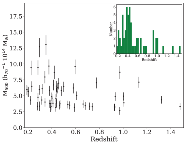
Figure 1: The distribution in SZE halo mass and redshift of the SPT-selected galaxy clusters observed with XMM-Newton is shown with each cluster appearing as a point with error bar. The inset shows the cluster redshift histogram.

We exclude clusters at $z<0.20$ from the scaling relation analysis, because their SZE mass estimates obtained via the $\zeta$–$M_{500}$ relation (Section 3.1) are impacted by the filtering adopted to remove signal from the primary CMB (see e.g., Benson et al., 2013). From this sample of 68 clusters, 59 are at redshift z$>$0.2 and have a total of 1000 or more filtered source counts in MOS observations and are therefore included in our final sample. The details of the XMM-Newton observations of these clusters are given in Table 2.2.

The final sample is shown in Figure 1 in redshift-mass space with an inset redshift histogram. This cluster sample is not a complete SZE signal-to-noise selected cluster sample. It has a median mass and redshift of $M_{500}=4.77\times 10^{14}M_{\odot}$ and $z_{\mathrm{med}}=0.45$, and five of the clusters lie at $z>1$. Nevertheless, the sample we study here has similar median mass, median redshift, and fraction of $z>1$ clusters as the SPT-SZ cosmology sample de Haan et al. (2016) , which has a median mass $M_{500}=4.57\times 10^{14}M_{\odot}$ (with roughly $6\%$ of the clusters at $z>1$), although it has a lower median redshift, 0.45 vs 0.55.

2.2 XMM-Newton Data Reduction

Our XMM-Newton data reduction is described in detail in Bulbul et al. (2012); here we summarize the main steps. XMM-Newton EPIC-MOS data analysis is carried out with Science Analysis System (SAS) version 16.0.0 and the latest available calibration files from Feb 2017. The Extended Source Analysis (ESAS) tools are used to reduce the data and extract the final data products (Snowden et al., 2008). The event files are filtered from the periods with elevated backgrounds through light-curve filtering. The good time interval files are produced and used to create cleaned event lists. The net exposure time after filtering the event lists for good time intervals is given in Table 2.2. There are three main detectors on board XMM-Newton: MOS1, MOS2, and PN. The back illuminated PN observations can be more sensitive to proton flares compared to MOS observations. As a result, the majority of the PN observation of some clusters in the sample is lost due to background filtering. Additionally, Schellenberger et al. (2015) reports up to a $54\%$ bias in temperature measurements between Chandra and PN temperature measurements in the soft 0.7–2 keV band where the bulk of detected photon flux from the high redshift clusters appears. To avoid creating potential biases in the X-ray observables, we only use MOS observations in this analysis. We examine the individual chips which may be affected by an anomalous background level and exclude them from further analysis (Kuntz & Snowden, 2008).

The images are created in the 0.5–2 keV band from the filtered event files and used to detect point sources within the MOS field-of-view (FOV). The images are examined carefully for point sources missed by the CIAO algorithm wavdetect. An exposure map is created for each MOS detector and each pointing to account for chip gaps and mirror vignetting. The quiescent particle background (QBP) image is created from the filter-wheel closed data as described in Snowden et al. (2008). The images and exposure maps of MOS1 and MOS2 detectors are combined prior to the background subtraction. The CIAO tool wavdetect convolved with the XMM-Newton’s point-spread-function (PSF) is used on the background-subtracted and exposure corrected images to detect point sources within the MOS FOV. All these point sources are excluded from further analysis.

We extract spectra using the ESAS tool mos-spectra within a radius of $R_{500}$ for each cluster (see Section 3 for the details of the $R_{500}$ calculation). Redistribution matrix files (RMFs) and ancillary response files (ARFs) are created with rmfgen and arfgen, respectively. QPB is subtracted from the total spectra prior to the fitting. The spectral fitting of the source is done in the spectral fitting package XSPEC 12.9.0 (Arnaud, 1996) with ATOMDB version 3.0.8 (Smith et al., 2001; Foster et al., 2012). The adopted solar abundances are from Lodders & Palme (2009). The Galactic Column density is allowed to vary within $15\%$ of the measured Kalberla et al. (2005) LAB value in our fits, following the approach described in McDonald et al. (2016). We use C-stat as a goodness of the fit estimator in XSPEC.

Spectra are extracted from two apertures of $<R_{500}$ and 0.15 $R_{500}$–$R_{500}$ (again, see Section 3 for discussion of $R_{500}$). The fits are performed in the 0.3–10 keV energy interval. The higher energy band 7–10 keV is used to constrain soft-proton contamination accurately. Soft-proton flares are largely removed by the light curve filtering. However, after the filtering some residuals may remain in the data. These are modeled by including an extra power-law model component to the total model and the MOS diagonal response matrices provided in the SAS distribution (Snowden et al., 2008). The cluster emission is fit with an absorbed single temperature apec model with free metallicity and temperature. Constraining metallicity is challenging for low-count observations of some of our high-z clusters. In these cases, we fixed the metallicity at 0.3$Z_{\odot}$, the typical value at both low and high redshifts (Tozzi et al., 2003).

Table 1: SPT clusters observed with XMM-Newton.

Name	z	Obs. ID	Exposure [ks]	Counts
			MOS1/MOS2	MOS1/MOS2
SPT-CLJ0114-4123	0.38	724770901	12.46 / 12.64	2350 / 2314
		404910201	16.31 / 16.78
SPT-CLJ0205-5829	1.32	675010101	55.86 / 57.14	1378 / 1299
SPT-CLJ0217-5245	0.34	652951401	8.91 / 14.52	1280 / 2052
SPT-CLJ0225-4155	0.22	692933401	12.40 / 11.92	7650 / 7257
SPT-CLJ0230-6028	0.68	675010401	19.37 / 22.72	875 / 921
SPT-CLJ0231-5403	0.59	204530101	17.38 / 22.17	719 / 843
SPT-CLJ0232-4421	0.28	423403010	11.59 / 12.09	7917 / 8183
SPT-CLJ0233-5819	0.66	675010601	49.14 / 50.01	2396 / 2370
SPT-CLJ0234-5831	0.42	674491001	12.53 / 13.47	2182 / 2333
SPT-CLJ0240-5946	0.40	674490101	14.38 / 14.03	1852 / 1733
SPT-CLJ0243-4833	0.50	672090501	9.80 / 9.74	2078 / 2002
		723780801	12.40 / 11.31
SPT-CLJ0254-5857	0.44	656200301	11.62 / 13.17	3145 / 3501
		674380300	11.62 / 13.17
SPT-CLJ0254-6051	0.44	692900201	16.01 / 15.65	1516 / 1399
SPT-CLJ0257-5732	0.43	674491101	27.31 / 27.95	886 / 859
SPT-CLJ0304-4401	0.46	700182201	16.57 / 16.75	3439 / 3429
SPT-CLJ0317-5935	0.47	674490501	7.83 / 10.82	1615 / 1572
		724770401	14.73 / 14.80
SPT-CLJ0330-5228	0.44	400130101	69.12 / 67.81	24535 / 24023
SPT-CLJ0343-5518	0.55	724770801	17.91 / 18.03	988 / 918
SPT-CLJ0344-5452	1.00	675010701	48.74 / 48.94	769 / 735
SPT-CLJ0354-5904	0.41	724770501	14.19 / 16.87	1669 / 1931
SPT-CLJ0403-5719	0.46	674491201	18.40 / 19.94	1900 / 1977
SPT-CLJ0406-5455	0.74	675010501	53.25 / 55.69	1611 / 1646
SPT-CLJ0417-4748	0.58	700182401	21.86 / 23.39	2590 / 2736
SPT-CLJ0438-5419	0.42	656201601	17.87 / 17.87	4904 / 4857
SPT-CLJ0510-4519	0.20	692933001	12.80 / 13.05	7838 / 7901
SPT-CLJ0516-5430	0.29	205330301	10.41 / 10.67	14848 / 14812
		692934301	26.94 / 26.97
SPT-CLJ0522-4818	0.29	303820101	11.57 / 15.00	2631 / 3314
SPT-CLJ0549-6205	0.37	656201301	13.17 / 13.00	7835 / 7688
SPT-CLJ0559-5249	0.61	604010301	16.64 / 17.39	1800 / 1756
SPT-CLJ0611-5938	0.39	658201101	12.91 / 13.18	1629 / 1591
SPT-CLJ0615-5746	0.97	658200101	12.59 / 13.31	1587 / 1613
SPT-CLJ0637-4829	0.20	692933101	- / 11.81	6643 / 5859
SPT-CLJ0638-5358	0.23	650860101	24.77 / 31.65	21985 / 27911
SPT-CLJ0658-5556	0.29	112980201	21.50 / 21.66	26213 / 26326
SPT-CLJ2011-5725	0.28	744390401	17.07 / 17.53	3981 / 4065
SPT-CLJ2017-6258	0.53	674491501	25.43 / 25.42	1428 / 1322
SPT-CLJ2022-6323	0.38	674490601	14.33 / 14.21	2129 / 2015
SPT-CLJ2023-5535	0.23	069293370	2.93 / 4.31	1942 / 2627
SPT-CLJ2030-5638	0.39	724770201	20.82 / 21.05	1393 / 1447
SPT-CLJ2031-4037	0.34	690170701	10.25 / 10.20	3553 / 3447
SPT-CLJ2032-5627	0.28	674490401	24.67 / 25.32	10032 / 10221
SPT-CLJ2040-5725	0.93	675010201	75.08 / 76.75	1916 / 1919
SPT-CLJ2040-4451	1.48	723290101	75.96 / 75.37	844 / 775
SPT-CLJ2056-5459	0.72	675010901	40.11 / 39.58	1060 / 990
SPT-CLJ2106-5844	1.13	744400101	39.10 / 45.70	3035 / 3501
SPT-CLJ2109-4626	0.97	694380101	52.36 / 55.57	713 / 744
SPT-CLJ2124-6124	0.44	674490701	14.00 / 14.36	1365 / 1416
SPT-CLJ2130-6458	0.31	069290010	6.3 / 8.5	1108 / 1450
SPT-CLJ2131-4019	0.45	724770601	12.50 / 12.73	2598 / 2600
SPT-CLJ2136-6307	0.93	675010301	56.68 / 59.69	2465 / 2499
SPT-CLJ2138-6008	0.32	674490201	12.80 / 14.12	2918 / 3253
SPT-CLJ2145-5644	0.48	674491301	10.12 / 10.65	1442 / 1443
SPT-CLJ2146-4633	0.93	744401301	70.40 / 74.13	2370 / 2434
		744400501	93.33 / 96.20
SPT-CLJ2200-6245	0.39	724771001	9.55 / 10.53	623 / 631
SPT-CLJ2248-4431	0.35	504630101	25.23 / 26.25	24646 / 25604
SPT-CLJ2332-5358	0.40	604010101	6.82 / 6.82	1434 / 1443
SPT-CLJ2337-5942	0.77	604010201	18.36 / 19.32	1893 / 1952
SPT-CLJ2341-5119	1.00	744400401	72.63 / -	2788 / 3145
SPT-CLJ2344-4243	0.59	722700101	108.58 / 110.77	32697 / 33314
		722700201	87.18 / 87.01
		693661801	12.96 / 13.44

We also consider the X-ray foreground emission, including Galactic halo, local hot bubble, cosmic X-ray background due to unresolved extragalactic sources, and solar wind charge exchange. The ROSAT All-Sky Survey background spectra extracted beyond $R_{\mathrm{vir}}$ (discussed in Section 3) are used to model the soft X-ray background as described in Bulbul et al. (2012). The soft X-ray emission from the local hot bubble is modeled with a cool unabsorbed apec component with kT$\approx$0.1 keV, abundance of $Z_{\odot}$ at $z=0$, while the Galactic halo is modeled with a warmer absorbed thermal component kT$\approx$0.25 keV, abundance of $Z_{\odot}$ at $z=0$. The temperatures of the apec models are restricted, but the normalizations are allowed to vary in our fits. We model the cosmic X-ray background due to unresolved point sources using an absorbed power-law component with a spectral index of 1.4 (Hickox & Markevitch, 2005) and normalization of $\approx$9$\times 10^{-7}$ photons keV^-1 cm^-2 s^-1 at $\approx$1 keV (Kuntz & Snowden, 2008; Moretti et al., 2003). The bright instrumental fluorescent lines Al–K (1.49 keV) and Si–K (1.74 keV) are not included in the MOS QBP files. Therefore, we model these instrumental lines by adding Gaussian models to our spectral fits to determine the best-fit energies, and normalizations.

Because of scattering in the XMM-Newton mirrors, some of the flux that originates from one area of the sky is detected in a different area of the detector. This is not a major concern if the gradient in plasma temperature from core to outskirts is smooth; however, it may be important for clusters with a strong cool core. Additionally, for high redshift clusters, 0.15 $R_{500}$ (discussed in Section 3) is comparable to the PSF for XMM-Newton, so this PSF effect is crucial and must be accounted for when making spectral fits. This radial cross-talk or contamination effect is treated as an additional model component in XSPEC. The cross-talk ARFs for the contribution of X-rays originating from a region on the sky to the another region on the detector are created using the SAS tool arfgen (Snowden et al., 2008). The cross-talk correction is applied to eliminate PSF effects for all clusters in our sample.

3 Cluster Masses and X-ray Observables

The relationship between cluster X-ray observables (including emission-weighted mean temperature ${T_{\mathrm{X}}}$, integrated pressure $Y_{\mathrm{X}}$, ICM mass $M_{\mathrm{ICM}}$ and luminosity $L_{\mathrm{X}}$) and halo mass and cluster redshift exhibit a low scatter outside of the cluster center, where non-gravitational effects such as heating and cooling processes are less important (Fabian et al., 1994; Mohr & Evrard, 1997; O’Hara et al., 2006; Kravtsov et al., 2005; Nagai et al., 2007). We, therefore, measure all the X-ray observables both with and without the core region (except for the ICM mass $M_{\mathrm{ICM}}$ where the core has no impact). Specifically, we extract observables within an aperture (0.15–1)$R_{500}$ (core-excised marked as $cex$) and (0–1)$R_{500}$ (core-included marked as $cin$). The cluster radius $R_{500}$ is determined using the SZE-based halo mass $M_{500}$ using

$$R_{500}=\left(\frac{3M_{500}}{4\pi\times 500\rho_{\mathrm{crit}}(z)}\right)^{1/3},$$ (1)

where the $M_{500}$ masses are described in the next section, and $\rho_{\mathrm{crit}}(z)$ is the critical density of the Universe at the cluster redshift.

3.1 SZE-based mass $M_{500}$

We derive the cluster mass $M_{500}$ based on the SZE signal-to-noise ratio $\xi$ and redshift $z$ as determined by SPT. The measured signal-to-noise $\xi$ is a biased observable subject to Gaussian noise that is extracted through a matched filter approach that employs a $\beta$ model with three degrees of freedom: sky location ($\alpha,\delta$) and core-radius $\theta_{\mathrm{C}}$. The mean value of the signal-to-noise $\left\langle\xi\right\rangle$ is related to the underlying unbiased signal-to-noise $\zeta$ as follows.

$$\left\langle\xi\right\rangle=\sqrt{\zeta^{2}+3}\,,$$ (2)

for $\zeta>2$ (de Haan et al., 2016). The $\zeta$–mass scaling relation is parametrized as follows:

$$\zeta=A_{\mathrm{SZ}}\left(\frac{M_{500}}{4.3\times 10^{14}M_{\odot}}\right)^{B_{\mathrm{SZ}}}\left(\frac{E(z)}{E(z_{\mathrm{piv}})}\right)^{C_{\mathrm{SZ}}}\,,$$ (3)

where the normalization is $A_{\mathrm{SZ}}$, the mass trend parameter is $B_{\mathrm{SZ}}$, the redshift trend parameter is $C_{\mathrm{SZ}}$, and there is log-normal intrinsic scatter in the observables at fixed mass of $\sigma_{\ln\zeta}$.

In this work we marginalize over the parameters of the $\zeta$–mass relation while fitting the parameters of the X-ray scaling relations that are investigated. This ensures that the final uncertainties in the X-ray observable–mass–redshift scaling relations include the systematic uncertainties associated with the imperfectly known SZE-based halo masses. In the interest of focusing on the X-ray scaling relations, we adopt priors on the parameters of the $\zeta$–mass relation that correspond to the fully marginalized posterior distributions reported in de Haan et al. (2016) (Table 2). This approach does not capture any covariances among the $\zeta$–mass scaling relation parameters, but these are indeed small (see de Haan et al., 2016, Figure 5). The advantage is that the likelihood we must calculate in each iteration of the Markov chain involves our X-ray observables and the simple priors on the SZE $\zeta$–mass relation parameters.

Table 2: Gaussian priors $\mathcal{N}(\mu,\sigma^{2})$ on the SZE observable-mass relation parameters appear first followed by uniform priors $\mathcal{U(\mathrm{min},\mathrm{max})}$ on the X-ray observable–mass relation parameters.

Parameters	Priors
SZE $\zeta-M_{500}-z$ parameters
$A_{\mathrm{SZ}}$	$\mathcal{N}(4.842,0.913^{2})$
$B_{\mathrm{SZ}}$	$\mathcal{N}(1.668,0.083^{2})$
$C_{\mathrm{SZ}}$	$\mathcal{N}(0.550,0.315^{2})$
$\sigma_{\ln\zeta}$	$\mathcal{N}(0.199,0.069^{2})$
X-ray $\mathcal{X}-M_{500}-z$ parameters
$A_{{T_{\mathrm{X}}}}$	$\mathcal{U}(0.1,20)$ keV
$A_{M_{\mathrm{ICM}}}$	$\mathcal{U}(10^{12},2\times 10^{14})$ $M_{\odot}$
$A_{Y_{\mathrm{X}}}$	$\mathcal{U}(5\times 10^{12},2\times 10^{15})$ keV$M_{\odot}$
$A_{L_{\mathrm{X}}}$	$\mathcal{U}(2\times 10^{43},1.2\times 10^{45})$ ergs s-1
$B_{\mathcal{X}}$	$\mathcal{U}(0.1,3.5)$
$C_{\mathcal{X}}$	$\mathcal{U}(-4,4)$
$\sigma_{\ln\mathcal{X}}$	$\mathcal{U}(0.005,1.5)$
$\gamma_{\mathcal{X}}$	$\mathcal{U}(-4,4)$
$\delta_{\mathcal{X}}$	$\mathcal{U}(-4,4)$

The priors we adopt on the SZE observable mass relation are shown in Table 2, where $\mathcal{N}(\mu,\sigma^{2})$ corresponds to a Gaussian with mean $\mu$ and dispersion $\sigma$. These SZE $\zeta$–mass parameter constraints emerge from a joint cosmology and mass calibration analysis that uses as input: (1) the SPT cluster distribution in $\xi$ and z (i.e. the number counts), (2) mass information from externally weak lensing calibrated $Y_{\mathrm{X}}$ measurements for 82 systems, and (3) external cosmological parameter constraints (for more extensive discussion of SPT mass calibration see, e.g., Bocquet et al., 2015; Chiu et al., 2018). For the baseline priors listed above, the external cosmological priors include a prior on the Hubble parameter (Riess et al., 2011) and a prior on the baryon density parameter from Big Bang Nucleosynthesis (Cooke et al., 2014).

Although the mass calibration presented in de Haan et al. (2016) includes information from Chandra X-ray observations of 82 clusters, we stress that the mass information is dominated by the cluster distribution in $\xi$ and redshift (i.e., the halo mass function information). That is, the $\zeta-$mass$-$redshift relation used to calculate SPT-SZ masses does not simply follow the employed $Y_{\mathrm{X}}-$mass$-$redshift relation, because it is a subdominant component of the mass information. Moreover, we adopt the resulting posteriors of the $\zeta-$mass relation as the priors in this work, effectively marginalizing over the systematic uncertainties of all ingredients used in calibrating the cluster mass. Modeling these priors as independent Gaussian distributions is appropriate, given the lack of strong covariances in the joint parameter constraints presented in de Haan et al. (2016, see Figure 5). It is important to note that the correlated intrinsic scatter between the mass proxies of SZE and X-ray does not impact the mass calibration with the current sample size (de Haan et al., 2016; Dietrich et al., 2017), therefore, we can use the existing $\zeta-$mass$-$redshift relation with marginalized systematic uncertainties to investigate the X-ray observable-to-mass scaling relations.

To foreshadow an additional set of results that we present, we also adopt a separate set of priors derived from the second results column of Table 3 in de Haan et al. (2016), which include also an external cosmological prior coming from BAO distance measurements (Anderson et al., 2014). This set of results is consistent with the baseline results, but has smaller uncertainties (because the cosmological uncertainties typically dominate the posterior distributions of the SZE $\zeta$–mass parameters) and has a shift of $\Delta C_{\mathrm{SZ}}=+0.3$ that translates into a corresponding shift in the redshift trend parameters in the X-ray scaling relations.

Because we adopt similar four-parameter scaling relations for both the SZE and X-ray observables, we denote the targeted X-ray scaling relation (e.g., equation 10) as $r_{\mathcal{X}}=(A_{\mathcal{X}},B_{\mathcal{X}},C_{\mathcal{X}},\sigma_{\ln\mathcal{X}})$ and the one used for estimating $M_{500}$ as $r_{\zeta}=(A_{\mathrm{SZ}},B_{\mathrm{SZ}},C_{\mathrm{SZ}},\sigma_{\ln\zeta})$. The notation $r_{\mathcal{X}}$ can be similarly extended to the five-parameter scaling relations for the X-ray observables, for which we define the functional forms in Section 4.1.

We stress that the cluster masses in our work include corrections for selection biases (e.g. the Eddington bias, the Malmquist bias) and therefore they reflect the unbiased distribution of cluster mass $M_{500}$ given the observable $\xi$ and redshift $z$ measured for each SZE-selected cluster.

Table 3: Measurements of the X-ray observables and cluster masses.

Note. — X-ray observables of the sample measured in core-included ($\mathrm{cin}$, $r<R_{500}$) and core-excised ($\mathrm{cex}$, $0.15R_{500}<r<R_{500}$) apertures. Parameters marked with ^∗ are fixed to the indicated values. From left to right is the cluster name, $R_{500}$, bolometric and soft-band luminosity, emission-weighted mean temperature and metallicity, given first for the core-included and then for the core-excised measurements. Measured ICM masses $M_{\mathrm{ICM}}$, X-ray derived integrated Compton-$y$ $Y_{\mathrm{X,cin}}$, and halo mass $M_{500}$ determined from the SZE observations are then listed for each cluster.

3.2 X-ray Observables

We measure the temperature, metallicity, and luminosity by fitting the spectra extracted in the apertures of the core-included region ($cin$, $r<R_{500}$) and core-excised region ($cex$, $0.15R_{500}<r<R_{500}$) with a single temperature thermal apec  model. The best-fit core-included temperatures (${T_{\mathrm{X,cin}}}$), metallicity ($Z_{\mathrm{X,cin}}$), and luminosities ($L_{\mathrm{X,cin}}$) and core-excised temperatures (${T_{\mathrm{X,cex}}}$), metallicity ($Z_{\mathrm{X,cex}}$), and luminosities ($L_{\mathrm{X,cex}}$) are given in Table 3.1. In some clusters, the statistics of the observations are too poor to allow a determination of the global metallicity. In these cases, the metallicity is fixed to $0.3Z_{\odot}$ (Tozzi et al., 2003; McDonald et al., 2016). The metallicity constraints, and their evolution with redshift in this sample is extensively discussed in McDonald et al. (2016).

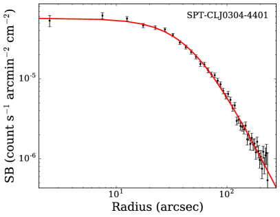
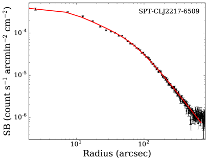
Figure 2: XMM-Newton MOS surface brightness profile of a non-cool core cluster SPT-CL J0304$-$4401 (left) and a cool-core cluster SPT-CL J0403$-$5719 (right). The red line shows the best-fit models convolved with the XMM-Newton PSF.

The X-ray surface brightness is extracted from background-subtracted, exposure-corrected images within 1.5$R_{500}$ in the fitting environment Sherpa in CIAO (Freeman et al., 2001; Doe et al., 2007). We fit a 2-dimensional $\beta$ profile to determine the cluster centroids within software package Sherpa. This method also allows for precise measurements of X-ray centroids of the clusters in the sample. The X-ray surface brightness $S_{\mathrm{X}}$ (in units of erg s^-1 cm^-2 steradian^-1), produced by thermal Bremsstrahlung and line emission, is expressed as

$$S_{\mathrm{X}}=\frac{1}{4\pi(1+z)^{4}}\int n_{\mathrm{e}}n_{\mathrm{H}}\Lambda_{\mathrm{eH}}(T_{\mathrm{X}},Z)\ dl,$$ (4)

where $\Lambda_{\mathrm{eH}}(T_{\mathrm{X}},Z)$ is the band averaged emissivity which is dependent on plasma temperature and metallicity, $dl$ is the integral along the line of sight, and $z$ is the cluster redshift. The electron and Hydrogen number densities ($n_{\mathrm{e}}$ and $n_{\mathrm{H}}$) have only weak dependence on plasma temperature and assumed abundance when derived from surface brightness in the 0.5–2 keV band (Mohr et al., 1999).

We fit the surface brightness profiles using an analytic density model (Bulbul et al., 2010, Bu10 hereafter):

$$n_{\mathrm{e}}(r)=n_{\mathrm{e}0}\left(\frac{1}{\left(\beta-2\right)}\frac{(1+r/r_{\mathrm{s}})^{\beta-2}-1}{r/r_{\mathrm{s}}(1+r/r_{\mathrm{s}})^{\beta-2}}\right)^{n}$$ (5)

where $n_{\mathrm{e}0}$ is the normalization of the electron density profile, $r_{\mathrm{s}}$ is the scale radius, $n$ is the slope of the density profile, and $\beta$ is the slope of the dark matter potential. We assume that the dark matter halos of the SPT selected sample follows the Navarro-Frenk-White (NFW) profile with a slope of $\beta=2$ (Navarro et al., 1997) and provides a good description of the electron density (Bu10; Bonamente et al., 2012). Application of the L’Hospital rule gives an electron density profile under the assumption of a NFW-like matter profile,

$$n_{\mathrm{e}}(r)=\tau_{\mathrm{cool}}(r)\ n_{\mathrm{e}0}\left(\frac{\ln(1+r/r_{\mathrm{s}})}{r/r_{\mathrm{s}}}\right)^{n}.$$ (6)

The Bu10 density profile has been used for fitting both X-ray and SZE data (Landry et al., 2013; Romero et al., 2017). The core taper function $\tau_{\mathrm{cool}}(r)$ is used to fit the surface brightness profiles of cool-core clusters (Vikhlinin et al., 2006)

$$\tau_{\mathrm{cool}}(r)=\frac{\alpha+(r/r_{\mathrm{cool}})^{\gamma}}{1+(r/r_{\mathrm{cool}})^{\gamma}}$$ (7)

For non-cool core clusters the parameter $\alpha$ is set to 1.

The Bu10 density model is projected along the line-of-sight and fit to the surface brightness profile obtained from background subtracted and exposure corrected X-ray images. The fitting is performed using a Markov chain Monte Carlo (MCMC) sampler within the emcee package in python (Foreman-Mackey et al., 2013). The best-fit parameter values and their 1$\sigma$ uncertainties for non-cool core clusters (e.g., $n_{\mathrm{e}0}$, $n$, $r_{\mathrm{s}}$) and cool-core clusters (e.g., $n_{\mathrm{e}0}$, $n$, $\alpha$, $r_{\mathrm{s}}$, and $r_{cool}$) are determined using a maximum likelihood method. The surface brightness profile fit to the MOS observations of a non-cool core cluster SPT-CL J0304$-$4401 and a cool-core cluster SPT-CL J2217$-$6509 are shown in Figure 2.

To compute the ICM mass of a cluster within a given aperture of $R_{500}$, we use the enclosed ICM mass obtained by integrating the best-fit 3D ICM density profile,

$$M_{\mathrm{ICM}}=4\pi\mu_{\mathrm{e}}m_{\mathrm{p}}\int_{0}^{R_{500}}n_{\mathrm{e}}(r)\ r^{2}\ dr,$$ (8)

where $\mu_{\mathrm{e}}$ is the mean molecular weight of the electrons, and $m_{\mathrm{p}}$ is the proton mass. The ICM mass measurements within $R_{500}$ for each cluster in the sample are given in Table 3.1. We use $\mu_{\mathrm{e}}=1.17$ when determining the cluster ICM mass. The integrated Compton-$y$ parameter is the product of the ICM mass and temperature

$$Y_{\mathrm{X}}=M_{\mathrm{ICM}}\times{T_{\mathrm{X}}}\,,$$ (9)

where ${T_{\mathrm{X}}}$ is the projected temperature measured within a 2D aperture either with or without the core and $M_{\mathrm{ICM}}$ is integrated within a 3D sphere of radius $R_{500}$.

As described already in Section 3.1, there are remaining uncertainties in the SZE-based halo masses. This means that the extraction radius $R_{500}$  used above is not a single value for each cluster, but a distribution of values. To include these uncertainties, we marginalize over them when studying the X-ray scaling relations. As described in Section 4.3, this means that we evaluate the X-ray observable at a range of radii $R_{500}$ consistent with the SZE observable $\xi$ and redshift $z$. Specifically, we use the best-fit density profile to calculate the ICM mass in each fit iteration. For $L_{\mathrm{X}}$ we extract the X-ray luminosity at a single radius—the baseline $R_{500}$—in this work, because we find the change in $L_{\mathrm{X}}$ due to the radial range in the surface brightness fit is negligible. For ${T_{\mathrm{X}}}$ we have in general too few photons to make spectral fits beyond the baseline $R_{500}$, and so we adopt only a single radius for the temperature extraction. This means that for $Y_{\mathrm{X}}$ we are properly including the variation of the $M_{\mathrm{ICM}}$ component with $R_{500}$ but not the ${T_{\mathrm{X}}}$ component.

4 Scaling Relation Form and Fitting

Self-similar models, based on gravitational collapse in clusters, predict simple power-law relations between cluster properties (Kaiser & Silk, 1986) that have been observed (using, e.g., ICM temperature, luminosity, ICM mass, X-ray isophotal size and total halo mass; Smith et al., 1979; Mushotzky & Scharf, 1997; Mohr & Evrard, 1997; Mohr et al., 1999; Arnaud & Evrard, 1999). As previously noted, the observed scaling relations often depart from self-similiar behavior, and this has been interpreted as evidence of feedback into the ICM from star formation and AGN as well as radiative cooling in the cluster cores.

In this section, we describe how we determine the best-fit parameters of the X-ray observable–halo mass–redshift scaling relations for the sample of 59 SPT selected galaxy clusters observed with XMM-Newton at $0.2<z<1.5$.

4.1 Three Forms of each Scaling Relation

We use three functional forms to characterize the X-ray observable–mass–redshift scaling relations. In all cases, there are pivot masses and redshifts that should be chosen to be near the median values of the sample to reduce artificial covariances between the amplitude parameter and the mass and redshift trend parameters. For the X-ray observable $\mathcal{X}$ to mass scaling relations, the pivot mass and pivot redshift are $M_{\mathrm{piv}}=6.35\times 10^{14}M_{\odot}$ and $z_{\mathrm{piv}}=0.45$, respectively.

The first form, similar to that used in Vikhlinin et al. (2009a) and many publications since, is defined as follows:

$$\mathcal{X}=A_{\mathcal{X}}\left(\frac{M_{500}}{M_{\mathrm{piv}}}\right)^{B_{\mathcal{X}}}\left(\frac{E(z)}{E(z_{\mathrm{piv}})}\right)^{C_{\mathcal{X}}},$$ (10)

where the normalization and trend parameters in mass and redshift are $A_{\mathcal{X}}$, $B_{\mathcal{X}}$ and $C_{\mathcal{X}}$, respectively, for the observable $\mathcal{X}$. Note that the redshift trend in this formulation is expressed as a function of the Hubble parameter $H(z)=H_{0}E(z)$, where $E^{2}(z)=\Omega_{\mathrm{M}}(1+z)^{3}+\Omega_{\Lambda}$ at late times in a flat $\Lambda$CDM Universe. That is, in this parametrization, the redshift evolution of the X-ray observable–mass relation is attributed an explicit cosmological dependence. In the case where the redshift evolution has a different cosmological dependence than adopted here (e.g., the evolution is non-self similar), then assuming this form will lead to biases in cosmological analyses. We refer to equation (10) as Form I hereafter.

The second form includes the expected self-similar evolution of the observable with redshift, which depends on the cosmologically dependent evolution of the critical density, while modeling departures of the observable from self-similar evolution with a function $(1+z)^{\gamma_{\mathcal{X}}}$. With this form we are adopting the view that the departures from self-similar evolution do not have a clearly understood cosmological dependence. Therefore, we model the departures with the cosmologically agnostic form $(1+z)^{\gamma_{\mathcal{X}}}$ that has been adopted in many previous works (e.g. Lin et al., 2006). This form is defined as follows:

$$\mathcal{X} = A_{\mathcal{X}}\left(\frac{M_{500}}{M_{\mathrm{piv}}}\right)^{B_{\mathcal{X}}}\left(\frac{E(z)}{E(z_{\mathrm{piv}})}\right)^{C_{\mathrm{\mathcal{X},SS}}}\left(\frac{1+z}{1+z_{\mathrm{piv}}}\right)^{\gamma_{\mathcal{X}}}$$ (11)

where the normalization and mass trend are similarly characterized by the parameters $A_{\mathcal{X}}$ and $B_{\mathcal{X}}$, respectively. The redshift trend is modeled with $C_{\mathrm{\mathcal{X},SS}}$ fixed to the self-similar expectation along with the factor $(1+z)^{\gamma_{\mathcal{X}}}$ to describe the departure of the redshift trend from the self-similar expectation. For instance, $C_{\mathrm{\mathcal{X},SS}}=\frac{2}{3}$ for the X-ray temperature–mass–redshift relation. In this way, the parameter $\gamma_{\mathcal{X}}$ directly quantifies the deviation from the self-similar redshift trend. This form of the scaling relation is easily distinguishable, because it has a parameter $\gamma_{\mathcal{X}}$ rather than $C_{\mathcal{X}}$. We refer to equation (11) as Form II hereafter.

The third form we adopt is much like Form II above, but it includes a cross-term between cluster mass and redshift to characterize the possibility of having a redshift-dependent mass trend. Specifically, the third functional form is

$$\mathcal{X} = A_{\mathcal{X}}\left(\frac{M_{500}}{M_{\mathrm{piv}}}\right)^{B^{\prime}_{\mathcal{X}}}\left(\frac{E(z)}{E(z_{\mathrm{piv}})}\right)^{C_{\mathrm{\mathcal{X},SS}}}\left(\frac{1+z}{1+z_{\mathrm{piv}}}\right)^{\gamma_{\mathcal{X}}}$$ (12)

where the mass trend $B^{\prime}_{\mathcal{X}}=B_{\mathcal{X}}+\delta_{\mathcal{X}}\ln\left(\frac{1+z}{1+z_{\mathrm{piv}}}\right)$ has a characteristic value of $B_{\mathcal{X}}$ at the pivot redshift and an additional rate of variation $\delta_{\mathcal{X}}$ with redshift. The normalization parameter $A_{\mathcal{X}}$ and the redshift trend $\gamma_{\mathcal{X}}$ are defined as in Form II. Specifically, the redshift trend is structured to capture the departures from the expected self-similar redshift evolution of the X-ray observable. It is worth mentioning that $\delta_{\mathcal{X}}=0$ or statistically consistent with zero indicates there is no evidence for a redshift-dependent mass trend. We refer to equation (12) as Form III hereafter.

For all three functional forms, we adopt log-normal intrinsic scatter in the observable at fixed mass, defined as

$$\sigma_{\ln\mathcal{X}}\equiv\sigma_{\ln\left(\mathcal{X}|M_{500}\right)}.$$ (13)

In this way, each observable $\mathcal{X}$ to mass scaling relation is parametrized by either $(A_{\mathcal{X}},B_{\mathcal{X}},C_{\mathcal{X}},\sigma_{\ln\mathcal{X}})$, $(A_{\mathcal{X}},B_{\mathcal{X}},C_{\mathrm{\mathcal{X},SS}},\gamma_{\mathcal{X}},\sigma_{\ln\mathcal{X}})$ or $(A_{\mathcal{X}},B_{\mathcal{X}},C_{\mathrm{\mathcal{X},SS}},\gamma_{\mathcal{X}},\sigma_{\ln\mathcal{X}}$ δX), and we denote these parameter sets by $r_{\mathcal{X}}$ hereafter for simplicity. Note that the expected self-similar redshift evolution parameter $C_{\mathrm{\mathcal{X},SS}}$ is fixed, and so the first two parameterizations have four free parameters, and the last parametrization has five.

4.2 Fitting Procedure

We briefly introduce the likelihood and fitting framework below and refer the reader to previous publications for more details (Liu et al., 2015; Chiu et al., 2016c). This likelihood is designed to obtain the parameters of the targeted X-ray observable–mass–redshift scaling relation (e.g., $r_{\mathcal{X}}$) for a given sample that is selected using another observable (e.g., the SPT signal-to-noise $\xi$), for which the observable–mass–redshift relation is already known (e.g., equation (3) used in this work). Specifically, the $i$-th term in the likelihood $\mathcal{L}_{i}$ contains the probability of obtaining the X-ray observable $\mathcal{X}_{i}$ for the $i$-th cluster at redshift $z_{i}$ with SZE signal-to-noise $\xi_{i}$, given the scaling relations $r_{\mathcal{X}}$ and $r_{\mathcal{\xi}}$.

$$\begin{split}\mathcal{L}_{i}(r_{\mathcal{X}},r_{\zeta})&=P(\mathcal{X}_{i}|\xi_{i},z_{i},r_{\mathcal{X}},r_{\zeta})\\ &=\frac{\int\mathrm{d}M_{500}\ P(\mathcal{X}_{i},\xi_{i}|z_{i},r_{\mathcal{X}},r_{\zeta})\ n(M_{500},z_{i})}{\int\mathrm{d}M_{500}\ P(\xi_{i}|z_{i},r_{\mathcal{X}},r_{\zeta})\ n(M_{500},z_{i})}\,,\end{split}$$ (14)

where $n(M_{500},z_{i})$ is the mass function whose inclusion allows the Eddington bias correction to be included when determining the mass corresponding to the SZE observable $\xi$ at redshift $z$. The integrals are over the relevant range of the mass $M_{500}$ used in the mass function. The Tinker et al. (2008) mass function is used with fixed cosmological parameters in calculations of $n(M_{500},z_{i})$, although given the mass range of the SPT sample the use of a mass function determined from hydrodynamical simulations would make no difference (Bocquet et al., 2016).

We ignore correlated scatter between the X-ray observable $\mathcal{X}$ and SZE observable $\xi$ in our analysis. This will not impact our results, because in previous studies of the SPT-SZ sample no evidence of correlated scatter between the X-ray $Y_{\mathrm{X}}$, X-ray based $M_{\mathrm{ICM}}$ and the SZE signal-to-noise has emerged (de Haan et al., 2016; Dietrich et al., 2017). In future analyses with much larger X-ray samples, we plan to explore again the evidence for correlated scatter in the X-ray and SZE properties of the clusters. As discussed in Liu et al. (2015), in this limit of no correlated X-ray and SZE scatter, there are no selection effects to be accounted for in the X-ray scaling relation.

Based on Bayes’ Theorem, the best-fit scaling relation parameters $r_{\mathcal{X}}$ and $r_{\mathcal{X}}$ are obtained by maximizing the probability,

$$P(r_{\mathcal{X}},r_{\zeta})\propto\mathcal{L}(r_{\mathcal{X}},r_{\zeta})\mathcal{P}(r_{\mathcal{X}},r_{\zeta})\,,$$ (15)

where $\mathcal{P}(r_{\mathcal{X}},r_{\zeta})$ is the prior on $r_{\mathcal{X}}$ and $r_{\zeta}$ (see Table 2), and the likelihood $\mathcal{L}(r_{\mathcal{X}},r_{\zeta})$ is evaluated using equation (14) as follows.

$$\mathcal{L}(r_{\mathcal{X}},r_{\zeta})=\prod_{i=1}^{N_{\mathrm{cl}}}~{}\mathcal{L}_{i}(r_{\mathcal{X}},r_{\zeta})\,,$$ (16)

where $i$ runs over the $N_{\mathrm{cl}}$ clusters. We use the python package emcee to explore the parameter space. The intrinsic scatter and measurement uncertainties of $\xi_{i}$ for each cluster are taken into account while evaluating equation (16). We have verified that this likelihood recovers unbiased scaling relation parameters by testing it against large mocks ($>1300$ clusters). Moreover, it has been further optimized in the goal of obtaining the parameters of scaling relations in a high dimensional space (Chiu et al., 2016c).

We note that in each iteration of the chain we use the current value of $R_{500}$ for each cluster to recalculate the $M_{\mathrm{ICM}}$ (see Section 3.2). For the temperature ${T_{\mathrm{X}}}$ and the luminosity $L_{\mathrm{X}}$ we extract only once at the $R_{500}$ appropriate for the model $\zeta-M_{500}-z$ parameter values in our priors (see Table 2), because the impact of adjusting $R_{500}$ at each iteration is small.

4.3 Priors adopted during fitting

As discussed in Section 3.1, we marginalize over the parameters of the $\zeta$–$M_{500}$-$z$ while fitting the X-ray observable $\mathcal{X}$–$M_{500}$-$z$ relations (i.e., $r_{\zeta}$ and $r_{\mathcal{X}}$, respectively). Specifically, we adopt informative priors on $r_{\zeta}$, which have been obtained in a joint cosmology and mass calibration analysis described in (de Haan et al., 2016, see Table 3). Our baseline priors on $r_{\zeta}$ are listed in Table 2 and correspond to the posterior distributions for each parameter reported in the first results column of de Haan et al. (2016, Table 3 ). We explore a second set of priors on $r_{\zeta}$ corresponding to the posterior parameter distributions from the second results column of de Haan et al. (2016, Table 3), and we report those results in Table 5.

Our approach allows us to effectively marginalize over the remaining uncertainties in our $M_{500}$ estimates. In each iteration of the chain, each cluster has a different halo mass $M_{500}$ and associated radius $R_{500}$. The X-ray observables $M_{\mathrm{ICM}}$ and $Y_{\mathrm{X}}$ defined in Section 3.2 are then extracted at this radius $R_{500}$ and used to determine the likelihood for this iteration. Final uncertainties on the X-ray observable scaling relation parameters $r_{\mathcal{X}}$ therefore include not only those due to measurement uncertainties but also due to the (largely systematic) uncertainties in the underlying halo masses.

In the fitting, we apply the uniform priors listed in Table 2 on $r_{\mathcal{X}}$ during the likelihood maximization. With this approach we evaluate the scaling relations Form I, II, and III. In Table 2 we present the parameter in the first column and the form of the prior in column two. In this table $\mathcal{N}$ denotes a normal or Gaussian distribution, and $\mathcal{U}$ represents a uniform or flat distribution between the two values presented.

In a final step, we report the parameters of the Form III relation also while fixing the parameters of $r_{\zeta}$ to the best-fit values derived in de Haan et al. 2016 (i.e., the central values listed in Table 2). Through the comparison to the results when marginalizing over the posterior distributions with those when fixing the $r_{\zeta}$ parameters we can gauge the impact of the remaining systematic uncertainties on the SZE-based halo masses.

We note that the de Haan et al. (2016) priors we adopt when estimating cluster halo masses are derived using the cluster mass function information (distribution of clusters in signal-to-noise $\xi$ and $z$) together with a sample of 82 $Y_{\mathrm{X}}$ measurements that have been calibrated to mass first through hydrostatic masses (Vikhlinin et al., 2009a) and later through weak lensing (Hoekstra et al., 2015). We note that the mass information from the $Y_{\mathrm{X}}$ measurements is subdominant in comparison to that from the mass function information (see prior and posterior distributions on $r_{\mathcal{\xi}}$ parameters in Figure 5 of de Haan et al., 2016).

Moreover, the follow-up studies using weak lensing masses of 32 SPT-SZ clusters (Dietrich et al., 2017) and using dynamical masses from 110 SPT-SZ clusters (Capasso et al., 2017) have provided independent mass calibration of the $\zeta-M_{500}-z$ relation and cross-checks of cluster masses, and they are all in excellent agreement with the cluster masses in de Haan et al. (2016) as we adopt for our study. Ongoing work with DES weak lensing will further improve our knowledge of the $\zeta-M_{500}-z$ relation, allowing even more accurate cluster halo mass estimates in the future (e.g., Stern et al., 2018).

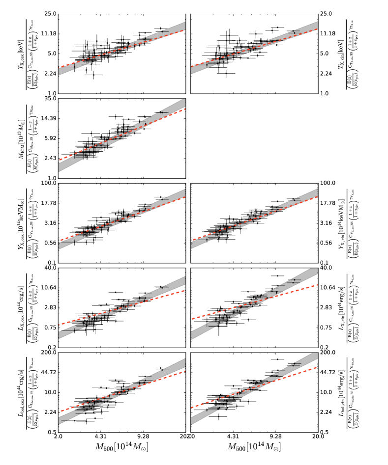
Figure 3: The power law trends of X-ray observables in mass corrected to the pivot redshift $z_{\mathrm{piv}}=0.45$ using the best-fit redshift trend from the Form II scaling relation (equation 11) for each observable. From top to bottom are ${T_{\mathrm{X}}}$, $M_{\mathrm{ICM}}$, $Y_{\mathrm{X}}$ and $L_{\mathrm{X}}$  with the core-excised observables (left) and included (right). The best-fit power law parameters and $1\sigma$ confidence intervals given in Table 4 are shown in the shaded region. For each row, the red dashed lines represent the best-fit normalizations at the pivotal mass with the mass scaling predicted by the self-similar trend in mass.

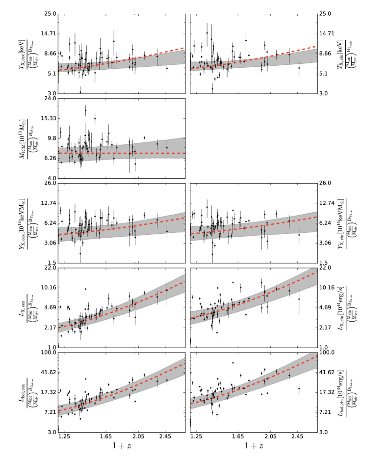
Figure 4: The power law trends of X-ray observables in redshift corrected to the pivot mass $M_{\mathrm{piv}}=6.35\times 10^{14}M_{\odot}$ using the best-fit mass trend from the Form II scaling relation (equation 11) for each observable. From top to bottom are ${T_{\mathrm{X}}}$, $M_{\mathrm{ICM}}$, $Y_{\mathrm{X}}$ and $L_{\mathrm{X}}$  with the core-excised observables (left) and included (right). The best-fit power law parameters and $1\sigma$ confidence intervals given in Table 4 are shown in the shaded region. For each row, the red dashed lines represent the best-fit normalizations at the pivotal mass with the redshift scaling predicted by the self-similar evolution.

Table 4: The best-fit parameters for the various X-ray observable–halo mass–redshift scaling relations. The first column contains the scaling relation identifier. Thereafter, the next six columns show best-fit parameters and associated fully marginalized $1\sigma$ uncertainties of the scaling relation normalization $A_{\mathcal{X}}$, mass trend $B_{\mathcal{X}}$, $E(z)$ redshift trend $C_{\mathcal{X}}$, log-normal intrinsic scatter $\sigma_{\ln\mathcal{X}}$, departure from self-similarity in redshift trend $(1+z)^{\gamma_{\mathcal{X}}}$ and redshift dependence $\delta_{\mathcal{X}}$ of the mass trend.

Scaling Relation	$A_{\mathcal{X}}$	$B_{\mathcal{X}}$	$C_{\mathcal{X}}$	$\sigma_{\ln\mathcal{X}}$	$\gamma_{\mathcal{X}}$	$\delta_{\mathcal{X}}$
$T_{\mathrm{X,cin}}-M_{500}-z$ Relation		$B_{\mathrm{\mathcal{X},SS}}={2\over 3}$	$C_{\mathrm{\mathcal{X},SS}}={2\over 3}$
I: $\mathcal{X}(M,z)\propto M_{500}^{B_{\mathcal{X}}}E(z)^{C_{\mathcal{X}}}$	$6.36^{+0.70}_{-0.64}$	$0.80\pm 0.10$	$0.33\pm 0.27$	$0.18\pm 0.04$	–	–
II: $\mathcal{X}(M,z)\propto M_{500}^{B_{\mathcal{X}}}E(z)^{2\over 3}(1+z)^{\gamma_{\mathcal{X}}}$	$6.41^{+0.64}_{-0.66}$	$0.79^{+0.08}_{-0.12}$	$2\over 3$	$0.18^{+0.05}_{-0.04}$	$-0.36^{+0.27}_{-0.26}$	–
III: as II with $B^{\prime}_{\mathcal{X}}=B_{\mathcal{X}}+\delta_{\mathcal{X}}\ln\left(\frac{1+z}{1+z_{\mathrm{piv}}}\right)$	$6.48^{+0.58}_{-0.69}$	$0.79^{+0.09}_{-0.10}$	$2\over 3$	$0.18^{+0.04}_{-0.04}$	$-0.22^{+0.29}_{-0.35}$	$0.81^{+0.56}_{-0.46}$
III with fixed SZE params	$6.41\pm 0.22$	$0.78^{+0.08}_{-0.09}$	$2\over 3$	$0.16^{+0.04}_{-0.03}$	$-0.20^{+0.23}_{-0.25}$	$0.77^{+0.57}_{-0.47}$
$T_{\mathrm{X,cex}}-M_{500}-z$ Relation		$B_{\mathrm{\mathcal{X},SS}}={2\over 3}$	$C_{\mathrm{\mathcal{X},SS}}={2\over 3}$
I: $\mathcal{X}(M,z)\propto M_{500}^{B_{\mathcal{X}}}E(z)^{C_{\mathcal{X}}}$	$6.17^{+0.71}_{-0.63}$	$0.83^{+0.09}_{-0.10}$	$0.28^{+0.28}_{-0.23}$	$0.13^{+0.05}_{-0.05}$	–	–
II: $\mathcal{X}(M,z)\propto M_{500}^{B_{\mathcal{X}}}E(z)^{2\over 3}(1+z)^{\gamma_{\mathcal{X}}}$	$6.09^{+0.76}_{-0.51}$	$0.80^{+0.11}_{-0.08}$	$2\over 3$	$0.13^{+0.04}_{-0.05}$	$-0.33^{+0.23}_{-0.28}$	–
III: as II with $B^{\prime}_{\mathcal{X}}=B_{\mathcal{X}}+\delta_{\mathcal{X}}\ln\left(\frac{1+z}{1+z_{\mathrm{piv}}}\right)$	$6.31^{+0.57}_{-0.69}$	$0.81^{+0.09}_{-0.08}$	$2\over 3$	$0.13^{+0.05}_{-0.04}$	$-0.30^{+0.27}_{-0.28}$	$0.35^{+0.53}_{-0.41}$
III with fixed SZE params	$6.17^{+0.20}_{-0.17}$	$0.79^{+0.10}_{-0.06}$	$2\over 3$	$0.12^{+0.04}_{-0.03}$	$-0.29^{+0.19}_{-0.25}$	$0.38^{+0.41}_{-0.43}$
$M_{\mathrm{ICM}}-M_{500}-z$ Relation		$B_{\mathrm{\mathcal{X},SS}}=1$	$C_{\mathrm{\mathcal{X},SS}}=0$
I: $\mathcal{X}(M,z)\propto M_{500}^{B_{\mathcal{X}}}E(z)^{C_{\mathcal{X}}}$	$6.80^{+1.09}_{-0.87}$	$1.260^{+0.10}_{-0.11}$	$0.17^{+0.28}_{-0.29}$	$0.12^{+0.04}_{-0.08}$	–	–
II: $\mathcal{X}(M,z)\propto M_{500}^{B_{\mathcal{X}}}E(z)^{0}(1+z)^{\gamma_{\mathcal{X}}}$	$7.37^{+0.76}_{-1.35}$	$1.26^{+0.12}_{-0.09}$	$0$	$0.10^{+0.04}_{-0.07}$	$0.18^{+0.30}_{-0.31}$	–
III: as II with $B^{\prime}_{\mathcal{X}}=B_{\mathcal{X}}+\delta_{\mathcal{X}}\ln\left(\frac{1+z}{1+z_{\mathrm{piv}}}\right)$	$7.09^{+0.91}_{-1.11}$	$1.26^{+0.11}_{-0.09}$	$0$	$0.10^{+0.05}_{-0.07}$	$0.16^{+0.33}_{-0.31}$	$0.16^{+0.47}_{-0.44}$
III with fixed SZE params	$7.02^{+0.21}_{-0.27}$	$1.26^{+0.09}_{-0.07}$	$0$	$0.07\pm 0.05$	$0.20^{+0.20}_{-0.22}$	$0.26^{+0.42}_{-0.51}$
$Y_{\mathrm{X,cin}}-M_{500}-z$ Relation		$B_{\mathrm{\mathcal{X},SS}}={5\over 3}$	$C_{\mathrm{\mathcal{X},SS}}={2\over 3}$
I: $\mathcal{X}(M,z)\propto M_{500}^{B_{\mathcal{X}}}E(z)^{C_{\mathcal{X}}}$	$4.70\pm 1.1$	$2.00^{+0.19}_{-0.14}$	$0.44^{+0.46}_{-0.54}$	$0.15^{+0.05}_{-0.12}$	–	–
II: $\mathcal{X}(M,z)\propto M_{500}^{B_{\mathcal{X}}}E(z)^{2\over 3}(1+z)^{\gamma_{\mathcal{X}}}$	$4.60\pm 1.1$	$1.99^{+0.17}_{-0.15}$	$2\over 3$	$0.16^{+0.05}_{-0.12}$	$-0.21^{+0.50}_{-0.45}$	–
III: as II with $B^{\prime}_{\mathcal{X}}=B_{\mathcal{X}}+\delta_{\mathcal{X}}\ln\left(\frac{1+z}{1+z_{\mathrm{piv}}}\right)$	$4.52^{+1.23}_{-0.91}$	$2.00^{+0.16}_{-0.17}$	$2\over 3$	$0.16^{+0.07}_{-0.10}$	$-0.28^{+0.56}_{-0.40}$	$0.77^{+0.74}_{-0.53}$
III with fixed SZE params	$4.57^{+0.25}_{-0.21}$	$1.98^{+0.16}_{-0.10}$	$2\over 3$	$0.07^{+0.09}_{-0.05}$	$-0.09^{+0.34}_{-0.32}$	$1.01^{+0.61}_{-0.71}$
$Y_{\mathrm{X,cex}}-M_{500}-z$ Relation		$B_{\mathrm{\mathcal{X},SS}}={5\over 3}$	$C_{\mathrm{\mathcal{X},SS}}={2\over 3}$
I: $\mathcal{X}(M,z)\propto M_{500}^{B_{\mathcal{X}}}E(z)^{C_{\mathcal{X}}}$	$4.31\pm 0.96$	$2.01^{+0.20}_{-0.13}$	$0.44\pm 0.49$	$0.16^{+0.04}_{-0.11}$	–	–
II: $\mathcal{X}(M,z)\propto M_{500}^{B_{\mathcal{X}}}E(z)^{2\over 3}(1+z)^{\gamma_{\mathcal{X}}}$	$4.50^{+1.0}_{-1.1}$	$2.02^{+0.16}_{-0.17}$	$2\over 3$	$0.11^{+0.07}_{-0.08}$	$-0.17^{+0.47}_{-0.50}$	–
III: as II with $B^{\prime}_{\mathcal{X}}=B_{\mathcal{X}}+\delta_{\mathcal{X}}\ln\left(\frac{1+z}{1+z_{\mathrm{piv}}}\right)$	$4.54^{+1.09}_{-0.98}$	$2.01^{+0.18}_{-0.14}$	$2\over 3$	$0.13^{+0.07}_{-0.08}$	$-0.20^{+0.52}_{-0.47}$	$0.55^{+0.78}_{-0.56}$
III with fixed SZE params	$4.40^{+0.23}_{-0.22}$	$2.04^{+0.10}_{-0.15}$	$2\over 3$	$0.04^{+0.08}_{-0.03}$	$-0.14^{+0.33}_{-0.32}$	$0.67^{+0.66}_{-0.74}$
$L_{\mathrm{X,cin}}-M_{500}-z$ Relation		$B_{\mathrm{\mathcal{X},SS}}={1}$	$C_{\mathrm{\mathcal{X},SS}}={2}$
I: $\mathcal{X}(z)\propto E(z)^{C_{\mathcal{X}}}$	$4.20^{+0.91}_{-0.92}$	$1.93^{+0.16}_{-0.20}$	$1.72^{+0.53}_{-0.46}$	$0.25^{+0.10}_{-0.10}$	–	–
II: $\mathcal{X}(z)\propto E(z)^{2}(1+z)^{\gamma_{\mathcal{X}}}$	$4.12^{+0.91}_{-0.94}$	$1.89^{+0.23}_{-0.13}$	$2$	$0.27^{+0.08}_{-0.12}$	$-0.20^{+0.51}_{-0.49}$	–
III: as II with $B^{\prime}_{\mathcal{X}}=B_{\mathcal{X}}+\delta_{\mathcal{X}}\ln\left(\frac{1+z}{1+z_{\mathrm{piv}}}\right)$	$4.39^{+0.82}_{-0.99}$	$1.93^{+0.19}_{-0.18}$	$2$	$0.28^{+0.07}_{-0.11}$	$-0.13^{+0.63}_{-0.46}$	$0.71^{+0.89}_{-0.72}$
III with fixed SZE params	$3.96^{+0.22}_{-0.24}$	$1.95^{+0.14}_{-0.18}$	$2$	$0.24^{+0.08}_{-0.06}$	$-0.02^{+0.32}_{-0.48}$	$0.84^{+0.81}_{-0.80}$
$L_{\mathrm{X,cex}}-M_{500}-z$ Relation		$B_{\mathrm{\mathcal{X},SS}}={1}$	$C_{\mathrm{\mathcal{X},SS}}={2}$
I: $\mathcal{X}(M,z)\propto M_{500}^{B_{\mathcal{X}}}E(z)^{C_{\mathcal{X}}}$	$2.84^{+0.60}_{-0.53}$	$1.60^{+0.17}_{-0.13}$	$1.86^{+0.47}_{-0.43}$	$0.27^{+0.07}_{-0.10}$	–	–
II: $\mathcal{X}(M,z)\propto M_{500}^{B_{\mathcal{X}}}E(z)^{2}(1+z)^{\gamma_{\mathcal{X}}}$	$2.84^{+0.53}_{-0.50}$	$1.60^{+0.16}_{-0.15}$	$2$	$0.27^{+0.07}_{-0.11}$	$-0.10^{+0.47}_{-0.42}$	–
III: as II with $B^{\prime}_{\mathcal{X}}=B_{\mathcal{X}}+\delta_{\mathcal{X}}\ln\left(\frac{1+z}{1+z_{\mathrm{piv}}}\right)$	$2.89^{+0.55}_{-0.51}$	$1.56^{+0.18}_{-0.16}$	$2$	$0.28^{+0.07}_{-0.08}$	$0.10^{+0.35}_{-0.60}$	$0.30^{+0.86}_{-0.62}$
III with fixed SZE params	$2.66^{+0.17}_{-0.11}$	$1.60^{+0.14}_{-0.16}$	$2$	$0.26^{+0.05}_{-0.05}$	$-0.01^{+0.33}_{-0.42}$	$0.60^{+0.79}_{-0.75}$
$L_{\mathrm{X,cin,bol}}-M_{500}-z$ Relation		$B_{\mathrm{\mathcal{X},SS}}={4\over 3}$	$C_{\mathrm{\mathcal{X},SS}}={7\over 3}$
I: $\mathcal{X}(M,z)\propto M_{500}^{B_{\mathcal{X}}}E(z)^{C_{\mathcal{X}}}$	$15.4^{+2.8}_{-3.3}$	$2.15^{+0.24}_{-0.19}$	$1.90^{+0.55}_{-0.53}$	$0.29^{+0.09}_{-0.13}$	–	–
II: $\mathcal{X}(M,z)\propto M_{500}^{B_{\mathcal{X}}}E(z)^{7\over 3}(1+z)^{\gamma_{\mathcal{X}}}$	$14.8^{+3.5}_{-2.7}$	$2.19^{+0.21}_{-0.17}$	$7\over 3$	$0.29^{+0.08}_{-0.13}$	$-0.14^{+0.62}_{-0.57}$	–
III: as II with $B^{\prime}_{\mathcal{X}}=B_{\mathcal{X}}+\delta_{\mathcal{X}}\ln\left(\frac{1+z}{1+z_{\mathrm{piv}}}\right)$	$13.8^{+3.2}_{-3.9}$	$2.12^{+0.23}_{-0.18}$	$7\over 3$	$0.31^{+0.08}_{-0.12}$	$-0.26^{+0.58}_{-0.60}$	$1.53^{+0.31}_{-1.11}$
III with fixed SZE params	$14.94^{+0.65}_{-1.01}$	$2.24^{+0.13}_{-0.15}$	$7\over 3$	$0.22^{+0.08}_{-0.10}$	$-0.17^{+0.43}_{-0.33}$	$1.67^{+0.28}_{-0.97}$
$L_{\mathrm{X,cex,bol}}-M_{500}-z$ Relation		$B_{\mathrm{\mathcal{X},SS}}={4\over 3}$	$C_{\mathrm{\mathcal{X},SS}}={7\over 3}$
I: $\mathcal{X}(M,z)\propto M_{500}^{B_{\mathcal{X}}}E(z)^{C_{\mathcal{X}}}$	$10.2^{+2.6}_{-2.1}$	$1.89^{+0.17}_{-0.18}$	$2.01^{+0.53}_{-0.44}$	$0.29^{+0.07}_{-0.12}$	–	–
II: $\mathcal{X}(M,z)\propto M_{500}^{B_{\mathcal{X}}}E(z)^{7\over 3}(1+z)^{\gamma_{\mathcal{X}}}$	$10.7\pm 2.3$	$1.88^{+0.19}_{-0.17}$	$7\over 3$	$0.27^{+0.07}_{-0.13}$	$-0.26^{+0.53}_{-0.43}$	–
III: as II with $B^{\prime}_{\mathcal{X}}=B_{\mathcal{X}}+\delta_{\mathcal{X}}\ln\left(\frac{1+z}{1+z_{\mathrm{piv}}}\right)$	$10.4^{+2.4}_{-2.2}$	$1.86^{+0.21}_{-0.16}$	$7\over 3$	$0.28^{+0.07}_{-0.09}$	$0.02^{+0.48}_{-0.58}$	$0.76^{+0.76}_{-0.71}$
III with fixed SZE params	$9.93^{+0.58}_{-0.49}$	$1.90^{+0.13}_{-0.18}$	$7\over 3$	$0.25^{+0.07}_{-0.06}$	$-0.18^{+0.48}_{-0.32}$	$0.80^{+0.93}_{-0.57}$

5 Scaling Relation Constraints

In this section, we describe the results of the fits and compare them to the self-similar expectation and to previous results in the literature. We present the scaling relations involving ${T_{\mathrm{X}}}$, then followed by $M_{\mathrm{ICM}}$, $Y_{\mathrm{X}}$ and $L_{\mathrm{X}}$. For all X-ray observables aside from $M_{\mathrm{ICM}}$ we present both core-included and -excised scaling relations.

Best-fit parameters and uncertainties are presented in Table 4, where the parameter constraints for each specific X-ray observable are presented in separate, delineated vertical subsections of the table. Within each table subsection the first line identifies the scaling relation and presents the self-similar expectation for the mass and redshift trends. Thereafter, the best-fit parameters are presented for the scaling relation Forms I, II, III and then III with fixed SZE scaling relation parameters. From left to right in the table we present the scaling relation and then the parameters for the normalization $A_{\mathcal{X}}$, mass trend $B_{\mathcal{X}}$, redshift trend $C_{\mathcal{X}}$ parametrized using $E(z)$, log-normal intrinsic scatter $\sigma_{\ln\mathcal{X}}$ of the observable at fixed $M_{500}$, departure from self-similar redshift scaling $\gamma_{\mathcal{X}}$, and redshift evolution of the mass trend $\delta_{\mathcal{X}}$.

5.1 $T_{\mathrm{X}}-M_{500}-z$ Relation

Before cluster mass measurements were available, the emission-weighted ICM temperature was viewed as the most robust mass proxy available and was therefore employed in early studies of cluster scaling relations (Smith et al., 1979; Mushotzky & Scharf, 1997; Mohr & Evrard, 1997; Mohr et al., 1999). Early attempts to constrain the ${T_{\mathrm{X}}}$–mass relation using hydrostatic masses were carried out first for low temperature clusters using spatially resolved spectroscopy from ROSAT (David et al., 1993) and then later for clusters with a broad range of temperature using the ASCA observatory (Finoguenov et al., 2001).

By combining the virial condition ($GM/R\sim T$) and the definition of the virial radius ($R_{500}\sim[M_{500}/\rho_{\mathrm{crit}}]^{1/3}$) one can show that the self similar expectation for the $T_{\mathrm{X}}-M_{500}-z$ relation is

$${T_{\mathrm{X}}}\propto{M_{500}}^{2/3}\ E(z)^{2/3}\,.$$ (17)

As noted in Section 4.2, we examine the scaling relations with and without the core region, and for three different scaling relation functional forms.

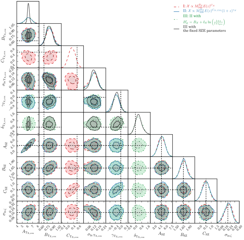
Figure 5: Parameter constraints on the core-excised $T_{\mathrm{X,cex}}-M_{500}-z$ relation. The parameter constraints while using Forms I, II, and III (see equations 10, 11 and 12) while adopting priors on the SZE mass-observable relation (see Table 2) are shown in red, blue and green, respectively. In addition, we show in black the results fitting of Form III while fixing the SZE scaling relation parameters to their best-fit values (de Haan et al., 2016). Fully marginalized constraints are shown on the diagonal, and—in the case of the X-ray parameters–are also presented in Table 4. The off-diagonal plots show joint constraints with $1\sigma$ and $2\sigma$ confidence contours. Parameters include the normalization $A_{{T_{\mathrm{X,cex}}}}$, power law index in mass $B_{{T_{\mathrm{X,cex}}}}$ and redshift $C_{{T_{\mathrm{X,cex}}}}$, deviation of the redshift trend from the self-similar prediction $\gamma_{{T_{\mathrm{X,cex}}}}$, the variation of the mass trend as a function of redshift $\delta_{{T_{\mathrm{X,cex}}}}$, and the intrinsic log-normal scatter in observable at fixed mass $\sigma_{\ln{T_{\mathrm{X,cex}}}}$. The parameters of the SZE observable–mass relation are the normalization $A_{\mathrm{SZ}}$, mass trend $B_{\mathrm{SZ}}$, redshift trend $C_{\mathrm{SZ}}$, and log-normal intrinsic scatter $\sigma_{\ln\zeta}$. The dashed lines mark self-similar expectation for the X-ray observable and best-fit values for the SZE mass–observable relation.

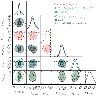
Figure 6: Similar to Figure  5 but containing constraints for the case of the core-included $T_{\mathrm{X,cin}}-M_{500}-z$ relation.

5.1.1 Parameter constraints

We present the parameters associated with the $T_{\mathrm{X,cin}}-M_{500}-z$ and $T_{\mathrm{X,cex}}-M_{500}-z$ relations relations in Table 4. The marginalized posteriors of the parameters and joint parameter confidence regions using the core-excised and -included observables are contained in Figures 5 and 6. Here we provide the best-fit $T_{\mathrm{X,cin}}-M_{500}-z$ and $T_{\mathrm{X,cex}}-M_{500}-z$ relations for the Form II scaling relation. For the core-included X-ray emission-weighted mean temperature,

$${T_{\mathrm{X,cin}}} = 6.41^{+0.64}_{-0.66}~{}\mathrm{keV}\left(\frac{M_{500}}{M_{\mathrm{piv}}}\right)^{0.80^{+0.09}_{-0.12}}$$ (18)

$$\left(\frac{E(z)}{E(z_{\mathrm{piv}})}\right)^{\frac{2}{3}}\left(\frac{1+z}{1+z_{\mathrm{piv}}}\right)^{-0.36^{+0.27}_{-0.26}},$$

with the intrinsic scatter of $0.18^{+0.05}_{-0.04}$. For the core-excised X-ray temperature ${T_{\mathrm{X,cex}}}$, the best-fit relation is

$${T_{\mathrm{X,cex}}} = 6.09^{+0.76}_{-0.51}~{}\mathrm{keV}\left(\frac{M_{500}}{M_{\mathrm{piv}}}\right)^{0.80^{+0.11}_{-0.08}}$$ (19)

$$\left(\frac{E(z)}{E(z_{\mathrm{piv}})}\right)^{\frac{2}{3}}\left(\frac{1+z}{1+z_{\mathrm{piv}}}\right)^{-0.33^{+0.23}_{-0.28}},$$

with intrinsic scatter of $0.13^{+0.05}_{-0.04}$. As for all relations, the mass and redshift pivots are $M_{\mathrm{piv}}=6.35\times 10^{14}M_{\odot}$ and $z_{\mathrm{piv}}=0.45$.

The mass trend parameters of the $T_{\mathrm{X,cex}}-M_{500}-z$ relations using forms I, II, and III (see equations 10, 11 and 12) are $0.83^{+0.09}_{-0.10}$, $0.80^{+0.11}_{-0.08}$ and $0.81^{+0.09}_{-0.08}$, respectively, showing consistency at better than the $1\sigma$ confidence level. All derived mass trends are consistent with the self-similar expectation at $\approx 1.6\sigma$ level. Note that there is neither a significant redshift-dependence in the mass trend ($\delta_{{T_{\mathrm{X,cex}}}}=0.35^{+0.53}_{-0.41}$) nor a strong deviation ($\gamma_{{T_{\mathrm{X,cex}}}}=-0.33^{+0.23}_{-0.28}$) from a self-similar redshift trend. In addition, as can be seen in Figure 5, there is a mild degeneracy between the slope and redshift evolution, such that the mass trend can be pushed back closer to the self-similar expectation with a stronger deviation of the redshift evolution from self-similarity. Fixing the SZE $\zeta$–mass relation does not change the best-fit parameters but reduces the uncertainty on the normalizations $A_{{T_{\mathrm{X}}}}$ by a factor of between two and three (see Table 4). This indicates that only the normalizations of the $T_{\mathrm{X}}-M_{500}-z$ relations are dominated by the systematic uncertainties in the SZE-based halo masses.

This behavior is clearly visible in Figure 5, where we show the joint confidence contours and fully marginalized posterior distributions for each of the $T_{\mathrm{X,cex}}-M_{500}-z$ relation variables for all three forms of the relation. In the figure, the self-similar parameter expectations are marked with dashed red lines. The preference for the mass trend to deviate by $\approx 2\sigma$ and the redshift trend to deviate by $\approx 1\sigma$ can be seen both in the joint parameter constraint panels and the fully marginalized single parameter distributions. Evidence for parameter covariance is clearest in the parameter pair $C_{T_{\mathrm{X,cex}}}$ and $\delta_{T_{\mathrm{X,cex}}}$. We include the four $\zeta-M_{500}-z$ relation parameters to show the strong positive correlations among the corresponding parameters $A_{\mathrm{SZ}}$ and $A_{T_{\mathrm{X,cex}}}$, $B_{\mathrm{SZ}}$ and $B_{T_{\mathrm{X,cex}}}$, $C_{\mathrm{SZ}}$ and $C_{T_{\mathrm{X,cex}}}$. Also a strong negative correlation among the scatter parameters $\sigma_{\ln\zeta}$ and $\sigma_{\ln{T_{\mathrm{X,cex}}}}$ are indicated by the same parameters. This is as expected and follows from the importance of the SZE-based masses in the $T_{\mathrm{X,cex}}-M_{500}-z$ relation and the fact that the quadrature sum of the scatter in $\zeta-M_{500}-z$ and $T_{\mathrm{X,cex}}-M_{500}-z$ is constrained by the measurement-error corrected scatter in the data about the best-fit $T_{\mathrm{X,cex}}-M_{500}-z$ relation. In all other cases that follow, we exclude the $\zeta-M_{500}-z$ parameters from the plots to conserve space, but the correlations persist, as expected. Finally, this plot makes clear (black lines) that the improvement from fixing the $\zeta-M_{500}-z$ scaling relation parameters at their best-fit values is a dramatic decrease in the uncertainties of $A_{T_{\mathrm{X,cex}}}$ but only a modest impact on the other parameters.

For the core-included $T_{\mathrm{X,cin}}-M_{500}-z$ relation, the mass and redshift trends as well as the normalization are consistent with those for the core-exclude case within the quoted $1\sigma$ uncertainties. The discernible difference in the two relations comes from intrinsic scatter. The log-normal intrinsic scatter for the core-excised observable at fixed mass $\sigma_{\ln{T_{\mathrm{X,cex}}}}$ is $\approx 0.12$, approximately a factor of 1.5 smaller than in the case of the core-included observable. Figure 6 contains the joint and single parameter constraints for this relation.

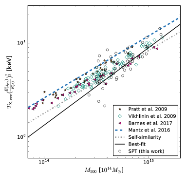
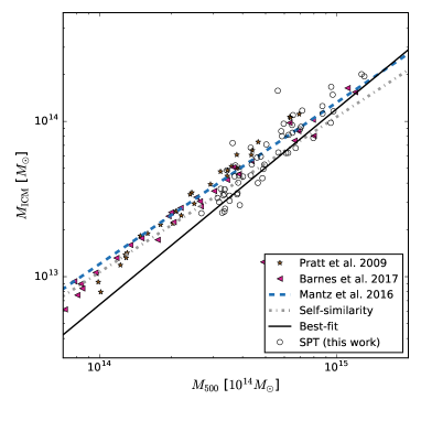
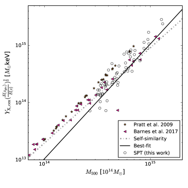
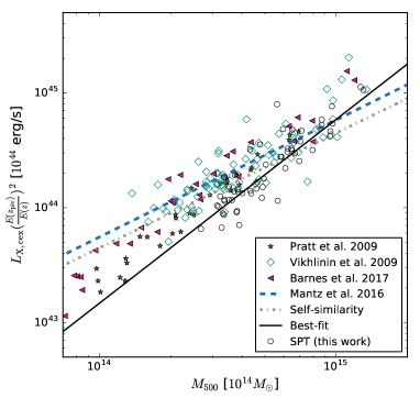
Figure 7: Core-excised soft band X-ray luminosity, core-excised ${T_{\mathrm{X}}}$, $M_{\mathrm{ICM}}$ and $Y_{\mathrm{X}}$ are compared with observational data from Vikhlinin et al. (2009a); Pratt et al. (2009) and cosmological hydrodynamical simulations of the massive C-Eagle clusters from Barnes et al. (2017). Over-plotted dashed and continuous lines indicate the best-fit scaling relation from Mantz et al. (2016) and the self-similar expectation with the best-fit normalization reported in Table 4 at the pivotal mass $M_{\mathrm{piv}}$, respectively. The black curves indicate the best-fit relations of the SPT clusters (see Table 4). Note that the SPT clusters (open circles) are not the same as the black dots in Figure 3 because the different re-normalization (i.e., the redshift scaling without the best-fit $\gamma_{\mathcal{X}}$) is applied here. Our results are broadly consistent with the expectation of scaling relations in simulated clusters.

5.1.2 Comparison to previous results

We show the mass and redshift trends in the ${T_{\mathrm{X}}}$ scaling relations in the top panels of Figs. 3 and 4, respectively. In both figures, the core-excised measurements are on the left and core-included on the right. In the case of the mass trends, all X-ray observable measurements are corrected to the pivot redshift $z_{\mathrm{piv}}=0.45$ using the best-fit redshift trend from the Form II scaling relation, and in the case of the redshift trends, all are corrected to the pivot mass $M_{\mathrm{piv}}=6.35\times 10^{14}M_{\odot}$ using the best-fit mass trend from Form II. Also shown are the self-similar expectations (red dashed line) and the gray region corresponds to the one sigma allowed region for the relation. One of the outlier clusters in the sample is SPT-CLJ0217-5245, whose temperature is high compared to the expected temperature from the luminosity scaling relations (see Section 5.4). We note that the noise dominated spectrum of this cluster makes it challenging to determine its temperature from the shape of the continuum Bremsstrahlung emission.

Our analysis shows steeper mass trends than those measured before. Vikhlinin et al. (2009a) found a self-similar slope ($B_{T_{x}}=0.65\pm 0.03$) in the $T_{\mathrm{X,cex}}-M_{500}-z$ relation for X-ray selected clusters observed with Chandra in the redshift range of $0.02<z<0.9$ and with hydrostatic mass measurements in the range $10^{14}M_{\odot}\lesssim M_{500}\lesssim 10^{15}M_{\odot}$, while a similar mass slope of $B_{T_{X}}=0.67\pm 0.07$ was reported in Arnaud et al. (2005) covering the XMM-Newton observations of low redshifts clusters at $z\lesssim 0.15$ with a hydrostatic mass range of $9\times 10^{13}M_{\odot}\lesssim M_{500}\lesssim 8.4\times 10^{14}M_{\odot}$. Our result for the mass slope is $1.6\sigma$ and $1.1\sigma$ away, respectively, from these results. In Mahdavi et al. (2013), the mass slopes of $0.51^{+0.42}_{-0.16}$ and $0.70^{+0.11}_{-0.08}$ were derived using weak lensing and hydrostatic masses, respectively, for a sample of 50 galaxy clusters at $z\lesssim 0.5$ with a similar mass range to those we study here; no tension with our results is seen. A recent result based on the 100 brightest clusters selected in the XXL survey (Lieu et al., 2016) gave slopes of $\approx 0.56^{+0.12}_{-0.10}$, and this slope became $\approx 0.60\pm 0.05$ if combined with the lower mass groups. Given their preference for a shallower than self-similar relation, these results are in tension at 1.5 and 2.0$\sigma$ with ours. In Mantz et al. (2016), a mass trend of $\approx 0.66\pm 0.05$ was reported for X-ray selected clusters with redshift range of $0.07<z<1.06$ and mass range of $3\times 10^{14}M_{\odot}\leq M_{500}\lesssim 2\times 10^{15}M_{\odot}$. This result is in $1.4\sigma$ tension with ours.

In the upper-left panel of Figure 7, we further compare our results of ${T_{\mathrm{X,cex}}}$ to the simulated clusters at $z=0.1$ from the C-Eagle cosmological hydrodynamical simulations (Barnes et al., 2017), together with the nearby clusters from Pratt et al. (2009) and the clusters at $z\lesssim 0.5$ from Vikhlinin et al. (2009a). In addition, we over-plot the best-fit relation from Mantz et al. (2016) (in blue dashed line) and the self-similar prediction with the normalization anchored to our best-fit value (in grey dashed line).

It is important to note that there exist non-negligible systematic differences among these studies, especially in the estimation of cluster masses. In Pratt et al. (2009), the cluster mass is estimated using the $Y_{\mathrm{X,cex}}$-$M_{500}$ relation derived from hydrostatic mass estimates in nearby, relaxed clusters. For the sake of consistency, we take the $Y_{\mathrm{X}}$-inferred masses from Vikhlinin et al. (2009a). We scale up the cluster masses from Pratt et al. (2009) and Vikhlinin et al. (2009a) by a factor of $1.12$ to account for the offsets between hydrostatic masses and our masses (Bocquet et al., 2015). For Mantz et al. (2016), the cluster masses are calibrated using weak lensing, for which we do not expect significant systematic offsets with our results (de Haan et al., 2016; Dietrich et al., 2017; Schrabback et al., 2018). For the simulated clusters in Barnes et al. (2017), we directly use the true halo masses.

To make the figure, we re-scale each reported ${T_{\mathrm{X,cex}}}$ from the literature studies to the pivotal redshift $z_{\mathrm{piv}}$  by multiplying by $\left(E(z_{\mathrm{piv}})/E(z)\right)^{\frac{2}{3}}$, because we observe that the core-excised temperature is evolving as predicted by the self-similar evolution. As seen in Figure 7, our results are consistent in terms of normalization and mass trends with the simulations (Barnes et al., 2017) and other observed clusters over the common mass range, except that we observe a shift in normalization in comparison with Mantz et al. (2016).

In summary, the previous results show mass trends that are in agreement with the self-similar prediction (i.e., the value of $2/3$), while the fully marginalized posterior of our mass trend parameter is steeper than self-similar at $\approx 1.6\sigma$ and in tension with these previous results at a similar or lower level. One difference between our work and these others is that we simultaneously fit the mass and redshift trends of the scaling relation, exploiting the fact that our SZE-selected sample is approximately mass selected out to redshift $\approx 1.4$. Most of these previous analyses have assumed self-similar redshift evolution, because their datasets tend to cover very different mass ranges at low and high redshift, introducing strong degeneracies in the mass and redshift trend parameters. Thus, our sample provides the first direct constraint on the deviation from self-similarity for massive clusters out to $z\approx 1.4$ that accounts for both mass and redshift trends. Only the analysis of larger samples with improved halo mass estimates will allow us to definitively determine departures from self-similarity in the mass trends of the $T_{\mathrm{X}}-M_{500}-z$ scaling relations.

5.2 $M_{\mathrm{ICM}}-M_{500}-z$ Relation

The $M_{\mathrm{ICM}}-M_{500}-z$ scaling relation and its redshift trends has important implications for ICM mass fractions and baryon fraction within clusters, because a majority of the baryons reside within the ICM (Lin et al., 2003; Chiu et al., 2016a). The expression for the self-similar scaling of $M_{\mathrm{ICM}}-M_{500}-z$ relation is:

$$M_{\mathrm{ICM}}\propto M_{500}.$$ (20)

That is, in the simplest Universe with no feedback or radiative processes the ICM mass fraction would be expected to be identical in halos of all mass and at all redshifts.

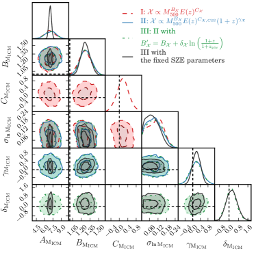
Figure 8: Similar to Figure 5 but containing constraints for the case of $M_{\mathrm{ICM}}-M_{500}-z$ scaling relations.

5.2.1 Parameter constraints

We present the best-fit parameters of the $M_{\mathrm{ICM}}-M_{500}-z$ relations using the scaling relation forms I, II, and III (equations 10, 11 and 12) in Table 4, and the marginalized posteriors of the single and joint parameter constraints are presented in Figure 8. We do not present core-excised values for the ICM mass, because the central core region contains only a negligible portion of the ICM. The best-fit $M_{\mathrm{ICM}}-M_{500}-z$ scaling relation using Form II is

$$M_{\mathrm{ICM}} = 7.37^{+0.76}_{-1.35}\times 10^{13}M_{\odot}\left(\frac{M_{500}}{M_{\mathrm{piv}}}\right)^{1.26^{+0.12}_{-0.09}}\times$$ (21)

$$\left(\frac{1+z}{1+z_{\mathrm{piv}}}\right)^{0.18^{+0.30}_{-0.31}}\,,$$

with intrinsic scatter of $0.10^{+0.04}_{-0.07}$. As before, the mass and redshift pivots are $M_{\mathrm{piv}}=6.35\times 10^{14}M_{\odot}$ and $z_{\mathrm{piv}}=0.45$.

We find that the mass trend parameter is $B_{M_{\mathrm{ICM}}}=1.26^{+0.12}_{-0.09}$, which is steeper than the self-similar scaling at the $\approx 2.9\sigma$ level. Although the uncertainties are large, there are no significant redshift trends observed. The data provide no evidence for a redshift-dependent mass slope, given that $\delta_{M_{\mathrm{ICM}}}$ of $0.16^{+0.47}_{-0.44}$. The normalization $A_{M_{\mathrm{ICM}}}$ of $7.37^{+0.76}_{-1.35}\times 10^{13}M_{\odot}$ suggests an ICM mass fraction of $\approx(16.0\pm 2)\%$ at the pivot mass and redshift. A consistent picture is suggested by all three functional forms. Furthermore, fixing the SZE parameters $r_{\zeta}$ does not shift the best-fit parameters, but reduces the uncertainty of the normalization by a factor of four and the uncertainties on the mass and redshift trends by a factor of two.

5.2.2 Comparison to previous results

We show the redshift and mass trends of $M_{\mathrm{ICM}}$ in the second row from the top of Figs. 3 and 4, respectively. As for the case of the other X-ray observables shown in this plot, we scale the measurements to the pivot redshift $z_{\mathrm{piv}}=0.45$ or pivot mass $M_{\mathrm{piv}}=6.35\times 10^{14}M_{\odot}$ using the best-fit redshift and mass trends from the Form II relation (see Table 4).

Our measured mass trends are consistent with that found by Zhang et al. (2012, $B_{M_{\mathrm{ICM}}}=1.38\pm 0.36$), where a sample of 19 clusters ($z<0.1$ and $2\times 10^{14}M_{\odot}\lesssim M_{500}\lesssim 2\times 10^{15}M_{\odot}$) selected by their X-ray fluxes was studied, and also in the study of the 100 brightest galaxy clusters and groups at redshift range of 0.05–1.1 and and mass range of $10^{13}-10^{15}M_{\odot}$) selected from the XXL survey ($B_{M_{\mathrm{ICM}}}=1.21^{+0.11}_{-0.10}$; Eckert et al., 2016). The mass trends derived from low-redshift clusters (Arnaud et al., 2007; Pratt et al., 2009, $1.24\pm 0.06$ and $1.21\pm 0.03$, respectively) using hydrostatic masses are also consistent with our measurement. Our derived mass trends are in good agreement with those derived based on the SPT clusters observed with Chandra (Chiu et al., 2016b, 2018, $B_{M_{\mathrm{ICM}}}=1.33\pm 0.07$). The agreement between our results and previous Chandra-based works of SPT-selected clusters indicates that $M_{\mathrm{ICM}}-M_{500}-z$ relation is relatively insensitive to the instrumental systematics.

In two other works, mass trends more consistent with self-similar behavior have been found. Our results are in tension with the Mahdavi et al. (2013, $B_{M_{\mathrm{ICM}}}=1.04\pm 0.10$) weak lensing analysis at $\approx 1.6\sigma$ and with Mantz et al. (2016, $B_{M_{\mathrm{ICM}}}=1.004\pm 0.015$) analysis of massive, RASS selected clusters at $\approx 2.9\sigma$. The tension with the Mantz et al. (2016) results is particularly strong, but in general we find that our results are in excellent agreement with those from past studies carried out either with weak lensing or hydrostatic masses. Most previous studies have been carried out over a narrower range of lower redshifts. And indeed, as already noted, our data provide no evidence for a redshift dependent mass slope.

Similarly, In Figure 7 we also compare our results with simulated clusters (Barnes et al., 2017), together with Pratt et al. (2009), Vikhlinin et al. (2009a) and Mantz et al. (2016). Note that in addition to shifting the hydrostatic mass based halo masses as described in the previous section, here we also scale up the $M_{\mathrm{ICM}}$ measurements in the literature by $3.8\%$ because $M_{\mathrm{ICM}}$ is increasing linearly with cluster radius (i.e., $M_{\mathrm{ICM}}\propto R_{500}\propto{M_{500}}^{\frac{1}{3}}$). In the case of the ICM mass, our results show good agreement with the simulations and with the previous results, although with a steeper mass trend in comparison to Mantz et al. (2016) (see the discussion above).

It is worth noting that the intrinsic scatter $\sigma_{\ln M_{\mathrm{ICM}}}$ in $M_{\mathrm{ICM}}$ at fixed halo mass is at the $\approx 10\%$ level, indicating that the ICM mass is among the highest quality cluster mass proxies available.

5.3 $Y_{\mathrm{X}}-M_{500}-z$ Relation

The X-ray estimated integrated pressure $Y_{\mathrm{X}}$ is of interest because of relatively low intrinsic scatter, its connection to the SZE observable and its relative insensitivity to the influence of feedback from AGN and star formation (Kravtsov et al., 2006; Nagai et al., 2007; Bonamente et al., 2008; Vikhlinin et al., 2009a; Andersson et al., 2011; Benson et al., 2013). The self-similar expectation of the $Y_{\mathrm{X}}$ to mass scaling relations is;

$$Y_{\mathrm{X}}\propto M_{500}^{5/3}\ E(z)^{2/3},$$ (22)

which results from $Y_{\mathrm{X}}$ being the product of $M_{\mathrm{ICM}}$ and ${T_{\mathrm{X}}}$ together with the dependence of the $T_{\mathrm{X}}-M_{500}-z$ relation on the evolution of the critical density.

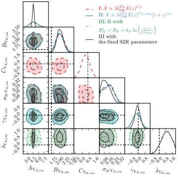
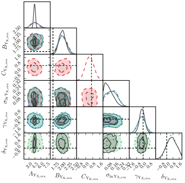
Figure 9: Similar to Figure 5 but containing constraints for the cases of the core-excised $Y_{\mathrm{X,cin}}-M_{500}-z$  (the upper panel) and core-included $Y_{\mathrm{X,cex}}-M_{500}-z$ (the lower panel) scaling relations.

5.3.1 Parameter constraints

Similar to previous sections, we present the $Y_{\mathrm{X}}-M_{500}-z$ relation derived using both the core-included $Y_{\mathrm{X,cin}}$ and -excised $Y_{\mathrm{X,cex}}$ observables for the scaling relations forms I, II, and III (equations 10, 11 and 12, respectively). The best-fit parameters and uncertainties of the scaling relations are listed in Table 4 for both $Y_{\mathrm{X}}$ observables, and the marginalized posteriors of the single and joint parameters are presented in Figure 9.

The best-fit $Y_{\mathrm{X}}-M_{500}-z$ scaling relation using functional form II in the core-included case is

$$Y_{\mathrm{X,cin}} = 4.6^{+1.1}_{-1.1}\times 10^{14}~{}M_{\odot}\mathrm{keV}\left(\frac{M_{500}}{M_{\mathrm{piv}}}\right)^{1.99^{+0.17}_{-0.15}}$$ (23)

$$\left(\frac{E(z)}{E(z_{\mathrm{piv}})}\right)^{\frac{2}{3}}\left(\frac{1+z}{1+z_{\mathrm{piv}}}\right)^{-0.21^{+0.50}_{-0.45}},$$

with intrinsic scatter of $0.16^{+0.05}_{-0.12}$. For the core-excised observable $Y_{\mathrm{X,cex}}$ the best-fit relation is

$$Y_{\mathrm{X,cex}} = 4.50^{+1.00}_{-1.10}\times 10^{14}~{}M_{\odot}\mathrm{keV}\left(\frac{M_{500}}{M_{\mathrm{piv}}}\right)^{2.02^{+0.16}_{-0.17}}\times$$ (24)

$$\left(\frac{E(z)}{E(z_{\mathrm{piv}})}\right)^{\frac{2}{3}}\left(\frac{1+z}{1+z_{\mathrm{piv}}}\right)^{-0.17^{+0.47}_{-0.50}}\,,$$

with intrinsic scatter $0.11^{+0.07}_{-0.08}$. As for all other cases, the mass and redshift pivots are $M_{\mathrm{piv}}=6.35\times 10^{14}M_{\odot}$ and $z_{\mathrm{piv}}=0.45$.

For $Y_{\mathrm{X}}-M_{500}-z$ relations, we observe the mass trend $B_{Y_{\mathrm{X}}}$ that is in tension with the self-similar prediction at the $\approx 2\sigma$ level for the core-included and -excised X-ray observables. On the other hand, the redshift trends for all three functional forms are consistent with self-similarity within the quoted $1\sigma$ uncertainty. There is no evidence for a redshift-dependent mass trend. Fixing the SZE parameters $r_{\zeta}$ leads to no major parameter shifts, but does reduce the parameter uncertainties on the normalization by a factor of about four and, interestingly, leads to a reduction in the estimate of the intrinsic scatter. With intrinsic scatter at the $\approx 10\%$ level as with the $M_{\mathrm{ICM}}$, the $Y_{\mathrm{X}}$ observable with or without core excision offers an outstanding single cluster mass proxy.

5.3.2 Comparison to previous results

We show the redshift and mass trends of $Y_{\mathrm{X}}$ in the third row from the top of Figs. 3 and 4, respectively. As for the case of the other X-ray observables shown in this plot, we scale the measurements to the pivot redshift $z_{\mathrm{piv}}=0.45$ or pivot mass $M_{\mathrm{piv}}=6.35\times 10^{14}M_{\odot}$ using the best-fit redshift and mass trends from the Form II relation (see Table 4).

Given that we are adopting halo masses from the $\zeta-M_{500}-z$ scaling relation calibrated in the analysis of de Haan et al. (2016), we note that the slope of the $Y_{\mathrm{X}}-M_{500}-z$ relation was found in that work to favor a scaling steeper than its self similar predicted value (i.e., $\approx$2 vs 1.67). In this work, we measure X-ray observables (${T_{\mathrm{X}}}$, $M_{\mathrm{ICM}}$, $Y_{\mathrm{X}}$, and $L_{\mathrm{X}}$) for the SPT-SZ cluster sample using a different set of observations from the XMM-Newton satellite. While these data are independent of the data used in de Haan et al. (2016), one would nevertheless expect that given the results of that earlier analysis using Chandra data, that we should see a $Y_{\mathrm{X}}-M_{500}-z$ relation that is steeper than self-similar, as indeed we do.

In comparison to other previously published results, the constraints on the mass trend of the full sample is steeper than the reported value in Arnaud et al. (2007, $B_{Y_{\mathrm{X}}}=1.83\pm 0.09$), a difference of $\approx 1\sigma$. Other studies employing X-ray hydrostatic masses also resulted in shallower slopes (Vikhlinin et al., 2009a; Lovisari et al., 2015, $B_{Y_{\mathrm{X}}}=1.75\pm 0.09$ and $B_{Y_{\mathrm{X}}}=1.67\pm 0.08$, respectively), which also show weak tension with our results at 1.4 and 1.8$\sigma$ significance, respectively. The weak lensing based study of Mahdavi et al. (2013) also found a weaker mass trend of $B_{Y_{\mathrm{X}}}=1.79\pm 0.22$ that is nonetheless statistically consistent with our results. The tension between our result and the Mantz et al. (2016) analysis ($B_{Y_{\mathrm{X}}}=1.61\pm 0.04$) is at the 2.3$\sigma$ level.

In Figure 7 we also compare our core-excised $Y_{\mathrm{X,cex}}$ with simulated clusters (Barnes et al., 2017) and the observations from Pratt et al. (2009) and Vikhlinin et al. (2009a). Similar to the case of ICM mass, we also scale up the $Y_{\mathrm{X,cex}}$ by $3.8\%$ because of $Y_{\mathrm{X,cex}}\equiv{T_{\mathrm{X,cex}}}M_{\mathrm{ICM}}$. Our results are broadly consistent with both the simulated and observed clusters but with a preference for a slope that is steeper than the self-similar prediction.

As with the $T_{\mathrm{X}}-M_{500}-z$ relations presented previously, our measured $Y_{\mathrm{X}}$ mass trends are steeper and exhibit greater tension with self-similar behavior than previous works. This can be understood as the combination of the ${T_{\mathrm{X}}}$ and $M_{\mathrm{ICM}}$ mass trends—each steeper than self-similar—presented in the last two sections. However, while the $M_{\mathrm{ICM}}-M_{500}-z$ relation mass trend we measure is in good agreement with previous analyses, it is our $T_{\mathrm{X}}-M_{500}-z$ relation that appears steeper. Whether this is due to our unique SZE-selection, leading to an approximately mass-limited sample over a very large redshift range, or due to systematic differences in our mass estimates that include Eddington and Malmquist bias corrections that are typically not considered in earlier works, this must be clarified with a larger sample of clusters and with the ongoing improvements in mass calibration of our own sample.

5.4 $L_{\mathrm{X}}-M_{500}-z$ Relation

We extract the X-ray luminosity obtained from the core-included aperture of $<R_{500}$ in the 0.5–2 keV (i.e., the soft-band luminosity $L_{\mathrm{X}}$) and the 0.01:100 keV band (i.e., the bolometric luminosity $L_{\mathrm{X,bol}}$) to study the $L_{\mathrm{X}}-M_{500}-z$ scaling relations. In previous studies, the $L_{\mathrm{X}}-M_{500}-z$ scaling relations have tended to exhibit larger scatter if cluster cores are included in the analysis (Pratt et al., 2009) due to the complex cool-core phenomenon that impacts the central regions of clusters. Indeed, it was argued long ago that the primary driver of the $L_{\mathrm{X}}-{T_{\mathrm{X}}}$ relation scatter was this cool core phenomenon (Fabian et al., 1994), and with the availability of cluster samples extending to high redshift it was shown to be true out to $z\approx 0.8$ (O’Hara et al., 2006). Therefore, we also additionally extract the X-ray luminosities obtained from the core-excised aperture of $(0.15-1)R_{500}$ in both soft and bolometric bands. As a result, we derive four $L_{\mathrm{X}}-M_{500}-z$ scaling relations—(1) core-included and soft-band luminosity to mass $L_{\mathrm{X,cin}}$–$M_{500}$, (2) core-included and bolometric luminosity to mass $L_{\mathrm{X,cin,bol}}$–$M_{500}$, (3) core-excised and soft-band luminosity to mass $L_{\mathrm{X,cex}}$–$M_{500}$, and (4) core-excised and bolometric luminosity to mass $L_{\mathrm{X,cex,bol}}$–$M_{500}$ scaling relations. The self-similar expectation of the $L_{\mathrm{X}}-M_{500}-z$ scaling relation is

$$L_{\mathrm{X}} \propto M_{500}\ E(z)^{2}\,.$$

$$L_{\mathrm{X,bol}} \propto M_{500}^{4/3}\ E(z)^{7/3}\,.$$

for the the soft-band and bolometric luminosities, respectively, where for the soft-band we have assumed that the emissivity is temperature independent (see discussion in Mohr et al., 1999).

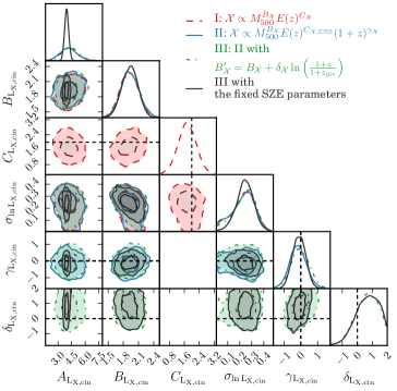
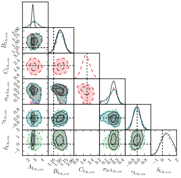
Figure 10: Similar to Figure 5 but containing constraints for the cases of the 0.5:2.0 keV core-included luminosity $L_{\mathrm{X,cin}}-M_{500}-z$ (the upper panel) and core-excised luminosity $L_{\mathrm{X,cex}}-M_{500}-z$ (the lower panel) scaling relations.

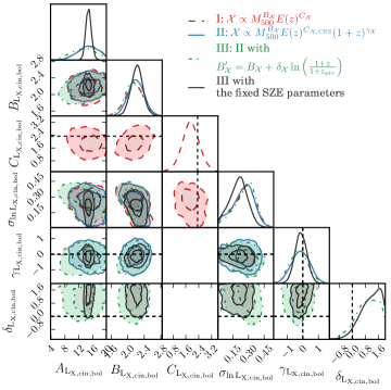
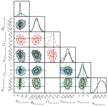
Figure 11: Similar to Figure 5 but containing constraints for the cases of the core-included bolometric luminosity $L_{\mathrm{X,cin}}-M_{500}-z$ (the upper panel) and core-excised bolometric luminosity $L_{\mathrm{X,cex}}-M_{500}-z$ (the lower panel) scaling relations.

5.4.1 Parameter constraints

The resulting best-fit scaling relation parameters and uncertainties are listed in Table 4, and the marginalized posteriors of the single and joint parameters constraints for the core-included and -excised observables appear in Figure 10 (0.5–2.0 keV) and Figure 11 (bolometric).

For the core-included, soft-band 0.5–2.0 keV X-ray luminosity $L_{\mathrm{X,cin}}$, the best-fit relation is

$$L_{\mathrm{X,cin}} = 4.12^{+0.91}_{-0.94}\times 10^{44}\mathrm{erg/s}\left(\frac{M_{500}}{M_{\mathrm{piv}}}\right)^{1.89^{+0.23}_{-0.13}}$$ (26)

$$\left(\frac{E(z)}{E(z_{\mathrm{piv}})}\right)^{2}\left(\frac{1+z}{1+z_{\mathrm{piv}}}\right)^{-0.20^{+0.51}_{-0.49}}\,,$$

with intrinsic scatter of $0.27^{+0.08}_{-0.12}$. For the $L_{\mathrm{X,cex}}-M_{500}-z$ relation, the best-fit is

$$L_{\mathrm{X,cex}} = 2.84^{+0.53}_{-0.50}\times 10^{44}\mathrm{erg/s}\left(\frac{M_{500}}{M_{\mathrm{piv}}}\right)^{1.60^{+0.16}_{-0.15}}$$ (27)

$$\left(\frac{E(z)}{E(z_{\mathrm{piv}})}\right)^{2}\left(\frac{1+z}{1+z_{\mathrm{piv}}}\right)^{-0.10^{+0.47}_{-0.42}},$$

with intrinsic scatter of $0.27^{+0.07}_{-0.11}$. As before, the mass and redshift pivots are $M_{\mathrm{piv}}=6.35\times 10^{14}M_{\odot}$ and $z_{\mathrm{piv}}=0.45$.

The soft-band, core-excised $L_{\mathrm{X}}-M_{500}-z$ relation shows a mass trend that is $\approx 4\sigma$ higher than the self-similar trend ($B_{L_{\mathrm{X}}}=1$), while the core-included relation is steeper and exhibits a tension of $\approx 6.8\sigma$ with the self-similar behavior. The redshift trends for both core-included and -excised luminosities are consistent with the self-similar trend of $C_{L_{\mathrm{X}}}=2$. There is no evidence for a redshift-dependent mass slope in either soft-band $L_{\mathrm{X}}$ measurement. Fixing the SZE parameters $r_{\zeta}$ (the black curves in Figure 10) does not change the overall picture except that the uncertainties of the normalization are reduced by about a factor of four.

The characteristic luminosities at the pivot mass and redshift for core-included clusters are a factor of $\approx 45\%$ higher than the core-excised luminosities, a difference of $\approx 1\sigma$. Interestingly, the scatter of the two relations is similar at $\approx 27\%$.

Similarly, for the bolometric luminosities the best-fit $L_{\mathrm{X,cin,bol}}-M_{500}-z$ and $L_{\mathrm{X,cex,bol}}-M_{500}-z$ relations are

$$L_{\mathrm{X,cin}} = 14.8^{+3.5}_{-2.7}\times 10^{44}\mathrm{erg/s}\left(\frac{M_{500}}{M_{\mathrm{piv}}}\right)^{2.19^{+0.21}_{-0.17}}$$ (28)

$$\left(\frac{E(z)}{E(z_{\mathrm{piv}})}\right)^{\frac{7}{3}}\left(\frac{1+z}{1+z_{\mathrm{piv}}}\right)^{-0.14^{+0.62}_{-0.57}}\,,$$

and

$$L_{\mathrm{X,cex}} = 10.7^{+2.3}_{-2.3}\times 10^{44}\mathrm{erg/s}\left(\frac{M_{500}}{M_{\mathrm{piv}}}\right)^{1.88^{+0.19}_{-0.17}}$$ (29)

$$\left(\frac{E(z)}{E(z_{\mathrm{piv}})}\right)^{\frac{7}{3}}\left(\frac{1+z}{1+z_{\mathrm{piv}}}\right)^{-0.26^{+0.53}_{-0.43}},$$

with intrinsic scatter of $0.29^{+0.08}_{-0.13}$ and $0.27^{+0.07}_{-0.13}$, respectively. The same pivot mass and redshift as before are used.

As expected, the bolometric luminosity relations have steeper mass trends than those of the soft band luminosities. Similar to the soft band, the bolometric luminosity to mass scaling relations have mass trends that are steeper than self-similar ($B_{L_{\mathrm{X}}}={4\over 3}$) with a significance of $\approx 3.2\sigma$ and $\approx 5.1\sigma$ for the core-excised and core-included luminosities, respectively. The redshift trends of the scaling relations are all consistent with the self-similar trend $C_{L_{\mathrm{X}}}={7\over 3}$, and there is a preference for a redshift dependent mass trend in the core-included luminosity scaling relation. Fixing the SZE parameters $r_{\zeta}$ does not result in significant differences except by decreasing the uncertainties of the normalization by a factor of three to five, and it also slightly reduces the scatter in the core-included relation. Both relations exhibit intrinsic scatter at around the $27\%$ level, which is comparable to that in the soft band.

5.4.2 Comparison to previous results

We show the redshift and mass trends of $L_{\mathrm{X}}$ in the two bottom rows in Figures  3 and 4, respectively. As for the case of the other X-ray observables shown in this plot, we scale the measurements to the pivot redshift $z_{\mathrm{piv}}=0.45$ or pivot mass $M_{\mathrm{piv}}=6.35\times 10^{14}M_{\odot}$ using the best-fit redshift and mass trends from the Form II relation (see Table 4).

Our core-excised bolometric luminosities are consistent with the bolometric luminosities reported from XMM-Newton observations of the low-z REXCESS clusters (Pratt et al., 2009, with a slope of $1.77\pm 0.05$). Additionally, our core-excised soft-band luminosities from Chandra and XMM-Newton observations of the 15 SPT selected clusters (Andersson et al., 2011, with a slope of $1.45\pm 0.29$), Chandra observations of massive clusters Vikhlinin et al. (2009b, with a slope of $1.61\pm 0.14$), Chandra observations of 115 clusters (Maughan, 2007, with a slope of $1.63\pm 0.08$), and the XMM-Newton observations of HIFLUGCS sample (Lovisari et al., 2015, with a slope of $1.61\pm 0.19$) at $z<0.05$. We note that all these results in the literature depart from the self-similar expectation. However, the slope of the mass trend of the core-excised soft-band luminosity ($B_{L_{\mathrm{X}}}\approx 1.60\pm 0.15$) is steeper than the value reported in Mantz et al. (2016, $B_{L_{\mathrm{X}}}=1.02\pm 0.09$) at the $3.4\sigma$ level. Our slope is consistent with the low-redshift ($z<0.2$) HIFLUGCS Cosmology (HICOSMO) sample ($B_{L_{\mathrm{X}}}=1.35\pm 0.07$; Schellenberger et al., 2015) at $\approx 1.5\sigma$ level. Overall, in terms of mass trends our study demonstrates a much steeper than self-similar mass trend in agreement with most previously published analyses.

Our constraints on the redshift trend of the core-excised, soft-band $L_{\mathrm{X}}-M_{500}-z$ is $L_{L_{\mathrm{X}}}\propto E(z)^{1.72^{+0.53}_{-0.46}}$, which is in good agreement with that found by Mantz et al. (2016, $C_{L_{\mathrm{X}}}=1.82\pm 0.35$). Vikhlinin et al. (2009b) reports a redshift trend of $C_{L_{\mathrm{X}}}=1.85\pm 0.40$, which is also consistent with our results. In addition, our soft band measurements follow a similar trend with that seen in the C-Eagle cosmological hydrodynamical simulations of clusters (Barnes et al., 2017).

In Figure  7, we over-plot our results of core-excised soft-band luminosity $L_{\mathrm{X,cex}}$ with the ones from simulated clusters (Barnes et al., 2017) and other observational studies (Pratt et al., 2009; Vikhlinin et al., 2009a; Mantz et al., 2016). Although our SPT clusters are sampling the relatively high-mass end, our results show no significant tension in the mass trend with previous work extending to the low mass regime. With the exception of the analysis of Mantz et al. (2016), the $L_{\mathrm{X,cex}}$ from both simulated and observed clusters all show steeper mass trends with respect to the self-similar prediction (the grey dashed line). We note also that the scatter in the simulated C-Eagle clusters is 0.30, which is larger than, but statistically consistent with, our measurement of $\sigma_{\ln L_{\mathrm{X}}}=0.27^{+0.07}_{-0.11}$. This is also true for the values of 0.17 and 0.25 found in the REXCESS (Pratt et al., 2009) and HIFLUGCS samples (Lovisari et al., 2015). An interesting element of our result is that the scatter is similar in both the core-included and -excised luminosity measurements.

Table 5: This table holds the best-fit scaling relation parameters when priors on the SZE $\zeta-M_{500}-z$ relation parameters are taken from de Haan et al. (2016, Table 3, results column 2). The Table layout is the same as in Table 4.

Scaling Relation	$A_{\mathcal{X}}$	$B_{\mathcal{X}}$	$C_{\mathcal{X}}$	$\sigma_{\ln\mathcal{X}}$	$\gamma_{\mathcal{X}}$	$\delta_{\mathcal{X}}$
$T_{\mathrm{X,cin}}-M_{500}-z$ Relation		$B_{\mathrm{\mathcal{X},SS}}={2\over 3}$	$C_{\mathrm{\mathcal{X},SS}}={2\over 3}$
I: $\mathcal{X}(M,z)\propto M_{500}^{B_{\mathcal{X}}}E(z)^{C_{\mathcal{X}}}$	$6.50\pm 0.66$	$0.78^{+0.10}_{-0.09}$	$0.44^{+0.27}_{-0.26}$	$0.18^{+0.04}_{-0.05}$	–	–
II: $\mathcal{X}(M,z)\propto M_{500}^{B_{\mathcal{X}}}E(z)^{2\over 3}(1+z)^{\gamma_{\mathcal{X}}}$	$6.51^{+0.58}_{-0.70}$	$0.81^{+0.09}_{-0.10}$	$2\over 3$	$0.18^{+0.04}_{-0.04}$	$-0.21^{+0.24}_{-0.22}$	–
III: as II with $B^{\prime}_{\mathcal{X}}=B_{\mathcal{X}}+\delta_{\mathcal{X}}\ln\left(\frac{1+z}{1+z_{\mathrm{piv}}}\right)$	$6.42^{+0.67}_{-0.65}$	$0.77^{+0.10}_{-0.09}$	$2\over 3$	$0.17^{+0.05}_{-0.03}$	$-0.14^{+0.33}_{-0.26}$	$0.60^{+0.57}_{-0.47}$
III with fixed SZE params	$6.44^{+0.24}_{-0.23}$	$0.79^{+0.08}_{-0.09}$	$2\over 3$	$0.17^{+0.04}_{-0.03}$	$-0.05^{+0.25}_{-0.27}$	$0.81^{+0.49}_{-0.53}$
$T_{\mathrm{X,cex}}-M_{500}-z$ Relation		$B_{\mathrm{\mathcal{X},SS}}={2\over 3}$	$C_{\mathrm{\mathcal{X},SS}}={2\over 3}$
I: $\mathcal{X}(M,z)\propto M_{500}^{B_{\mathcal{X}}}E(z)^{C_{\mathcal{X}}}$	$6.26^{+0.57}_{-0.68}$	$0.80^{+0.10}_{-0.08}$	$0.43^{+0.23}_{-0.22}$	$0.13^{+0.04}_{-0.06}$	–	–
II: $\mathcal{X}(M,z)\propto M_{500}^{B_{\mathcal{X}}}E(z)^{2\over 3}(1+z)^{\gamma_{\mathcal{X}}}$	$6.25^{+0.49}_{-0.75}$	$0.81^{+0.08}_{-0.09}$	$2\over 3$	$0.14^{+0.04}_{-0.06}$	$-0.20^{+0.21}_{-0.22}$	–
III: as II with $B^{\prime}_{\mathcal{X}}=B_{\mathcal{X}}+\delta_{\mathcal{X}}\ln\left(\frac{1+z}{1+z_{\mathrm{piv}}}\right)$	$6.18^{+0.63}_{-0.62}$	$0.81^{+0.10}_{-0.10}$	$2\over 3$	$0.14^{+0.04}_{-0.05}$	$-0.17^{+0.28}_{-0.23}$	$0.35^{+0.41}_{-0.45}$
III with fixed SZE params	$6.14^{+0.22}_{-0.17}$	$0.81^{+0.08}_{-0.08}$	$2\over 3$	$0.13^{+0.04}_{-0.04}$	$-0.13\pm 0.23$	$0.45^{+0.41}_{-0.48}$
$M_{\mathrm{ICM}}-M_{500}-z$ Relation		$B_{\mathrm{\mathcal{X},SS}}=1$	$C_{\mathrm{\mathcal{X},SS}}=0$
I: $\mathcal{X}(M,z)\propto M_{500}^{B_{\mathcal{X}}}E(z)^{C_{\mathcal{X}}}$	$6.60^{+1.1}_{-1.0}$	$1.27^{+0.08}_{-0.11}$	$0.43^{+0.24}_{-0.23}$	$0.11^{+0.04}_{-0.08}$	–	–
II: $\mathcal{X}(M,z)\propto M_{500}^{B_{\mathcal{X}}}E(z)^{0}(1+z)^{\gamma_{\mathcal{X}}}$	$7.14^{+1.00}_{-1.01}$	$1.26^{+0.09}_{-0.10}$	$0$	$0.11^{+0.04}_{-0.08}$	$0.39^{+0.25}_{-0.24}$	–
III: as II with $B^{\prime}_{\mathcal{X}}=B_{\mathcal{X}}+\delta_{\mathcal{X}}\ln\left(\frac{1+z}{1+z_{\mathrm{piv}}}\right)$	$6.89^{+1.15}_{-0.91}$	$1.27^{+0.10}_{-0.10}$	$0$	$0.11^{+0.03}_{-0.08}$	$0.40^{+0.23}_{-0.24}$	$0.19^{+0.40}_{-0.54}$
III with fixed SZE params	$6.93^{+0.28}_{-0.19}$	$1.27^{+0.08}_{-0.08}$	$0$	$0.08^{+0.04}_{-0.06}$	$0.41^{+0.21}_{-0.22}$	$0.11^{+0.44}_{-0.47}$
$Y_{\mathrm{X,cin}}-M_{500}-z$ Relation		$B_{\mathrm{\mathcal{X},SS}}={5\over 3}$	$C_{\mathrm{\mathcal{X},SS}}={2\over 3}$
I: $\mathcal{X}(M,z)\propto M_{500}^{B_{\mathcal{X}}}E(z)^{C_{\mathcal{X}}}$	$4.5^{+1.0}_{-1.1}$	$2.00^{+0.16}_{-0.14}$	$0.80^{+0.42}_{-0.35}$	$0.15^{+0.08}_{-0.09}$	–	–
II: $\mathcal{X}(M,z)\propto M_{500}^{B_{\mathcal{X}}}E(z)^{2\over 3}(1+z)^{\gamma_{\mathcal{X}}}$	$4.7^{+1.1}_{-1.0}$	$2.01^{+0.16}_{-0.14}$	$2\over 3$	$0.15^{+0.07}_{-0.11}$	$0.15^{+0.39}_{-0.34}$	–
III: as II with $B^{\prime}_{\mathcal{X}}=B_{\mathcal{X}}+\delta_{\mathcal{X}}\ln\left(\frac{1+z}{1+z_{\mathrm{piv}}}\right)$	$4.9\pm 1.1$	$2.03^{+0.13}_{-0.15}$	$2\over 3$	$0.17^{+0.06}_{-0.10}$	$0.32^{+0.39}_{-0.41}$	$1.16^{+0.44}_{-0.77}$
III with fixed SZE params	$4.59^{+0.22}_{-0.27}$	$1.97\pm 0.11$	$2\over 3$	$0.07^{+0.07}_{-0.06}$	$0.23^{+0.35}_{-0.33}$	$0.73^{+0.77}_{-0.55}$
$Y_{\mathrm{X,cex}}-M_{500}-z$ Relation		$B_{\mathrm{\mathcal{X},SS}}={5\over 3}$	$C_{\mathrm{\mathcal{X},SS}}={2\over 3}$
I: $\mathcal{X}(M,z)\propto M_{500}^{B_{\mathcal{X}}}E(z)^{C_{\mathcal{X}}}$	$4.25^{+0.96}_{-1.02}$	$1.99^{+0.14}_{-0.16}$	$0.77^{+0.37}_{-0.42}$	$0.13^{+0.05}_{-0.10}$	–	–
II: $\mathcal{X}(M,z)\propto M_{500}^{B_{\mathcal{X}}}E(z)^{2\over 3}(1+z)^{\gamma_{\mathcal{X}}}$	$4.35^{+0.90}_{-1.10}$	$2.00^{+0.16}_{-0.15}$	$2\over 3$	$0.05^{+0.12}_{-0.03}$	$0.09^{+0.44}_{-0.29}$	–
III: as II with $B^{\prime}_{\mathcal{X}}=B_{\mathcal{X}}+\delta_{\mathcal{X}}\ln\left(\frac{1+z}{1+z_{\mathrm{piv}}}\right)$	$4.70^{+1.1}_{-1.2}$	$1.99^{+0.18}_{-0.14}$	$2\over 3$	$0.13^{+0.05}_{-0.10}$	$0.35^{+0.38}_{-0.41}$	$0.47^{+0.63}_{-0.65}$
III with fixed SZE params	$4.31^{+0.30}_{-0.18}$	$1.98\pm 0.12$	$2\over 3$	$0.04^{+0.09}_{-0.03}$	$0.27^{+0.33}_{-0.35}$	$0.72^{+0.57}_{-0.69}$
$L_{\mathrm{X,cin}}-M_{500}-z$ Relation		$B_{\mathrm{\mathcal{X},SS}}={1}$	$C_{\mathrm{\mathcal{X},SS}}={2}$
I: $\mathcal{X}(M,z)\propto M_{500}^{B_{\mathcal{X}}}E(z)^{C_{\mathcal{X}}}$	$4.13^{+0.87}_{-0.98}$	$1.93^{+0.15}_{-0.18}$	$2.01^{+0.44}_{-0.37}$	$0.28^{+0.07}_{-0.12}$	–	–
II: $\mathcal{X}(M,z)\propto M_{500}^{B_{\mathcal{X}}}E(z)^{2}(1+z)^{\gamma_{\mathcal{X}}}$	$4.15^{+1.10}_{-0.81}$	$1.91^{+0.18}_{-0.15}$	$2$	$0.25^{+0.08}_{-0.13}$	$0.20^{+0.41}_{-0.43}$	–
III: as II with $B^{\prime}_{\mathcal{X}}=B_{\mathcal{X}}+\delta_{\mathcal{X}}\ln\left(\frac{1+z}{1+z_{\mathrm{piv}}}\right)$	$4.33^{+1.11}_{-0.89}$	$1.85^{+0.21}_{-0.16}$	$2$	$0.28^{+0.08}_{-0.11}$	$0.21^{+0.53}_{-0.44}$	$0.82^{+0.61}_{-0.94}$
III with fixed SZE params	$3.86^{+0.22}_{-0.20}$	$1.94\pm 0.15$	$2$	$0.23^{+0.08}_{-0.07}$	$0.33^{+0.42}_{-0.37}$	$0.79^{+0.83}_{-0.65}$
$L_{\mathrm{X,cex}}-M_{500}-z$ Relation		$B_{\mathrm{\mathcal{X},SS}}={1}$	$C_{\mathrm{\mathcal{X},SS}}={2}$
I: $\mathcal{X}(M,z)\propto M_{500}^{B_{\mathcal{X}}}E(z)^{C_{\mathcal{X}}}$	$2.83^{+0.53}_{-0.52}$	$1.57^{+0.17}_{-0.14}$	$2.17^{+0.34}_{-0.43}$	$0.26^{+0.07}_{-0.09}$	–	–
II: $\mathcal{X}(M,z)\propto M_{500}^{B_{\mathcal{X}}}E(z)^{2}(1+z)^{\gamma_{\mathcal{X}}}$	$2.82^{+0.61}_{-0.49}$	$1.63^{+0.13}_{-0.16}$	$2$	$0.26^{+0.08}_{-0.09}$	$0.20^{+0.41}_{-0.34}$	–
III: as II with $B^{\prime}_{\mathcal{X}}=B_{\mathcal{X}}+\delta_{\mathcal{X}}\ln\left(\frac{1+z}{1+z_{\mathrm{piv}}}\right)$	$2.77^{+0.55}_{-0.51}$	$1.57^{+0.18}_{-0.16}$	$2$	$0.28^{+0.07}_{-0.07}$	$0.24^{+0.51}_{-0.32}$	$0.47^{+0.93}_{-0.57}$
III with fixed SZE params	$2.67^{+0.16}_{-0.15}$	$1.58\pm 0.15$	$2$	$0.26^{+0.06}_{-0.05}$	$0.25\pm 0.38$	$0.75^{+0.76}_{-0.74}$
$L_{\mathrm{X,cin,bol}}-M_{500}-z$ Relation		$B_{\mathrm{\mathcal{X},SS}}={4\over 3}$	$C_{\mathrm{\mathcal{X},SS}}={7\over 3}$
I: $\mathcal{X}(M,z)\propto M_{500}^{B_{\mathcal{X}}}E(z)^{C_{\mathcal{X}}}$	$13.8^{+3.6}_{-3.2}$	$2.21^{+0.15}_{-0.20}$	$2.28^{+0.46}_{-0.41}$	$0.29^{+0.09}_{-0.12}$	–	–
II: $\mathcal{X}(M,z)\propto M_{500}^{B_{\mathcal{X}}}E(z)^{7\over 3}(1+z)^{\gamma_{\mathcal{X}}}$	$14.3\pm 3.2$	$2.18\pm 0.19$	$7\over 3$	$0.26^{+0.09}_{-0.13}$	$0.03^{+0.54}_{-0.37}$	–
III: as II with $B^{\prime}_{\mathcal{X}}=B_{\mathcal{X}}+\delta_{\mathcal{X}}\ln\left(\frac{1+z}{1+z_{\mathrm{piv}}}\right)$	$14.8^{+3.3}_{-2.9}$	$2.16^{+0.19}_{-0.16}$	$7\over 3$	$0.28^{+0.09}_{-0.11}$	$0.19^{+0.44}_{-0.50}$	$1.14^{+0.69}_{-0.76}$
III with fixed SZE params	$14.55^{+0.98}_{-0.70}$	$2.23\pm 0.15$	$7\over 3$	$0.19^{+0.08}_{-0.10}$	$0.35^{+0.39}_{-0.42}$	$1.34^{+0.49}_{-0.74}$
$L_{\mathrm{X,cex,bol}}-M_{500}-z$ Relation		$B_{\mathrm{\mathcal{X},SS}}={4\over 3}$	$C_{\mathrm{\mathcal{X},SS}}={7\over 3}$
I: $\mathcal{X}(M,z)\propto M_{500}^{B_{\mathcal{X}}}E(z)^{C_{\mathcal{X}}}$	$10.6^{+2.5}_{-2.2}$	$1.87^{+0.19}_{-0.16}$	$2.31^{+0.45}_{-0.35}$	$0.26^{+0.08}_{-0.13}$	–	–
II: $\mathcal{X}(M,z)\propto M_{500}^{B_{\mathcal{X}}}E(z)^{7\over 3}(1+z)^{\gamma_{\mathcal{X}}}$	$10.5^{+2.1}_{-2.5}$	$1.87^{+0.20}_{-0.14}$	$7\over 3$	$0.27^{+0.07}_{-0.14}$	$0.10^{+0.47}_{-0.35}$	–
III: as II with $B^{\prime}_{\mathcal{X}}=B_{\mathcal{X}}+\delta_{\mathcal{X}}\ln\left(\frac{1+z}{1+z_{\mathrm{piv}}}\right)$	$9.9^{+2.2}_{-2.1}$	$1.80^{+0.17}_{-0.22}$	$7\over 3$	$0.30^{+0.07}_{-0.09}$	$0.23^{+0.45}_{-0.49}$	$0.73^{+0.78}_{-0.70}$
III with fixed SZE params	$10.06^{+0.54}_{-0.61}$	$1.86^{+0.15}_{-0.16}$	$7\over 3$	$0.25^{+0.05}_{-0.07}$	$0.36^{+0.32}_{-0.49}$	$0.88^{+0.76}_{-0.57}$

5.5 SZE-based halo masses with external cosmological priors from BAO

Currently, the redshift trend parameter on the SZE $\zeta-M_{500}-z$ relation is the least well constrained, and this leads to additional uncertainty in understanding the X-ray observable mass relations. In de Haan et al. (2016, the second column of Table 3), an analysis within the context of a flat $\Lambda$CDM model was undertaken where additional external cosmological priors from BAO were added. This helped reduce the cosmological parameter space consistent with the SPT cluster sample distribution in $\xi$ and redshift, tightening up $\zeta-M_{500}-z$ parameter uncertainties. In addition, the redshift evolution parameter was shifted upward from $C_{\zeta}=0.55\pm 0.3$ to $C_{\zeta}=0.80\pm 0.15$. The combination of the shift and reduction in uncertainties have motivated us to present the scaling relations derived using the X-ray observables together with these SZE-based halo masses. Table 5 contains the results of these relations. We recommend that those particularly interested in obtaining precise redshift trends in the scaling relations should use these results.

6 Conclusions

We present here measurements of the X-ray observables in a sample of 59 SZE selected galaxy clusters with redshifts $0.20<z<1.5$ that have been observed with XMM-Newton. We use these measurements together with SZE-based halo masses $M_{500}$ to study the scaling relations between X-ray observables, halo mass and redshift. A strength of our work is the ability to directly constrain the redshift and mass trends based on an SZE-selected cluster sample spanning a wide range of redshift. This selection is approximately equivalent to a mass selection, and this sample spans a mass range of $3\times 10^{14}M_{\odot}\leq M_{500}\leq 1.8\times 10^{15}M_{\odot}$. The biasing effects in X-ray selected samples due to the X-ray cool core phenomenon are significantly reduced and perhaps even completely removed. This simplifies the interpretation of the results from our analysis.

We use the XMM-Newton observations to derive X-ray observables ${T_{\mathrm{X}}}$, $M_{\mathrm{ICM}}$, $Y_{\mathrm{X}}$, and rest frame 0.5–2.0 keV and bolometric $L_{\mathrm{X}}$. For all these observables—save for the $M_{\mathrm{ICM}}$—we extract both core-included and core-excised quantities, where we define the core to be the region within 0.15$R_{500}$. The cluster halo masses are derived from the SPT $\zeta-M_{500}-z$ scaling relation and are corrected for selection effects, such as Eddington and Malmquist biases as described in detail in other publications (Bocquet et al., 2015). As discussed in detail in Section 4.3, we adopt priors on the $\zeta-M_{500}-z$ scaling relation from the de Haan et al. (2016) joint cosmology and mass calibration analysis, which have since been validated using weak lensing masses of 32 SPT-SZ clusters (Dietrich et al., 2017) and dynamical masses of 110 SPT-SZ clusters (Capasso et al., 2017). These SZE-based halo masses are characteristically uncertain at the $\approx 25\%$ level (statistical and systematic uncertainties combined in quadrature).

We fit our data to three different power-law models (see equations 10, 11 and 12) and derive the best-fit normalization $A_{\mathcal{X}}$, mass trend $B_{\mathcal{X}}$, $E(z)$ redshift trend $C_{\mathcal{X}}$, departure from self-similar redshift trend $\gamma_{\mathcal{X}}$, log-normal intrinsic scatter in the X-ray observable at fixed halo mass $\sigma_{\ln\mathcal{X}}$, and also a redshift dependence to the mass trend $\delta_{\mathcal{X}}$. While all three scaling relation forms are adequate to fit the data, we recommend that those interested in cosmological studies adopt Form II, because it models the departure from self-similar evolution with redshift using a cosmologically agnostic form $(1+z)^{\gamma_{\mathcal{X}}}$. We marginalize over the uncertainties in the SZE-based halo masses, adjusting the radius $R_{500}$ as appropriate in each iteration in the chain and re-extracting the X-ray observables in a self-consistent manner. Thus, the final parameter uncertainties of the X-ray observable–mass scaling relations include both measurement and systematic halo mass uncertainties (see Table 4).

The halo mass scaling relations for ${T_{\mathrm{X}}}$, $M_{\mathrm{ICM}}$, $Y_{\mathrm{X}}$  and $L_{\mathrm{X}}$  are steeper, but statistically consistent (within $2\sigma$ confidence) with the results from the literature. However, we observe significant departures from the Mantz et al. (2016) soft band core-excised luminosity at $3.4\sigma$ level, ICM mass at $2.9\sigma$ level, and $Y_{\mathrm{X}}$ at $2.3\sigma$ level. The mass trends we find in all our scaling relations are steeper than the self-similar behavior at $\gtrsim 1.6\sigma$ confidence. In the case of $M_{\mathrm{ICM}}$ and $L_{\mathrm{X}}$  the mass trends we measure ($M_{\mathrm{ICM}}\propto M_{500}^{1.26\pm 0.10}$ and $L_{\mathrm{X,cex}}\propto M_{500}^{1.60\pm 0.15}$ in soft band) are consistent with most previously published results that employ X-ray selected samples and a mix of weak lensing and hydrostatic masses. However, for ${T_{\mathrm{X}}}$ and $Y_{\mathrm{X}}$ our mass trends (${T_{\mathrm{X,cex}}}\propto M_{500}^{0.80\pm 0.09}$ and $Y_{\mathrm{X,cex}}\propto M_{500}^{2.0\pm 0.16}$) are steeper than most previous work at $\approx 1.6\sigma$ (see parameter $B_{\mathcal{X}}$ in Tables 4 and 5).

In addition, we probe for a redshift-dependent mass trend (Form III, equation 12) and find that the data currently provide no evidence for such a trend, with the highest significance departure from no evolution being in the core-included $Y_{\mathrm{X}}$ and $L_{\mathrm{X}}$ (see parameter $\delta_{\mathcal{X}}$ in Tables 4 and 5).

We examine the redshift trends in all scaling relations, finding no significant departures from the self-similar behavior that arises simply due to the evolution of the critical density with redshift. There is no tension between our results and those from previous studies, although many previous studies were not in a position to examine redshift trends, given the limitations of their samples and the availability of halo mass measurements (see parameter $\gamma_{\mathcal{X}}$ in Tables 4 and 5).

We report the intrinsic scatter in X-ray observable at fixed halo mass $\sigma_{\ln\mathcal{X}}$ for all scaling relations. These indicate exquisite scatter at the $\approx 10\%$ level for $M_{\mathrm{ICM}}$ and core-excised integrated pressure $Y_{\mathrm{X,cex}}$, somewhat higher scatter of $\approx 13\%$ for core-excised temperature ${T_{\mathrm{X,cex}}}$, and scatter of $\approx 27$ percent for X-ray luminosities $L_{\mathrm{X}}$ (see parameter $\sigma_{\ln\mathcal{X}}$ in Tables 4 and 5). We do not account for correlated scatter among the SZE and X-ray observables, because previous analyses of larger SPT-SZ selected samples have failed to detect these effects (de Haan et al., 2016; Dietrich et al., 2017), and therefore they are too small to have an impact on our results.

In all cases, our baseline results are presented in Table 4, and the mass and redshift trends for each observable are highlighted in Figs. 3 and 4. In addition, we present an alternative set of results in Table 5 that have somewhat better defined redshift trends that come from adopting a calibration of the SZE $\zeta-M_{500}-z$ relation that includes external cosmological priors from BAO (see discussion in Section 5.5).

One of the reasons for the steeper mass trends in ${T_{\mathrm{X}}}$ and $Y_{\mathrm{X}}$ found in this work could be due to calibration differences affecting the temperatures differently in Chandra and XMM-Newton. In previous studies of low redshift, high flux clusters, it has been shown that XMM-Newton temperature estimates lie below Chandra temperatures in a manner that increases as a function of cluster temperature (Schellenberger et al., 2015). However, our sample contains also high redshift systems where the known calibration differences would have less of an impact. Moreover, the XMM-Newton observations at higher redshift in our sample tend to be lower signal to noise, and in the limit of low signal to noise the background subtraction systematics will tend to be more important than the effective area systematics. Thus, overall we do not expect that the effective area systematics at high energies between Chandra and XMM-Newton are playing an important role in the mass trends of the ${T_{\mathrm{X}}}$ and $Y_{\mathrm{X}}$ observables.

Our results are broadly consistent with recent numerical simulations Barnes et al. (e.g. 2017) at the 1-2$\sigma$ level. A departure from self-similarity in a scaling relation could well indicate that non-gravitational effects in the galaxy clusters are important, and disagreement between simulated and observed scaling relations provides a direct test of the accuracy of the subgrid physics adopted in the simulations. However, one must always be cautious about halo mass systematics as well.

Another concern is a bias in the calibration of the SZE $\zeta-M_{500}-z$ relation, because a bias in the mass trend of the SZE mass–observable relation would indeed be reflected in biased trends in the X-ray observable–mass relations. Here we note only that this SPT calibrated $\zeta-M_{500}-z$ relation offers a unique capability of delivering $\approx 25\%$ accurate single cluster masses that have been self-consistently calibrated within a cosmological context that uses the SPT cluster distribution in signal-to-noise and redshift in combination with external mass information. Cross-checks of SZE-based masses with weak lensing (Dietrich et al., 2017) and dynamical (Capasso et al., 2017) masses have so far provided no evidence for biases in our masses. Work continues to improve this calibration using weak lensing information from the Dark Energy Survey (e.g., Stern et al., 2018). We remind the reader that this work is among the first to extend scaling relation studies to redshifts, which have not yet been covered by the previous X-ray studies. Using SZE-selected clusters and SZE-based halo masses in scaling relations allows us to explore the evolution of massive structures out to higher redshifts.

This work shows the potential of XMM-Newton observations in deriving X-ray observables of massive, SZE-selected clusters extending to redshifts $z>1$. With the deployment of the next generation SZE experiments (e.g., SPT-3G, CMB-S4, Advanced ACTPOL; Benson et al., 2014; Abitbol et al., 2017; Thornton et al., 2016) and X-ray surveys with eRosita (Merloni et al., 2012), a large number of new high-redshift clusters will be discovered. Moreover, with deep, multi-wavelength optical surveys like DES, it is already possible to use even the shallower RASS survey to probe the $z\approx 1$ Universe (Klein et al., 2018). X-ray follow-up observations with XMM-Newton of these new clusters will provide high quality X-ray spectroscopy for a mass-complete sample at $z>1$ and would enable significant improvements in our understanding of the formation and evolution of the most massive collapsed structures in the Universe.

Acknowledgements

Authors thank the anonymous referee and David Rapetti for helpful comments on the draft. We acknowledge the support by the DFG Cluster of Excellence “Origin and Structure of the Universe”, the DLR award 50 OR 1205 that supported I. Chiu during his PhD project, and the Transregio program TR33 “The Dark Universe”. The South Pole Telescope is supported by the National Science Foundation through grant PLR-1248097. Partial support is also provided by the NSF Physics Frontier Center grant PHY-1125897 to the Kavli Institute of Cosmological Physics at the University of Chicago, the Kavli Foundation and the Gordon and Betty Moore Foundation grant GBMF 947.

This paper made use of the package ChainConsumer (Hinton, 2016). This work made use of the IPython package (Pérez & Granger, 2007), SciPy (Jones et al., 2001), TOPCAT, an interactive graphical viewer and editor for tabular data (Taylor, 2005), matplotlib, a Python library for publication quality graphics (Hunter, 2007), Astropy, a community-developed core Python package for Astronomy (Astropy Collaboration et al., 2013), NumPy (Van Der Walt et al., 2011).

References

- Abitbol et al. (2017) Abitbol, M. H., Ahmed, Z., Barron, D., et al. 2017, ArXiv e-prints, arXiv:1706.02464
- Anderson et al. (2014) Anderson, L., Aubourg, É., Bailey, S., et al. 2014, MNRAS, 441, 24
- Andersson et al. (2011) Andersson, K., Benson, B., Ade, P., et al. 2011, ApJ, 738, 48
- Arnaud (1996) Arnaud, K. 1996, in Astronomical Society of the Pacific Conference Series, Vol. 101, Astronomical Data Analysis Software and Systems V, ed. G.~H.~Jacoby & J.~Barnes, 17–+
- Arnaud & Evrard (1999) Arnaud, M., & Evrard, A. E. 1999, MNRAS, 305, 631
- Arnaud et al. (2005) Arnaud, M., Pointecouteau, E., & Pratt, G. 2005, A&A, 441, 893
- Arnaud et al. (2007) —. 2007, A&A, 474, L37
- Astropy Collaboration et al. (2013) Astropy Collaboration, Robitaille, T. P., Tollerud, E. J., et al. 2013, A&A, 558, A33
- Barnes et al. (2017) Barnes, D. J., Kay, S. T., Bahé, Y. M., et al. 2017, MNRAS, 471, 1088
- Bayliss et al. (2016) Bayliss, M., Ruel, J., Stubbs, C., et al. 2016, ApJS, 227, 3
- Benson et al. (2013) Benson, B., de Haan, T., Dudley, J., et al. 2013, ApJ, 763, 147
- Benson et al. (2014) Benson, B., Ade, P., Ahmed, Z., et al. 2014, in Proc. SPIE, Vol. 9153, Millimeter, Submillimeter, and Far-Infrared Detectors and Instrumentation for Astronomy VII, 91531P
- Bleem et al. (2015) Bleem, L., Stalder, B., de Haan, T., et al. 2015, ApJS, 216, 27
- Bocquet et al. (2016) Bocquet, S., Saro, A., Dolag, K., & Mohr, J. 2016, MNRAS, 456, 2361
- Bocquet et al. (2015) Bocquet, S., Saro, A., Mohr, J., et al. 2015, ApJ, 799, 214
- Böhringer et al. (2004) Böhringer, H., Schuecker, P., Guzzo, L., et al. 2004, A&A, 425, 367
- Bonamente et al. (2008) Bonamente, M., Joy, M., LaRoque, S., et al. 2008, ApJ, 675, 106
- Bonamente et al. (2012) Bonamente, M., Hasler, N., Bulbul, E., et al. 2012, New Journal of Physics, 14, 025010
- Bulbul et al. (2010) Bulbul, G. E., Hasler, N., Bonamente, M., & Joy, M. 2010, ApJ, 720, 1038
- Bulbul et al. (2012) Bulbul, G. E., Smith, R. K., Foster, A., et al. 2012, ApJ, 747, 32
- Capasso et al. (2017) Capasso, R., Saro, A., Mohr, J. J., et al. 2017, ArXiv e-prints 1711.09903, arXiv:1711.09903
- Carlstrom et al. (2011) Carlstrom, J., Ade, P., Aird, K., et al. 2011, PASP, 123, 568
- Chiu et al. (2016a) Chiu, I., Mohr, J., McDonald, M., et al. 2016a, MNRAS, 455, 258
- Chiu et al. (2016b) Chiu, I., Dietrich, J., Mohr, J., et al. 2016b, MNRAS, 457, 3050
- Chiu et al. (2016c) Chiu, I., Saro, A., Mohr, J., et al. 2016c, MNRAS, 458, 379
- Chiu et al. (2018) Chiu, I., Mohr, J. J., McDonald, M., et al. 2018, MNRAS, arXiv:1711.00917
- Cooke et al. (2014) Cooke, R. J., Pettini, M., Jorgenson, R. A., Murphy, M. T., & Steidel, C. C. 2014, ApJ, 781, 31
- David et al. (1993) David, L. P., Slyz, A., Jones, C., et al. 1993, ApJ, 412, 479
- de Haan et al. (2016) de Haan, T., Benson, B., Bleem, L., et al. 2016, ApJ, 832, 95
- Dietrich et al. (2017) Dietrich, J. P., Bocquet, S., Schrabback, T., et al. 2017, ArXiv e-prints 1711.05344, arXiv:1711.05344
- Doe et al. (2007) Doe, S., Nguyen, D., Stawarz, C., et al. 2007, in Astronomical Society of the Pacific Conference Series, Vol. 376, Astronomical Data Analysis Software and Systems XVI, ed. R. A. Shaw, F. Hill, & D. J. Bell, 543
- Eckert et al. (2016) Eckert, D., Ettori, S., Coupon, J., et al. 2016, A&A, 592, A12
- Fabian et al. (1994) Fabian, A. C., Crawford, C. S., Edge, A. C., & Mushotzky, R. F. 1994, MNRAS, 267, 779
- Fassbender et al. (2011) Fassbender, R., Böhringer, H., Nastasi, A., et al. 2011, New Journal of Physics, 13, 125014
- Finoguenov et al. (2001) Finoguenov, A., Reiprich, T. H., & Böhringer, H. 2001, A&A, 368, 749
- Foreman-Mackey et al. (2013) Foreman-Mackey, D., Hogg, D., Lang, D., & Goodman, J. 2013, PASP, 125, 306
- Foster et al. (2012) Foster, A. R., Ji, L., Smith, R. K., & Brickhouse, N. S. 2012, The Astrophysical Journal, Volume 756, Issue 2, article id. 128, 11 pp. (2012)., 756, arXiv:1207.0576
- Fowler et al. (2007) Fowler, J., Niemack, M., Dicker, S., et al. 2007, Appl. Opt., 46, 3444
- Freeman et al. (2001) Freeman, P. E., Doe, S., & Siemiginowska, A. 2001, Proc. SPIE Vol. 4477, p. 76-87, Astronomical Data Analysis, Jean-Luc Starck; Fionn D. Murtagh; Eds., 4477, 76
- Haiman et al. (2001) Haiman, Z., Mohr, J., & Holder, G. 2001, ApJ, 553, 545
- Hickox & Markevitch (2005) Hickox, R. C., & Markevitch, M. 2005, The Astrophysical Journal, Volume 645, Issue 1, pp. 95-114., 645, 95
- Hinton (2016) Hinton, S. 2016, JOSS, 1, doi:10.21105/joss.00045
- Hoekstra et al. (2015) Hoekstra, H., Herbonnet, R., Muzzin, A., et al. 2015, MNRAS, 449, 685
- Hunter (2007) Hunter, J. D. 2007, Computing In Science & Engineering, 9, 90
- Jones et al. (2001) Jones, E., Oliphant, T., Peterson, P., et al. 2001, SciPy: Open source scientific tools for Python, ,
- Kaiser & Silk (1986) Kaiser, N., & Silk, J. 1986, Nature, 324, 529
- Kalberla et al. (2005) Kalberla, P. M. W., Burton, W. B., Hartmann, D., et al. 2005, A&A, 440, 775
- Klein et al. (2018) Klein, M., Mohr, J. J., Desai, S., et al. 2018, MNRAS, 474, 3324
- Kravtsov et al. (2005) Kravtsov, A., Nagai, D., & Vikhlinin, A. 2005, {ApJ} to be submitted
- Kravtsov et al. (2006) Kravtsov, A., Vikhlinin, A., & Nagai, D. 2006, ApJ, 650, 128
- Kuntz & Snowden (2008) Kuntz, K. D., & Snowden, S. L. 2008, Astronomy & Astrophysics, 478, 575
- Landry et al. (2013) Landry, D., Bonamente, M., Giles, P., et al. 2013, MNRAS, 433, 2790
- Lieu et al. (2016) Lieu, M., Smith, G. P., Giles, P. A., et al. 2016, A&A, 592, A4
- Lin et al. (2003) Lin, Y., Mohr, J., & Stanford, S. 2003, ApJ, 591, 749
- Lin et al. (2006) Lin, Y.-T., Mohr, J., Gonzalez, A., & Stanford, S. 2006, ApJ, 650, L99
- Liu et al. (2015) Liu, J., Mohr, J., Saro, A., et al. 2015, MNRAS, 448, 2085
- Lodders & Palme (2009) Lodders, K., & Palme, H. 2009, Meteoritics and Planetary Science Supplement, 72, 5154
- Lovisari et al. (2015) Lovisari, L., Reiprich, T. H., & Schellenberger, G. 2015, A&A, 573, A118
- Mahdavi et al. (2013) Mahdavi, A., Hoekstra, H., Babul, A., et al. 2013, ApJ, 767, 116
- Mantz et al. (2010) Mantz, A., Allen, S., Ebeling, H., Rapetti, D., & Drlica-Wagner, A. 2010, MNRAS, 406, 1773
- Mantz et al. (2016) Mantz, A., Allen, S., Morris, R., & Schmidt, R. 2016, MNRAS, 456, 4020
- Maughan (2007) Maughan, B. 2007, ApJ, 668, 772
- Maughan et al. (2012) Maughan, B. J., Giles, P. A., Randall, S. W., Jones, C., & Forman, W. R. 2012, MNRAS, 421, 1583
- McDonald et al. (2016) McDonald, M., Bulbul, E., de Haan, T., et al. 2016, ApJ, 826, 124
- Merloni et al. (2012) Merloni, A., Predehl, P., Becker, W., et al. 2012, ArXiv e-prints, arXiv:1209.3114
- Mohr & Evrard (1997) Mohr, J. J., & Evrard, A. E. 1997, ApJ, 491, 38
- Mohr et al. (1999) Mohr, J. J., Mathiesen, B., & Evrard, A. E. 1999, ApJ, 517, 627
- Moretti et al. (2003) Moretti, A., Campana, S., Lazzati, D., et al. 2003, The Astrophysical Journal, Volume 588, Issue 2, pp. 696-703., 588, 696
- Mushotzky & Scharf (1997) Mushotzky, R. F., & Scharf, C. A. 1997, ApJ, 482, L13
- Nagai et al. (2007) Nagai, D., Kravtsov, A., & Vikhlinin, A. 2007, ApJ, 668, 1
- Navarro et al. (1997) Navarro, J., Frenk, C., & White, S. 1997, ApJ, 490, 493
- O’Hara et al. (2006) O’Hara, T., Mohr, J., Bialek, J., & Evrard, A. 2006, ApJ, 639, 64
- Pérez & Granger (2007) Pérez, F., & Granger, B. E. 2007, Computing in Science and Engineering, 9, 21
- Piffaretti et al. (2011) Piffaretti, R., Arnaud, M., Pratt, G., Pointecouteau, E., & Melin, J.-B. 2011, A&A, 534, A109
- Planck Collaboration et al. (2011) Planck Collaboration, Ade, P., Aghanim, N., et al. 2011, A&A, 536, A13
- Pratt et al. (2007) Pratt, G., Böhringer, H., Croston, J., et al. 2007, A&A, 461, 71
- Pratt et al. (2009) Pratt, G., Croston, J., Arnaud, M., & Böhringer, H. 2009, A&A, 498, 361
- Reiprich & Böhringer (2002) Reiprich, T., & Böhringer, H. 2002, ApJ, 567, 716
- Riess et al. (2011) Riess, A., Macri, L., Casertano, S., et al. 2011, ApJ, 730, 119
- Romero et al. (2017) Romero, C. E., Mason, B. S., Sayers, J., et al. 2017, ApJ, 838, 86
- Ruel et al. (2014) Ruel, J., Bazin, G., Bayliss, M., et al. 2014, ApJ, 792, 45
- Schellenberger et al. (2015) Schellenberger, G., Reiprich, T., Lovisari, L., Nevalainen, J., & David, L. 2015, A&A, 575, A30
- Schrabback et al. (2018) Schrabback, T., Applegate, D., Dietrich, J. P., et al. 2018, MNRAS, 474, 2635
- Smith et al. (1979) Smith, B. W., Mushotzky, R. F., & Serlemitsos, P. J. 1979, ApJ, 227, 37
- Smith et al. (2001) Smith, R. K., Brickhouse, N. S., Liedahl, D. A., & Raymond, J. C. 2001, The Astrophysical Journal, Volume 556, Issue 2, pp. L91-L95., 556, L91
- Snowden et al. (2008) Snowden, S., Mushotzky, R., Kuntz, K., & Davis, D. 2008, A&A, 478, 615
- Springel et al. (2018) Springel, V., Pakmor, R., Pillepich, A., et al. 2018, MNRAS, 475, 676
- Stern et al. (2018) Stern, C., Dietrich, J. P., Bocquet, S., et al. 2018, ArXiv e-prints, arXiv:1802.04533
- Sunyaev & Zel’dovich (1972) Sunyaev, R., & Zel’dovich, Y. 1972, Comments on Astrophysics and Space Physics, 4, 173
- Taylor (2005) Taylor, M. B. 2005, in Astronomical Society of the Pacific Conference Series, Vol. 347, Astronomical Data Analysis Software and Systems XIV, ed. P. Shopbell, M. Britton, & R. Ebert, 29
- Thornton et al. (2016) Thornton, R. J., Ade, P. A. R., Aiola, S., et al. 2016, ApJS, 227, 21
- Tinker et al. (2008) Tinker, J., Kravtsov, A., Klypin, A., et al. 2008, ApJ, 688, 709
- Tozzi et al. (2003) Tozzi, P., Rosati, P., Ettori, S., et al. 2003, ApJ, 593, 705
- Van Der Walt et al. (2011) Van Der Walt, S., Colbert, S. C., & Varoquaux, G. 2011, Computing in Science & Engineering, 13, 22
- Vikhlinin et al. (2006) Vikhlinin, A., Kravtsov, A., Forman, W., et al. 2006, ApJ, 640, 691
- Vikhlinin et al. (2009a) Vikhlinin, A., Burenin, R., Ebeling, H., et al. 2009a, ApJ, 692, 1033
- Vikhlinin et al. (2009b) Vikhlinin, A., Kravtsov, A., Burenin, R., et al. 2009b, ApJ, 692, 1060
- Voges et al. (1999) Voges, W., Aschenbach, B., Boller, T., et al. 1999, A&A, 349, 389
- Wang & Steinhardt (1998) Wang, L., & Steinhardt, P. 1998, ApJ, 508, 483
- Zhang et al. (2012) Zhang, Y.-Y., Laganá, T., Pierini, D., et al. 2012, A&A, 544, C3