Method for finding the exact effective Hamiltonian of time driven quantum systems

Abstract

Time-driven quantum systems are important in many different fields of physics like cold atoms, solid state, optics, etc. Many of their properties are encoded in the time evolution operator which is calculated by using a time-ordered product of actions. The solution to this problem is equivalent to find an effective Hamiltonian. This task is usually very complex and either requires approximations, or in very particular and rare cases, a system-dependent method can be found. Here we provide a general scheme that allows to find such effective Hamiltonian. The method is based in using the structure of the associated Lie group and a decomposition of the evolution on each group generator. The time evolution is thus always transformed in a system of ordinary non-linear differential equations for a set of coefficients. In many cases this system can be solved by symbolic computational algorithms. As an example, an exact solution to three well known problems is provided. For two of them, the modulated optical lattice and Kapitza pendulum, the exact solutions, which were already known, are reproduced. For the other example, the Paul trap, no exact solutions were known. Here we find such exact solution, and as expected, contain the approximate solutions found by other authors.

During the last years there has been an ever increasing interest in studying time-driven quantum systems Goldman and Dalibard (2014) (TDQS). Among the reasons for this spark of interest, one can mention the possibility of tailoring time driven potentials using cold-atoms Carleo et al. (2017) or optically irradiated 2D materials López-Rodríguez and Naumis (2008); Usaj et al. (2014), as well as for quantum entanglement problems Nahum et al. (2017). Furthermore, it has been found that new and interesting topological properties arise for periodic driven systems Roman-Taboada and Naumis (2017). As a matter of fact, these properties can also be found in 2D materials, as is the case of graphene Low et al. (2012); Naumis et al. (2017). Also, quantum-quenching has become a mainstream subject of research Guardado-Sanchez et al. (2018). In almost all of these kind of systems Goldman and Dalibard (2014), the Hamiltonian $H(t)=H_{0}+V(t)$ is written as a time-independent Hamiltonian ($H_{0}$) plus a time-dependent potential ($V(t)$). Among the most important cases, is the one of a periodic $V(t)$. Here we will consider such case, with $V(t)$ having a period $T$.

The TDQS properties are thus calculated by using the time evolution operator $U(t)=\mathcal{T}\mathrm{e}^{-i\int_{0}^{t}dtH(t)/\hbar}$, where $\mathcal{T}$ is the time ordering operator. In the case of periodic potentials, using Floquet theory, one can show that the solution is equivalent to find an effective Hamiltonian $H_{\mathrm{e}}$ such that Goldman and Dalibard (2014),

$$U(T)=\mathrm{e}^{-iH_{\text{e}}T/\hbar}.$$ (1)

This effective Hamiltonian encodes all the dynamical information of the system, yet its calculation is not a trivial task. In fact, many few cases allow a closed analytic solution Goldman and Dalibard (2014). The reason of such difficulty is that usually, $H_{0}$ and $V(t)$ do not commute. Here we present a general method based on the use of Lie algebras that allows to compute $H_{\mathrm{e}}$. A great variety of physically relevant Hamiltonians may be addressed by the method proposed here. As examples we can cite: the Modulated optical lattice Dunlap and Kenkre (1986); Lignier et al. (2007), Fastly driven tight-binding chains Itin and Neishtadt (2014); Čadež et al. (2017), Paul trap Avan, P. et al. (1976), Quantum wires Jiang et al. (2011), Graphene Eckardt and Anisimovas (2015), Hubbard Hamiltonian Eckardt et al. (2005); Verdeny et al. (2013); Eckardt (2017). Furthermore, Fock space operators have the same algebra than single particle Hamiltonians Goldman and Dalibard (2014). Therefore, if the single particle Hamiltonian forms a Lie algebra so does the second quantization version. Therefore, the second quantization counterpart of any single particle Hamiltonian can be addressed in the same way. The method can also be used to find a gauge transformation so that the Hamiltonian is time-independent Rahav et al. (2003); Goldman and Dalibard (2014).

A Hamiltonian is said to have a dynamical algebra if it can be expressed as the superposition of the elements of a finite Lie algebra $\mathcal{L}_{n}=\left\{h_{1},h_{2},\dots,h_{n}\right\}$ as

$$H=\bm{a}^{\top}\bm{h},$$ (2)

where $\bm{h}=(h_{1},h_{2},\dots,h_{n})$ and the coefficients $\bm{a}^{\top}=(a_{1},a_{2},\dots,a_{n})$ are in general time-dependent. In order for $\mathcal{L}_{n}$ to be a Lie algebra, any pair of its elements must meet the following commutator relation

$$\left[h_{i},h_{j}\right]=i\hbar\sum_{k=1}^{n}c_{i,j,k}h_{k}\,\,,$$ (3)

where the structure constants $c_{i,j,k}$ carry all the information regarding $\mathcal{L}_{n}$. Part of this information concerns how the unitary group generated by $\mathcal{L}$ transforms any $h_{k}\in\mathcal{L}_{n}$. Indeed, it can be shown that these transformations depend entirely on the structure constants. The elements of the unitary group $U_{k}=\exp\left(i\alpha_{k}h_{k}/\hbar\right)$ transform $\bm{h}$ according to

$$U_{k}\bm{h}U_{k}^{\dagger}=M_{k}\bm{h}.$$ (4)

The matrices $M_{k}$ can be calculated by taking the derivative of the left-hand side of (4) with respect to the parameter

$$\partial_{\alpha_{k}}U_{k}\bm{h}U_{k}^{\dagger}=\frac{i}{\hbar}U_{k}\left[h_{k},\bm{h}\right]U_{k}^{\dagger}=-Q_{k}U_{k}\bm{h}U_{k}^{\dagger},$$ (5)

where the matrix elements of $Q_{k}$ are related to the structure constants by $(Q_{k})_{i,j}=c_{i,j,k}$. By using the condition $U_{k}\bm{h}U_{k}^{\dagger}=\bm{h}$ for $\alpha_{k}=0$, the formal solution to the differential equation (5) is given by

$$U_{k}\bm{h}U_{k}^{\dagger}=\exp\left(-Q_{k}\alpha_{k}\right)\bm{h},$$ (6)

and therefore, the explicit form of the transformation matrices in Eq. (4) is given by

$$M_{k}=\exp\left(-Q_{k}\alpha_{k}\right).$$ (7)

The time evolution operator $p_{t}=i\hbar\partial/\partial t$ is transformed as

$$U_{k}p_{t}U_{k}^{\dagger}=p_{t}+U_{k}\left[p_{t},U_{k}^{\dagger}\right]=p_{t}+\bm{\alpha}^{\top}I_{k}\bm{h},$$ (8)

where $(I_{k})_{i,j}=\delta_{i,j}\delta_{k,j}$. The general form of the evolution operator $U(t)$ for a Hamiltonian with a dynamical algebra, can be expressed in terms of either of the following two forms

$$\mathcal{U}_{A}(\bm{\alpha}) = \prod_{k=n}^{1}U_{k}=\prod_{k=n}^{1}\exp\left(i\alpha_{k}h_{k}/\hbar\right),$$ (9)

$$\mathcal{U}_{B}(\bm{\beta}) = \exp\left(\frac{i}{\hbar}\sum_{k=1}^{n}\beta_{k}h_{k}\right)=\exp\left(\frac{i}{\hbar}\bm{\beta}^{\top}\bm{h}\right),$$ (10)

where $U(t)=\mathcal{U}_{A}^{\dagger}=\mathcal{U}_{B}^{\dagger}$, $\bm{\alpha}^{\top}=(\alpha_{1},\alpha_{2},\dots,\alpha_{n})$ and $\bm{\beta}^{\top}=(\beta_{1},\beta_{2},\dots,\beta_{n})$ are in general time-dependent parameters yet to be determined. We readily notice that the evolution operator in (10) has the form of (1) and therefore it follows that

$$\bm{\beta}^{\top}(T)\bm{h}/T=H_{\mathrm{e}}.$$ (11)

Even though in principle it would seem that a direct path to obtain $H_{\mathrm{e}}$ is to workout the $\bm{\beta}(t)$ coefficients, the differential equations that arise from the evolution operator in (10) are extremely complicated. Fortunately, the differential equations ensued from $U_{A}$ are simpler and render the $\bm{\alpha}(t)$ parameters instead. This, nevertheless, requires that a relation between the $\bm{\alpha}(t)$ and $\bm{\beta}(t)$ parameters be established.

We thus start by determining the $\bm{\alpha}(t)$ parameters. After successively applying the $n$ transformations in (9) to the Floquet operator $H-p_{t}$ Sandoval-Santana et al. (2016) and using (4) and (8), $\mathcal{U}_{A}(H-p_{t})\mathcal{U}_{A}^{\dagger}=\mathcal{U}_{A}(\bm{a}^{\top}\bm{h}-p_{t})\mathcal{U}_{A}^{\dagger}=\bm{u}^{\top}\bm{h}-p_{t},$ where

$$\bm{u}^{\top} = \bm{a}^{\top}M_{1}M_{2}\dots M_{n}-\dot{\bm{\alpha}}^{\top}(t)\nu,$$ (12)

$$\bm{\nu}^{\top} = I_{1}M_{2}\dots M_{n}+I_{2}M_{3}\dots M_{n}+\dots+I_{n}.$$ (13)

In order for $\mathcal{U}^{\dagger}_{A}$ to be the evolution operator, the condition $\bm{u}=0$ must be fulfilled Sandoval-Santana et al. (2016). This condition translates into a system of ordinary differential equations (ODE) for the $\bm{\alpha}(t)$ parameters that one could in principle attempt to solve. However, specially for algebras with large dimension, these equations might be very complex. Therefore, instead, we solve the simpler system of differential equations

$$\bm{\mathcal{E}}=\bm{\nu}^{-1}\bm{u}=\bm{\nu}^{-1}M_{n}^{\top}\dots M_{2}^{\top}M_{1}^{\top}\bm{a}-\dot{\bm{\alpha}}=0.$$ (14)

To insure that $\mathcal{U}_{A}[\bm{\alpha}(0)]=1$, the initial condition $\bm{\alpha}(0)=0$ must be applied. Determining $\bm{\alpha}(t)$ allows us to fully express the evolution operator in the form (9). In order to find the effective Hamiltonian, the so obtained evolution operator must be put in the form of $\mathcal{U}_{B}$. Finding the relation between $\bm{\alpha}(t)$ and $\bm{\beta}(t)$ is then essential to working out the effective Hamiltonian. To obtain such a relation we start by assuming that both forms of the evolution operator, (9) and (10), coincide. This equality should be preserved if we introduce a dependence in an auxiliary parameter $\lambda$ by making $\mathcal{U}_{A}[\bm{\alpha}(\lambda,t)]=\mathcal{U}_{B}(\lambda\bm{\beta}(t)).$ It is important to stress that at this point $\bm{\alpha}(\lambda,t)$ is both a function of the parameter $\lambda$ and time. Conversely, $\bm{\beta}(t)$ is strictly a function of time. When $\lambda=0$, $\bm{\alpha}(0,t)=0$ since $\mathcal{U}_{B}(0)=\mathcal{U}_{A}[\bm{\alpha}(0,t)]=1$. Furthermore, for $\lambda=1$ we recover the original parameters $\bm{\alpha}(1,t)=\bm{\alpha}(t)$. Taking the derivative with respect to $\lambda$ of both sides of the previous equation we get

$$\partial_{\lambda}\,\mathcal{U}_{A}[\bm{\alpha}(\lambda,t)]=[\partial_{\lambda}\bm{\alpha}^{\top}(\lambda,t)]\nu^{\top}\bm{h}\\ =\bm{\beta}^{\top}(t)\bm{h}=\partial_{\lambda}\mathcal{U}_{B}(\lambda\bm{\beta}(t)),$$ (15)

where $\nu\equiv\nu[\bm{\alpha}(\lambda,t)]$. Factorizing $\bm{h}$, transposing and inverting $\nu$, Eq. (15) can be recast in the form of the ODE system of differential equations for $\bm{\alpha}(\lambda,t)$

$$\partial_{\lambda}\bm{\alpha}(\lambda,t)=\nu^{-1}[\bm{\alpha}(\lambda,t)]\bm{\beta}(t).$$ (16)

The key element to deduce the relation between $\bm{\alpha}(t)$ and $\bm{\beta}(t)$ is solving this ODE system. Its solution renders $\bm{\alpha}(\lambda,t)$ in the form of a function of $\lambda$ and $\bm{\beta}(t)$

$$\bm{\alpha}(\lambda,t)=\bm{\alpha}(\lambda,\bm{\beta}(t)).$$ (17)

The inverse of (17) evaluated in $\lambda=1$ yields the desired relation of $\bm{\beta}(t)$ as a function of $\bm{\alpha}(1,t)$

$$\bm{\beta}(t)=\bm{\beta}[\bm{\alpha}(1,t)]=\bm{\beta}[\bm{\alpha}(t)].$$ (18)

Nonetheless, the analytical solution of the ODE system (16) or the inverse relation (18) might be challenging to work out. To overcome this difficulty we observe that $\bm{\beta}^{\top}(t)\bm{h}=\mathcal{U}_{B}\bm{\beta}^{\top}(t)\bm{h}\mathcal{U}_{B}^{\dagger}=\bm{\beta}^{\top}(t)\mathcal{U}_{A}\bm{h}\mathcal{U}_{A}^{\dagger}=\bm{\beta}^{\top}(t)M_{a}\bm{h},$ where

$$M_{a}=M_{1}M_{2}\dots M_{n}.$$ (19)

By factorizing $\bm{h}$ and transposing we find that

$$M_{a}^{\top}\bm{\beta}(t)=\bm{\beta}(t).$$ (20)

This means that $\bm{\beta}(t)$ is any eigenvector of $M_{a}^{\top}$ with eigenvalue equal to 1, therefore, in general

$$\bm{\beta}(t)=\sum_{k=1}^{m}\gamma_{k}(t)\bm{\rho}_{k}(t),$$ (21)

where $\gamma_{k}(t)$ are coefficients to be determined and $\bm{\rho}_{k}(t)$ are the eigenvectors of $M_{a}^{\top}$ whose eigenvalues are $1$. This equation directly provides a relation between the components of $\bm{\beta}(t)$ and the $\bm{\alpha}(t)$ and reduces the search of parameters to $\gamma_{1}(t)$, $\dots$, $\gamma_{m}(t)$ where $m<n$.

Summarizing, the method to determine $H_{\mathrm{e}}$ works as follows. 1) Calculate the time-dependent $\bm{\alpha}(t)$ parameters by using Eq. (14) with the initial condition $\bm{\alpha}(0)=0$. 2) Connect $\bm{\alpha}(t)$ and $\bm{\beta}(t)$ by means of the solution of the ODE system (16) in the form (18) and, if necessary, use the eigenvalue one eigenvectors of $M_{a}^{\top}$ in Eq. (21) to simplify the inverse relation (18). 3) Finally, $H_{\mathrm{e}}$ is obtained from (11).

In what follows, we apply the method to three well known problems: for the first one (Paul trap), only approximate solutions are known and the last two of them (modulated optical lattice and the Kapitza pendulum) have closed solutions. Here we find exact solutions for the three of them. As this method is rather systematic, it can be put in the form of a symbolic computational algorithm in Mathematica Wolfram Research (2015). The algorithms are provided in the supplemental material (SM) sup .

Example 1: Paul trap - Ion traps use time-dependent electric fields in the radio frequency domain Avan, P. et al. (1976); Goldman and Dalibard (2014) to confine charged ions. They are often studied through the Hamiltonian of a particle of mass $m$ in a modulated harmonic potential

$$H=H_{0}+V(t)=\frac{1}{2m}p^{2}+\frac{m}{2}\left[\omega_{1}^{2}+\omega_{0}^{2}\cos(\omega t)\right]x^{2}.$$ (22)

The natural frequencies of the constant and modulated potentials are $\omega_{1}$ and $\omega_{2}$, respectively, and $\omega$ is the radio angular frequency. It can be easily shown that the operators that constitute (22) form a Lie algebra. The commutators of $h_{1}=x^{2}$, $h_{2}=p^{2}$ and $h_{3}=xp+px$ are $\left[x^{2},p^{2}\right]=i\hbar 2\left(xp+px\right)=h_{3}$, $\left[x^{2},xp+px\right]=i\hbar 4x^{2}=h_{1}$, $\left[p^{2},xp+px\right]=-i\hbar 4p^{2}=h_{2}$. Hence, its structure constants are $c_{1,2,3}=-c_{2,1,3}=2$, $c_{1,3,1}=-c_{3,1,1}=4$ and $c_{2,3,1}=c_{3,2,1}=-4$. This algebra corresponds to the generators of the SU(2) group Cheng and Fung (1988).

As shown in the SM, the solution resulting from the ODE time-dependent transformation parameters is,

$$\alpha_{1}(t) = -\frac{m\omega^{2}}{8}\frac{d}{dt}\ln C(a,q,\omega t/2),$$ (23)

$$\alpha_{2}(t) = \frac{1}{2}\ln[C(a,q,\omega t/2)/C(a,q,0)],$$ (24)

$$\alpha_{3}(t) = \frac{C^{2}(a,q,0)}{2m}\int_{0}^{t}\frac{ds}{C^{2}(a,q,\omega s/2)},$$ (25)

where $C(a,q,\omega t/2)$ is the even Mathieu function with $a=4\omega_{1}^{2}/\omega^{2}$ and $q=-2\omega_{0}^{2}/\omega^{2}$. In order to obtain the $\bm{\beta}(t)$ we derive the ODE system for $\lambda$ from (16)

$$\partial_{\lambda}\alpha_{1}(\lambda,t) = \beta_{1}(t)\mathrm{e}^{-4\alpha_{2}(\lambda,t)},$$ (26)

$$\partial_{\lambda}\alpha_{2}(\lambda,t) = \beta_{2}(t)-2\beta_{1}(t)\alpha_{3}(\lambda,t),$$ (27)

$$\partial_{\lambda}\alpha_{3}(\lambda,t) = 4\beta_{1}(t)\alpha_{3}^{2}(\lambda,t)+\beta_{3}(t)$$ (28)

$$\,\,\,\,\,\,\,\,\,-4\beta_{2}(t)\alpha_{3}(\lambda,t).$$

To avoid solving the whole system of differential equations we may use the only eigenvalue one eigenvector of $M_{a}^{\top}$, given in the SM. Therefore

$$\bm{\beta}(t)=\gamma_{1}(t)\left(\frac{\alpha_{1}(t)}{\alpha_{3}(t)},\frac{4\alpha_{1}(t)\alpha_{3}(t)-\mathrm{e}^{-4\alpha_{2}(t)}+1}{4\alpha_{3}(t)},1\right),$$ (29)

where the explicit form of $\gamma_{1}(t)$ is given in the SM. Substituting the three components of $\bm{\beta}$ we finally obtain the effective Hamiltonian

$$H_{\mathrm{e}}=\frac{\gamma_{1}(T)}{T}\bigg{[}p^{2}+\frac{\alpha_{1}(T)}{\alpha_{3}(T)}x^{2}\\ +\frac{4\alpha_{1}(T)\alpha_{3}(T)-\mathrm{e}^{-4\alpha_{2}(T)}+1}{4\alpha_{3}(T)}(xp+px)\bigg{]}.$$ (30)

To first order in $H_{0}$ ($H_{0}\ll V$) the effective Hamiltonian is given by $H_{\mathrm{e}}=p^{2}/2m+x^{2}m\omega_{0}^{4}/4\omega^{2}$ (SM) in full consistency with Goldman and Dalibard (2014). Even though the effective Hamiltonian in Eq. (30) is exact, it can be recast in a more suitable form as to allow the computation of the quasi-energies. Applying the unitary transformation $U\equiv U_{1}(\beta_{2}(t)/2\beta_{3}(t))=\exp(ix^{2}\beta_{2}(t)/2\beta_{3}(t)\hbar)$ the effective Hamiltonian is transformed into

$$H^{\prime}_{\mathbf{e}}=UH_{\mathbf{e}}U^{\dagger}=\frac{\beta_{3}(T)}{T}p^{2}+\frac{1}{T}\left[\beta_{1}(T)-\frac{\beta_{2}^{2}(T)}{\beta_{3}(T)}\right]x^{2},$$ (31)

where $\beta_{1}(T)$, $\beta_{2}(T)$ and $\beta_{3}(T)$ are readily obtained from (29). Figures 1 (a) and (b) exhibit the behaviour of the effective energy $\hbar\Omega/\hbar\omega=\sqrt{\beta_{1}\beta_{3}-\beta_{2}^{2}}/\pi$ and mass $M/m=\pi/m\omega\beta_{3}$ as functions of the drive’s frequency $\omega_{0}/\omega$. The green solid lines show the exact calculations and the blue ones show the results corresponding to the approximation $H_{0}\ll V$, $M/m=1$ and $\hbar\Omega/\hbar\omega=\omega_{0}^{2}/\sqrt{2}\omega^{2}$. We observe that for small values of $\omega$ the exact and approximate solutions of $\Omega/\hbar\omega$ slightly diverge. The exact effective mass, on the other hand, is rather different from the approximated one, even for small values of $\omega/\omega_{0}$.

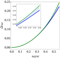
Figure 1: Paul trap effective energy $\hbar\Omega$ (a) and effective mass $M$ (b) as function of the drive’s frequency $\omega_{0}/\omega$ obtained from Eq. (31). The green solid curves show the exact results and the blue solid curves show the approximation at first order ($H_{0}\ll V$).

Example 2: Modulated optical lattice- The second-quantized tight-binding Hamiltonian of the modulated optical lattice Lignier et al. (2007); Goldman and Dalibard (2014) is given by

$$H=H_{0}+\omega\kappa\cos\left(\omega t\right)V,$$ (32)

where $\kappa$ is a constant parameter, $H_{0}=J\sum_{j}(a_{j+1}^{\dagger}a_{j}+a_{j}^{\dagger}a_{j+1})$ is the nearest-neighbor hopping term and $V=\sum_{j}ja_{j}^{\dagger}a_{j}$ is the lattice potential. The operators $a_{j}^{\dagger}$ and $a_{j}^{\dagger}$ are standard boson creation and annihilation operators at cite $j$. Following the procedure described above the effective Hamiltonian is found to be

$$H_{\mathrm{e}}=\Big{(}\beta_{1}(T)h_{1}+\beta_{2}(T)h_{2}+\beta_{3}(T)h_{3}\Big{)}/T=J_{0}(\kappa)H_{0},$$

where $\beta_{1}(T)=$ $\beta_{2}(T)=0,$ and $\beta_{3}(T)=TJ_{0}(\kappa)$. A detailed calculation of these parameters can be found in the SM. $H_{\mathrm{e}}$ is the same as the exact solution given in Ref. Goldman and Dalibard (2014).

Example 3: Kapitza pendulum- Here we examine the Hamiltonian of a harmonic oscillator subject to a time-dependent force Rahav et al. (2003)

$$H=\frac{p^{2}}{2m}+\frac{1}{2}m\omega_{0}^{2}x^{2}+xF\cos(\omega t).$$ (33)

In principle, the three elements in this Hamiltonian can be identified as part of the algebra formed by the operator set $h_{1}=1$, $h_{2}=x$, $h_{3}=p$ , $h_{4}=x^{2}$, $h_{5}=xp+px$, $h_{6}=p^{2}$ However, calculations are sizeabley simplified by choosing instead $h_{1}=1$, $h_{2}=x$, $h_{3}=p$ , $h_{4}=m^{2}\omega_{0}^{2}x^{2}+p^{2}$. The corresponding non-vanishing structure constants are $c_{2,3,1}=-c_{3,2,1}=1$, $c_{4,2,3}=-c_{2,4,3}=-2$, $c_{4,3,2}=-c_{3,4,2}=2m^{2}\omega_{0}^{2}$. By following the method, as detailed in the SM, the effective Hamiltonian is

$$H_{\mathrm{e}}=\Big{(}\beta_{1}(T)+\beta_{2}(T)x+\beta_{3}(T)p\\ +\beta_{4}(T)\left[p^{2}+(m\omega_{0})^{2}x^{2}\right]\Big{)}/T,$$ (34)

where $\beta_{1}(T)$, $\beta_{2}(T)$, $\beta_{3}(T)$ and $\beta_{4}(T)$ are explicitly given in the SM. This Hamiltonian can be rewritten in a more familiar form by eliminating the terms proportional to $x$ and $p$ via the unitary transformation $U\equiv U_{2}(\beta_{3}/2\beta_{4})U_{3}(-\beta_{2}/2(m\omega_{0})^{2}\beta_{4})=\exp(i\hbar x\beta_{3}/2\beta_{4})\exp(-i\hbar p\beta_{2}/2(m\omega_{0})^{2}\beta_{4})$. The transformed effective Hamiltonian takes the form

$$H^{\prime}_{e}=UH_{\mathrm{e}}U^{\dagger}=\frac{p^{2}}{2m}+\frac{1}{2}m\omega_{0}^{2}x^{2}+\frac{F^{2}}{4m\left(\omega^{2}-\omega_{0}^{2}\right)}.$$ (35)

Though this effective Hamiltonian has not been determined explicitly before, (35) is consistent with its very well known quasienergies Rahav et al. (2003).

In conclusion, we have presented a general method to find the time evolution operator and the effective Hamiltonian for time-driven systems using an algebraic approach. Then we reproduced the solutions for known exact solvable models, while we solved the Paul trap model.

This work was supported by DCB UAM-A grant numbers 2232214 and 2232215, and UNAM DGAPA PAPIIT IN102717. J.C.S.S. has a scholarship from Becas de Posgrado UAM number 2151800745.