The Supersymmetric R-Parity Violating Dine-Fischler-Srednicki-Zhitnitsky Axion Model

Abstract

We propose a complete R-parity violating supersymmetric model with baryon triality that contains a Dine-Fischler-Srednicki-Zhitnitsky axion chiral superfield. We parametrize supersymmetry breaking with soft terms, and determine under which conditions the model is cosmologically viable. As expected we always find a region of parameter space in which the axion is a cold dark matter candidate. The mass of the axino, the fermionic partner of the axion, is controlled by a Yukawa coupling. When heavy [${\cal O}$(TeV)], the axino decays early and poses no cosmological problems. When light [$\mathcal{O}$(keV)] it can be long lived and a warm dark matter candidate. We concentrate on the latter case and study in detail the decay modes of the axino. We find that constraints from astrophysical X- and gamma rays on the decay into photon and neutrino can set new bounds on some trilinear supersymmetric R-parity violating Yukawa couplings. In some corners of the parameter space the decays of a relic axino can also explain a putative 3.5 keV line.

1 Introduction

Supersymmetry (SUSY) is the best candidate to explain the hierarchy problem of the Standard Model (SM) [1, 2], and thus a leading candidate for the discovery of new physics effects at the LHC. Most supersymmetric models which have been searched for at the LHC make the assumption of conserved R-parity [3]. A very restrictive and widely considered version with universal boundary conditions at the unification scale, the constrained minimal supersymmetric Standard Model (CMSSM) [4], is now in considerable tension with collider data [5]. The R-parity violating (RpV) CMSSM is still very much allowed [6].

R-parity is a discrete multiplicative symmetry invoked in the CMSSM to forbid baryon and lepton number violating operators which together lead to rapid proton decay. The bonus of imposing R-parity is that the lightest supersymmetric particle (LSP), typically the neutralino, is stable and provides a dark matter (DM) candidate in the form of a weakly interacting massive particle (WIMP). This is the most popular and most searched for DM candidate. However, to–date no neutralino dark matter has been found [7, 8, 9]. It is thus prudent to investigate other DM candidates, also within alternative supersymmetric models.

R-parity does not forbid some dimension-5 operators dangerous for proton decay [10]. This issue can be resolved by imposing a $Z_{6}$ discrete symmetry, known as proton hexality (P₆), which leads to the same renormalizable superpotential as R-parity [11, 12], but is incompatible with a GUT symmetry. Alternatively, one can impose a $Z_{3}$–symmetry known as baryon-triality (B₃) [11, 13, 14, 15, 16, 17, 18]. The latter allows for lepton number violating operators in the superpotential thanks to which the neutrinos acquire Majorana masses, without introducing a new very high energy Majorana mass scale [19, 15, 16, 17, 20, 21, 22, 23, 24]. This is a virtue of B₃ models.​ A possible handicap is that the LSP is unstable and is not a dark matter candidate. This can be naturally resolved when taking into account the strong CP problem, as we discuss in the following.

Besides the hierarchy problem, every complete model should also address the strong CP problem [30], which plagues the SM, as well as its supersymmetric generalizations. In its simplest forms this necessitates introducing the pseudo scalar axion field [31, 32]. In the supersymmetric versions, the axion is part of a chiral supermultiplet and is accompanied by another scalar, the saxion, and a spin-1/2 fermion, the axino.

In this paper we propose to study a B₃ model with the inclusion of an axion supermultiplet of the Dine-Fischler-Srednicki-Zhitnitsky (DFSZ) type [33, 34]. The axion contributes to the DM energy density in the form of cold DM [35, 36]. Depending on the value of its decay constant, $f_{a}$, it constitutes all or a fraction of the DM. The gravitino is heavy [${\cal O}({\rm TeV})$], decays early in the history of the universe, and does not pose cosmological problems. The axino mass is proportional to $\lambda_{\chi}v_{\chi}$ [see Eq. (2.18)], where $v_{\chi}$ is the vacuum expectation value (VEV) of a scalar field of the order of the soft masses [${\cal O}$(TeV)], and $\lambda_{\chi}$ is a dimensionless Yukawa coupling in the superpotential. We consider two cases: (i) a heavy axino ($\sim$ TeV, which requires $\lambda_{\chi}\sim 1$), and (ii) a light one ($\sim$ keV, requiring ${\bf\lambda}_{\chi}\ll 1$). In case (i) the axino decays early and is not a DM candidate. In the more interesting case (ii), it is the LSP, its lifetime is longer than the age of the universe, and contributes as warm DM [37]. We study in detail its three decay channels: into an axion and a neutrino, into three neutrinos, into a neutrino and a photon, the last one subject to constraints from X- and gamma-ray data.

In 2014 a potential anomaly was observed in X-ray data coming from various galaxy clusters and the Andromeda galaxy [38, 39]. There have been several papers discussing this in terms of an axino in R-parity violating supersymmetry [40, 41, 42]. Although we were able to show that this explanation is not probable [43].

The outline of the paper is as follows. In Sec. 2, we introduce the model, describe its parameters and mass spectrum. In Sec. 3 we compute in detail the axino decay rates and branching fractions. In Sec. 4 we consider cosmological and astrophysical constraints on the model, with a focus on the more interesting case of a light axino. We conclude with a discussion of our results and point out possible future directions of investigation.

In Appendix A we include some general comments on the axino mass, we discuss its dependence on the SUSY breaking scale and point out that DFSZ models accommodate more easily a light axino, as opposed to models à la Kim-Shifman-Vainshtein-Zakharov (KSVZ) [44, 45]. In Appendix B we furthermore give details on the derivation of the mixings of the axino mass eigenstates.

2 The RpV DFSZ Supersymmetric Axion Model

2.1 The Lagrangian

Superfield	SU(3)C	SU(2)L	U(1)Y	U(1)${}_{\text{P}Q}~{}$
$\hat{Q}$	$3$	$2$	$1/6$	$Q_{Q}$
$\hat{\bar{U}}$	$\bar{3}$	$1$	$-2/3$	$Q_{\bar{U}}$
$\hat{\bar{D}}$	$\bar{3}$	$1$	$1/3$	$Q_{\bar{D}}$
$\hat{L}$	$1$	$2$	$-1/2$	$Q_{L}$
$\hat{\bar{E}}$	$1$	$1$	$1$	$Q_{\bar{E}}$
$\hat{H}_{d}$	$1$	$2$	$-1/2$	$Q_{H_{d}}$
$\hat{H}_{u}$	$1$	$2$	$1/2$	$Q_{H_{u}}$
$\hat{A}$	$1$	$1$	$0$	$Q_{A}$
$\hat{\bar{A}}$	$1$	$1$	$0$	$-Q_{A}$
$\hat{\chi}$	$1$	$1$	$0$	$0$

Table 1: Charge assignments for the chiral superfields. Note in our R-parity violating supersymmetric models $Q_{H_{d}}=Q_{L}$.

The building blocks of the minimal supersymmetric DSFZ axion model are the particle content of the MSSM plus three superfields, which are necessary to construct a self-consistent axion sector as discussed in Ref. [46]. The particle content, the quantum numbers with respect to the SM gauge sector $SU(3)_{c}\times SU(2)_{L}\times U(1)_{Y}$, and the charges under the global Peccei-Quinn (PQ) symmetry [47], $U(1)_{\rm PQ}$, are summarized in Table 1. The renormalizable superpotential is given by

$$W =W_{B_{3}}+W_{I}+W_{\rm PQ}\,,$$ (2.1)

$$W_{B_{3}} =Y_{u}\hat{Q}\hat{H}_{u}\hat{\bar{U}}+Y_{d}\hat{Q}\hat{H}_{d}\hat{\bar{D}}+Y_{e}\hat{L}\hat{H}_{d}\hat{\bar{E}}+\frac{1}{2}\lambda\hat{L}\hat{L}\hat{\bar{E}}+\lambda^{{}^{\prime}}\hat{L}\hat{Q}\hat{\bar{D}}\,,$$ (2.2)

$$W_{I} =c_{1}\hat{A}\hat{H}_{u}\hat{H}_{d}+c_{2}\hat{A}\hat{L}\hat{H}_{u}\,,$$ (2.3)

$$W_{\rm PQ} =\lambda_{\chi}\hat{\chi}\left(\hat{A}\hat{\bar{A}}-\frac{1}{4}f_{a}^{2}\right)\,.$$ (2.4)

Here and in the following we suppress generation, as well as isospin and color indices. Superfields are denoted by a hat superscript. We have imposed the discrete $Z_{3}$ symmetry [11] known as baryon triality, $B_{3}$. This leaves only the RpV operators $\frac{1}{2}{\bf\lambda}\hat{L}\hat{L}\hat{\bar{E}}$, $\lambda^{{}^{\prime}}\hat{L}\hat{Q}\hat{\bar{D}}$, and $c_{2}\hat{A}\hat{L}\hat{H}_{u}$. We have generalized the usual bilinear operators $\mu H_{u}H_{d}$ and $\kappa_{i}L_{i}H_{u}$ to obtain PQ invariance. The PQ charges satisfy

$$Q_{A}+Q_{H_{u}}+Q_{H_{d}}=0\,,\quad Q_{A}+Q_{H_{u}}+Q_{L}=0\,,$$ (2.5)

from the terms in Eq. (2.3), and similar relations for the other fields that are readily obtained from the terms in the rest of the superpotential.

The PQ symmetry is spontaneously broken at the scale $f_{a}$, due to scalar potential resulting from $W_{\rm PQ}$, and the scalar parts of $\hat{A}$ and $\hat{\bar{A}}$ get vacuum expectation values (VEVs) $v_{A},\,v_{\bar{A}}$, respectively,

$$A=\frac{1}{\sqrt{2}}\left(\phi_{A}+i\sigma_{A}+v_{A}\right)\,,\hskip 28.45274pt\bar{A}=\frac{1}{\sqrt{2}}\left(\phi_{\bar{A}}+i\sigma_{\bar{A}}+v_{\bar{A}}\right)\,.$$ (2.6)

The VEVs must fulfill

$$v_{A}\cdot v_{\bar{A}}=\frac{1}{2}f_{a}^{2}\,,$$ (2.7)

and we denote their ratio as

$$\tan^{2}\beta^{\prime}\equiv\frac{v_{\bar{A}}}{v_{A}}\,.$$ (2.8)

Below the PQ breaking scale, we generate an effective $\mu$-term, $\mu_{\rm eff}\hat{H}_{u}\hat{H}_{d}$, and effective bilinear RpV $\kappa$-terms, $\kappa_{\rm eff,i}\hat{L}_{i}\hat{H}_{u}$, with

$$\mu_{\rm eff}=\frac{c_{1}}{\sqrt{2}}v_{A}\,,\hskip 28.45274pt\kappa_{\rm eff,i}=\frac{c_{2,i}}{\sqrt{2}}v_{A}\,.$$ (2.9)

For successful spontaneous breaking of the electroweak (EW) symmetry, $\mu_{\rm eff}$ should be of the order of the EW scale, while $\kappa_{\rm eff}$ is constrained by neutrino physics, as discussed below, and should be $\leq O(\text{MeV})$. Since $f_{a}>10^{9}$ GeV from astrophysical bounds on axions [48], the couplings $c_{1}$ and $c_{2}$ must be very small, roughly $c_{1}<10^{-6}$ and $c_{2}<10^{-11}$. They are, nonetheless, radiatively stable.

We have assumed that $W_{\rm PQ}$ respects an $R$-symmetry, under which the field $\hat{\chi}$ has charge 2. This forbids the superpotential terms $\hat{\chi}^{2}$ and $\hat{\chi}^{3}$. See also Ref. [25].

The soft-supersymmetric terms of this model consist of scalar squared masses, gaugino masses, and the counterparts of the superpotential couplings. The full soft Lagrangian reads

$$-\mathcal{L}_{\rm soft}= (M_{1}\widetilde{B}\widetilde{B}+M_{2}\widetilde{W}\widetilde{W}+M_{3}\widetilde{g}\widetilde{g}+{\rm h.c.})+\widetilde{f}^{\dagger}m^{2}_{\widetilde{f}}\widetilde{f}$$

$$+m^{2}_{\chi}|\chi|^{2}+m^{2}_{{A}}|A|^{2}+m^{2}_{\bar{{A}}}|\bar{A}|^{2}+m^{2}_{H_{u}}|H_{u}|^{2}+m^{2}_{H_{d}}|H_{d}|^{2}+m^{2}_{\ell H_{u}}(\widetilde{\ell}^{\dagger}H_{u}+H_{u}^{\dagger}\widetilde{\ell})$$

$$+\left(B\mu H_{d}\cdot H_{u}+\rm h.c.\right)+(T_{u}\widetilde{u}\widetilde{q}H_{u}+T_{d}\widetilde{d}\widetilde{q}H_{d}+T_{e}\widetilde{e}\widetilde{\ell}H_{d}+T_{\lambda}\widetilde{\ell}\widetilde{\ell}\widetilde{e}+T_{\lambda^{{}^{\prime}}}\widetilde{\ell}\widetilde{q}\widetilde{d}$$

$$+T_{c1}AH_{u}H_{d}+T_{c2}A\,\widetilde{\ell}H_{u}+T_{\lambda_{\chi}}\,\chi A\bar{A}+L_{V}\chi+{\rm h.c.})\;,$$ (2.10)

with $\widetilde{f}\in\{\widetilde{e},\widetilde{\ell},\widetilde{d},\widetilde{u},\widetilde{q}\}$. We assume that SUSY breaking violates the $R$-symmetry of the axion sector, hence we include the soft terms $T_{\lambda_{\chi}}\,\chi A\bar{A}$ and $L_{V}\chi$. Note that, even if set to zero at some scale, these terms would be generated at the two-loop level because of the small coupling to the MSSM sector, where no $R$-symmetry is present.

At low energy the Lagrangian contains interactions of the axion with the gauge fields. These are best understood by performing a field rotation that leads to a basis in which all the matter fields are invariant under a PQ transformation [50]. We have

$$\mathcal{L}_{aVV}=\frac{a}{32\pi^{2}f_{a}}\left(g_{1}^{2}C_{aBB}B_{\mu\nu}\widetilde{B}^{\mu\nu}+g_{2}^{2}C_{aWW}W^{a}_{\mu\nu}\widetilde{W}^{a\mu\nu}+g_{3}^{2}G^{\alpha}_{\mu\nu}\widetilde{G}^{\alpha\mu\nu}\right)\,.$$ (2.11)

Here $a$ is the axion field which in our model is given by $a\simeq\frac{1}{\sqrt{2}}(\sigma_{A}-\sigma_{\bar{A}})$ to a good approximation​​, cf. Eq. (2.6). $B_{\mu\nu}$, $W^{a}_{\mu\nu}$, $G^{a}_{\mu\nu}$ are the SM field strength tensors, here $a$ is an adjoint gauge group index, with $\widetilde{X}^{a\mu\nu}\equiv\epsilon^{\mu\nu\rho\sigma}X^{a}_{\rho\sigma}$, and the coefficients are given in terms of the PQ charges

$$C_{aBB} =3(3Q_{Q}+Q_{L})-7Q_{A}\,,$$ (2.12)

$$C_{aWW} =-3(3Q_{Q}+Q_{L})+Q_{A}\,.$$ (2.13)

In the supersymmetric limit the couplings of the axino to gauginos and gauge fields are related to those in Eq. (2.11). We are, however, interested in the case of broken SUSY. In general, such axino couplings can be calculated explicitly, by computing triangle loop diagrams, once the full Lagrangian is specified, as it is in our model. Later in the paper we use the full Lagrangian to compute the one-loop decay of the axino into a photon and a neutrino, including the couplings.

2.2 The Mass Spectrum

We now turn our attention to the spin-1/2 neutral fermion mass spectrum of this model. The $10\times 10$ mass matrix in the basis $(\lambda_{\widetilde{B}},\widetilde{W}^{0},\widetilde{H}_{u}^{0},\widetilde{H}_{d}^{0},\nu_{L,i},\widetilde{A},\widetilde{\bar{A}},\widetilde{\chi})$, which is a generalization of the MSSM neutralino mass matrix, reads

$$\mathcal{M}_{\chi^{0}}=\left[\begin{array}[]{cccccccccc}M_{1}&0&\frac{g_{1}v_{u}}{2}&-\frac{g_{1}v_{d}}{2}&0&0&0&0&0&0\\ 0&M_{2}&-\frac{g_{2}v_{u}}{2}&\frac{g_{2}v_{d}}{2}&0&0&0&0&0&0\\ \frac{g_{1}v_{u}}{2}&-\frac{g_{2}v_{u}}{2}&0&-\frac{c_{1}v_{A}}{\sqrt{2}}&\frac{c_{2,1}v_{A}}{\sqrt{2}}&\frac{c_{2,2}v_{A}}{\sqrt{2}}&\frac{c_{2,3}v_{A}}{\sqrt{2}}&-\frac{c_{1}v_{d}}{\sqrt{2}}&0&0\\ -\frac{g_{1}v_{d}}{2}&\frac{g_{2}v_{d}}{2}&-\frac{c_{1}v_{A}}{\sqrt{2}}&0&0&0&0&-\frac{c_{1}v_{u}}{\sqrt{2}}&0&0\\ 0&0&\frac{c_{2,1}v_{A}}{\sqrt{2}}&0&0&0&0&\frac{c_{2,1}v_{u}}{\sqrt{2}}&0&0\\ 0&0&\frac{c_{2,2}v_{A}}{\sqrt{2}}&0&0&0&0&\frac{c_{2,2}v_{u}}{\sqrt{2}}&0&0\\ 0&0&\frac{c_{2,3}v_{A}}{\sqrt{2}}&0&0&0&0&\frac{c_{2,3}v_{u}}{\sqrt{2}}&0&0\\ 0&0&-\frac{c_{1}v_{d}}{\sqrt{2}}&-\frac{c_{1}v_{u}}{\sqrt{2}}&\frac{c_{2,1}v_{u}}{\sqrt{2}}&\frac{c_{2,2}v_{u}}{\sqrt{2}}&\frac{c_{2,3}v_{u}}{\sqrt{2}}&0&\frac{v_{\chi}\lambda_{\chi}}{\sqrt{2}}&\frac{v_{\bar{A}}\lambda_{\chi}}{\sqrt{2}}\\ 0&0&0&0&0&0&0&\frac{v_{\chi}\lambda_{\chi}}{\sqrt{2}}&0&\frac{v_{A}{\bf\lambda}_{\chi}}{\sqrt{2}}\\ 0&0&0&0&0&0&0&\frac{v_{\bar{A}}\lambda_{\chi}}{\sqrt{2}}&\frac{v_{A}{\bf\lambda}_{\chi}}{\sqrt{2}}&0\\ \end{array}\right]\,.$$ (2.14)

$\mathcal{M}_{\chi^{0}}$ was obtained by first implementing our model with the computer program SARAH [51, 52, 53], then setting the sneutrino VEVs to zero, which corresponds to choosing a specific basis [54, 55]. This is possible, since the superfields $\hat{H}_{d}$ and $\hat{L}_{i}$ have the same quantum numbers in RpV models. The choice of basis is scale dependent, in the sense that sneutrino VEVs are generated by renormalization group (RG) running, even if set to zero at a given scale. Hence, one needs to specify at what scale the basis is chosen. For later convenience, when we compute the axino decays, we choose this scale to be the axino mass. Neglecting for a moment the axino sector, which couples very weakly to the rest, and Takagi diagonalizing the upper-left $7\times 7$ block [56], one finds [20, 57] two massless neutrinos and a massive one with

$$m_{\nu}\approx m_{Z}\cos^{2}\beta\sin^{2}\xi\approx m_{Z}\cos^{2}\beta\ \frac{\kappa_{\rm eff}^{2}}{\mu_{\rm eff}^{2}}\,,$$ (2.15)

where

$$\tan\beta=\frac{v_{u}}{v_{d}}\,,\quad\mathrm{and}\quad\cos\xi=\frac{\mu_{\rm eff}}{\sqrt{\mu_{\rm eff}^{2}+\kappa_{\rm eff,1}^{2}+\kappa_{\rm eff,2}^{2}+\kappa_{\rm eff,3}^{2}}}\,.$$ (2.16)

Requiring $m_{\nu}\approx 0.1$ eV, with $\tan\beta\approx 1$ and $\mu_{\rm eff}\approx 1$ TeV, one finds that $\kappa_{\rm eff,i}$ is of order MeV, and correspondingly smaller for larger $\tan\beta$. The two neutrinos which are massless at tree level acquire a small mass at one loop [23, 24, 19], which we have not included in the 10x10 mass matrix above.

In addition to the neutrinos, there are four eigenstates, mainly built from the MSSM neutralinos $(\lambda_{\widetilde{B}},\widetilde{W}^{0},\widetilde{H}_{u}^{0},\widetilde{H}_{d}^{0})$, with masses between 100 and 1000 GeV, and three axino eigenstates with masses that can be calculated analytically in the limit $v_{A}=v_{\bar{A}}=\frac{f_{a}}{\sqrt{2}}$, corresponding to $\tan\beta^{\prime}=1$, and $c_{1,2}\to 0$. One finds for the axinos [46]

$$-\frac{1}{\sqrt{2}}\lambda_{\chi}v_{\chi}\,,\ \ \frac{1}{2\sqrt{2}}\Big{(}\lambda_{\chi}v_{\chi}\pm\lambda_{\chi}\sqrt{v_{\chi}^{2}+4f_{a}^{2}}\Big{)}\,.$$ (2.17)

The lightest of these three states corresponds to the fermionic component of the linear combination of superfields $\frac{1}{\sqrt{2}}(\bar{A}-A)$. It is interpreted as the axino with a mass [46]

$$m_{\widetilde{a}}\simeq-\frac{1}{\sqrt{2}}\lambda_{\chi}v_{\chi}\,.$$ (2.18)

For the more general case of $\tan\beta^{\prime}\neq 1$, we can not give analytical expressions. Instead, we find at the lowest order in $v_{\chi}/f_{a}$

$$m_{\widetilde{a}}\simeq-\frac{\sqrt{2}\tan^{2}\beta^{\prime}}{1+\tan^{4}\beta^{\prime}}\lambda_{\chi}v_{\chi}+{\cal O}\left(\lambda_{\chi}v_{\chi}\frac{v_{\chi}^{2}}{f_{a}^{2}}\right)\,.$$ (2.19)

We also give the power of the next term in the expansion, where $f_{a}$ enters. This is the main contribution to the axino mass, we neglect small corrections proportional to $c_{1}$ and $c_{2}$. We expect $v_{\chi}$ to be at the soft SUSY breaking scale, ${\cal O}$(TeV). The Yukawa coupling ${\bf\lambda}_{\chi}$ then is our main parameter to control $m_{\widetilde{a}}$. $\lambda_{\chi}$ is radiatively stable: if we set it small at tree level, it remains small. See also Ref. [58] for a quantitative treatment of Yukawa RGEs inn supersymmetric models. The most interesting case we consider later is that of a light axino, with $m_{\widetilde{a}}={\cal O}$(keV), which means ${\bf\lambda}_{\chi}$ must be very small.

In order to determine the interactions of the axino, in particular the potential decay modes, we would like to estimate the mixing between the axino and the neutrinos. To do this one first diagonalizes the upper 7x7 block, neglecting the axinos which are very weakly coupled. The massive neutrino eigenstate will be mostly a combination of the gauge eigenstates $\nu_{L,i}$, with small components of bino, wino and higgsinos. Next include the lower 3x3 axino block. The off-diagonal entries between the neutrino and axino blocks are $c_{2}v_{u}/\sqrt{2}\simeq\kappa_{\rm eff}v_{u}/f_{a}$. Now rotate the 3x3 axino block to the mass eigenstates. The axino is a linear combination of $A$ and $\bar{A}$, the other two heavier fermions are a combination of $A$, $\bar{A}$ and $\chi$. The important point is that the entries in the 3x3 Takagi diagonalization axino matrix are of order one. This implies that the pieces in the off diagonal blocks remain of order $\kappa_{\rm eff}v_{u}/f_{a}$ after rotating the axino block, and we obtain the form of the matrix

$$\mathcal{M}_{\widetilde{a},\nu}=\begin{bmatrix}m_{\nu}&{\cal O}\left(\frac{\kappa_{\rm eff}v}{f_{a}}\right)\\ {\cal O}\left(\frac{\kappa_{\rm eff}v}{f_{a}}\right)&m_{\widetilde{a}}\end{bmatrix}\,.$$ (2.20)

From this we can read off the axino-neutrino mixing

$$x_{\widetilde{a},\nu}\approx\frac{\kappa_{\rm eff}v}{m_{\widetilde{a}}f_{a}}\,.$$ (2.21)

For the purpose of this estimate and those in Sec. 4, we take $v\equiv\sqrt{v_{u}^{2}+v_{d}^{2}}\sim v_{u}\sim v_{d}$ to be the weak scale.

The axino-higgsino mixing can be estimated by observing that the higgsino mass is of order $\mu_{\rm eff}$, and the off-diagonal element between axino and higgsino is of order $c_{1}v=\frac{\mu_{\rm eff}}{f_{a}}v$. Thus, the mixing is

$$x_{\widetilde{a},\widetilde{H}}\approx\frac{c_{1}v}{\mu_{\rm eff}}=\frac{v}{f_{a}}\,.$$ (2.22)

Considering $M_{1}\sim\mu_{\rm eff}\sim M_{\rm SUSY}={\cal O}$(TeV), we can estimate the bino-higgsino mixing as $g_{1}\frac{v}{M_{\rm SUSY}}$. Multiplying this times $x_{\widetilde{a},\widetilde{H}}$ we obtain the axino-bino mixing

$$x_{\widetilde{a},\widetilde{B}}\approx g_{1}\frac{v^{2}}{M_{\rm SUSY}f_{a}}\,.$$ (2.23)

Next we briefly consider the scalar sector. It is instructive to start by considering the limit $c_{1,2}\rightarrow 0$, in which there is no mixing between the MSSM sector and the axion sector, and the axion block of the scalar squared mass matrix can easily be diagonalized. We find a massless axion and a saxion with a mass squared $\sim m_{A}^{2}$ or $m_{\bar{A}}^{2}$, the parameters in the soft Lagrangian [$m_{A},\,m_{\bar{A}}={\cal O}$(TeV), cf. Eq. (2.10)]. They are, respectively, the CP-odd and the CP-even mass eigenstates, corresponding to the combination $\frac{1}{\sqrt{2}}(\bar{A}-A)$. The result is not appreciably altered once we turn on the small couplings $c_{1}$ and $c_{2}$. The other four real scalar degrees of freedom in this sector are heavy, with masses of order $\lambda_{\chi}f_{a}$. The masses of the scalars in the MSSM sector are to a very good approximation those already well studied in the RpV SUSY literature [19, 58].

3 Light Axino Decay Modes

In this section we consider an axino mass lower than twice the electron mass, in which case the axino has only three three decay modes:

1. into a neutrino and an axion (via a dimension 5 operator), $\tilde{a}\to\nu_{i}+a$;

2. into three neutrinos (tree-level), $\tilde{a}\to\nu_{i}+\nu_{j}+\nu_{k}$;

3. into a neutrino and a photon (one-loop), $\tilde{a}\to\nu_{i}+\gamma$.

We discuss them in turn.

3.1 Decay into Neutrino and Axion

The dominant operator responsible for the decay $\tilde{a}\to a+\nu$ is dimension 5:

$$\frac{1}{f_{a}}(\partial^{\mu}a)\bar{\psi}_{\tilde{a}}\gamma_{\mu}\gamma_{5}\psi_{\tilde{a}}\,.$$ (3.1)

This is in the basis of the mass matrix in Eq. (2.20), before we diagonalize to the final mass eigenstate. Here $a$ is the axion, $\psi_{\tilde{a}}$ is the four-component spinor denoting the axino mass eigenstate and the neutrino arises due to mixing with the axino, once we diagonalize. A simple way to understand the origin of this operator is to consider the kinetic term $\bar{\psi}_{\tilde{a}}\gamma_{\mu}\partial^{\mu}\psi_{\tilde{a}}$. After the chiral rotation $\psi_{\tilde{a}}\to e^{i\gamma_{5}a/f_{a}}\psi_{\tilde{a}}$, we obtain the above operator, when we expand the exponential. The diagram for the decay is shown in Fig. 1a, where we include the axino-neutrino mixing [see Eq. (2.21)] in the final state. The partial decay width into this channel is

$$\Gamma_{\tilde{a}\to\nu a} =\frac{x_{\tilde{a},\nu}^{2}}{16\pi}\frac{m_{\widetilde{a}}^{3}}{f_{a}^{2}}\approx\frac{1}{16\pi}\frac{v_{u}^{2}\kappa_{\rm eff}^{2}}{f_{a}^{4}}m_{\widetilde{a}}$$ (3.2)

$$=6\cdot 10^{-54}\ {\rm GeV}\left(\frac{\kappa_{\rm eff}}{\rm MeV}\right)^{2}\left(\frac{10^{11}\ {\rm GeV}}{f_{a}}\right)^{4}\left(\frac{m_{\widetilde{a}}}{\rm keV}\right)\,.$$ (3.3)

(a)

(b)

Figure 1: Left: Feynman diagram for the axino decay into an axion and a neutrino, as described by the five-dimensional operator of Eq. (3.1). Right: One of the Feynman diagrams describing the decay of the axino into three neutrinos. In our convention the $\otimes$ on a fermion line stands for a mixing between fermionic eigenstates.

3.2 Decay into Three Neutrinos

This tree-level decay proceeds via the axino mixing with the neutrino and the exchange of a Z boson between the fermionic currents, as shown in Fig. 1b. Assuming for simplicity that the neutrino admixture of the axino is measured by $x_{{\widetilde{a}},\nu}$ for all neutrino flavors, the decay width into all possible flavors of final neutrinos reads [59]

$$\Gamma_{\tilde{a}\to 3\nu} =\frac{9\alpha G_{F}^{2}}{8\pi^{4}}x_{\tilde{a},\nu}^{2}m_{\widetilde{a}}^{5}$$ (3.4)

$$=3\cdot 10^{-56}\ {\rm GeV}\ \left(\frac{\kappa_{\rm eff}}{\rm MeV}\right)^{2}\left(\frac{10^{11}\ {\rm GeV}}{f_{a}}\right)^{2}\left(\frac{m_{\widetilde{a}}}{\rm keV}\right)^{3}\,.$$ (3.5)

$\Gamma_{\tilde{a}\to 3\nu}$ and $\Gamma_{\tilde{a}\to\nu a}$ give the main contribution to the total decay width in most of the parameter space. We find that for $10^{10}\ {\rm GeV}<f_{a}<10^{12}\ {\rm GeV}$ and $1\ {\rm keV}<m_{\widetilde{a}}<100\ {\rm keV}$, the axino lifetime ranges from $10^{23}$ to $10^{41}$ s, which is longer than the age of the universe ($\sim 4\cdot 10^{17}$ s).

3.3 Decay into Photon Plus Neutrino

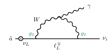
(a)

(b)

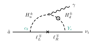
(c)

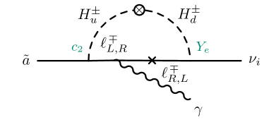
(d)

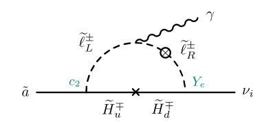
(e)

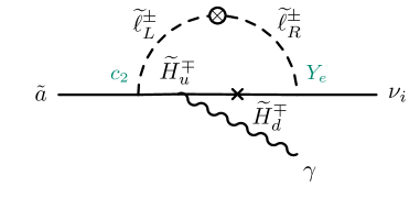
(f)

Figure 2: Diagrams with no dependence on the the RpV trilinear couplings $\lambda^{(\prime)}$. The cross on a fermion line indicates a mass insertion needed for the chirality flip, while the $\otimes$ on a scalar or fermion line is a (dimensionless) mixing. We write the coupling constants in green at the vertices.

The one-loop diagrams for the decay $\widetilde{a}(p)\to\nu(k_{1})+\gamma(k_{2})$ have an amplitude with the following structure [60] dictated by gauge invariance

$${\cal M}=ig_{\widetilde{a}\nu\gamma}\bar{u}(k_{1})\left(P_{R}-\eta_{\nu}\eta_{\widetilde{a}}P_{L}\right)\sigma^{\mu\nu}k_{2\mu}\epsilon^{*}_{\nu}u(p)\,.$$ (3.6)

Here $\eta_{\nu}$ and $\eta_{\widetilde{a}}$ are the signs of the mass eigenvalues of the neutrino and the axino, respectively, $k_{2}$ the photon momentum, and $\epsilon$ its polarization vector. $g_{\widetilde{a}\nu\gamma}$ is a function with the details of the loop integrals, and has the dimension of inverse mass. The decay rate then has the form

$$\Gamma_{\widetilde{a}\to\nu\gamma}=\frac{|g_{\tilde{a}\nu\gamma}|^{2}m_{\widetilde{a}}^{3}}{16\pi}\,.$$ (3.7)

We are neglecting the final state neutrino mass. The corresponding Feynman diagrams are shown in Figs. 2 and 3. Here we are interested in an estimate, and thus wish to determine which diagram(s) is (are) dominant. Thus we first consider the individual amplitudes squared, in turn, as well as the corresponding decay width, without including interference terms. If not otherwise specified, we make use of the formulae provided in Ref. [61] to compute the loop integrals. We do not include diagrams with sneutrino VEVs insertions (see e.g. Ref. [62]), since, as previously mentioned, we work in the basis, defined at the axino mass scale, where such VEVs are zero.

The first diagrams we consider are those depicted in Fig. 2a , 2b. The corresponding decay width has been computed in the analogous case of a sterile neutrino decaying into a neutrino and a photon [63] (see also Ref. [64] for a review),

$$\Gamma_{\nu(Wl)} =\frac{9\alpha G_{F}^{2}}{1024\pi^{4}}x_{\tilde{a},\nu}^{2}m_{\widetilde{a}}^{5}\approx\frac{9\alpha G_{F}^{2}}{1024\pi^{4}}\frac{\kappa_{\rm eff}^{2}v_{u}^{2}}{f_{a}^{2}}m_{\widetilde{a}}^{3}$$ (3.8)

$$=3\cdot 10^{-58}\ {\rm GeV}\ \left(\frac{\kappa_{\rm eff}}{\rm MeV}\right)^{2}\left(\frac{10^{11}\ {\rm GeV}}{f_{a}}\right)^{2}\left(\frac{m_{\widetilde{a}}}{\rm keV}\right)^{3}\,.$$

Here, the first subscript on $\Gamma$ indicates the state the incoming axino mixes with, while the subscripts in parentheses denote the particles running in the loop. We use this notation for the rest of the section. Let us anticipate that in most of the parameter space we consider, $\Gamma_{\nu(Wl)}$ gives the dominant contribution. It is therefore useful to compare the other partial widths to $\Gamma_{\nu(Wl)}$. Incidentally, a decay width of $\Gamma_{\tilde{a}}=3\cdot 10^{-58}\,$GeV corresponds to a lifetime $\tau_{\tilde{a}}=2\cdot 10^{23}\,$s and the lifetime of the universe is about $\tau_{\mathrm{univ.}}\approx 4\cdot 10^{17}\,$s.

The main contribution to the two diagrams in Fig. 2c, 2d comes from the heaviest lepton that can run in the loop, the $\tau$. We have

$$\Gamma_{(Hl)}\approx\frac{m_{\widetilde{a}}^{3}}{2^{11}\pi^{5}}\frac{\kappa_{\rm eff}^{2}}{f_{a}^{2}}\left(\frac{B\mu}{m_{H^{\pm}}^{2}}\right)^{2}Y_{\tau}^{2}\frac{m_{\tau}^{2}}{m_{H^{\pm}}^{4}}\ln^{2}\left(\frac{m_{\tau}^{2}}{m_{H^{\pm}}^{2}}\right)\,.$$ (3.9)

The $m_{\tau}^{2}$ in the numerator comes from the mass insertion that flips the chirality in the fermion line in the loop, while $B\mu/m_{H^{\pm}}^{2}$ is an estimate of the mixing between the charged scalar Higgses, $B\mu$ being the bilinear parameter in the Higgs potential, see Eq. (2.10). Taking $B\mu\sim m_{H^{\pm}}^{2}$ as an estimate, we find the ratio

$$\frac{\Gamma_{(Hl)}}{\Gamma_{\nu(Wl)}} =\frac{1}{18\pi\alpha G_{F}^{2}}\frac{Y_{\tau}^{2}}{v_{u}^{2}}\frac{m_{\tau}^{2}}{m_{H^{\pm}}^{4}}\ln^{2}\left(\frac{m_{\tau}^{2}}{m_{H^{\pm}}^{2}}\right)$$ (3.10)

$$\approx 3\cdot 10^{-8}\left(\frac{m_{H^{\pm}}}{{\rm TeV}}\right)^{-4}\frac{\ln^{2}\left(\frac{m_{\tau}^{2}}{m_{H^{\pm}}^{2}}\right)}{160}\,,$$

which is highly suppressed, and we neglect the contributions from the corresponding diagrams in the following.

Next we consider the diagrams of Fig. 2e, 2f. We assume the $\tilde{\tau}$ to be the lightest charged slepton and give the leading contribution. We find

$$\Gamma_{(\tilde{H}\tilde{l})}\approx\frac{m_{\widetilde{a}}^{3}}{2^{12}\pi^{5}}\frac{\kappa_{\rm eff}^{2}}{f_{a}^{2}}x_{\tilde{\tau}_{LR}}^{2}Y_{\tau}^{2}\frac{\mu_{\rm eff}^{2}}{m_{\tilde{\tau}}^{4}}\frac{\left(1+\ln\frac{\mu_{\rm eff}^{2}}{m_{\tilde{\tau}}^{2}}-\frac{\mu_{\rm eff}^{2}}{m_{\tilde{\tau}}^{2}}\right)^{2}}{\left(1-\frac{\mu_{\rm eff}^{2}}{m_{\tilde{\tau}}^{2}}\right)^{4}}\,.$$ (3.11)

Here, $x_{\tilde{\tau}_{LR}}$ is the mixing between the left and right staus, $\mu_{\rm eff}$ is the Higgsino mass. Note that the expression is finite in the limit $\mu_{\rm eff}=m_{\tilde{\tau}}$. Taking $x_{\tilde{\tau}_{LR}}\approx 1$, we find the ratio

$$\frac{\Gamma_{(\tilde{H}\tilde{l})}}{\Gamma_{\nu(Wl)}} =\frac{1}{18\pi\alpha G_{F}^{2}}\frac{Y_{\tau}^{2}}{v_{u}^{2}}\frac{\mu_{\rm eff}^{2}}{m_{\tilde{\tau}}^{4}}\frac{\left(1+\ln\frac{\mu_{\rm eff}^{2}}{m_{\tilde{\tau}}^{2}}-\frac{\mu_{\rm eff}^{2}}{m_{\tilde{\tau}}^{2}}\right)^{2}}{\left(1-\frac{\mu_{\rm eff}^{2}}{m_{\tilde{\tau}}^{2}}\right)^{4}}$$ (3.12)

$$\approx 10^{-5}\left(\frac{\mu_{\rm eff}}{{\rm TeV}}\right)^{2}\left(\frac{m_{\tilde{\tau}}}{{\rm TeV}}\right)^{-4}\,.$$

This is also highly suppressed and we neglect it in the following.

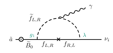
(a)

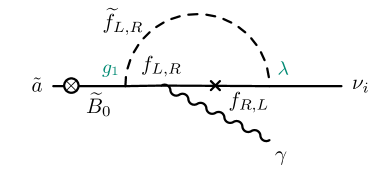
(b)

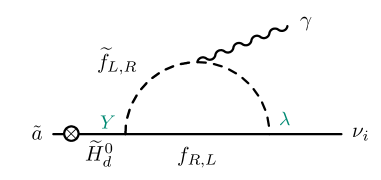
(c)

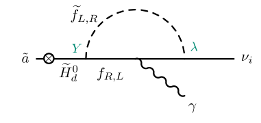
(d)

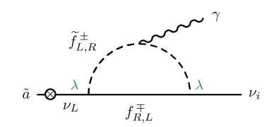
(e)

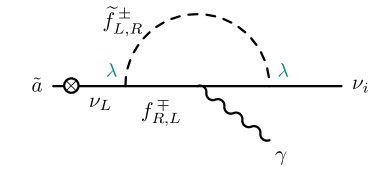
(f)

Figure 3: Diagrams with an explicit dependence on the RpV trilinear couplings $\lambda^{(\prime)}$. The notation is as in Fig. 2.

Next, we examine the diagrams of Fig. 3, which involve at least one trilinear RpV coupling, $\lambda$ or $\lambda^{\prime}$. To avoid cluttering the equations, we use $\lambda$ to denote either. For the diagrams of Fig. 3a , 3b we find

$$\Gamma_{\widetilde{B}\left(f\tilde{f}\right)}\approx\frac{m_{\widetilde{a}}^{3}Q^{2}_{f}}{2^{11}\pi^{5}}g_{1}^{2}\lambda^{2}x_{\widetilde{a},\widetilde{B}}^{2}\frac{m_{f}^{2}}{m_{\widetilde{f}}^{4}}\ln^{2}\left(\frac{m_{f}^{2}}{m_{\widetilde{f}}^{2}}\right)\,.$$ (3.13)

Here, $f$ ($\widetilde{f}$) denotes either a down-type quark (squark), in the case of a ${\bf\lambda}^{\prime}$ coupling, or a lepton (slepton), in the case of a ${\bf\lambda}$ coupling. $Q_{f}$ is the electric charge of $f$ in units of $e$, and $g_{1}=e/\cos\theta_{W}$ is the hypercharge gauge coupling. The dominant contributions come from loops of bottom-sbottom, or tau-stau; the two are of the same order of magnitude, under the assumption that sleptons and squarks have comparable masses, as the smaller mass of $\tau$ is compensated by its larger electric charge. The axino-bino mixing is estimated in Eq. (2.23). Comparing this contribution to the one of Eq. (3.8), we find

$$\frac{\Gamma_{\widetilde{B}\left(f\tilde{f}\right)}}{\Gamma_{\nu\left(Wl\right)}} =\frac{g_{1}^{4}Q^{2}}{18\pi\alpha G_{F}^{2}}\frac{\lambda^{2}v^{2}}{M_{\rm SUSY}^{2}\kappa_{\rm eff}^{2}}\frac{m_{f}^{2}}{m_{\widetilde{f}}^{4}}\ln^{2}\left(\frac{m_{f}^{2}}{m_{\widetilde{f}}^{2}}\right)$$ (3.14)

$$\approx 0.2\left(\frac{\lambda}{10^{-2}}\right)^{2}\!\left(\frac{Q_{f}}{1/3}\right)^{2}\left(\frac{{\rm MeV}}{\kappa_{\rm eff}}\right)^{2}\left(\frac{{\rm TeV}}{M_{\rm SUSY}}\right)^{2}\left(\frac{m_{f}}{m_{b}}\right)^{2}\left(\frac{{\rm TeV}}{m_{\widetilde{f}}}\right)^{4}\frac{\ln^{2}\left(\frac{m_{f}^{2}}{m_{\widetilde{f}}^{2}}\right)}{120}\,,$$

where $m_{b}$ is the mass of the bottom quark. For sfermions lighter than a TeV, $\Gamma_{\widetilde{B}\left(f\tilde{f}\right)}$ would give a contribution larger than $\Gamma_{\nu\left(Wl\right)}$. Here we restrict ourselves to $m_{\widetilde{f}}>1$ TeV, motivated by recent analyses [65, 6], which disfavor lighter squarks and sleptons. We comment further on this contribution below.

For the diagrams of Fig. 3c , 3d we find (note there is no mass insertion in the fermion line in the loop)

$$\Gamma_{\widetilde{H}\left(f\tilde{f}\right)}\approx\frac{m_{\widetilde{a}}^{3}Q^{2}_{f}}{2^{11}\pi^{5}}Y^{2}\lambda^{2}x_{\widetilde{a},\widetilde{H}}^{2}\frac{m_{\widetilde{a}}^{2}}{m_{\widetilde{f}}^{4}}\ln^{2}\left(\frac{m_{f}^{2}}{m_{\widetilde{f}}^{2}}\right)\,.$$ (3.15)

Here, $f$ ($\widetilde{f}$) can be either a down-type quark (squark), in the case of a ${\bf\lambda}^{\prime}$ coupling, or a lepton (slepton), in the case of a ${\bf\lambda}$ coupling. $Y$ is either the $Y_{d}$ or the $Y_{e}$ Yukawa, and the axino-higgsino mixing is given in Eq. (2.22). As in the previous case, the main contributions to these diagrams are from bottom-sbottom and tau-stau loops, respectively. $\Gamma_{\widetilde{H}\left(f\tilde{f}\right)}$ is suppressed compared to $\Gamma_{\widetilde{B}\left(f\tilde{f}\right)}$ by a factor $m_{\widetilde{a}}^{2}/m_{f}^{2}$. We have

$$\frac{\Gamma_{\widetilde{H}\left(f\tilde{f}\right)}}{\Gamma_{\nu\left(Wl\right)}} =\frac{Q^{2}_{f}}{18\pi\alpha G_{F}^{2}}\frac{\lambda^{2}Y^{2}}{\kappa_{\rm eff}^{2}}\frac{m_{\widetilde{a}}^{2}}{m_{\widetilde{f}}^{4}}\ln^{2}\left(\frac{m_{f}^{2}}{m_{\widetilde{f}}^{2}}\right)$$ (3.16)

$$\approx 10^{-12}\left(\frac{\lambda}{10^{-2}}\right)^{2}\left(\frac{Q_{f}}{1/3}\right)^{2}\left(\frac{Y}{Y_{b}}\right)^{2}\left(\frac{{\rm MeV}}{\kappa_{\rm eff}}\right)^{2}\left(\frac{m_{\widetilde{a}}}{10\ {\rm keV}}\right)^{2}\left(\frac{{\rm TeV}}{m_{\widetilde{f}}}\right)^{4}\frac{\ln^{2}\left(\frac{m_{f}^{2}}{m_{\widetilde{f}}^{2}}\right)}{120}\,.$$

The last two diagrams to evaluate are those of Fig. 3e, 3f. The two RpV couplings appearing in each of these diagrams have no restrictions on their flavor index structure, contrary to those of Figs. 3a to 3d, which are diagonal in the singlet-doublet mixings. For the sake of our discussion we also do not distinguish between the two potentially different $\lambda$ here, as we consider only one RpV coupling to be different from zero at a time. We find

$$\Gamma_{\nu\left(f\tilde{f}\right)}\approx\frac{m_{\widetilde{a}}^{3}Q^{2}_{f}}{2^{11}\pi^{5}}\lambda^{4}x_{\widetilde{a}\widetilde{\nu}}^{2}\frac{m_{\widetilde{a}}^{2}}{m_{\widetilde{f}}^{4}}\ln^{2}\left(\frac{m_{f}^{2}}{m_{\widetilde{f}}^{2}}\right)\,,$$ (3.17)

the main contributions being again from bottom-sbottom and tau-stau loops, and

$$\frac{\Gamma_{\nu\left(f\tilde{f}\right)}}{\Gamma_{\nu\left(Wl\right)}} =\frac{Q^{2}_{f}}{18\pi\alpha G_{F}^{2}}\frac{\lambda^{4}}{m_{\widetilde{f}}^{4}}\left(\log\frac{m_{f}^{2}}{m_{\widetilde{f}}^{2}}\right)^{2}$$ (3.18)

$$\approx 10^{-9}\left(\frac{\lambda}{10^{-2}}\right)^{4}\left(\frac{Q_{f}}{1/3}\right)^{2}\left(\frac{{\rm TeV}}{m_{\widetilde{f}}}\right)^{4}\frac{\ln^{2}\left(\frac{m_{f}^{2}}{m_{\widetilde{f}}^{2}}\right)}{120}\,.$$

From our estimates we see that $\Gamma_{\widetilde{B}\left(f\tilde{f}\right)}$ and $\Gamma_{\nu(Wl)}$ give the dominant contributions, the other diagrams being always negligible. Thus the axion decay width into photon and neutrino is given to a good approximation by $\Gamma_{\widetilde{B}\left(f\tilde{f}\right)}+\Gamma_{\nu(Wl)}$. In Fig. 4 we plot the branching ratios corresponding to the three decay channels of our light axino.

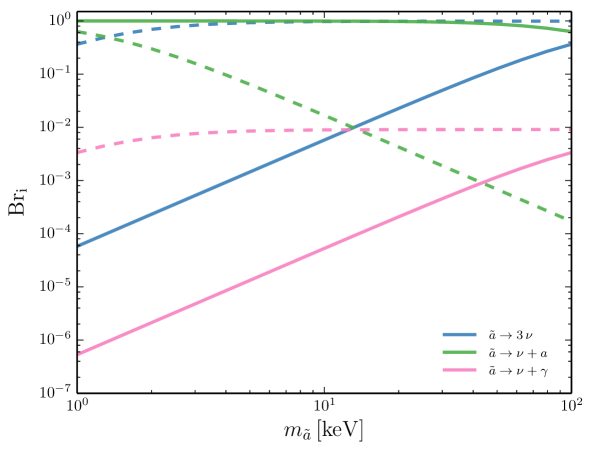
Figure 4: We show the branching ratios of the axino decay channels into axion and neutrino, three neutrinos, photon and neutrino, as a function of the axino mass. The total width is $\Gamma_{\tilde{a}\to a\nu}+\Gamma_{\tilde{a}\to 3\nu}+\Gamma_{\tilde{a}\to\gamma\nu}$, where in $\Gamma_{\tilde{a}\to\gamma\nu}$ we take into account only the two dominant contributions, $\Gamma_{\widetilde{B}\left(f\tilde{f}\right)}+\Gamma_{\nu(Wl)}$, as discussed in the main text. We consider a loop of bottom-sbottom for the evaluation of $\Gamma_{\widetilde{B}\left(f\tilde{f}\right)}$, with $m_{\tilde{b}}=1$ TeV (the tau-stau contribution would be analogous) and the RpV trilinear coupling $\lambda=10^{-2}$. Continuous (dashed) lines are for $f_{a}=10^{10}$ GeV ($f_{a}=10^{12}$ GeV).

It is worth examining $\Gamma_{\widetilde{B}\left(f\tilde{f}\right)}$ in more detail. First, we reintroduce the generation indices in the superpotential terms

$$\frac{1}{2}\lambda_{ijk}\hat{L}_{i}\hat{L}_{j}\hat{\bar{E}}_{k}+\lambda^{{}^{\prime}}_{ijk}\hat{L}_{i}\hat{Q}_{j}\hat{\bar{D}}_{k}\,.$$ (3.19)

As the main contributions to $\Gamma_{\widetilde{B}\left(f\tilde{f}\right)}$ are from tau-stau and bottom-sbottom loops, the trilinear couplings of interest are those shown in Table 2. The first index of $\lambda_{ijk}$ and $\lambda^{{}^{\prime}}_{ijk}$ refers, in our case, to the neutrino in the lepton doublet. We see in Fig. 5 that when we consider the decay $\widetilde{a}\to\nu_{2}\gamma$, with $\lambda_{233}$ and $\lambda^{{}^{\prime}}_{233}$ saturating the upper bounds in Table 2, the diagrams giving $\Gamma_{\widetilde{B}\left(f\tilde{f}\right)}$ provide the dominant contribution.

We can use this fact to set new bounds on these trilinear couplings by considering constraints from X and gamma rays [66, 67] on the decays $\widetilde{a}\to\nu_{2,3}\gamma$. We proceed as follows. First, we assume that the entire dark matter is constituted by the axino, $\Omega_{\widetilde{a}}h^{2}=\Omega_{\rm DM}$. This fixes $f_{a}$ for any given value of $m_{\widetilde{a}}$. Then the excluded region corresponds to

$$\Gamma_{\widetilde{B}\left(f\tilde{f}\right)}>\Gamma_{\rm bound}=\frac{1}{\tau_{\rm bound}}\,,$$ (3.20)

where $\tau_{\rm bound}$ is given, for instance, in Fig. 9 of Ref. [67] as a function of the mass of the decaying particle, the axino in our case. In Fig. 6 we see that, for $m_{\widetilde{a}}=100$ keV, we can set bounds on the trilinears $\lambda_{233},\lambda^{{}^{\prime}}_{233},\lambda^{{}^{\prime}}_{333}$ of order $10^{-2}$. These are to be compared with the bounds in Table 2. However, it is important to keep in mind that these new bounds, contrary to those in Table 2, rely on the presence of the axino and on the assumption that it is the whole dark matter.

ijk	$\lambda_{ijk}(M_{W})$	$\lambda^{\prime}_{ijk}(M_{W})$
133	$0.0060\times\sqrt{\frac{m_{\tilde{\tau}}}{$100\text{\,}\mathrm{G}\mathrm{e}\mathrm{V}$}}$	$0.0014\times\sqrt{\frac{m_{\tilde{b}}}{$100\text{\,}\mathrm{G}\mathrm{e}\mathrm{V}$}}$
233	$0.070\times\frac{m_{\tilde{\tau}_{R}}}{$100\text{\,}\mathrm{G}\mathrm{e}\mathrm{V}$}$	$0.15\times\sqrt{\frac{m_{\tilde{b}}}{$100\text{\,}\mathrm{G}\mathrm{e}\mathrm{V}$}}$
333	-	$0.45\ (1.04)$

Table 2: Upper bounds on the magnitude of R-parity violating couplings at the $2\sigma$ confidence level, taken from Ref. [6]. The constraints arise from indirect decays. The concrete processes are described in detail in Ref. [68].

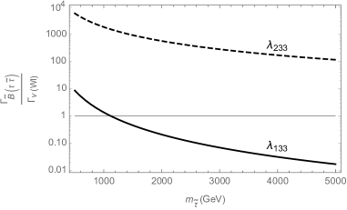
(a)

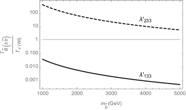
(b)

Figure 5: We show the ratio $\frac{\Gamma_{\widetilde{B}\left(f\tilde{f}\right)}}{\Gamma_{\nu\left(Wl\right)}}$ from Eq. (3.14) as a function of the sfermion mass. We have set $M_{\rm SUSY}=1$ TeV and $\kappa_{\rm eff}=1$ MeV. The left plot corresponds to the tau-stau loop, with $m_{f}=m_{\tau}$. The solid line is obtained by taking $\lambda=\lambda_{133}=0.006\sqrt{\frac{m_{\tilde{\tau}}}{100\ {\rm GeV}}}$, while for the dashed line $\lambda=\lambda_{233}=0.07\frac{m_{\tilde{\tau}}}{100\ {\rm GeV}}$. The right plot corresponds to the bottom-sbottom loop, with $m_{f}=m_{b}$. The solid line is obtained by taking $\lambda^{{}^{\prime}}=\lambda^{{}^{\prime}}_{133}=0.0014\sqrt{\frac{m_{\tilde{b}}}{100\ {\rm GeV}}}$, while for the dashed line $\lambda=\lambda^{{}^{\prime}}_{233}=0.15\sqrt{\frac{m_{\tilde{b}}}{100\ {\rm GeV}}}$. The values chosen for the trilinear couplings saturate the up-to-date bounds of Table 2.

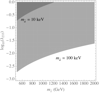
(a)

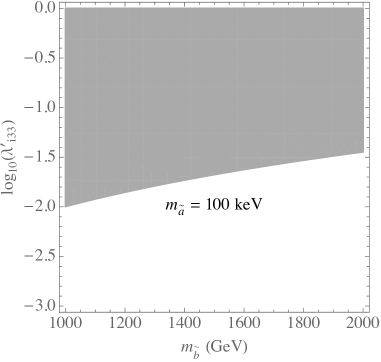
(b)

Figure 6: We show regions excluded by X and gamma-ray constraints [66, 67]. Here we use Eq. (3.20) and assume the axino to contribute to the totality of dark matter. The dark (light) gray region is excluded when $m_{\widetilde{a}}=10$ keV (100 keV). In $\lambda^{{}^{\prime}}_{i33}$, the index $i$ can be either 2 or 3, in which case the dominant contribution to the decay $\widetilde{a}\to\nu_{i}\gamma$ is from $\Gamma_{\widetilde{B}\left(f\tilde{f}\right)}$.

In Fig. 8 we show the X and gamma-ray constraints on the plane $f_{a}$ vs $m_{a}$. The excluded regions in purple correspond to

$$\frac{\Omega_{\widetilde{a}}}{\Omega_{\rm DM}}\Gamma_{\widetilde{a}\to\nu\gamma}>\Gamma_{\rm bound}=\frac{1}{\tau_{\rm bound}}\,.$$ (3.21)

Here, $\Gamma_{\widetilde{a}\to\nu\gamma}={\rm max}[\Gamma_{\widetilde{B}\left(f\tilde{f}\right)},\Gamma_{\nu\left(Wl\right)}]$, and we multiply by $\Omega_{\widetilde{a}}/\Omega_{\rm DM}$ to account for the region of parameter space where the axino is under abundant. We discuss the axino relic abundance in Sec. 4.

3.4 Comment on the 3.5 keV Line.

This model can fit the 3.5 keV line observed in galaxy clusters [38, 39, 42, 40]. A possible benchmark point, for instance, is the following:

$$m_{\widetilde{a}}=7\ {\rm keV}\,,\ f_{a}=3.5\cdot 10^{10}\ {\rm GeV}\,,\ m_{\widetilde{b}}=2\ {\rm TeV}\,,\ \lambda^{\prime}_{233}=0.22\,.$$ (3.22)

With these values, the axino constitutes the entire dark matter and has a partial decay width $\Gamma_{\widetilde{a}\to\nu\gamma}\approx\Gamma_{\widetilde{B}\left(f\tilde{f}\right)}\approx 6\cdot 10^{-53}$ GeV, needed to explain the putative line. The benchmark complies with the bounds we mentioned above. We emphasize, however, that evidence that the 3.5 keV line is due to decaying DM is not conclusive [69, 70, 71, 72, 73, 74, 75, 76, 77].

4 Cosmological and Astrophysical Constraints

4.1 The Gravitino

We assume a supergravity completion of our model, with SUSY broken at a high scale ($\sqrt{F}\sim 3\cdot 10^{10}$ GeV) and the breaking effects mediated via Planck suppressed operators, so that the soft scale is $M_{\rm SUSY}\sim\frac{F}{M_{\rm Pl}}={\cal O}$(TeV). The gravitino is heavy, with $m_{3/2}\sim M_{\rm SUSY}$, decays before BBN, and poses no cosmological problems.

4.2 The Saxion

In the context of supersymmetric axion models one usually has to worry about the saxion: if it is too light it can pose serious issues (see e.g. Ref. [78]). We briefly review why. The saxion is a pseudomodulus, meaning that its potential is quite flat. During inflation we expect it to sit at a distance of order $f_{a}$ from the minimum of its zero-temperature potential. After inflation, when the Hubble parameter $H$ becomes comparable to the saxion mass, $m_{s}$, the saxion starts to oscillate about its minimum. From the condition $H(T_{s}^{\rm osc})\sim m_{s}$, with $H(T)\sim\frac{T^{2}}{M_{\rm Pl}}$, we find the temperature at which the oscillations start

$$T_{s}^{\rm osc}\sim\sqrt{m_{s}M_{\rm Pl}}\,.$$ (4.1)

At that time the energy density in the oscillating field is $\rho_{s}\sim m_{s}^{2}f_{a}^{2}$. The energy density of radiation is $\rho_{r}\sim(T_{s}^{\rm osc})^{4}$, so that $\left(\frac{\rho_{s}}{\rho_{r}}\right)_{\rm osc}\sim\frac{f_{a}^{2}}{M_{\rm Pl}^{2}}$. The energy density of the oscillating saxion scales as $T^{3}$, behaving like matter, which implies that in the absence of decays it would come to dominate the energy density of the universe at a temperature

$$T_{s}^{\rm dom}\sim\frac{f_{a}^{2}}{M_{\rm Pl}^{2}}T_{s}^{\rm osc}\sim\frac{f_{a}^{2}}{M_{\rm Pl}^{2}}\sqrt{m_{s}M_{\rm Pl}}\,.$$ (4.2)

It is important to determine whether it decays before or after domination. To proceed with this simple estimate we parametrize the decay rate as $\Gamma_{s}\sim\frac{1}{16\pi}\frac{m_{s}^{3}}{f_{a}^{2}}$, neglecting the masses of the decay products. The factor of $f_{a}^{2}$ at the denominator is due to the fact that the saxion couplings to matter are suppressed by $f_{a}$. Then the decay temperature is obtained from $H(T_{s}^{\rm dec})\sim\Gamma_{s}$:

$$T_{s}^{\rm dec}\sim\frac{m_{s}^{3/2}M_{\rm Pl}^{1/2}}{10f_{a}}\,.$$ (4.3)

From these estimates we find

$$\frac{T_{s}^{\rm dec}}{T_{s}^{\rm dom}}\sim 10^{4}\left(\frac{m_{s}}{1\ {\rm TeV}}\right)\left(\frac{10^{12}\ {\rm GeV}}{f_{a}}\right)^{3}\,.$$ (4.4)

In our model the saxion mass is of order TeV, so it decays way before it comes to dominate the energy density of the universe. Note the temperature when it decays is of order GeV, safely above BBN.

4.3 Axion Dark Matter

In this model the axion is a dark matter candidate. We do not review here the calculations of its relic abundance, but refer the reader to Ref. [81, 82]. There are two important mechanisms to produce axion cold DM. One is the misalignment mechanism, which results in the abundance

$$\Omega_{a,\rm mis}h^{2}=0.18\ \theta_{1}^{2}\left(\frac{f_{a}}{10^{12}\ {\rm GeV}}\right)^{1.19}\left(\frac{\Lambda_{\rm QCD}}{400\ {\rm MeV}}\right)\,,$$ (4.5)

with $\theta_{1}$ the initial misalignment angle. The other contribution comes from axions emitted by global axionic strings, which also contribute as non-relativistic axions:

$$\Omega_{a,{\rm str}}h^{2}\approx 0.2\ \xi\ \bar{r}\left(\frac{f_{a}}{10^{12}\ {\rm GeV}}\right)^{1.19}\left(\frac{\Lambda_{\rm QCD}}{400\ {\rm MeV}}\right)\,.$$ (4.6)

Here $\xi$ is the length parameter which represents the average number of strings in a horizon volume. It is determined by numerical simulations [83], $\xi\simeq 1.0$. The parameter $\bar{r}$ is related to the average energy of the axions emitted in string decays. Its value has been the subject of a long debate. Two scenarios have been put forth, one predicts $\bar{r}\approx 1$, the other $\bar{r}\approx 70$. See Ref. [84] and references therein for details, and Ref. [85] for recent considerations on the issue.

While the misalignment mechanism produces axions when the temperature is $T\sim\Lambda_{\rm QCD}$, the strings form at a much higher temperature $T\sim f_{a}$. If the PQ phase transition happened before the end of inflation, or equivalently if the reheating temperature ($T_{\rm RH}$) were lower than $f_{a}$, then the strings would be inflated away and we would no longer have a contribution corresponding to Eq. (4.6). In this scenario the axion abundance is from Eq. (4.5), and $\theta_{1}$ can take any value between $-\pi$ and $\pi$. In the scenario with the PQ phase transition post inflation ($T_{\rm RH}>f_{a}$), one has to average $\theta_{1}^{2}$ over many QCD horizons, $\langle\theta_{1}^{2}\rangle=\pi^{2}/3$, and the contribution from string decays can be comparable to that from misalignment or larger, depending on the value of $\bar{r}$.

4.4 A Heavy Axino

For $\lambda_{\chi}\sim 1$, we have $m_{\widetilde{a}}\sim v_{\chi}\sim M_{\rm SUSY}$, an axino mass of order TeV. Such an axino has many open decay channels into MSSM particles, with a total width that can be estimated as $\Gamma_{\widetilde{a}}\sim\frac{1}{8\pi}\frac{m_{\widetilde{a}}^{3}}{f_{a}^{2}}$. It decays safely before BBN, and does not pose cosmological issues.

4.5 A Light Axino

The axino, if light, can also be a dark matter candidate [37, 86, 87, 88, 89, 90, 91]. It was pointed out in Ref. [37] that for $T_{\rm RH}>f_{a}$ a stable axino should not exceed the mass of 1 or 2 keV, otherwise it would result in overabundant DM. More recently Bae et al. [82, 92] showed that the axino production rate is suppressed if $M_{\Phi}\ll f_{a}$, where $M_{\Phi}$ is the mass of the heaviest PQ–charged and gauge–charged matter supermultiplet in the model. This suppression is significant in DFSZ models, where $M_{\Phi}$ corresponds to the Higgsino mass. The consequence of such a suppression is that the upper bound of 2 keV on the axino mass quoted in Ref. [37] is relaxed. In our model the axino is not stable. However, if its mass is below the electron mass the only decay modes are

1. into a neutrino and an axion (tree-level, with dimension 5 operator), $\tilde{a}\to\nu_{i}+a$;

2. into three neutrinos (tree-level), $\tilde{a}\to\nu_{i}+\nu_{j}+\nu_{k}$;

3. into a neutrino and a photon (one-loop), $\tilde{a}\to\nu_{i}+\gamma$.

The resulting lifetime, as we show in the following subsections, is longer than the age of the universe, thus making the axino a dark matter candidate, with relic abundance

$$\Omega_{\widetilde{a}}h^{2}\simeq 2.1\times 10^{-5}\left(\frac{m_{\widetilde{a}}}{1\ {\rm keV}}\right)\left(\frac{10^{12}\ {\rm GeV}}{f_{a}}\right)^{2}\,.$$ (4.7)

This does not depend on $T_{\rm RH}$, as long as $T_{\rm RH}>10^{4}$ GeV [82, 92]. For lower $T_{\rm RH}$ and different cosmological histories the axion abundance can be different [93], but we will not consider such scenarios in this work. We learn that, for $f_{a}=10^{12}$ GeV, the axino can have a mass as large as a few MeV before it becomes overabundant. The important feature of Eq. (4.7) is that the abundance is inversely proportional to $f_{a}^{2}$. It is easy to understand why. The axino never reaches thermal equilibrium in the early universe because its interactions are very weak. It is produced in scattering processes (listed e.g. in Table 1 of Ref. [82]) with a cross section proportional to $1/f_{a}^{2}$. The larger the cross section the more the axino is produced, hence the $1/f_{a}^{2}$ dependence in Eq. (4.7). In Fig. 7 we show the allowed region of parameter space, in the plane $f_{a}$ vs $m_{\widetilde{a}}$, where we can have both axion and axino dark matter.

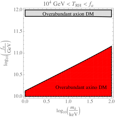
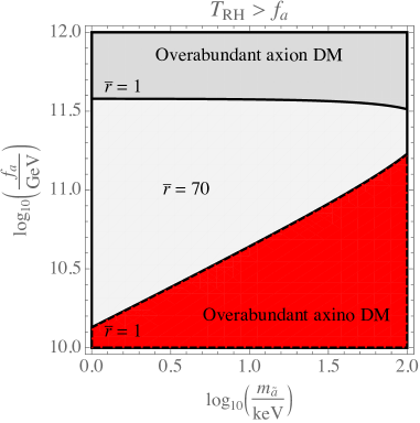
Figure 7: We show, in the plane $f_{a}$ vs the axino mass $m_{\widetilde{a}}$, the regions where the combination of axion and the axino dark matter exceeds the observed abundance, $(\Omega_{a}+\Omega_{\widetilde{a}})h^{2}>\Omega_{\rm DM}h^{2}=0.12$ [94]. In the grey region the main contribution is from the axion, in the red from the axino [Eq. (4.7)]. Along the black solid line the axion alone results in the correct abundance, while along the black dashed line the axino alone accounts for $\Omega_{\rm DM}$. In the left panel the reheat temperature, $T_{\rm RH}$, is below the PQ phase transition scale, $f_{a}$, and the only contribution to axion dark matter is from the misalignment mechanism, Eq. (4.5). Here we take the initial misalignment angle $\theta_{1}=1$. In the white region, the combination of axion plus axino results in a total abundance below $\Omega_{\rm DM}$. In the right panel $T_{\rm RH}$ is above $f_{a}$, and we also have a contribution to axion dark matter from the decay of axionic strings, Eq. (4.6). We show the excluded region for two different values of the parameter $\bar{r}$. Note that for $\bar{r}=70$, axion plus axino are overabundant on the entire plane. Furthermore, the lifetime of the axino is longer than the age of the universe in the entire region plotted.

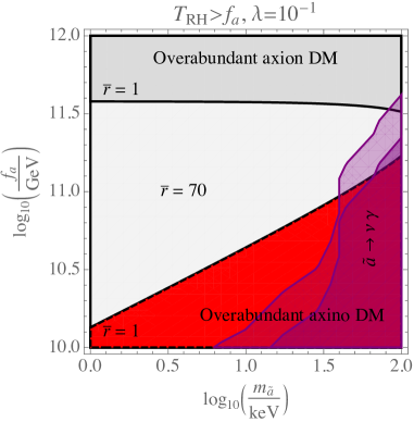
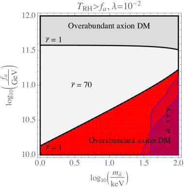
Figure 8: We add to the right plot of Fig. 7 the constraints from X and gamma rays [see Eq. (3.21)], shown in light purple. When these regions overlap with the red region, the parameter space is excluded by the overabundance of the axino. On the left we set the trilinear coupling to $\lambda=10^{-1}$, on the right $\lambda=10^{-2}$. The lighter (darker) purple region corresponds to a mass of the sfermion, running in the loop, of 1 (2) TeV.

5 Summary

We have presented for the first time a complete RpV SUSY model with baryon triality and with a DFSZ axion superfield. We have studied the mass spectrum and then investigated some cosmological bounds. The axion is a good dark matter candidate when its decay constant $f_{a}={\cal O}(10^{11})\,$GeV. For lower values of $f_{a}$ the axino, with a mass roughly between 1 and 100 keV, can be the dominant dark matter candidate. We have looked at the possible decay modes of the light axino in detail. For such a light axino, its lifetime is longer than the age of the universe, but its decay into photon and neutrino still leads to interesting phenomenology. We have shown that X- and gamma-ray constraints on this decay give new bounds on some trilinear RpV couplings. These are model dependent and rely on the axino constituting the whole dark matter in the universe. We have also shown that in this model there is a corner of parameter space where a 7 keV axino could fit the 3.5 keV line observed in galaxy clusters.

This model could be explored in further details in relation to neutrino physics or possible collider signatures. We leave it to future work.

Acknowledgements: We thank Branislav Poletanovic for helpful initial discussions, and Toby Opferkuch for comments on various aspects of this work. We thank Florian Staub for many very helpful discussions as well as his assistance in the use of SARAH. LU thanks Francesco D’Eramo for discussions and acknowledges support from the PRIN project “Search for the Fundamental Laws and Constituents” (2015P5SBHT_002). HKD would like to express a special thanks to the Mainz Institute for Theoretical Physics (MITP) for its hospitality and support during part of this work.

Appendix A The Unbearable Lightness of the Axino

The axino mass has been extensively discussed in the literature [95, 37, 96, 97, 98]. It is commonly held to be highly model dependent, taking on almost any value [87, 90]. In this appendix we point out that a keV mass axino is more easily embedded in the DFSZ class of models rather than in the KSVZ models [44, 45]. We then discuss how the mass is related to the PQ and SUSY breaking energy scales.

A.1 KSVZ vs DFSZ

Axion models fall into two broad categories denoted as KSVZ and DFSZ. Both contain a complex scalar field, $A(x)$, charged under a global $U(1)_{\rm PQ}$, PQ symmetry [47]. The axion field, $a(x)$, is identified with the phase of $A(x)$.​ In the KSVZ model, $A(x)$ couples to exotic heavy quark fields, $Q(x)$, that are charged under color and under the $U(1)_{\rm PQ}$ (and possibly $U(1)_{\mathrm{EM}}$), while the rest of the SM fields do not carry any PQ charge. The coupling $f_{Q}A\bar{Q}Q$ generates, via a triangle diagram, the interaction term $aG_{\mu\nu}\widetilde{G}^{\mu\nu}$ which is crucial in solving the strong CP problem. Here $G_{\mu\nu}(x)$ is the gluon field strength tensor and $\widetilde{G}^{\mu\nu}(x)$ its dual. In the supersymmetric version, the KSVZ model is defined by the superpotential $W_{\rm KSVZ}=f_{Q}\hat{A}\hat{\bar{Q}}\hat{Q}$, where we use hats to denote chiral superfields and $Q$, $\bar{Q}$ are two distinct superfields in the 3 and $\bar{\mathbf{3}}$ representations of $SU(3)_{c}$, respectively, but with equal PQ charge. Embedding the model in supergravity results in a one–loop contribution to the axino mass of order [99, 37]

$$m_{\widetilde{a}}\sim 10\ {\rm GeV}\left(\frac{m_{3/2}f^{2}_{Q}}{100\ {\rm GeV}}\right)\,,$$ (A.1)

where $m_{3/2}$ is the gravitino mass. Moreover, even if supergravity effects are neglected, there is an irreducible two-loop contribution involving the gluino [100]

$$m_{\widetilde{a}}\sim 0.3\ {\rm GeV}\left(\frac{m_{\widetilde{g}}f^{2}_{Q}}{1\ {\rm TeV}}\right)\,,$$ (A.2)

where $m_{\widetilde{g}}$ is the gluino mass. This implies that even if the axino mass is tuned to keV values at tree level, loop corrections tend to raise it to GeV values. Thus a KSVZ axino prefers to be heavier than a few keV.

In DFSZ models the field $A(x)$ couples to two Higgs doublets, $H_{u}$ and $H_{d}$, which are also charged under the $U(1)_{\rm PQ}$, as well as the other SM fields are. Thus the supersymmetric version of the DFSZ axion model is more economical than the KSVZ counterpart, as SUSY already requires at least two Higgs doublets. The SUSY coupling of axions to Higgses can be written as [37] $W_{\rm DFSZ}=c_{1}\hat{A}\hat{H}_{u}\hat{H}_{d}$. The field $A$ has to get a large vacuum expectation value (VEV) $\langle A\rangle\sim f_{a}$, with $f_{a}>10^{9}\,$GeV, otherwise the corresponding axion would be excluded by supernova constraints [48]. In turn, this implies a tiny coupling $c_{1}$. Note that the corresponding coupling in non supersymmetric DFSZ models also has to be very small, for the axion to be invisible. In the SUSY context it has been proposed that the operator $c_{1}\hat{A}\hat{H}_{u}\hat{H}_{d}$ could be replaced [101] by a non-renormalizable one $\frac{g}{M_{\rm Pl}}\hat{A}^{2}\hat{H}_{u}\hat{H}_{d}$. With the latter operator one easily obtains a $\mu$-term at the TeV scale, while with the former we are forced to take very small values the coupling $c_{1}$. We do not address the $\mu$-problem, but we point out that Ref. [102] showed that the operator we consider can be derived consistently within a string theory framework. The fact that $c_{1}$ is tiny helps with the axino mass: once we set it to keV values at tree level we are guaranteed that radiative corrections, proportional to $c_{1}$, will be negligible as opposed to the KSVZ case we discussed above.

A.2 Low-scale vs High-scale SUSY Breaking

In a previous paper [46], we indicated a simple way to understand that in models where the SUSY breaking scale, $M_{\rm SB}$, is lower than the PQ scale, $f_{a}$, the axino mass is of order $\mathcal{O}\left(\frac{M^{2}_{\rm SUSY}}{f_{a}}\right)$, with $M_{\rm SUSY}$ the scale of the soft supersymmetry breaking terms, while in models with $M_{\rm SB}>f_{a}$ the axino mass is typically of order $M_{\rm SUSY}$. The former models, with low $M_{\rm SB}$ are representative of global SUSY, for which the best known framework is gauge mediation of supersymmetry breaking [103]. The latter ones, with high $M_{\rm SB}$ usually fall in the scheme of gravity mediation of supersymmetry breaking, in local supersymmetry, and the scale of the soft terms is that of the gravitino mass, $M_{\rm SUSY}\sim m_{3/2}$.

In light of these considerations one would think that a light axino is more natural in the context of gauge mediation. However it turns out that this is difficult to accommodate. The problem is with the saxion. Consider a model of minimal gauge mediation (see e.g. Ref. [103]), where the messengers do not carry any PQ charge and communicate with the visible sector only via gauge interactions. The leading contribution to the mass of the sfermions of the minimal supersymmetric Standard Model (MSSM) is generated at two loops. However the saxion is a gauge singlet and its mass can only be generated at three loops, as shown schematically in Fig. 9.

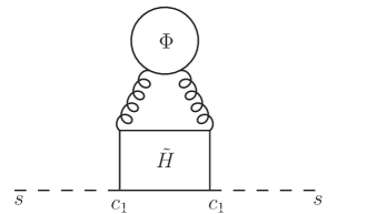
Figure 9: Three-loop contribution to the saxion mass in minimal gauge mediation. At the top we have a loop of messenger fields, $\Phi$, drawn as a circle, at the bottom a loop of Higgsinos, drawn as a rectangle. The wiggly lines are gauge bosons. The coupling $c_{1}$ of the saxion to the Higgsinos is defined in Eq. (2.3).

The coupling $c_{1}$ that appears twice in the diagram is the one we discussed in the previous subsection, and the same that appears in the superpotential of Eq. (2.1). The saxion squared mass, $m_{s}^{2}$ is suppressed by a factor of $\sim\frac{c_{1}^{2}}{16\pi^{2}}$ compared to the squared masses of the MSSM sfermions, $m_{\widetilde{f}}^{2}$, so we can estimate

$$m_{s}\sim 0.1\ {\rm keV}\ \left(\frac{c_{1}}{10^{-9}}\right)\left(\frac{m_{\widetilde{f}}}{1\ {\rm TeV}}\right)\,.$$ (A.3)

This light saxion could pose serious cosmological problems [104] as it would come to dominate the energy density of the universe for a long time before it decays. We reviewed some of the issues associated with saxion cosmology in Sec. 4. One way out of this problem would be to make the saxion heavier. This could be achieved by either coupling the axion superfield to the messengers or to fields in the hidden sector responsible for SUSY breaking. Apart from the extra field content that the procedure would bring into the model there is another issue that seems difficult to overcome: the same couplings needed to make the saxion heavier would very likely produce a heavy axino [105]. Perhaps there is a clever way to arrange for a heavy saxion and a light axino in gauge mediation, but in light of our considerations it seems that such a model would have to be quite complicated. We do not investigate this aspect further in this work. Rather we choose a supergravity (SUGRA) model. We showed in Ref. [46] that in SUGRA the axino would typically have a mass comparable to the gravitino, thus in the TeV range. However, we can adjust a single parameter, $\lambda_{\chi}$, to lower the axino mass down to the keV range. Doing so does not affect other masses, such as those of saxion and gravitino for instance. Also, as we argued above, since the axino we consider is of the DFSZ type, once we set its mass at tree level it will not be affected appreciably by loop corrections. Therefore the SUGRA model can be kept minimal, as opposed to a possible model with gauge mediation, at the expense of some tuning, needed to lower the mass of the axino. In the model presented in this paper the axino is much lighter than the gravitino. This represents an explicit exception to the generic argument that the axino should be heavier than the gravitino, put forward in Ref. [106].

Appendix B Axino-Gaugino Mixing

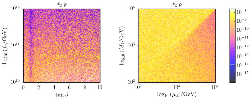
Figure 10: Distribution of the mixings $x_{\widetilde{a},\widetilde{B}}$ and $x_{\widetilde{a},\widetilde{H}}$ obtained by numerical evaluation of the eigenvalues of $\mathcal{M}_{4}$. We run $10^{5}$ points randomly varying $10^{2}\,{\rm GeV}\,<M_{1\,,2},\mu_{\rm eff}<10^{4}\,{\rm GeV}\,,\,1<\tan\beta<10\,,\,10^{10}\,{\rm GeV}<f_{a}<10^{12}\,{\rm GeV}\,,\,1\,{\rm keV}<m_{\widetilde{a}}<10^{2}\,{\rm keV}$. From our estimate in Eq. (2.22) [Eq. (2.23)] we expect $x_{\widetilde{a},\widetilde{H}}$ [$x_{\widetilde{a},\widetilde{B}}$] to lie somewhere in the range between approximately $10^{-10}$ and $10^{-8}$ GeV [$10^{-12}$ and $10^{-10}$ GeV], depending on the value of $f_{a}$.

Most of the amplitudes involved in the radiative decay of the axino bear a strong dependence on its mixing with some of the other neutralino mass eigenstates. In this work we rely on well-motivated estimates for these quantities, but in order to obtain their precise values one should diagonalize the neutralino mass matrix $\mathcal{M}_{\chi^{0}}$. While an exact analytical algorithm exists for the case of the MSSM [107], adding one more mass eigenstate, as for the case of the Next-to-Minimal Supersymmetric Standard Model (NMSSM), does not allow for a closed-form solution. In this section we show how the approximate block-diagonalization procedure of Ref. [108] for the NMSSM 5x5 neutralino mass matrix can be used to obtain a numerical value for the axino-gaugino mixing. The only requirement is a small mixing between the the singlet and the doublet states, which in our case corresponds to the mixing between any of the two Higgs doublets and the axion field $A$. From $\mathcal{M}_{\chi^{0}}$ in Eq. (2.14) we see that such mixing is indeed small, since $\frac{c_{1}v_{u,d}}{\sqrt{2}}\approx\frac{\mu_{\rm eff}}{f_{a}}\lesssim 10^{-7}$. Recalling that the axino mass eigenstate consists of a linear combination of the fermionic components of the fields $A$ and $\bar{A}$ only, we define the following neutralino mass 5x5 sub-matrix:

$$\mathcal{M}_{5} =\left[\begin{array}[]{ccccc}M_{1}&0&\frac{g_{1}v_{u}}{2}&-\frac{g_{1}v_{d}}{2}&0\\ 0&M_{2}&-\frac{g_{2}v_{u}}{2}&\frac{g_{2}v_{d}}{2}&0\\ \frac{g_{1}v_{u}}{2}&-\frac{g_{2}v_{u}}{2}&0&-\frac{c_{1}v_{A}}{\sqrt{2}}&-\frac{c_{1}v_{d}}{\sqrt{2}}\\ -\frac{g_{1}v_{d}}{2}&\frac{g_{2}v_{d}}{2}&-\frac{c_{1}v_{A}}{\sqrt{2}}&0&-\frac{c_{1}v_{u}}{\sqrt{2}}\\ 0&0&-\frac{c_{1}v_{d}}{\sqrt{2}}&-\frac{c_{1}v_{u}}{\sqrt{2}}&m_{\widetilde{a}}\\ \end{array}\right]\,,$$ (B.6)

where the axino mass $m_{\widetilde{a}}$ is the lightest eigenvalue which results from the diagonalization of the 3x3 lower-right block of the neutralino mass matrix $\mathcal{M}_{\chi^{0}}$ in Eq. (2.14). The diagonalization of $\mathcal{M}_{5}$ proceeds in two steps: first, the 4x4 matrix $V$ rotates only the MSSM upper-left 4x4 block into a diagonal form; next a second matrix block-diagonalizes the full resulting 5x5 matrix, in a way that the 4x4 MSSM sub-matrix $\mathcal{M}_{4}$ is still diagonal up to corrections of the second order in the singlet-doublet mixing parameter $\frac{\mu_{\rm eff}}{f_{a}}$. The 5x5 unitary matrix $U$ which combines these two steps is

$$U =\left[\begin{array}[]{cccc}\mathbb{1}_{4}-\frac{1}{2}\left(V\Lambda\right)\left(V\Lambda\right)^{T}&\left(V\Lambda\right)\\ -\left(V\Lambda\right)^{T}&1-\frac{1}{2}\left(V\Lambda\right)^{T}\left(V\Lambda\right)\\ \end{array}\right]\left[\begin{array}[]{cc}V&0\\ 0&1\\ \end{array}\right]\,,$$ (B.11)

with

$$\Lambda=-\frac{m_{\tilde{a}}}{\det\left({\mathcal{M}_{4}-\mathbb{1}_{4}m_{\widetilde{a}}}\right)}\left[\begin{array}[]{c}\left(M_{2}-m_{\widetilde{a}}\right)g_{1}\frac{v}{2}\mu_{\rm eff}\cos 2\beta\\ \left(M_{1}-m_{\widetilde{a}}\right)g_{2}\frac{v}{2}\mu_{\rm eff}\cos 2\beta\\ \left(M_{1}-m_{\widetilde{a}}\right)\left(M_{2}-m_{\widetilde{a}}\right)\left(\mu_{\rm eff}\sin\beta-m_{\widetilde{a}}\cos\beta\right)-M_{\star}^{3}\cos\beta\\ \left(M_{1}-m_{\widetilde{a}}\right)\left(M_{2}-m_{\widetilde{a}}\right)\left(\mu_{\rm eff}\cos\beta-m_{\widetilde{a}}\sin\beta\right)-M_{\star}^{3}\sin\beta\\ \end{array}\right]\,,$$ (B.16)

and $M_{\star}^{3}=\frac{v^{2}}{4}\left[\left(M_{1}-m_{\widetilde{a}}\right)g_{2}^{2}+\left(M_{2}-m_{\widetilde{a}}\right)g_{1}^{2}\right]$. The axino-gaugino mixings can then be read off from the off-diagonal entry $\sum_{j=1}^{4}V_{ij}\Lambda_{j}$ of $U$, with $j=\widetilde{B}_{0},\widetilde{W}_{0},\widetilde{H}_{u}^{0},\widetilde{H}_{d}^{0}$. In Fig. 10 we show two examples of how a more careful analysis can change significantly such quantities, and thus ultimately the phenomenology of the model. This possibly constitutes caveats to our above reasoning. In the left panel we observe that a value of $\tan\beta$ close to 1 strongly suppresses the value of $x_{\widetilde{a},\widetilde{B}}$, such that our previous estimates are off by several orders of magnitude. In the right panel instead we see how allowing for larger values of $\mu_{\rm eff}$ might lower $x_{\widetilde{a},\widetilde{H}}$, if $M_{1}<\mu$.

References

- [1] E. Gildener, Gauge Symmetry Hierarchies, Phys. Rev. D14 (1976) 1667.
- [2] M. J. G. Veltman, The Infrared - Ultraviolet Connection, Acta Phys. Polon. B12 (1981) 437.
- [3] G. R. Farrar and P. Fayet, Phenomenology of the Production, Decay, and Detection of New Hadronic States Associated with Supersymmetry, Phys. Lett. 76B (1978) 575–579.
- [4] G. L. Kane, C. F. Kolda, L. Roszkowski, and J. D. Wells, Study of Constrained Minimal Supersymmetry, Phys. Rev. D49 (1994) 6173–6210, [hep-ph/9312272].
- [5] P. Bechtle et al., How Alive is Constrained SUSY Really?, Nucl. Part. Phys. Proc. 273-275 (2016) 589–594, [arXiv:1410.6035].
- [6] D. Dercks, H. K. Dreiner, M. E. Krauss, T. Opferkuch, and A. Reinert, R-Parity Violation at the LHC, Eur. Phys. J. C77 (2017), no. 12 856, [arXiv:1706.09418].
- [7] XENON Collaboration, E. Aprile et al., First Dark Matter Search Results from the XENON1T Experiment, Phys. Rev. Lett. 119 (2017), no. 18 181301, [arXiv:1705.06655].
- [8] LUX Collaboration, D. S. Akerib et al., Results from a Search for Dark Matter in the Complete Lux Exposure, Phys. Rev. Lett. 118 (2017), no. 2 021303, [arXiv:1608.07648].
- [9] PandaX-II Collaboration, A. Tan et al., Dark Matter Results from First 98.7 Days of Data from the Pandax-Ii Experiment, Phys. Rev. Lett. 117 (2016), no. 12 121303, [arXiv:1607.07400].
- [10] S. Weinberg, Supersymmetry at Ordinary Energies. 1. Masses and Conservation Laws, Phys. Rev. D26 (1982) 287.
- [11] H. K. Dreiner, C. Luhn, and M. Thormeier, What is the Discrete Gauge Symmetry of the Mssm?, Phys. Rev. D73 (2006) 075007, [hep-ph/0512163].
- [12] H. K. Dreiner, C. Luhn, H. Murayama, and M. Thormeier, Proton Hexality from an Anomalous Flavor U(1) and Neutrino Masses: Linking to the String Scale, Nucl. Phys. B795 (2008) 172–200, [arXiv:0708.0989].
- [13] L. E. Ibanez and G. G. Ross, Discrete Gauge Symmetry Anomalies, Phys. Lett. B260 (1991) 291–295.
- [14] S. P. Martin, A Supersymmetry Primer, Adv. Ser. Direct. High Energy Phys. 18 (1997) 1, [hep-ph/9709356].
- [15] Y. Grossman and H. E. Haber, (S)Neutrino Properties in R-Parity Violating Supersymmetry. 1. CP Conserving Phenomena, Phys. Rev. D59 (1999) 093008, [hep-ph/9810536].
- [16] H. K. Dreiner, C. Luhn, H. Murayama, and M. Thormeier, Baryon Triality and Neutrino Masses from an Anomalous Flavor U(1), Nucl. Phys. B774 (2007) 127–167, [hep-ph/0610026].
- [17] H. K. Dreiner, J. Soo Kim, and M. Thormeier, A Simple Baryon Triality Model for Neutrino Masses, arXiv:0711.4315.
- [18] M. A. Bernhardt, S. P. Das, H. K. Dreiner, and S. Grab, Sneutrino as Lightest Supersymmetric Particle in Msugra Models and Signals at the LHC, Phys. Rev. D79 (2009) 035003, [arXiv:0810.3423].
- [19] B. C. Allanach, A. Dedes, and H. K. Dreiner, R Parity Violating Minimal Supergravity Model, Phys. Rev. D69 (2004) 115002, [hep-ph/0309196]. [Erratum: Phys. Rev. D72, 079902 (2005)].
- [20] L. J. Hall and M. Suzuki, Explicit R-Parity Breaking in Supersymmetric Models, Nucl. Phys. B231 (1984) 419–444.
- [21] E. Nardi, Renormalization Group Induced Neutrino Masses in Supersymmetry without R-Parity, Phys. Rev. D55 (1997) 5772–5779, [hep-ph/9610540].
- [22] A. Abada and M. Losada, Constraints on a General Three Generation Neutrino Mass Matrix from Neutrino Data: Application to the MSSM with R-Parity Violation, Nucl. Phys. B585 (2000) 45–78, [hep-ph/9908352].
- [23] M. Hirsch, M. A. Diaz, W. Porod, J. C. Romao, and J. W. F. Valle, Neutrino Masses and Mixings from Supersymmetry with Bilinear R Parity Violation: a Theory for Solar and Atmospheric Neutrino Oscillations, Phys. Rev. D62 (2000) 113008, [hep-ph/0004115]. [Erratum: Phys. Rev. D65, 119901 (2002)].
- [24] S. Davidson and M. Losada, Neutrino Masses in the R-parity Violating MSSM, JHEP 05 (2000) 021, [hep-ph/0005080].
- [25] A. H. Chamseddine and H. K. Dreiner, Anomaly Free Gauged R Symmetry in Local Supersymmetry, Nucl. Phys. B458 (1996) 65–89, [hep-ph/9504337].
- [26] H. M. Lee, S. Raby, M. Ratz, G. G. Ross, R. Schieren, K. Schmidt-Hoberg, and P. K. S. Vaudrevange, A unique symmetry for the MSSM, Phys. Lett. B694 (2011) 491–495, [arXiv:1009.0905].
- [27] H. M. Lee, S. Raby, M. Ratz, G. G. Ross, R. Schieren, K. Schmidt-Hoberg, and P. K. S. Vaudrevange, Discrete R Symmetries for the MSSM and Its Singlet Extensions, Nucl. Phys. B850 (2011) 1–30, [arXiv:1102.3595].
- [28] H. K. Dreiner, T. Opferkuch, and C. Luhn, Froggatt-Nielsen models with a residual symmetry, Phys. Rev. D88 (2013), no. 11 115005, [arXiv:1308.0332].
- [29] M.-C. Chen, M. Ratz, and V. Takhistov, Parity Violation from Discrete Symmetries, Nucl. Phys. B891 (2015) 322–345, [arXiv:1410.3474].
- [30] R. D. Peccei, The Strong CP Problem and Axions, Lect. Notes Phys. 741 (2008) 3–17, [hep-ph/0607268].
- [31] F. Wilczek, Problem of Strong P and T Invariance in the Presence of Instantons, Phys. Rev. Lett. 40 (1978) 279–282.
- [32] S. Weinberg, A New Light Boson?, Phys. Rev. Lett. 40 (1978) 223–226.
- [33] M. Dine, W. FischLer, and M. Srednicki, A Simple Solution to the Strong CP Problem with a Harmless Axion, Phys. Lett. 104B (1981) 199–202.
- [34] A. R. Zhitnitsky, On Possible Suppression of the Axion Hadron Interactions, Sov. J. Nucl. Phys. 31 (1980) 260.
- [35] J. Preskill, M. B. Wise, and F. Wilczek, Cosmology of the Invisible Axion, Phys. Lett. 120B (1983) 127–132.
- [36] R. Holman, G. Lazarides, and Q. Shafi, Axions and the Dark Matter of the Universe, Phys. Rev. D27 (1983) 995.
- [37] K. Rajagopal, M. S. Turner, and F. Wilczek, Cosmological Implications of Axinos, Nucl. Phys. B358 (1991) 447–470.
- [38] E. Bulbul, M. Markevitch, A. Foster, R. K. Smith, M. Loewenstein, and S. W. Randall, Detection of an Unidentified Emission Line in the Stacked X-Ray Spectrum of Galaxy Clusters, Astrophys. J. 789 (2014) 13, [arXiv:1402.2301].
- [39] A. Boyarsky, O. Ruchayskiy, D. Iakubovskyi, and J. Franse, Unidentified Line in X-Ray Spectra of the Andromeda Galaxy and Perseus Galaxy Cluster, Phys. Rev. Lett. 113 (2014) 251301, [arXiv:1402.4119].
- [40] J.-C. Park, S. C. Park, and K. Kong, X-Ray Line Signal from 7 keV Axino Dark Matter Decay, Phys. Lett. B733 (2014) 217–220, [arXiv:1403.1536].
- [41] K.-Y. Choi and O. Seto, X-ray line signal from decaying axino warm dark matter, Phys. Lett. B735 (2014) 92–94, [arXiv:1403.1782].
- [42] S. P. Liew, Axino Dark Matter in Light of an Anomalous X-Ray Line, JCAP 1405 (2014) 044, [arXiv:1403.6621].
- [43] S. Colucci, H. K. Dreiner, F. Staub, and L. Ubaldi, Heavy concerns about the light axino explanation of the 3.5 keV X-ray line, Phys. Lett. B750 (2015) 107–111, [arXiv:1507.06200].
- [44] J. E. Kim, Weak Interaction Singlet and Strong CP Invariance, Phys. Rev. Lett. 43 (1979) 103.
- [45] M. A. Shifman, A. I. Vainshtein, and V. I. Zakharov, Can Confinement Ensure Natural CP Invariance of Strong Interactions?, Nucl. Phys. B166 (1980) 493–506.
- [46] H. K. Dreiner, F. Staub, and L. Ubaldi, From the Unification Scale to the Weak Scale: a Self Consistent Supersymmetric Dine-Fischler-Srednicki-Zhitnitsky Axion Model, Phys. Rev. D90 (2014), no. 5 055016, [arXiv:1402.5977].
- [47] R. D. Peccei and H. R. Quinn, CP Conservation in the Presence of Instantons, Phys. Rev. Lett. 38 (1977) 1440–1443.
- [48] G. G. Raffelt, Astrophysical Axion Bounds, Lect. Notes Phys. 741 (2008) 51–71, [hep-ph/0611350].
- [49] F. D’Eramo, L. J. Hall, and D. Pappadopulo, Radiative PQ Breaking and the Higgs Boson Mass, JHEP 06 (2015) 117, [arXiv:1502.06963].
- [50] H. Georgi, D. B. Kaplan, and L. Randall, Manifesting the Invisible Axion at Low-Energies, Phys. Lett. 169B (1986) 73–78.
- [51] F. Staub, SARAH, arXiv:0806.0538.
- [52] F. Staub, From Superpotential to Model Files for FeynArts and CalcHep/CompHep, Comput. Phys. Commun. 181 (2010) 1077–1086, [arXiv:0909.2863].
- [53] F. Staub, Automatic Calculation of supersymmetric Renormalization Group Equations and Self Energies, Comput. Phys. Commun. 182 (2011) 808–833, [arXiv:1002.0840].
- [54] S. Davidson and J. R. Ellis, Basis Independent Measures of R-Parity Violation, Phys. Lett. B390 (1997) 210–220, [hep-ph/9609451].
- [55] H. K. Dreiner and M. Thormeier, Supersymmetric Froggatt-Nielsen models with baryon and lepton number violation, Phys. Rev. D69 (2004) 053002, [hep-ph/0305270].
- [56] H. K. Dreiner, H. E. Haber, and S. P. Martin, Two-component spinor techniques and Feynman rules for quantum field theory and supersymmetry, Phys. Rept. 494 (2010) 1–196, [arXiv:0812.1594].
- [57] Y. Grossman and H. E. Haber, Neutrino Masses and Sneutrino Mixing in R-Parity Violating Supersymmetry, 1999. hep-ph/9906310.
- [58] B. C. Allanach, A. Dedes, and H. K. Dreiner, Two loop supersymmetric renormalization group equations including R-parity violation and aspects of unification, Phys. Rev. D60 (1999) 056002, [hep-ph/9902251]. [Erratum: Phys. Rev.D86,039906(2012)].
- [59] V. D. Barger, R. J. N. Phillips, and S. Sarkar, Remarks on the Karmen Anomaly, Phys. Lett. B352 (1995) 365–371, [hep-ph/9503295]. [Erratum: Phys. Lett. B356, 617 (1995)].
- [60] B. Mukhopadhyaya and S. Roy, Radiative Decay of the Lightest Neutralino in an R-Parity Violating Supersymmetric Theory, Phys. Rev. D60 (1999) 115012, [hep-ph/9903418].
- [61] L. Lavoura, General Formulae for , Eur. Phys. J. C29 (2003) 191–195, [hep-ph/0302221].
- [62] S. Dawson, R-Parity Breaking in Supersymmetric Theories, Nucl. Phys. B261 (1985) 297–318.
- [63] P. B. Pal and L. Wolfenstein, Radiative Decays of Massive Neutrinos, Phys. Rev. D25 (1982) 766.
- [64] M. Drewes et al., A White Paper on keV Sterile Neutrino Dark Matter, JCAP 1701 (2017), no. 01 025, [arXiv:1602.04816].
- [65] CMS Collaboration, Search for Selectrons and Smuons at TeV, CMS-PAS-SUS-17-009 (2017).
- [66] P. Arias, D. Cadamuro, M. Goodsell, J. Jaeckel, J. Redondo, and A. Ringwald, Wispy Cold Dark Matter, JCAP 1206 (2012) 013, [arXiv:1201.5902].
- [67] R. Essig, E. Kuflik, S. D. McDermott, T. Volansky, and K. M. Zurek, Constraining Light Dark Matter with Diffuse X-Ray and Gamma-Ray Observations, JHEP 11 (2013) 193, [arXiv:1309.4091].
- [68] B. C. Allanach, A. Dedes, and H. K. Dreiner, Bounds on R-Parity Violating Couplings at the Weak Scale and at the GUT Scale, Phys. Rev. D60 (1999) 075014, [hep-ph/9906209].
- [69] O. Urban, N. Werner, S. W. Allen, A. Simionescu, J. S. Kaastra, and L. E. Strigari, A Suzaku Search for Dark Matter Emission Lines in the X-Ray Brightest Galaxy Clusters, Mon. Not. Roy. Astron. Soc. 451 (2015), no. 3 2447–2461, [arXiv:1411.0050].
- [70] T. E. Jeltema and S. Profumo, Discovery of a 3.5 Kev Line in the Galactic Centre and a Critical Look at the Origin of the Line Across Astronomical Targets, Mon. Not. Roy. Astron. Soc. 450 (2015), no. 2 2143–2152, [arXiv:1408.1699].
- [71] E. Bulbul, M. Markevitch, A. R. Foster, R. K. Smith, M. Loewenstein, and S. W. Randall, Comment on “Dark Matter Searches Going Bananas: the Contribution of Potassium (And Chlorine) to the 3.5 keV Line”, arXiv:1409.4143.
- [72] A. Boyarsky, J. Franse, D. Iakubovskyi, and O. Ruchayskiy, Comment on the Paper “Dark Matter Searches Going Bananas: the Contribution of Potassium (And Chlorine) to the 3.5 keV Line” by T. Jeltema and S. Profumo, arXiv:1408.4388.
- [73] T. Jeltema and S. Profumo, Reply to Two Comments on “Dark Matter Searches Going Bananas the Contribution of Potassium (And Chlorine) to the 3.5 keV Line”, arXiv:1411.1759.
- [74] E. Carlson, T. Jeltema, and S. Profumo, Where Do the 3.5 keV Photons Come From? A Morphological Study of the Galactic Center and of Perseus, JCAP 1502 (2015), no. 02 009, [arXiv:1411.1758].
- [75] O. Ruchayskiy, A. Boyarsky, D. Iakubovskyi, E. Bulbul, D. Eckert, J. Franse, D. Malyshev, M. Markevitch, and A. Neronov, Searching for Decaying Dark Matter in Deep XMMNewton Observation of the Draco Dwarf Spheroidal, Mon. Not. Roy. Astron. Soc. 460 (2016), no. 2 1390–1398, [arXiv:1512.07217].
- [76] T. E. Jeltema and S. Profumo, Deep Xmm Observations of Draco Rule Out at the 99% Confidence Level a Dark Matter Decay Origin for the 3.5 keV Line, Mon. Not. Roy. Astron. Soc. 458 (2016), no. 4 3592–3596, [arXiv:1512.01239].
- [77] E. Bulbul, M. Markevitch, A. Foster, E. Miller, M. Bautz, M. Loewenstein, S. W. Randall, and R. K. Smith, Searching for the 3.5 keV Line in the Stacked Suzaku Observations of Galaxy Clusters, Astrophys. J. 831 (2016), no. 1 55, [arXiv:1605.02034].
- [78] J. J. Heckman, A. Tavanfar, and C. Vafa, Cosmology of F-theory GUTs, JHEP 04 (2010) 054, [arXiv:0812.3155].
- [79] R. T. Co, F. D’Eramo, and L. J. Hall, Supersymmetric Axion Grand Unified Theories and Their Predictions, Phys. Rev. D94 (2016), no. 7 075001, [arXiv:1603.04439].
- [80] R. T. Co, F. D’Eramo, L. J. Hall, and K. Harigaya, Saxion Cosmology for Thermalized Gravitino Dark Matter, JHEP 07 (2017) 125, [arXiv:1703.09796].
- [81] M. Kawasaki and K. Nakayama, Axions: Theory and Cosmological Role, Ann. Rev. Nucl. Part. Sci. 63 (2013) 69–95, [arXiv:1301.1123].
- [82] K. J. Bae, K. Choi, and S. H. Im, Effective Interactions of Axion Supermultiplet and Thermal Production of Axino Dark Matter, JHEP 08 (2011) 065, [arXiv:1106.2452].
- [83] T. Hiramatsu, M. Kawasaki, T. Sekiguchi, M. Yamaguchi, and J. Yokoyama, Improved Estimation of Radiated Axions from Cosmological Axionic Strings, Phys. Rev. D83 (2011) 123531, [arXiv:1012.5502].
- [84] M. Kuster, G. Raffelt, and B. Beltran, Axions: Theory, Cosmology, and Experimental Searches. Proceedings, 1St Joint Ilias-Cern-Cast Axion Training, Geneva, Switzerland, November 30-December 2, 2005, Lect. Notes Phys. 741 (2008) pp.1–258.
- [85] M. Gorghetto, E. Hardy, and G. Villadoro, Axions from Strings: the Attractive Solution, arXiv:1806.04677.
- [86] L. Covi, H.-B. Kim, J. E. Kim, and L. Roszkowski, Axinos as Dark Matter, JHEP 05 (2001) 033, [hep-ph/0101009].
- [87] L. Covi and J. E. Kim, Axinos as Dark Matter Particles, New J. Phys. 11 (2009) 105003, [arXiv:0902.0769].
- [88] A. Strumia, Thermal Production of Axino Dark Matter, JHEP 06 (2010) 036, [arXiv:1003.5847].
- [89] K.-Y. Choi, L. Covi, J. E. Kim, and L. Roszkowski, Axino Cold Dark Matter Revisited, JHEP 04 (2012) 106, [arXiv:1108.2282].
- [90] K.-Y. Choi, J. E. Kim, and L. Roszkowski, Review of Axino Dark Matter, J. Korean Phys. Soc. 63 (2013) 1685–1695, [arXiv:1307.3330].
- [91] R. T. Co, F. D’Eramo, and L. J. Hall, Gravitino Or Axino Dark Matter with Reheat Temperature as High as GeV, JHEP 03 (2017) 005, [arXiv:1611.05028].
- [92] K. J. Bae, E. J. Chun, and S. H. Im, Cosmology of the DFSZ Axino, JCAP 1203 (2012) 013, [arXiv:1111.5962].
- [93] R. T. Co, F. D’Eramo, L. J. Hall, and D. Pappadopulo, Freeze-In Dark Matter with Displaced Signatures at Colliders, JCAP 1512 (2015), no. 12 024, [arXiv:1506.07532].
- [94] Planck Collaboration, P. A. R. Ade et al., Planck 2015 results. XIII. Cosmological parameters, Astron. Astrophys. 594 (2016) A13, [arXiv:1502.01589].
- [95] K. Tamvakis and D. Wyler, Broken Global Symmetries in Supersymmetric Theories, Phys. Lett. 112B (1982) 451–454.
- [96] T. Goto and M. Yamaguchi, Is Axino Dark Matter Possible in Supergravity?, Phys. Lett. B276 (1992) 103–107.
- [97] E. J. Chun, J. E. Kim, and H. P. Nilles, Axino Mass, Phys. Lett. B287 (1992) 123–127, [hep-ph/9205229].
- [98] E. J. Chun and A. Lukas, Axino Mass in Supergravity Models, Phys. Lett. B357 (1995) 43–50, [hep-ph/9503233].
- [99] P. Moxhay and K. Yamamoto, Peccei-Quinn Symmetry Breaking by Radiative Corrections in Supergravity, Phys. Lett. 151B (1985) 363–366.
- [100] J. E. Kim and M.-S. Seo, Mixing of Axino and Goldstino, and Axino Mass, Nucl. Phys. B864 (2012) 296–316, [arXiv:1204.5495].
- [101] J. E. Kim and H. P. Nilles, The Mu Problem and the Strong CP Problem, Phys. Lett. 138B (1984) 150–154.
- [102] G. Honecker and W. Staessens, On Axionic Dark Matter in Type IIA String Theory, Fortsch. Phys. 62 (2014) 115–151, [arXiv:1312.4517].
- [103] G. F. Giudice and R. Rattazzi, Theories with Gauge Mediated Supersymmetry Breaking, Phys. Rept. 322 (1999) 419–499, [hep-ph/9801271].
- [104] T. Banks, M. Dine, and M. Graesser, Supersymmetry, Axions and Cosmology, Phys. Rev. D68 (2003) 075011, [hep-ph/0210256].
- [105] L. M. Carpenter, M. Dine, G. Festuccia, and L. Ubaldi, Axions in Gauge Mediation, Phys. Rev. D80 (2009) 125023, [arXiv:0906.5015].
- [106] C. Cheung, G. Elor, and L. J. Hall, The Cosmological Axino Problem, Phys. Rev. D85 (2012) 015008, [arXiv:1104.0692].
- [107] S. Y. Choi, J. Kalinowski, G. A. Moortgat-Pick, and P. M. Zerwas, Analysis of the neutralino system in supersymmetric theories, Eur. Phys. J. C22 (2001) 563–579, [hep-ph/0108117]. [Addendum: Eur. Phys. J. C23, 769 (2002)].
- [108] S. Y. Choi, D. J. Miller, and P. M. Zerwas, The Neutralino Sector of the Next-To-Minimal Supersymmetric Standard Model, Nucl. Phys. B711 (2005) 83–111, [hep-ph/0407209].