Spinning operators and defects in conformal field theory
Edoardo Lauria1, Marco Meineri2, Emilio Trevisani3
1 Instituut voor Theoretische Fysica, KU Leuven,
Celestijnenlaan 200D, B-3001 Leuven, Belgium
2Institute of Physics, École Polytechnique Fédérale de Lausanne (EPFL),
CH-1015 Lausanne, Switzerland
3
Laboratoire de Physique Théorique, École Normale Supérieure & PSL Research University,
24 rue Lhomond, 75231 Paris Cedex 05, France
Institut des Hautes Études Scientifiques, Bures-sur-Yvette, France
We study the kinematics of correlation functions of local and extended operators in a conformal field theory. We present a new method for constructing the tensor structures associated to primary operators in an arbitrary bosonic representation of the Lorentz group. The recipe yields the explicit structures in embedding space, and can be applied to any correlator of local operators, with or without a defect. We then focus on the two-point function of traceless symmetric primaries in the presence of a conformal defect, and explain how to compute the conformal blocks. In particular, we illustrate various techniques to generate the bulk channel blocks either from a radial expansion or by acting with differential operators on simpler seed blocks. For the defect channel, we detail a method to compute the blocks in closed form, in terms of projectors into mixed symmetry representations of the orthogonal group.
1 Introduction
The most natural observables in a conformal field theory (CFT) are correlation functions. In this paper, we target the correlators which involve one extended operator and multiple local insertions. In fact, conformal invariant extended operators, or conformal defects for short, have been studied extensively at least since the early days of two dimensional CFTs, starting from the seminal work of Cardy [1] on boundary conditions in the minimal models. Rather than attempting a review of the relevance of conformal defects in both low and high energy physics, let us only mention the most recent motivation for the present work.
On one hand, both numerical [2, 3, 4, 5, 6] and analytical [7, 8] conformal bootstrap techniques111See [9] for a comprehensive review of the numerical bootstrap. have been applied to the study of conformal defects. The main targets have been so far the two-point function of scalar primaries in the presence of a flat defect, and the four-point function of local operators living on the defect itself. Boundaries and interfaces provide an exception: there, external stress-tensors were considered in [2]. A natural generalization of this setup is the bootstrap of the correlators of two bulk local operators with spin and a defect. Conserved currents and the stress-tensor are of course the main candidates. As we shall demonstrate in this paper, the more complicated kinematics offers a considerably smaller challenge with respect to the case of a four-point function of local operators with spin [10, 11, 12].
On the other hand, control over the kinematics involved in correlators of spinning operators with a defect should be useful also when tackling specific examples with techniques different from the bootstrap. For instance, the technology of defect CFT played a crucial role in proving the Quantum Null Energy Condition (QNEC) [13] via the replica trick. In particular, the Operator Product Expansion (OPE) of the stress tensor with the so-called replica defect [14, 15] contains the non trivial information about the matrix elements of the modular Hamiltonian, which not only lies at the heart of the proof of the QNEC, but is also an important quantity in its own right. Therefore, the two-point function of the stress tensor is again a natural observable to focus on in this context. Another example is provided by the class of line defects, e.g. Wilson and ’t Hooft lines, which correspond to massive probes. When these external objects surf the vacuum on a generic worldline, they emit radiation. This real time process, so relevant in the case of a gauge theory, is again captured by correlation functions of the stress tensor with the line defect. In a supersymmetric setup, a recent proof of a series of conjectures concerning the energy emitted by an accelerated quark [16, 17] has been obtained by studying the coupling of the stress tensor with a line defect [18].
Let us begin by recalling a few definitions. The conformal defect will always be taken either flat or spherical, and the following convention is adopted:
| (1) |
so that . We call bulk OPE the fusion of local operators away from the defect,
| (2) |
A conformal defect can be excited locally by a set of defect operators, which appear in the OPE of a bulk operator with the defect, or defect OPE for short:
| (3) |
Here, the presence of a flat defect is understood, defect operators are denoted with a hat, and denotes the projection of onto the defect.
Let us recapitulate the status of the art in the analysis of the symmetry constraints on correlation functions of local operators with a defect. The case of a boundary in higher dimensional CFT was first studied in [19]. In the case of a defect of generic codimension, one-point functions222We use a terminology which leaves the present presence of the defect as understood. For instance, a one-point function is the correlator of a bulk operator with the defect. In section 2, though, we discuss correlation functions of local operators without defects: we hope that this creates no confusion. of bulk operators, correlators of a symmetric traceless bulk operator and a defect operator, and two-point functions of bulk symmetric traceless operators were analyzed in [20]. The tensor structures which appear in the correlation function of mixed symmetry bulk operators were recently studied in [21]. The bulk OPE was considered from a different point of view in [22]: this paper studies the expansion of a spherical defect in a sum over local operators, and describes the OPE-blocks for this kind of fusion. In [23], the additional constraints implied by superconformal symmetry were tackled. Finally, Mellin space for defect CFT was considered in [24, 25].
The minimal correlator which admits an expansion both in the bulk and the defect channels is the two-point function of local operators in the presence of the defect. Results for conformal blocks are available in the literature, in the case of scalar external primaries [19, 20, 26]. In particular, in [26] a convenient set of cross-ratios was defined, the so-called radial coordinates, which we shall also adopt here.
Finally, in the recent paper [27], the conformal blocks for pairs of defects were studied. The authors map the problem of finding the blocks into the problem of finding eigenfunctions of a Calogero-Sutherland Hamiltonian. The approach allows to extend a set of known dualities between blocks [20, 28, 23], and as a special case applies to the bulk channel blocks for the two-point function of external scalars with a single defect.
The content of the paper is two-fold. Sections 2 and 3 are dedicated to the tensor structures appearing in correlation functions of local operators in arbitrary representations of the rotation group. We describe a way of explicitly building the structures in embedding space, which we apply both in the ordinary CFT setup, and in the presence of a defect. In section 4, we turn to the computation of the conformal blocks for the two-point function of traceless symmetric primaries. In the bulk channel, we extend the results of [26] and explain how to efficiently generate the blocks in an expansion in radial coordinates and by mean of the spinning differential operators of [29]. In the defect channel, the full set of conformal blocks can be computed in closed form, and we describe the general solution. Finally, in section 5 we illustrate the results in the simple context of a free defect CFT.
2 Mixed symmetry representations and CFTs
In this section we introduce new tensor structures for mixed symmetry representations which generalize the and introduced in [30]. We will find a minimal choice of polynomials which are in correspondence with the conformal invariant tensor structures in a correlation function. Our structures differ therefore from the ones introduced in [31], which are not minimal and cannot be used for the counting of tensor structures.
2.1 Tensor structures for mixed symmetry representations
We begin in the context of the orthogonal group. This allows us to review some background material and set up a technology that, with minor modifications, will be applied to correlation functions constrained by the full conformal group. Furthermore, defect operators enjoy a global symmetry, and the content of this subsection can be used verbatim to take care of the associated representation theory.
2.1.1 Mixed symmetry tensors as polynomials
A tensor in a irreducible representation can be labelled by a Young tableau which has indices in each box. The indices in the rows are symmetrized, while antisymmetrization is performed on the indices in each column. Finally, all the traces are removed. In order to make the symmetrization manifest we can contract all the indices of the th row with the same polarization vector ,
| (4) |
where . A vector (e.g. ) inside a box means that the index of the vector is contracted with the index of the box. The result is a polynomial which has homogeneity for all the ,
| (5) |
Antisymmetry of the columns (or better mixed symmetry of the Young tableau) is the statement that it is not possible to symmetrize an index of a row with all the indices of a given a row , with . In terms of the polynomials this condition can be imposed asking that
| (6) |
Alternatively, we can say that is invariant under the map for and for any . Finally, tracelessness implies
| (7) |
Rotations act naturally on , the generators being . It follows that are eigenfunctions of the Casimir operator :
| (8) |
So far the vectors are unconstrained. However, there is a cheaper way to encode a tensor in terms a polynomial , by asking that it is defined in the following subspace
| (9) |
Indeed, the tensor can be uniquely recovered from the polynomial restricted to the subspace . It is important that the tensor should be transverse, namely
| (10) |
Transversality has useful consequences. For instance, the action of the Casimir operator on functions reduces to
| (11) |
Therefore any function with the correct homogeneity in automatically satisfies the Casimir equation.
Equations (10) and (11) make sense because the vectors and are tangent to the manifold . This is not true of the partial derivative . It follows that indices cannot simply be opened while staying inside , nor can the tracelessness condition (7) be verified. Still, a recipe exists to recover the tensor from the polynomial restricted to . The recipe [31, 32] is to derive all the of and contract the resulting open indices with a projector into the representation of . This prescription defines a (generalization of) the differential operator introduced in [33]. Namely, given we have
|
|
(12) |
where comes from the derivatives. We will comment on the definition of in the next section. Let us briefly explain why (12) works. On one hand the operation (12) recovers the original tensor if applied to with unconstrained polarization vectors. On the other hand any defined in differs from the unconstrained only by terms proportional to . However these terms are automatically annihilated by the operation (12), because the projector is traceless. The result follows.
Let us summarize. A tensor in a representation of is encoded in a polynomial with the following three properties
-
•
is defined on the subspace ,
-
•
has homogeneity in , i.e. it satisfies (5),
-
•
is transverse: it is invariant under for , i.e. it satisfies (6).
We recover the initial tensor from the polynomial by performing the operation (12).
Given any tensor , there is a simple way to project its indices onto a representation . One can just construct the associated polynomial as follows. For each column with boxes in the Young tableau of the representation, contract of the indices of the tensor with the following antisymmetric tensor
| (13) |
The tensors are automatically transverse in all the such that . For instance, given a tensor with indices, we obtain the polynomial associated to the representation as follow:
| (14) |
Notice that the polynomial now scales correctly in and it is automatically transverse. From now on we can therefore think that any is just a tensor contracted opportunely with a set of .
2.1.2 Projectors onto representations of
As explained, the projectors onto a representation of are useful objects. In order to make the paper self contained we review here their definition and the state of the art on the subject. For more details, see for instance [32].
A projector depends on two sets of tensor indices (, , where ). Both sets of indices have the symmetries of the Young tableaux of the representation of . The projector is invariant under conjugation by an element of . As a consequence, when the projector is contracted on one side with an arbitrary tensor , the result is a new tensor which transforms in the irreducible representation of :
| (15) |
The projector is also idempotent,
| (16) |
When we contract with vectors the two sets of tensor indices in a projector we find a polynomial333In the following, we will use these polynomials both in physical and in embedding space. The coefficients of the polynomials do not depend on the signature of the metric, while the variables, which are scalar products in and , do. With abuse of notation, we will intend the polynomial as a function of scalar products built out of the metric of the physical space , while will depend on scalar products built out of the metric of the embedding space .
| (17) |
where . The vectors and are meant to be unconstrained ( and similarly for ). It follows from the discussion of the previous section that these polynomials need to satisfy scaling (5), transversality (6), tracelessness (7) and the Casimir equation (8) both in the and in the . One can use these requirements to bootstrap the form of the polynomials (17). This approach was used in [32] in order to obtain a vast class of such polynomials for generic , and many choices of small integer values of .
The simplest polynomial is the symmetric and traceless one,
| (18) |
A less trivial example is the polynomial which can be obtained in a closed form for any [32, 34] in terms of operations performed on the projector (18),
| (21) |
where is defined as in (18) and is a normalization coefficient, irrelevant for the purposes of this paper. Importantly, appears in (21) only through the Gegenbauer polynomial (beside the overall normalization ). This makes the formula convenient for generic integer , and even suggests its analytic continuation to real values. Moreover, in all the known cases the functions take the form [32]
| (22) |
where are some explicit differential operators which can be found in [32]. For example, is the one defined in the square brackets in (21). Again, notice that in (22) the full dependence is carried by the Gegenbauer polynomial. In [35] it was also found that one can generate all the operators (for any ) by acting successively with some weight shifting differential operators [36].
2.2 Tensor structures for mixed symmetry representations
In this section we construct tensor structures for mixed symmetry representations of , exploiting the fact that they can be seen, roughly speaking, as analytic continuations of representations of .
It is convenient to lift CFT operators to the embedding space [30]. Given a primary , defined on , with , conformal dimension and spin we can lift it to the embedding space as an operator whose indices have the same symmetries:
| (23) |
where and . The tensor can be as usual encoded in a polynomial:
| (24) |
where . The operator (24) is required to satisfy the following scaling and transversality relations
| (25) | |||
| (26) |
We recognize the scaling and transversality conditions which we imposed for tensors of . The only difference from what discussed in section 2.1 is that the embedding space operator does not scale in as a polynomial. However, when we can think of as a tensor of associated to the Young tableau with an extra line of symmetric indices contracted with “polarization vectors” . In this case one can write the operator as a polynomial following the recipe of section 2.1,
| (27) |
Of course, the indices in the first row (highlighted in yellow) cannot be defined for generic . Nevertheless, we keep in mind the picture (27) to motivate the following prescriptions, in analogy with the discussion on presented in section 2.1. First, following section 2.1.1, we consider vectors and satisfying the conditions
| (28) |
These conditions match the ones derived in [30] and [31]. Notice, however, that the first two conditions have a different status here: they are forced on us by the projection onto physical space, as we review in subsection 3.3.
According to section 2.1.1, we can think of the operator in (27) as contracted with antisymmetric tensors of the form
| (29) |
To avoid cluttering, we do not explicitly denote the dependence of on the polarization vectors .
Using (29) one can write a correlation function of generic operators in terms of scalar contractions of the associated antisymmetric tensors . As an example we define the following class of scalar contractions,
| (30) |
where . Although more contractions are in general possible among the tensors (29), the (30) are sufficient for the purposes of this work. The structures (30) satisfy the properties
| (31) |
which easily descend from the symmetries of the tensors (29). The simplest instance is the scalar product
| (32) |
The well known and introduced in [30] are in correspondence with the (30) as well:
| (33) |
The structures and scale with the , while and were chosen to be scale invariant. This is convenient, and we shall also often define structures with degree zero in the , by an appropriate choice of factors . Let us now use the formalism to characterize two and three-point functions.
Before we proceed, we want to comment on one important difference between tensors and embedding operators seen as (27). For tensors we chose polarization vectors which satisfy as a trick, but in the end we needed to restore their dependence on unconstrained by using the prescription (12). For embedding operators instead we will never want to restore their dependence on unconstrained , since the subspace described by the null cone (and similarly ) is still redundant (it is a dimensional space, while the physical space is ). In subsection 3.3 we review how to recover the physical space operators form the operators defined on the null cone by further restricting the vectors to a -dimensional subspace of the null cone. On the other hand, one may want to lift the results to the case of embedding space polarization vectors which are not constrained to be transverse to each other, . If the operator and the polarizations are transverse to – i.e. obeys the first of the (26) and – this operation can be performed by using the prescription of section (12), using projectors [30].
2.3 Examples of correlation functions
Two-point functions
Using the structures (30) it is trivial to see that all the two-point functions of operators , transforming in a representation , are fixed in terms of a unique combination of structures. This combination is only allowed when and and it reads
| (34) |
In (34) we wrote in terms of the associated Dynkin labels such that , and (for ). We stress that (34) is the only possible combination of structures which satisfies equations (25 - 26). As an example, the two-point function of traceless and symmetric operators of spin reduces to the usual expression,
| (35) |
Notice that a two-point function for such that is fixed in terms of the polynomial defined in (17),444Actually a more elegant equivalent way to define the two point function is in terms of the analytically continued projector which will be used in section 4.2.1. It is easy to check that this analytically continued projector reduces to (36) when and .
| (36) |
It is possible to check that, setting in (36), one does recover exactly (34). One can also check that (36) reduces to the two-point function in physical space once we write it in the Poincaré section described in subsection 3.3, with generic polarizations .
Three-point functions
Here we classify the tensor structures in the OPE of two traceless and symmetric operators. We claim that any three point-function of operators traceless and symmetric with spin and an operator in a representation with generic spin can be written as follows
|
|
(37) |
where are the OPE coefficients and . Each OPE coefficient in (37) is multiplied by a conformal invariant structure of the form555The structures (38) are scaleless in all the . The three point function (37) could have also been written in a compact way in terms of the structures alone, but we decided for a form which may be more familiar to the reader.
| (38) |
where . The values of in (38) label the choices of exponents in the right hand side of (38), which are non-negative integers subject to the conditions
| (39) |
As an example we write the number of structures in some three point functions for fixed spin and generic :
| (40) |
It follows from the relations (39), as one can check from the table (40), that the non-vanishing three-point functions need to satisfy the conditions
| (41) |
In the table we also recognize some seed three point functions, which are defined as the three point functions with only one tensor structure for generic (in this case only takes the value , so we will drop it). We treat differently, asking for the length of its first row to be generic, because we think of it as the exchanged operator in the OPE of and , see section 4. From the conditions (39) it is easy to see that a seed three point function is generated by exhausting all the polarization vectors and while building the tensor structures . In other words, seed three point functions can be obtained by looking for solutions of (39) with . These are uniquely obtained as
| (42) |
provided that the external operators satisfy the following seed condition666Actually, also when and there is only one structure. This additional case, where is bounded for fixed , is not counted among the seeds. Indeed, the same is exchanged by external primaries with lower spin, which saturate the first of the (41). The single structure of the additional case can then be obtained by applying the spinning operators of subsection 4.1.3.
| (43) |
The seed three point functions saturate the first of the three conditions (41). The requirement (43) matches the one obtained in [32].
The prominence of the seeds stems from the fact that all other three-point functions are obtained by acting on them with a set of differential operators [29] which increase the spins or . In fact, as we explain in subsection 4.1.3 and in appendix B.1, the minimal set is even smaller. Out of the pairs which exchange a given as a seed, only one is necessary. The others can be in fact obtained by acting with differential operators [32] which map seeds into seeds (see appendix B.1). It is therefore convenient to choose a representative seed three point function for each exchanged. A natural choice is to consider seeds that also saturate another of the (41), say ,
| (44) |
In appendix B.1 it is detailed how to obtain all the three-point functions by acting with a set of differential operators on the representative seeds (44).
As a last remark, we would like to discuss conservation of seed correlation functions. Let us consider the case of a seed three-point function in which one symmetric and traceless operator (let say ) is conserved, namely it satisfies . It is trivial to see that the seed three-point function is automatically conserved. Indeed, since the three-point function with the operator saturates the condition (41), the three-point function with violates it, thus it vanishes. The same argument holds for more generic seed correlation functions, because seed correlations functions saturate a condition of existence of the kind (41). In subsection 3.2, we shall see another example of conservation of seed correlation functions in the case of the bulk-defect two-point functions.
3 Mixed symmetry representations and defect CFTs
In a defect CFT, a dimensional defect breaks the symmetry to a (with ) subgroup of the original conformal group. As in the pure CFT case, the non linear realization of the stability group of the vacuum makes it hard in general to implement the symmetry constraints on correlation functions. The uplift to the embedding space for defect CFTs of general codimension was worked out in [20]. In the present section, we will extend the analysis of [20] to operators transforming in mixed symmetry representations of . This problem was addressed in the recent paper [21], using the formalism of [31]. Our solution, as in section 2, employs commuting polarization vectors to build a minimal set of structures with no redundancy, thus facilitating the task of enumerating them.
Before presenting the results, let us set our conventions up. Following [20], in the embedding space it is convenient to split the -dimensional scalar product into its counterparts parallel and transverse to the defect, which is always lifted to a -dimensional time-like plane. Following the convention of [26], we implement the splitting by defining projectors :
| (45) | |||||
| (46) |
with . The shape of the defect in physical space can be chosen by specifying the form of the projectors (45 - 46). With the usual conventions for the projection onto the Poincaré section, to define a flat defect it is sufficient to take the axis to lie on the parallel subspace, while in general the defect will be spherical [26]. Of course, equations (45 - 46) define a splitting of the physical space scalar product as well
| (47) | |||||
| (48) |
with . When the defect is spherical and centered in the origin, the directions in which the defect is embedded are defined to be parallel.
3.1 Operators and tensor structures
There are two classes of operators: bulk operators and defect operators . Bulk insertions are the same local operators of a dimensional CFT. We discussed them in section 2.2. Defect operators deserve a separate treatment. Since they live on the defect, they can be thought of as operators of a dimensional CFT, with quantum numbers under symmetries acting parallel to the defect. They also transform under an global symmetry, the rotations trasverse to the defect. The defect operators are therefore labeled by quantum numbers, in particular
| (49) |
As we did in (24), we consider operators in embedding space, with living on the defect (), and contract the indices with polarization vectors and the indices with new polarization vectors . In order to make analogies with 2.1.1, we also repeat the construction (27) for defect operators,
| (50) |
where and . As we did in (27), we coloured in yellow the line of the tableau which makes sense for . We think of as vectors in (therefore ), but only have non zero components parallel to the defect, while the only non zero components of are transverse to the defect, namely and .
We associate to a defect operator two sets of antisymmetric tensors: the as defined in (29), with , and the following
| (51) |
which are of the form (13). We can build all the conformal invariant structures appearing in a correlation function of bulk and defect operators by contracting the tensors and . The only extra ingredient are the projectors (45 - 46), namely the indices of the can be contracted either with or with . For our purposes, the following class of structures will suffice:
| (52) |
where labels the two projectors and the capital letters are introduced to distinguish between and . For simplicity we denote .
Explicit examples are the building blocks analogous to the and of (33)
| (53) |
where . By taking an opportune set of linearly independent and one can write any correlation function of bulk traceless and symmetric operators. In the following, we will give a set of linearly independent structures for the two-point function.
Correlation functions of defect operators only can be also written in terms of structures of the kind (53), but in this case the label , since the and live in the parallel space. In order to take into account the global symmetry of the operators, we need to add to the mix similar structures obtained by transverse contractions of , like .
A more involved set of structures appears for correlation functions involving both bulk and defect operators. Indeed, it is possible to contract of a defect operator with of a bulk operator, in this case using the transverse product, since the are orthogonal to the defect. The simplest structures are
| (54) |
Again we normalized the structures so that they have degree zero in . In the next subsection, we exemplify the formalism.
3.2 Examples of correlation functions
One-point functions
The one-point function of a bulk operator can be constructed with the structure . Notice that, since , the structure defined with is not linearly independent, . We obtain, up to a normalization constant,
| (55) |
In (55), as in (34), we wrote in terms of the associated Dynkin labels such that , and (for ). For example, the one-point function of a traceless and symmetric primary of spin is fixed as follows
| (56) |
The function (55) must be a polynomial in the , and this only happens if all the are even. We conclude that the operators with non vanishing one-point function are777This rule applies to parity even primaries. The one-point function of parity odd operators is constructed by contracting structures with the epsilon tensor of the or dimensional space. Using this recipe, it is not hard to classify the parity odd operators which can acquire a one-point function.
| (57) |
The maximum number of rows cannot exceed , of course, nor can it be larger than . The latter bound follows from the fact that it is impossible to antisymmetrize a larger number of vectors in the parallel or in the orthogonal subspaces, which makes the structures (29) vanish identically if they have too many indices. As in the case of the two-point functions (34), the one-point function can be written in terms of a projector when the obey , but is unconstrained. In this case, the projector is contracted on one side with the and on the other side with :
| (58) |
Here we introduced the notation for the following polynomial
| (59) |
where . As in footnote 3, with abuse of notation we will use the functions (59) both in physical and in embedding space. The metric for the scalar products is intended as the metric of these spaces. Moreover when we use (59) in physical space we contract the projector to – defined in (47) – instead of its embedding space counterpart . By construction, these polynomials are non zero only when are all even numbers. Also, it is easy to check that (58) reduces to (55) when . We can give some examples of these polynomials
and similarly in appendix A we define the function .
In the next section, the polynomials will play an important role in the computation of the bulk channel conformal blocks.
Two-point functions of bulk traceless and symmetric operators
In this case the set of linearly independent building blocks is
| (60) |
where is defined in terms of the structures and of (53):
| (61) |
Terms in square brackets are cross ratios, thus are not essential. They have been chosen so that the tensor structures remain finite and linearly independent in both the bulk and the defect OPE limits (see appendix C.1). In order to prove completeness of the structures (60), it is convenient to use the radial coordinates defined in subsection 3.3. Using the bulk radial coordinates to fix ideas, the elementary building blocks are the bilinears in the physical space polarizations and in the angle . It is easy to see that said bilinears are in one-to-one correspondence with the (60), thus proving the completeness of the latter.888This basis can be also written in terms of the structures defined in [20].
In sum, a two-point function of bulk operators of dimension and spin can be written as follows
| (62) |
The structures are given in terms of the building blocks
| (63) |
where the index labels the choice of non-negative integers and which satisfy the relation
| (64) |
The functions depend on two cross ratios [26].
Two-point functions of generic defect operators
The two-point function of a defect operator with transverse spin and parallel spin is fixed in a combination of tensor structures
| (65) |
As before are defined as the Dynkin labels associated to such that , and (for ). The extra labels are instead the Dynkin labels associated to .
As an explicit example, the two-point function of a defect operator with symmetric and traceless parallel and transverse spin and , is fixed as follows:
| (66) |
It is easy to generalize this result to higher point functions of defect operators, since they coincide with those of a -dimensional CFT with a global symmetry. Vice versa one can also use this formalism in order to write correlation functions of CFTs with global symmetry.
Bulk-defect two-point functions
We consider now a correlation function of a bulk symmetric traceless primary , with dimension and spin , and a generic defect primary , with dimension parallel spin and transverse spin . Using the structures (52), it is easy to see that the defect operator is fixed to be a traceless and symmetric parallel tensor of spin and a tensor of orthogonal spin , with for . Therefore
| (67) |
where999The building blocks map to the ones defined in [20] as follows: (68) We introduced an extra structure in order to take into account operators with transverse spin .
| (69) |
The structures involved are defined in (53) and (54). The index labels the choices of non-negative integers and which satisfy the constraints
| (70) |
Eq. (70) implies the requirement
| (71) |
Let us now exemplify the counting of tensor structures for fixed spin of the bulk operator. Analogously to the discussion in subsection 2.2, we are mainly interested in defect operators with label generic, which in this case means :
| (74) | |||||
| (77) |
From formula (70) and from the table it is clear that, for large enough , the number of structures only depends on the difference and in particular it is equal to for even and for odd . We are led to a simple characterization of the seed two-point functions, which are again defined as the correlation functions which appear with a single structure (for large enough ). These are forced to have or equivalently
| (78) |
in which case (of course ).
Using more generic structures (52) one can characterize the bulk-defect two-point function also when the bulk operator transforms in a generic representation and the defect operator has generic parallel and transverse spin. In particular it is easy to see that all the non zero two-point functions satisfy . Moreover, this condition is saturated by the bulk-defect seeds, which obey . As a last comment, we would like stress that, as we already explained at the end of subsection 2.2 for bulk seed structures, the seed bulk-defect two-point function of a conserved bulk operator is automatically conserved.
3.3 Correlation functions in physical space
This section is dedicated to the projection of the embedding space expressions to physical space. We will simply gather the relevant formulae, referring the reader to the literature for a complete discussion [30, 20, 26].
As mentioned in subsection 2.2, the CFT lives on the null cone of . The usual flat Euclidean space with Cartesian coordinates is obtained by restricting the operators to lie on the Poincaré section:
| (79) |
where the first coordinate is the time-like one. The embedding space indices of the operators are projected onto the physical ones via the Jacobian of the immersion (79). The polarization vectors in embedding and in physical space are related by requiring that such a projection, applied to the tensor structures in embedding space, yields the polynomial which encodes the tensor structures in physical space. Since in the following the only external operators will be bulk primaries, we only explicitly consider their polarizations. A possible choice is
| (80) |
The polarizations defined this way obey (28) if , but the choice (80) is non unique, since a shift leaves the correlation functions invariant.
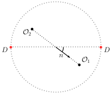
In the next section, we will be concerned with the two-point function of bulk primaries. In [26], two convenient configurations for this correlator were discussed, which we call the bulk radial frame and the defect radial frame.
Bulk radial frame.
In the bulk radial frame, the defect is a -sphere of unit radius centered in the origin. The operators are inserted in and , with
| (81) |
where is a unit vector in and . The configuration, which is depicted on the left in fig. 1, naturally defines the two cross-ratios
| (82) |
The polarization vectors are
| (83) |
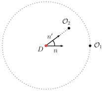
Defect radial frame.
On the other hand, in the defect radial frame the defect is taken to be flat and the operators are located at
| (84) |
where , and are now unit vectors in the transverse space , i.e. . The coordinates of can be taken as cross ratios:
| (85) |
and the configuration is depicted on the right in fig. 1. The polarization vectors are
| (86) |
4 Spinning conformal blocks
We would like to study the two-point function of symmetric and traceless bulk operators , with dimension and spin , in the presence of a defect:
| (87) |
We are going to consider the conformal partial wave decomposition of the two-point function both in the bulk and the defect channel. In the bulk channel one has
| (88) |
Here is the one-point function coefficient, which is implicit in (55) and appears explicitly in (56). The are the three-point function OPE coefficients defined in (37). The exchanged operator with conformal dimension and spin needs to have a non-vanishing one-point function in order to appear in the bulk OPE. From the discussion of subsection 3.2 we therefore conclude that all the Cartan labels of are forced to be even numbers.
The defect channel expansion is written as follows:
| (89) |
where bulk-defect OPE coefficients , were defined in (67). The exchanged operator is labelled by its conformal dimension , the representation and the representation . As explained in subsection 3.2, the parallel spin is always traceless and symmetric, while the transverse spin may be in a mixed symmetric representation .
It is often convenient to study conformal blocks in the radial coordinates defined in 3.3. Following the conventions of [26], we expand the partial waves in terms of a sum of conformal blocks, which depend on two cross ratios. In the bulk channel, from (88) we define
| (90) |
where the structures are defined in (62) and is the following function
| (91) |
A similar expansion holds for the defect channel partial waves (89), where we define as in 3.3:
| (92) |
In tables (93-94) we give some examples of conformal blocks which appear in various two-point functions of bulk operators with spin and . The notation is as follows. When the number of OPE tensor structures (which we recall are labeled by in the bulk channel and in the defect channel) is , we call the associated conformal block a seed block. The label is the number of tensor structures in the two-point function, according to (90) and (92).
| (93) |
From tables (93) and (94), we see that the total number of partial waves in the bulk and defect channels is equal. They are also equal to the number of two-point function tensor structures . For instance, the two-point function of spin one operators can be decomposed in bulk partial waves, or in defect partial waves and has . Similarly, the two-point function of spin two operators is decomposed in bulk CBs and in defect ones and again . In fact one can check that this match continues also for external operators with higher spin. It would be interesting to justify this match by using representation theory as it was done in [37] for correlation functions in CFTs without defects.
| (94) |
In the following, we describe some techniques to determine the conformal blocks and in formulae (90) and (92). In general, the bulk CBs are going to be computable only as an expansion in radial coordinates: roughly speaking the bulk CBs are as hard as the CBs for the four-point function, with which they share the same bulk OPE. On the other hand we will be able to determine a closed form formula for any defect channel CB.
4.1 Bulk channel
The bulk channel partial waves (89) are eigenfunctions of the quadratic Casimir operator:
| (95) |
The eigenvalue is and the generators are . Different partial waves associated to the same operator are distinguished by the asymptotic behavior in the OPE limit. Equation (95) can be cast into a set of second order partial differential equations which couple the functions defined in (90) for . We schematically write
| (96) |
Here the matrix depends on the cross ratios , and the derivatives . A closed form solution for generic dimension and codimension is not known.
The goal of this section is to compute spinning conformal blocks by generalizing different methods that were used in [26] to compute the scalar blocks. First, we explain how to write CBs as a series expansion in the radial coordinates. The coefficients of the expansion can be computed in various ways. In particular, we comment on an efficient way to generate them through a recurrence relation of the kind introduced by Zamolodchikov in [38]. Finally, we explain how to obtain the spinning conformal blocks by acting with differential operators on seed blocks, following the idea of [29].
4.1.1 Radial expansion
The existence of the bulk OPE implies that the bulk CBs can be written as a power expansion in the radial coordinates of section 3.3 (see [39, 40, 26]). In fact, by writing the two-point function in the cylinder frame (81), it becomes clear that the powers of measure the cylinder energy of the operators exchanged in the OPE. The dependence on the unit vector is fixed by the representations of the descendants, and encoded in the polynomials of (59). Finally, the expansion can be conveniently repackaged in a finite number of functions in one-to-one correspondence with the three-point function tensor structures given in subsection 2.3.
The object of interest is the following matrix element in radial quantization:
| (97) |
where is the projector onto the conformal family with highest weight labelled by and spin and is the Hamiltonian conjugate to the cylinder time . The function is equivalently obtained by writing the conformal partial waves into the bulk radial frame101010 In practice, the freedom contained in the coefficients is translated in the freedom of choosing the coefficients in eq. (107) below.
| (98) |
as explained in appendix C.1. In this section we define with the parallel projector for spherical defects, namely the diagonal matrix with ones followed by zeros. Eq. (98) makes it manifest that in the radial frame the functions can be expanded in tensor structures generated by the building blocks . It is natural to rewrite the projector in (97) as a sum over a complete basis of bulk states:
| (99) |
where we sum over all states at level of the conformal family, organized in irreducible representations (irreps) with spin of . labels the degeneracy of such states.
The one-point function is always fixed in terms of a single tensor structure. For example when we have
| (100) |
The case of generic is just a straightforward generalization. Equation (100) implies that the only allowed one-point functions correspond to states for which all the Cartan labels are even integers. While we pointed out in subsection 3.2 that this is true for primary operators, we now see that the same holds for descendants as well, but only when acting on the vacuum at the center of a spherical defect.
The overlaps of (99) were already considered in [40]. For concreteness we present here some examples of their form. If is a symmetric and traceless representation, the overlap is fixed by Lorentz invariance up to a few coefficients ,
|
|
(101) |
where we introduced the covariant derivative on the sphere . The coefficients multiply the tensor structures . The tensor structures are homogeneous functions of of degree and are generated as products of the following five building blocks (we take all the derivatives to be ordered on the right of the polynomial):
| (102) |
For example, for one external vector we get two structures
| (103) |
While for two external vectors we get five structures
| (104) |
The exchange of other representations require appropriate projectors in eq. (101). For instance, if the primaries and are vectors, they also exchange operators in the representation ,
| (105) |
Notice that in this case there are no tensor structures since all the polarization vectors , are being contracted with the projector. In fact this is a seed three-point function as defined in (43).
Putting all together, one obtains a general formula for the radial expansion:
| (106) | ||||
| (107) |
where .
Notice that the sums in (106) over and span a finite sets of elements: is bounded by the number of tensor structures in the OPE , while the Cartan labels are bounded by the possible representations exchanged in the OPE and need to be even. This means that to compute the conformal blocks we need to know a finite number of functions . They are constrained by Lorentz symmetry as shown in equation (107), where the only unknowns are the coefficients . Equation (107) provides a natural expansion in radial coordinates, where at each new level in there is a finite number of coefficients to be computed.
In (107) we loosely write , where are the polarization vectors of the external operators. This is a schematic formula to stress that all the complication of a mixed symmetry exchanged representation are encoded in the polynomials defined in (59). More precisely, in the definition (59) each line of the Young tableau is contracted with the same polarization vector, while in (106) different polarization vectors may appear in the same line. Let us exemplify this construction with the two-point function of vector operators,
| (108) |
where the structures are defined in (104). We dropped the label from since it only has one tensor structure and we omitted the dependence on from since it does not depend on them. The definition of the functions is as follows,
| (109) | |||||
| (110) |
The purpose of the derivative is to insert the polarization vector in the second line of the Young tableau, in accordance with equation (105).
The final task is to fix the coefficients . A possible strategy uses the Casimir equation, which can be cast as a recurrence relation for the coefficients . This strategy was used for example in [26] to compute the bulk channel scalar CBs. In the next subsection, we explain instead how to compute them using a recurrence relation akin to the one Zamolodchikov proposed for Virasoro CBs [38].
4.1.2 Zamolodchikov recurrence relation
In [26] we explained how to write a Zamolodchikov recurrence relation [38] for scalar bulk blocks following the recipe of [41, 42, 43]. Here, we show that it is easy to generalize the Zamolodchikov recurrence relation to the case of external operators with spin. Following the argument of [43], a conformal block for the exchange of an operator of conformal dimension and spin , has the following pole structure as a function of :
| (111) |
In equation (111) we denoted by and the labels of the operator which is a descendant of . The descendant operator becomes primary when we tune the dimension of the primary to , in which case , where is the level. Being both a primary and a descendant, has a vanishing norm, which in turn gives rise to a pole in the conformal block [43]. We break up the matrix into the following pieces:
| (112) |
where the coefficients and take into account the different normalization of the operator with respect to a canonically normalized operator with the same spin as [26, 43]. In particular are defined by
| (113) |
while the matrix implements the following change of basis,
| (114) |
As we explained in [26], the pole structure matches the one of the conformal blocks for theories without defects [43, 40]. However, in this case the spins are even integers, while the four-point function of local operators also exchanges odd integers [43, 40]. For completeness, we write the full set of poles and the quantum numbers of the associated primary descendants in the following table
| (115) |
where .
Also the coefficients and the matrices are the same as the ones defined in [43]. They were computed for the vector-scalar and the vector-vector cases in [43, 40, 10]. Finally, was computed in Appendix B.2 of [26] for all the operators in a symmetric and traceless representation.
The conformal blocks (90) are obtained by summing over all the poles in and the regular part as follows:
| (116) | |||
| (117) |
The functions can be computed by solving the Casimir equation at leading order for . Notice that, since , we can use this recurrence relation to compute the radial expansion of the conformal blocks.
4.1.3 Spinning differential operators
It is possible to obtain spinning conformal partial waves in the presence of defects by acting on seed conformal partial waves with appropriate differential operators , first defined in [29]. These differential operators act by effectively increasing the spin of operators in a three-point function
| (118) |
where and . The three-point function on the left hand side of (118) is a representative seed of the kind (44) (here we named ), while the one on the right hand side is a generic three-point function, thus it is labeled by a tensor structure index . The result of [29] is that can be constructed as compositions of the following elementary operators
| (119) |
and as defined in (37). With the above definitions increases the degree in and by one unit, while increases both and . With respect to [29], we want to consider an extra operator which increases the degree in while deceasing the degree of by one unit. This is the so called spin transfer operator of [32] defined in equation (201) in appendix B. This has the special role of mapping seeds in seeds (see appendix (B.1)). Therefore it allows us to construct all the seed three-point functions (43) from its action onto the seed representatives (44).
The bulk OPE is not affected by the presence of the defect. This means that it is possible to generate the spinning blocks in the bulk channel by acting with on the (representative) seed partial waves,
| (120) |
In appendix (B.1) we show that the full set of partial waves (for in traceless and symmetric representations) is obtained by acting on seed partial waves with the following combinations:
| (121) |
The label counts the choices of non-negative integers which satisfy the constraints (39). The operator implements the shift on the external dimensions .
We put a bar on the OPE label because the basis of differential operators is different from the OPE basis (labelled by ) defined in (63). There is however a linear map between the two bases which can be easily obtained acting with on the representative seed and expressing the result in terms of the OPE basis (63). This problem was already addressed in the paper [29] (see equation (3.31)). The matrix is computed explicitly in few examples in appendix B.
As in the case of a four-point function of local operators, the differential operators (121) are not sufficient to generate all the blocks, since they do not provide a way to compute the seed representatives. In the four-point function case the problem was solved by the introduction of weight shifting operators [36] which can be used to generate seed blocks by acting on scalar ones. It would be interesting to generalize this technology to defect CFTs.
Finally, it is important to stress that there are just three new seed blocks which need to be computed in the case of the two-point function of spin two operators with a defect in generic dimensions. This has to be compared with the eight (non symmetric and traceless) seeds which are needed to tackle the case of the four-point function of stress tensors. In order to compute the missing seeds (in radial expansion) one can apply the techniques explained in the sections above. Moreover, in three spacetime dimensions only traceless and symmetric representations are allowed, therefore by acting with spinning differential operators [29] on the scalar bulk channel CB one can generate the full set of bulk channel blocks.
4.2 Defect channel
In the following, we show that the full set of defect partial waves can be written in a closed form. In particular, they are simply related to the set of special functions introduced in (17). The functions explicitly computed in [32, 35] are sufficient for obtaining all the defect CBs “of interest”. In order to further illustrate and check the results, in subsections 4.2.3 and 4.2.4 we also extend the radial expansion techniques to the defect channel. A list of computed conformal blocks for external vector operators is presented in appendix F.
The factorized form of the defect symmetry group gives rise to two independent Casimir equations for the parallel and transverse factors. We claim, and check in various cases, that the conformal partial waves (92) can be written in embedding space in a completely factorized form:
| (122) |
The functions and are eigenfunctions of the parallel and transverse Casimir equations respectively (with appropriate boundary conditions), namely
| (123) |
Here is defined as where the suffix () means that we consider the indices to be in the parallel (transverse) space. The eigenvalues are
| (124) |
Notice that commutes with both the Casimir operators. This implies that the defect conformal blocks are independent of the dimensions of the external operators.
4.2.1 Seed blocks as projectors
Our strategy will be to obtain a closed form expression for the so called seed partial waves and then to act on them with differential operators in order to generate the full set of conformal blocks.
In this subsection we explain how to obtain all the seed conformal blocks in terms of the mixed symmetry projectors found in [32], schematically
| (125) |
Let us now explain the ingredients that enter formula (125). From the discussion in subsection 3.2, defect seed conformal blocks appear when the representations of the external operators satisfy the following relation:
| (126) |
where and are respectively the parallel and transverse spins of the exchanged operator . For the sake of clarity, and in line with the main focus of the paper, from now on we restrict ourselves to the case of external traceless and symmetric primaries with spin and ,
| (127) |
It is convenient to rephrase the condition (126) as a property of the parallel and transverse seed partial waves defined in (122). The factorized seeds need to satisfy the following scaling properties:
| (128) |
This implies in particular that the full seed block satisfies the seed condition (126). As we remarked at the end of section 3.2, seed blocks are automatically conserved.
We claim that all the transverse seed blocks can be simply written in terms of the polynomials (17). For example, if the external operators are symmetric and traceless we can write all the transverse seeds as follows
| (129) |
This can be easily seen from the leading defect OPE as we will describe in more detail in section 4.2.3. From an abstract point of view, one can check that (129) satisfies all the required properties to be a seed. In fact (129) has the appropriate scaling (128) and it satisfies the Casimir equation (123). In addition, (129) is conserved. All of this immediately follows from the properties of the projectors described in subsection 2.1.2.
We moreover claim that also the parallel seed blocks can be written in terms of the polynomials (17). This statement may look less trivial since the parallel seed is not a polynomial. However, if is a negative integer the parallel seed satisfies the same set of properties as the transverse one, thus, in this special case, we are lead to write
| (130) |
On the other hand, we are interested in the case where is a positive real number. We therefore define (130) as the analytic continuation of (17) for a Young tableau with a negative real number of boxes in the first row. In practice, this analytic continuation is straightforward: roughly speaking it amounts to replace a Gegenbauer polynomial by a Hypergeometric function .111111This kind of analytic continuation applied to different physical problems also appeared in [35, 44]. As an example, we first revisit the scalar case, where the projector into the traceless and symmetric representation simply reduces to the Gegenbauer polynomial (18). The transverse partial wave is in fact . The parallel one can be written as [20]
| (131) |
Notice that the parallel block is equal to the Gengenbauer when is a negative integer, up to an overall normalization. Thus, is an analytic continuation of the projector (18) for a number of boxes in the first row, and for . It is easy to check that the function has the correct asymptotic behaviour to describe a defect conformal block. We claim that even for more general Young tableaux we can still use the prescription
| (132) |
Notice that this replacement is easy to perform since every projector in [32, 35] is written in terms of an explicit differential operator acting on a single Gegenbauer polynomial as shown in (22).
Equations (129-130) are powerful formulae. Indeed, just by knowing (18) and (21) we automatically obtain the seed blocks for the exchange of the operators (which appears for scalar external operators, ), , (which appear for ) and (for ). In [35] it is explained how to obtain projectors with an arbitrary number of boxes in the second row by applying differential operators on the traceless and symmetric projector. This implies that from (129-130) we can obtain the defect seed blocks for any two point function of traceless and symmetric operators. Moreover from the projectors computed in a closed form in [32] one can also extract seed blocks for external operators in mixed symmetric representations of .
From formulae (129-130) it is also possible to argue that, when is even, the dependence on of all the seed blocks is of the form , where is a rational function of . Indeed, from formula (22), we see that all the parallel seed blocks are obtained by acting with a finite number of derivatives on the scalar block.121212To be precise, the derivatives are in the variable , but the Jacobian of the change of coordinate from to is a rational function of . Also, the schematic dependence on of formula (22) is polynomial, as one can see from the example (21). Since for even the radial part of the scalar block is of the form , we conclude that the full result takes the same form.
In the next subsection we define new differential operators of the kind explained in subsection 4.1.3 and in [29], which generate conformal blocks for external operators with generic spin by acting on a seed block. Knowledge of the seed blocks and of the differential operators allows to compute all the defect conformal blocks for external traceless and symmetric operators.
4.2.2 Spinning differential operators
In this subsection we explain how to generate all the spinning defect conformal blocks by acting with differential operators on seed blocks. First, we define a set of differential operators that create the bulk-defect spinning structures out of the seed ones. Schematically, we look for an operator such that
| (133) |
where is a generic spin and the index labels a choice of bulk-defect tensor structure as shown in (69). Following the logic explained in [29], the differential operators must be functions of positions and the polarizations of the external bulk operators . As in the bulk case, we consider to be a composition of elementary operators, each of them increasing the degree of homogeneity of of one or two units at a time. To obtain the form of the operators we first impose that their action preserves the submanifold defined by
| (134) |
While this condition was sufficient to uniquely fix the bulk differential operator, in the defect case it leaves some freedom. Therefore, we explicitly require that (133) holds, namely that the action of the differential operators on a generic bulk-defect tensor structure (67) is a linear combination of tensor structures (67). This is carefully explained in appendix E. The result is that the operator (for ) is generated by products of three elementary operators. The first two take the differential form
| (135) |
where . The third one is simply the multiplication by , defined in (53), which increases the spin by two at point .
In conclusion, we obtain a generic spinning conformal block in the defect channel just by acting with differential operators on a seed block (130), namely
| (136) |
where each operator is generated by the composition of the elementary building blocks (135) and
| (137) |
The operator implements the shift . The index labels the number of ways in which one can fix the integers such that . We introduced a barred index , since the basis (137) of the differential operators is not the same of (69) labelled by . However one can easily obtain the change of basis by performing the computation sketched in (133) and expressing the right hand side in terms of (69). This procedure gives an invertible map between the differential basis (137) and the basis (69). For more details we refer to appendix E.
The differential operators either act on the parallel space or on the transverse one. Therefore the partial waves preserve the factorized form
| (138) | |||||
| (139) |
Hence, we can write a very compact and explicit formula for all the conformal partial waves which can appear in the expansion of a two point function of any external traceless and symmetric operator:
| (140) |
Again, here the labels count the possible ways to choose and subject to the constraints mentioned above.
In appendix E we give more details on the construction of these differential operators, and provide a few examples.
One can in principle generalize this framework in order to find conformal blocks for external operators in any representation of . It would be also interesting to generalize the formalism of [36], which obtained differential operators that change the representation of the exchanged operators.
4.2.3 Radial expansion
In this subsection we show that the defect conformal blocks can be written as a convenient expansion in radial coordinates. The results presented here are a generalization of the radial expansion for scalar blocks obtained in [26] and provide a check of formula (140).
We are interested in computing the functions which are obtained by projecting the partial waves (92) onto the defect radial frame of section 3.3,
| (141) |
as detailed in appendix (C.1). We define the function by inserting a projector in the two-point function written in the defect radial frame,
| (142) |
is the Hamiltonian conjugate to the cylinder time . projects onto the conformal family with highest weight labeled by , and a Young tableau which encodes the transverse spin. With traceless and symmetric external operators, the Young tableau can have at most two rows, namely . We then rewrite the projector as a sum over a complete basis of defect states
| (143) |
where the sum over the parallel spin runs from to . Requiring Lorentz invariance fixes the general structure of the bulk-defect overlaps as follows
| (144) |
where , the indices are in parallel directions and the indices in orthogonal directions. Notice that the structures are generated by three building blocks , while the extra building block is already factorized in formula (144). The four building blocks plus the projector itself are in fact in correspondence with the embedding space structures defined in formula (69) (the projector takes into account the contributions of two structures: each column of length correspond to a while each column of length to ) . As an example, when the operator has spin and the exchanged operator has we have two possible cases: either or . When there are two possible structures,
| (145) |
On the other hand when there is just the trivial structure .
Putting together the left and right overlaps we obtain the following expression for the conformal blocks:
| (146) |
where the functions are defined as
| (147) |
with . Let us now compare the ansatz (LABEL:Ansatz_Defect_Radial_Frame) with the counterpart in embedding space (122). The transverse piece is equal to the transverse seed (129) after projecting the points to the radial frame (84). However, the full result (LABEL:Ansatz_Defect_Radial_Frame) for fixed is not factorized in a purely transverse times a purely parallel part. This is expected, since the parallel scalar products in embedding space project onto linear combinations of both parallel and orthogonal products in the defect radial frame of subsection 3.3.
At this point, the parallel functions are still unknown since the coefficients have not been fixed (in fact so far we only imposed Lorenz symmetry). In order to compute the functions it is convenient to plug the ansatz (LABEL:Ansatz_Defect_Radial_Frame-147) into the Casimir equation. This leads to simple recurrence relations for the coefficients , which we were able to solve and resum in all the cases that we considered.
In appendix C.2 we give two examples of this technique. First we consider the two point function of a vector and a scalar operator, then we study the case of two external vectors. In both cases we obtain closed form expressions for the defect channel conformal blocks which match the results of formula (140).
4.2.4 Zamolodchikov recurrence relation
In this subsection we apply Zamolodchikov’s recurrence to the defect conformal blocks for spinning external operators. Again, we focus on external operators in the traceless and symmetric representation, but everything can be easily generalized to other cases.
Spinning defect conformal partial waves have poles at special values of with residues proportional to other conformal partial waves. The expected analytic structure in the poles of a generic spinning defect conformal partial wave is
| (148) |
Note that is a matrix that mixes the various defect conformal partial waves associated to the exchange of the primary descendant operator .
We can then obtain a recurrence relation for the defect conformal blocks defined in (92) by summing over the poles in and on the regular part,
| (149) | ||||
The transverse spin is diagonal in formula (149) since is a descendant of . The sum over runs over the types (I,II,III) and the integers . When the two external operators are traceless and symmetric, the values of and can be found in the following table131313When the external operators are not in the traceless and symmetric representation there are more types which match the extra types obtained in [43].
| (150) |
and . The value of for the type III runs in general over an infinite range, while the type I and II are bounded by the spin of the external states. In fact while , where is the transverse spin of the exchanged operator. The function can be computed case by case by solving the Casimir equation at leading order in large . Finally, is defined as follows:
| (151) |
and can be computed following the same logic of [43]. In particular the ’s are obtained by comparing the normalization of the two-point function of primary descendant operators with the one of canonically normalized primaries. The expression of is the same as the one computed in [43], once we replace and and the result is reported for completeness in appendix D. The coefficients are obtained by computing the normalization of a bulk-defect two-point function where the defect operator is a primary descendant,
| (152) |
where is a canonically normalized primary with the same quantum numbers of . In appendix D we present all the ingredients to obtain the recurrence relation for the scalar-vector and the vector-vector two-point functions.
In appendix D - see equation (263) - we also show that when is even the poles of type III of any seed block have zero residue for . Thus, in this case there is a finite number of poles for any conformal block. We recover the expectation that all the defect conformal blocks drastically simplify and become rational functions of .
Let us make a general comment on the matrix in equation (151). From (152) it is easy to see that if the two point functions and do not share the same transverse tensor structures (i.e. they need to share the same in the notation of (69)). In fact the descendant is obtained by acting with parallel derivatives on , which commute with all transverse products . Thus, the block can only be proportional to for special values of and when their transverse part exactly matches. This means that just few of the (with different ) will actually be coupled in (149), or in other words that is going to be very sparse. We will explicitly see this phenomenon happening in the examples computed in appendix D.
In order to avoid the redundancy explained above it is possible to directly write a recurrence relation for any linear combination (in and ) of defined in (138), which by definition involves only the parallel part of the partial waves. We chose however to present the recurrence relation without introducing this optimization step for the sake of clarity. On the other hand, from this point of view we can give a new interpretation to the Zamolodchikov recurrence relation for defect blocks. Roughly speaking it can be understood as a recurrence relation for the (analytically continued) projectors themselves. For example the recurrence relation for the scalar CB (obtained in [26]) can be exactly interpreted as a property of when we continue into the complex plane the number of boxes in the first row of the projector. It would be interesting to expand on this point of view and see whether it may help in the construction of more generic projectors.
5 Example: the scalar Wilson line
As a further check of our formulae, we would like to apply the formalism to a specific example. We consider a theory of a complex free boson in 4d coupled to a line defect of the following form:
| (153) |
where is a straight line. is inserted in the path-integral of the free theory. The theory has a conserved current for the symmetry of the bulk:
| (154) |
while the next vector primary has dimension in :
| (155) |
In the rest of the section, we present the conformal block decomposition of correlators involving (154) and (155). We shall take to be canonically normalized: .
5.1 Decomposition of
We begin with the non-conserved vector primary (155). We choose to exhibit the two-point function rather than . Notice that the former does not vanish since the defect transforms under . After some simple Wick contractions, one finds:
| (156) |
Where the two cross ratios and are defined as [26]
| (157) |
We recall that the structures are defined as follows
| (158) |
in accordance with the discussion in section 3.
Bulk channel
The bulk OPE is constrained by charge conservation, and since has unit charge, the only contributing primaries have charge 2. Wick theorem restricts the choice to primaries built out of , with . Their one-point functions are proportional to . We learn from eq. (156) that operators with are not exchanged. As we shall see, this is enforced by the structure of the defect channel. The exchanged operators are either symmetric traceless tensors with even spin or mixed symmetric tensors with labels : this is presented in table (93), and it is easily verified using eqs. (37). Let us first consider the symmetric and traceless tensors of even spin and conformal dimensions (). It is immediate to derive the following table for the one-point functions of :
| (159) |
As it turns out, only the subset of operators with is exchanged in the correlator (156). Moreover, no representation with labels is exchanged. It can be checked that primaries in this representation exist in the spectrum of theory, with the right quantum numbers to be exchanged in the OPE of with itself.141414One can use the conformal characters [45], see e.g. [46] for the explicit computation relevant here. A direct computation for a low lying example shows that they also acquire a one-point function. The resolution is that their three-point function with the external operators vanishes. Therefore, we only compute the partial waves for symmetric traceless exchanges in appendix B, and in particular we use the basis for equal external operators defined in (213).
The decomposition reads
| (160) |
where we factored some powers of for convenience. It is interesting to notice that only the structures appear, out of the four possible.
All the exchanged operators of twist appear in the CBs decomposition weighted by coefficients which take the following form
| (161) |
We could not guess a general form for the coefficients , associated to the exchange of operators with twist . We propose a closed form result for which is compatible with the conformal block expansion up to values of ,
| (162) |
For completeness we also report the firsts few coefficients for higher twist operators (with ),
Defect channel
As summarized in table (94), this correlator can exchange defect operators in representations labeled by , or . For a line defect, is in fact only defined mod2, and measures parity under the reflection of the coordinate parallel to the defect. Again, the charge imposes selection rules. Let us promote and to background fields with the appropriate charge, so that is conserved. couples to defect operators with unit charge. Since , Wick theorem leaves four possibilities: , , , , which can be decorated by derivatives. We already disregarded operators that appear in the defect OPE of , but cannot be exchanged in the two-point function (156), e.g. operators of the form . The operator is the identity, which is not present in the defect OPE of a vector. The operators with one power of only contribute to the spectrum, since is a descendant. Furthermore, all the operators of the kind , where are indices orthogonal to the defect, are descendants up to the equations of motion. Finally, in order to anti-symmetrize the derivatives in transverse directions we need to apply them to , e.g. . All in all, we find the exchanged spectrum, and the powers of the couplings in the CFT data:
| (163) |
with except for the last line where is excluded. Let us check that this is indeed what happens.
In accordance with the discussion above, three families of defect partial waves contribute to (156), for a total of six partial waves, as presented in the Table (94). Their explicit form can be found in Appendix F. There are two defect OPE structures associated to the exchange of a spin primary with and correspondingly four defect partial waves, with . There is a unique defect OPE structure associated to the exchange of a mixed symmetric representation and therefore a unique partial wave associated to it: the seed block . Similarly, when there is a unique defect OPE structure and its associated partial wave is the seed .
The conformal block decomposition precisely obeys table (163):
| (164) | ||||
The equality of the external operators implies at the level of defect OPE structures that and similarly . In the transverse twist sector, the coefficients take the following form
| (165) |
In the even transverse twist sector (), we find
| (166) |
Finally, as expected the seed blocks only contribute to the transverse twist sector, as follows:
| (167) |
5.2 Decomposition of
Let us turn to the 2-point function of the current (154):
| (168) |
where we the structures are defined in (158) and the cross ratios in (157). As a first simple check, it is easy to verify that setting to zero the couplings , , and adjusting the normalization, one obtains the correct central charge , see e.g. [47].
Bulk channel
The fusion rule of the current involves higher twist operators. However, the bulk channel decomposition only includes, besides the identity, primaries with and (), i.e. twist two. This is enforced by crossing. As we shall point out, it is clear from the defect channel that the coupling to the defect is proportional to , and it is easy to see that only the one-point functions of operators of with twist two are compatible with the requirement. We write this decomposition in terms of the conserved blocks, presented in appendix B.3. We find
| (169) |
with coefficients
| (170) |
Defect channel
The spectrum exchanged in the defect channel can be guessed in a way analogous to the previous subsection. Part of the spectrum just coincides with the one of a trivial defect: it consists of the Taylor expansion of evaluated on the defect, and its purpose in life is to decompose the bulk channel identity [8]. The coupling to the defect happens through the operators and , which form a sector with and OPE coefficients proportional to .
Conservation reduces the number of independent OPE coefficients and, as a consequence, not all the blocks involved in the decomposition of (156) are separately consistent with the conservation in the bulk. As argued in section 4.2.1 the seed blocks and are always separately conserved and are therefore generically exchanged in the defect decomposition of (168). On the other hand, only a precise combination of blocks associated to defect primaries of transverse spin is consistent with conservation. This is denoted as and its form can be found in E.2. The decomposition in terms of the defect channel conserved blocks presented in F reads
| (171) | ||||
As anticipated, the only coefficients that depend on the couplings are those with :
| (173) |
Notice in particular the presence of a primary with : this operator is in fact protected, and required when the defect breaks a global symmetry, see e.g. [48, 18]. The coefficients are in correspondence of primaries with . We present them in closed form:
| (174) |
Finally, and receive contribution from the odd transverse twist sector ,
| (175) |
6 Conclusions
In this work, we studied correlation functions involving local operators which transform in mixed symmetry representations of . Firstly, we described a constructive procedure to obtain the tensor structures that appear in any correlation function of bosonic operators in a CFT. The procedure associates to each local operator the tensors (29). In the defect CFT scenario, the additional building blocks are the tensors (51), which take care of the quantum numbers of defect operators associated to the transverse rotations, and the projectors (45 - 46) onto the spaces parallel and transverse to the defect.
These ingredients allowed us to define explicitly all the tensor structures relevant to the conformal block decomposition of a two-point function of symmetric traceless primaries in the presence of a defect. In the second part of the paper we precisely focused on this decomposition. We explained how to generate the bulk channel conformal blocks in a radial expansion, adapting various techniques present in the literature, with special emphasis on the Zamolodchikov recurrence relation and on the differential operators first defined in [30]. For the defect channel, on the other hand, we proposed a complete solution: the seed blocks can be found in closed form performing an analytic continuation of the projectors onto representations of the orthogonal group. The generic block is then obtained by application of a set of differential operators. The structure of the radial expansion and of the Zamolodchikov recurrence relation are also explained in the defect channel, and used to check the closed form of the bocks.
With the toolbox provided here, the kinematics of a two-point function of bosonic operators with a conformal defect is tamed. Hopefully, this will be useful in all the situations in which such a correlator must be computed, whatever the technique employed.
Acknowledgments
We thank Tobias Hansen, Slava Rychkov, Petr Kravchuk, Denis Karateev and João Penedones for numerous useful discussions. We particularly thank Vasco Gonçalves for collaboration in the early stages of the project. We also thank the Simons Collaboration on the Non-perturbative Bootstrap for organizing many stimulating conferences and workshops where this work was carried out.
EL is grateful to Nikolay Bobev and Lorenzo Di Pietro for many illuminating discussions and suggestions. In addition, he thanks the Perimeter Institute for Theoretical Physics, where part of the project was carried out. Research at Perimeter Institute is supported by the Government of Canada through Industry Canada and by the Province of Ontario through the Ministry of Research & Innovation. EL is supported by the Belgian Federal Science Policy Office through the Inter-University Attraction Pole P7/37, by the COST Action MP1210, European Research Council grant no. ERC-2013-CoG 616732 HoloQosmos, as well as the FWO Odysseus grants G.001.12 and G.0.E52.14N.
MM is supported by the Simons Foundation grant 488649 (Simons collaboration on the non-perturbative bootstrap) and by the National Centre of Competence in Research SwissMAP funded by the Swiss National Science Foundation.
ET is supported by the Simons Foundation grant 488655 (Simons Collaboration on the Nonperturbative Bootstrap).
Appendix A Polynomials from projectors
This appendix is dedicated to an example of the polynomials which appear in the one-point function of primaries – equation (58) – and in the bulk channel blocks – equation (107). The polynomials may of course be constructed using the definition (59) in terms of explicit projectors, but the alternative method presented here directly yields expressions analytic in the label .
In order to obtain the polynomial in closed form, we define the following ansatz
where
and are functions of the ratio . We introduced coefficients (which could be absorbed in the definition of ) for convenience. We then require this ansatz to be compatible with the definition (59), i.e. to satisfy the properties of scaling, mixed symmetry and traceleness (5), (6), (7). These properties imply
| (176) |
where we defined
| (177) |
Note that the explicit form of this projector can be also obtained studying the analytic structure in of the bulk blocks for two external vectors (211). Indeed, as we explain in 4.1.2, the latter exhibit a I2-type pole at (which corresponds to ) with residue proportional to . This is a consistency check of our results. Notice that, since (211) are computed as differential operators acting on the scalar bulk conformal blocks, this procedure gives the projector as a combination of derivative acting on the symmetric and traceless projector .
Appendix B Spinning differential operators - bulk channel
B.1 Recurrence relation for the differential basis
Following the same logic as [29], we now derive a set of recurrence relations which allow to build generic three-point functions in terms of the action of differential operators on seed three-point functions.
The list of the relevant tensor structures was presented in equations (37) and (38). For convenience, in this appendix we denote them as follows:
| (178) |
where and the integers satisfy the condition (39). From (39) we obtain that the seed three-point functions take the form (43),
| (179) |
Notice that for a given operator (which we want to think of as the exchanged operator in the OPE), there are many possible seed three-point functions. In fact, from the conditions (41) and (43), they are labelled by the choices of and such that . Their total number is therefore . For example, if has spin there are four possible seeds which correspond to the following choices of spin for the external operators .
There exist two spin transfer differential operators , first defined in equation (D.7) of [32] and reviewed in the following subsection, which map seed three-point functions in seed three-point functions as follows,
| (188) |
| (197) |
The existence of such operators allows us to obtain all the seed three-point functions associated to a fixed operator , just by knowing one representative. This can be in turn used to compute all the seed conformal blocks for the exchanged operator just by knowing one of them. A natural choice for the representative is the three-point function , and generic .
In the following, we generalize the computation of [29] by writing the action of the differential operators (119) on the basis (178),
|
|
(198) |
|
|
(199) |
where we used from (39). Similarly we can apply the operators and which give analogous results (their action is the same as the one of and once we replace and ). Finally, of course, the multiplication by increases the label of (178) by one. As expected all the differential operators (119) act internally to the basis (178).
From the previous formulae one can easily see that acting with (119) on the set of seed three-point functions (179) it is possible to generate all the possible three-point functions. Moreover, by using the operator we can obtain all the three-point functions just by acting on the seed representative defined by and ,
| (200) |
where the integers satisfy (39) and shifts the external dimensions as . The curly bracket basis on left hand side of (200) is the differential basis defined in (121). The basis (178) and (200) are related by an invertible linear map. In appendix B.3 we explicitly compute this change of basis in few examples.
B.2 Spin transfer operators
Here we define the spin transfer operators which act by transferring one unit of spin from the operator to the operator . By this we mean that has homogeneity in and in . The spin transfer operators are defined as [32]
| (201) |
where
| (202) |
and are differential operators with weight in the variable and in the variable . They are defined as follows
| (203) | ||||
The main property of is that it acts as a derivative in while preserving the conditions . These differential operators can in fact be used to write projectors into representations labelled by Young tableaux with two rows [32].
B.3 Examples
In this section we exemplify how to use the spinning differential operators (200). We will consider simple cases in which we act on the scalar partial wave . This can be computed as an expansion in radial coordinates, as explained in [26].
Vector-scalar
We consider the case of the bulk two-point function of one vector operator and one scalar operator . In this case there are two independent conformal partial waves with associated to the exchange of the symmetric traceless operator with dimension and spin . The label is associated to the OPE tensor structures defined in (38), which we choose as follows
| (204) |
The conformal partial waves are conveniently computed using the differential operators of (121)
| (205) |
where is the scalar partial wave [26]. As we already mentioned, the partial waves are in a different basis with respect to . The two bases are related by an invertible linear map
| (206) |
The matrix is obtained performing the following computation
| (207) |
which gives
| (208) |
Vector-vector
Let us now consider the case of the two-point function of vector operators with dimensions . The two vectors exchange symmetric traceless primaries and an additional seed block – see table 93. Here we take care of the first class of operators, which have dimension and spin . There are five possible partial waves labelled by the OPE index . The index is related to the following choice of OPE tensor structures:
| (209) |
We can compute the partial waves by acting with differential operators on the scalar partial wave as shown in (121)
| (210) |
The partial waves are obtained after the following change of basis:
| (211) |
where the matrix , obtained similarly to the previous case, is
| (212) |
Identical vectors
When the external vector operators are equal, we must impose the symmetry under the exchange of in the set of structures (209), or equivalently in the differential basis (210). For the exchange of an operator with spin , only four of the five possible conformal blocks survive (for more details see for example [10]),
| (213) |
Identical conserved currents
We shall now focus on the case when the external operators are conserved currents. It is easy to see that only two combinations of the five tensor structures (209) are conserved. As a consequence, there are only two conserved bulk blocks (see for example [10]),
| (214) |
where must be even. Here the are associated to the basis (209) (of course one can rewrite this relation in the differential basis using (211)). The coefficients are defined as follows,
| (215) |
As a last remark, we mention that for only the block survives: identically vanishes.
Appendix C Conformal blocks in the radial frame
C.1 Two-point function in the radial frame
In the main text we explained that a two-point function of bulk operators can be decomposed in the tensor structures (63). In this appendix, we explain how to decompose the same two-point functions in terms of tensor structures directly in the bulk or defect radial frames. Two sets of tensor structures will naturally appear, depending on the choice of frame. We shall see that two linear maps exist, which relate the embedding space structures (63) to both the bulk and defect radial frames structures.
Bulk radial frame
The partial waves in the bulk radial frame, as defined in (98), are obtained by evaluating and as in (81) and (83). In the bulk radial frame it is convenient to expand the two-point function in terms of a set of tensor structures ,
| (216) |
The coefficient of each tensor structure is a function of the radial coordinates. The index runs over a finite range which depends on the choice of the two external operators. The tensor structures are polynomials in the eight variables
| (217) |
The have degree in each polarization . For instance, for one external vector the decomposition (216) takes the form
| (218) |
Notice that the first four structures in (217) have weight 1 either in or in and the last three have weight (two of them in the same and two of them in both and ). The number of building blocks and their weights match the embedding space definitions (60). In fact, there is a map between the building blocks (60) and (217), which is obtained by projecting (60) onto the bulk radial frame. For instance,
| (219) |
It is important to notice that with the definitions (60 - 61), the small limit of the tensor structures is regular and non-degenerate,
| (220) |
Therefore there exists a linear map between the structures and of (63), which is invertible also in the leading bulk OPE limit (when ).
Defect radial frame
Similarly, one can define the two-point function in the defect radial frame (141) via equations (84) and (86). Therefore, we can expand in a basis of tensor structures
| (221) |
As in the bulk case, the tensor structures are generated by building blocks:
| (222) |
For instance, for one external vector we have
| (223) |
Again, we can map the building blocks (222) to the ones defined in (60) by projecting the latter onto the defect radial frame. For instance,
| (224) |
C.2 Examples - defect channel
Here we present two explicit examples of application of the Casimir recurrence relation, mentioned in subsection 4.2.3, to the computation of defect channel conformal blocks.
Vector-scalar
Consider the two-point function of a vector and a scalar . The tensor structures are written in (145). We therefore get that formula (LABEL:Ansatz_Defect_Radial_Frame) reduces to
| (226) |
where we dropped the index , since it can only take the value . The function is written in terms of a Gegenbauer polynomial as follows
| (227) |
Using the identity
| (228) |
where is a generic function, we can rewrite (226) in the basis of the two structures and to match (223),
| (229) |
The basis of and can be mapped to the usual and basis by a linear transformation. It is therefore trivial to write the Casimir equation as a differential equation for the functions . The transverse part of the Casimir is solved by the ansatz (229). On the other hand, the parallel part of the Casimir acts on the functions and implies recurrence relations for the coefficients . Notice that using this basis of functions the recurrence relations decouple. For we get
| (230) |
while for we get the same recurrence relation of the scalar conformal block [26] and therefore the solution is
| (231) |
The recurrence relation for in slightly more involved and it can be solved to find
| (232) |
in terms of the initial condition . It is then straightforward to resum the series in obtaining
| (233) | ||||
The coefficients set the normalization of the conformal blocks. They can be fixed to reproduce the defect OPE limit.
Vector-vector
We repeat the previous exercise for two external vectors. In this case can be either or . When we have the structures (145) for both the left and the right overlaps (of course for the right overlap we need to replace and ). When there is a unique structure given by . If the exchanged operator is in a traceless and symmetric representation of , the decomposition (216) becomes
| (234) | |||||
where we dropped the indices of since there is a single tensor structure in this case. We remind that the transverse part of these functions is already solved by the ansatz (234), we only need to find and . To do so we make use of the parallel Casimir equation.
In this case, according to formula (63), the tensor structures in the bulk two-point function are six, matching the six radial frame structures:
| (235) |
The Casimir equation gives a set of six coupled differential equations which simplify using the ansatz (234). Firstly, we obtain that one of the equations can be dropped, since it is linearly dependent from the other ones (there are six differential equations for five functions). Secondly, three of the five remaining equations can be decoupled, so that only and are still coupled. Finally, the resulting set of equations can be solved exactly for the five functions. In particular, when there are only four linearly independent conformal blocks labelled by the constants (for ) which parametrize the leading behaviour of for according to (147),
| (239) |
where
| (240) |
The extra constant , associated to the leading behaviour , does not appear since it is forced to vanish by consistency with the Casimir equation. Similarly when the Casimir equation forces , therefore we obtain a single conformal block labeled by the constant ,
and all the other functions vanish.
Appendix D Zamolodchikov recurrence relation - defect channel
In this appendix, we show explicit examples of the Zamolodchikov recurrence relation for the defect conformal blocks explained in section 4.1.2. We only focus on the case of external operators in a traceless and symmetric representation, but the generalization to more complicated representations can be obtained following [43].
Before we go to the examples, let us stress that most of the results presented in [43] and reviewed in [26] still apply to the defect case. In particular it is convenient to define defect primary states as
| (242) |
where the orthogonal indices are left implicit. We then define the following descendant states
| (243) |
with and types with . The operators are the same of [43] after we replace , and the scalar product with the parallel one (for a flat defect)
| (244) |
where is the generator of translations and
| (245) |
The descendant states in (243) become primaries when with
| (246) |
Finally, the inverse norm of the primary descendants have residues predicted by
| (247) | ||||
The states also transform under transverse rotations, but the latter commute with the conformal transformations on the defect. Hence, the operator in (243) is diagonal in the transverse spin , and consequently so is the recurrence relation (149).
D.1 Examples
Vector-scalar
We consider the two-point function of a vector and a scalar . As we showed in table (94), in this case there are two partial waves and which are both associated to the exchange of an operator labelled by the conformal dimension and the transverse spin (the only allowed parallel spin is , so we will drop this label). We associate the label of to the tensor structures defined in (67)
| (248) |
We also expand each partial wave in conformal blocks as defined in (92). The label is associated to the choice of two-point function tensor structures defined in (62),
| (249) |
From table (150) we see that the only type of poles which is allowed is the type III (this is in fact the only type that does not change the parallel spin of the blocks at the residue). Formula (149) therefore reduces to
| (250) | ||||
where and . To compute the matrix we use the prescription of formula (151). The coefficient was defined in the beginning of this appendix, while is the same as the ones of the scalar blocks. To compute we follow the recipe (152). We write the two bulk-defect tensor structures (248) in the Poincaré section
| (251) |
Here, without loss of generality, we placed the bulk primary at the origin in the parallel space, so that only has transverse components.
We then use the definition (243) of the primary descendants to obtain the following equation which defines the matrix ,
| (252) |
Here, the differential operator reduces to because . The result is
| (253) |
As mentioned in subsection 4.2.4, the matrices are expected to be very sparse since we can only couple conformal blocks which have exactly the same orthogonal part. In the present case the two OPE tensor structures (248) cannot couple since they have a different orthogonal structures, namely . We conclude that the recurrence relations (250) for are decoupled.
From the Casimir equation of the defect channel, it is easy to compute the large limit of the conformal blocks. The boundary conditions are provided by the defect OPE limit . The result is
| (254) |
where is defined in (227) and . We conclude that , thus (250) becomes a simple set of two decoupled recurrence relation for and . One can use (250) to compute the conformal blocks efficiently in a radial expansion. However a closed form solution for such blocks exist, as we show for example in (271).
Vector-vector
We now study the bulk two-point function of two vectors and . As shown in table (94) this case is more involved, since there are six different partial waves for the exchange of operators in three possible representations labelled by , the parallel spin and the transverse spin . For there are four partial waves, with , labelled by the same choice of OPE tensor structures as defined in (248). When there is a single OPE tensor structure available, , which gives rise to the seed block . Finally we can build another seed block when the exchanged operator is in the mixed symmetric representation of the transverse spin. This case is completely decoupled from the previous ones since the exchanged operator lives in a different transverse representation, therefore we will consider it separately in the end of this section.
Using (92) we write the six partial waves in terms of conformal blocks . The index is associated to the tensor structure defined in formula (158). From table (150) we see that in this case, beside infinitely many poles of type III, there are two new allowed poles: the for and the for . Equation (149) can be therefore written as the following set of recurrence relations
| (255) | ||||
The coefficients are obtained using equal to the matrix computed in (253). The coefficient is fixed in terms of
| (256) |
In the recurrence relation for the residue of the type III can be computed as , where
| (257) |
Finally the matrix is obtained from
| (258) |
Since the second component in (256) and (258) vanishes, we find that is the only conformal block that couples to . This fact has a simple explanation: and are the only partial waves with the same orthogonal part in the OPE tensor structure, namely . Moreover, since (253) is diagonal we obtain that all the in (255) are decoupled from each other. The pole structure of formula (255) is now explained.
The last missing ingredient is the large delta behaviour of the conformal blocks. Solving the Casimir equation at large with initial conditions fixed by the leading OPE we find
| (259) |
where all the other functions are zero. We thus find that for most the functions (255) are strictly zero.
We can now move to the partial wave . This is actually a trivial case, since the associated function has the same recurrence relation as the scalar defect block. Indeed, all the dependence on the external spin is absorbed in the transverse piece of the partial wave. The only difference is the large behaviour, which has to be replaced by
Seed blocks
In this paragraph, we show that all the seed blocks in even dimensions have a finite number of poles in . To see this, it is sufficient to check that only a finite number of poles of type III contribute to the Zamolodchikov expansion (149), since type I and II poles are always finitely many (see the comment to table (150)).
We focus on the case of external operators in a traceless and symmetric representation of spin . A seed partial wave appears when where and are respectively the parallel and transverse spin of the exchanged operator . In this case the partial wave has a unique OPE tensor structure proportional to (times the transverse part), which in the Poincaré section gives
| (261) |
In equation (261), the position vector only has transverse components. We omitted the transverse tensor structures since they are unimportant for this argument. One can easily check that
| (262) |
for any and . The coefficient reads
| (263) |
When the dimension of the defect is an even number, the right hand side of (263) vanishes for all (beside the case , where the zero is at ). Therefore, for even , any defect seed block has a finite number of poles in in the recurrence relation (149). This is a clear indication of the simplicity of the defect conformal blocks in even dimensions, which we expect to reduce to rational functions of multiplied by as explained in section 4.2.1.
Appendix E Spinning differential operators - defect channel
E.1 Recurrence relation
In this appendix, we check that the differential operators (137) are correct and can be used to generate all the bulk-defect tensor structures of (and consequently all the conformal blocks). We consider defect operators with traceless and symmetric parallel spin and transverse spin . The bulk operator has conformal dimension and traceless and symmetric spin .
The list of the relevant tensor structures was presented in equations (67) and (69). In this appendix we will denote them as follows
| (264) |
We remind that the integers and need to satisfy the condition (70) which depends on , and . The form of the operators can be fixed as in (135) by requiring that their action closes on the span of (264). In other words, we require their action on any of the (264) to be expressed as a linear combination of the (264). Using (135), we explicitly find
| (265) |
From these equations it is clear that one can use the spinning operators to generate recursively all the building blocks (264), if one knows all the bulk-defect seeds
| (266) |
Notice that in the seeds (266) the bulk and the defect operators have the same spin , as required by (70). For example, the scalar conformal block (269) is associated to the bulk-defect seed .
E.2 Examples
In this subsection we exemplify how to compute defect channel blocks by acting with the spinning differential operators (137) on seed blocks. We will focus on simple examples for which there is a unique seed: the scalar one. In the following we denote its partial wave as
| (268) |
where the exchanged operator , has conformal dimension , parallel spin and transverse spin . The associated conformal block is [26, 20]
| (269) |
where is defined in (227).
Vector-scalar
In the case of one external vector (say the first operator), we have two independent conformal partial waves , associated to the exchange of defect primaries. These can be obtained from the scalar conformal partial wave (268) as follows
| (270) |
where the normalization is fixed to recover blocks in the OPE basis (264). Each of the can be decomposed as in (92) with given by (249). We find
| (271) | ||||
where is defined in (269).
Vector-vector
There are six independent bulk-to-defect conformal partial waves associated to the exchange of a defect primary . The four of them with (and arbitrary transverse spin ) can be obtained by applying (137) to the scalar conformal partial wave as follows
| (272) |
where we fixed the normalization consistently with (264). The remaining two conformal partial waves are seeds and are obtained by different methods (see the appendix E.1 and subsection 4.2.1). Their explicit expression is reported in appendix F.
Two currents
As reported in the third line of table (94), there is a total of six conformal partial waves in the defect OPE of a two-point function of vector operators. In the following we shall consider the case of the two-point function of conserved currents (which have protected dimension and satisfy the conservation equation ).
In order to understand the constraint of conservation it is convenient to classify the possible bulk-defect tensor structures (67). When the defect operator has parallel spin and transverse spin there are two independent tensor structures.
| (273) |
It is easy to see that the expression (273) only satisfies conservation when the OPE coefficients are related as follows
| (274) |
When the coefficient is absent and conservation implies that the correlation function vanishes, unless .151515The presence of such a defect operator denotes the breaking of the global symmetry associated to the conserved current by the defect, see e.g. [48, 18]. The conserved structure corresponding to (274) can be generated also in the differential basis (267)
| (275) |
Therefore, (275) can be used to build the single conserved block as follows
| (276) |
As we have shown in table (94), we can also build the two seed conformal blocks and . Since they are seed blocks, they are automatically conserved, as we argued in subsection 4.2.1. As a check of this statement one can consider the bulk-defect structure associated to the block ,
| (277) |
It is easy to see that (277) is conserved. Ultimately, this is a trivial consequence of the fact that the operator is a scalar primary, which cannot couple to a defect primary with .
In sum, when the external operators are two conserved currents, there is a total of three conformal blocks: , and .
Appendix F The explicit vector-vector blocks in the defect channel
In this appendix we collect the results for the defect blocks for external vector operators, which are relevant to the examples presented in section 5. These blocks are computed in a closed form with various techniques. In subsection 4.2.1 it is explained how to obtain all the seed blocks as projectors and how to get the most generic block by acting on a seed with differential operators (as exemplified in appendix E.2). In appendix C.2 it is shown how to obtain the same blocks by directly solving the Casimir equation taking advantage of a suitable ansatz. Finally, in appendix D.1 an explicit recurrence relation for the radial expansion of the blocks was derived (in this case however the resummation of the series was not attempted). All the techniques give the same result.
Even if the blocks are already written in three different ways throughout the paper we decided, for the sake of clarity, to report them here in their most transparent form, as function of the cross ratios which multiply the basis of bulk-bulk tensor structures, following the definition (92). In particular, for two external vectors, a conformal partial wave is fixed in terms of five functions () which multiply the basis of defined in (158). The blocks associated to the exchange of a defect primary with spin can be computed for example using (272),
| (278) |
where is defined in (269). The seed block associated to the exchange of a defect primary with mixed symmetry has only and components in the basis (158):
| (279) |
where we introduced the auxiliary function
| (280) |
The seed block associated to the exchange of a defect primary with symmetric and traceless transverse spin has only and components in the basis (158):
| (281) |
References
- [1] J. L. Cardy, “Conformal Invariance and Surface Critical Behavior,” Nucl.Phys. B240 (1984) 514–532.
- [2] P. Liendo, L. Rastelli, and B. C. van Rees, “The Bootstrap Program for Boundary CFTd,” JHEP 07 (2013) 113, arXiv:1210.4258 [hep-th].
- [3] D. Gaiotto, D. Mazac, and M. F. Paulos, “Bootstrapping the 3d Ising twist defect,” JHEP 1403 (2014) 100, arXiv:1310.5078 [hep-th].
- [4] F. Gliozzi, P. Liendo, M. Meineri, and A. Rago, “Boundary and Interface CFTs from the Conformal Bootstrap,” JHEP 05 (2015) 036, arXiv:1502.07217 [hep-th].
- [5] F. Gliozzi, “Truncatable bootstrap equations in algebraic form and critical surface exponents,” JHEP 10 (2016) 037, arXiv:1605.04175 [hep-th].
- [6] P. Liendo, C. Meneghelli, and V. Mitev, “Bootstrapping the half-BPS line defect,” arXiv:1806.01862 [hep-th].
- [7] M. Hogervorst, “Crossing Kernels for Boundary and Crosscap CFTs,” arXiv:1703.08159 [hep-th].
- [8] M. Lemos, P. Liendo, M. Meineri, and S. Sarkar, “Universality at large transverse spin in defect CFT,” arXiv:1712.08185 [hep-th].
- [9] D. Poland, S. Rychkov, and A. Vichi, “The Conformal Bootstrap: Numerical Techniques and Applications,” arXiv:1805.04405 [hep-th].
- [10] A. Dymarsky, J. Penedones, E. Trevisani, and A. Vichi, “Charting the space of 3D CFTs with a continuous global symmetry,” arXiv:1705.04278 [hep-th].
- [11] A. Dymarsky, “On the four-point function of the stress-energy tensors in a CFT,” JHEP 10 (2015) 075, arXiv:1311.4546 [hep-th].
- [12] A. Dymarsky, F. Kos, P. Kravchuk, D. Poland, and D. Simmons-Duffin, “The 3d Stress-Tensor Bootstrap,” JHEP 02 (2018) 164, arXiv:1708.05718 [hep-th].
- [13] S. Balakrishnan, T. Faulkner, Z. U. Khandker, and H. Wang, “A General Proof of the Quantum Null Energy Condition,” arXiv:1706.09432 [hep-th].
- [14] L.-Y. Hung, R. C. Myers, and M. Smolkin, “Twist operators in higher dimensions,” JHEP 10 (2014) 178, arXiv:1407.6429 [hep-th].
- [15] L. Bianchi, M. Meineri, R. C. Myers, and M. Smolkin, “Rényi entropy and conformal defects,” JHEP 07 (2016) 076, arXiv:1511.06713 [hep-th].
- [16] A. Lewkowycz and J. Maldacena, “Exact results for the entanglement entropy and the energy radiated by a quark,” JHEP 05 (2014) 025, arXiv:1312.5682 [hep-th].
- [17] B. Fiol, E. Gerchkovitz, and Z. Komargodski, “Exact Bremsstrahlung Function in Superconformal Field Theories,” Phys. Rev. Lett. 116 no. 8, (2016) 081601, arXiv:1510.01332 [hep-th].
- [18] L. Bianchi, M. Lemos, and M. Meineri, “Line defects and radiation in theories,” arXiv:1805.04111 [hep-th].
- [19] D. M. McAvity and H. Osborn, “Conformal field theories near a boundary in general dimensions,” Nucl. Phys. B455 (1995) 522–576, arXiv:cond-mat/9505127 [cond-mat].
- [20] M. Billò, V. Gonçalves, E. Lauria, and M. Meineri, “Defects in conformal field theory,” JHEP 04 (2016) 091, arXiv:1601.02883 [hep-th].
- [21] S. Guha and B. Nagaraj, “Correlators of Mixed Symmetry Operators in Defect CFTs,” arXiv:1805.12341 [hep-th].
- [22] M. Fukuda, N. Kobayashi, and T. Nishioka, “Operator product expansion for conformal defects,” JHEP 01 (2018) 013, arXiv:1710.11165 [hep-th].
- [23] P. Liendo and C. Meneghelli, “Bootstrap equations for = 4 SYM with defects,” JHEP 01 (2017) 122, arXiv:1608.05126 [hep-th].
- [24] L. Rastelli and X. Zhou, “The Mellin Formalism for Boundary CFTd,” JHEP 10 (2017) 146, arXiv:1705.05362 [hep-th].
- [25] V. Goncalves and G. Itsios, “A note on defect Mellin amplitudes,” arXiv:1803.06721 [hep-th].
- [26] E. Lauria, M. Meineri, and E. Trevisani, “Radial coordinates for defect CFTs,” arXiv:1712.07668 [hep-th].
- [27] M. Isachenkov, P. Liendo, Y. Linke, and V. Schomerus, “Calogero-Sutherland Approach to Defect Blocks,” arXiv:1806.09703 [hep-th].
- [28] A. Gadde, “Conformal constraints on defects,” arXiv:1602.06354 [hep-th].
- [29] M. S. Costa, J. Penedones, D. Poland, and S. Rychkov, “Spinning Conformal Blocks,” JHEP 11 (2011) 154, arXiv:1109.6321 [hep-th].
- [30] M. S. Costa, J. Penedones, D. Poland, and S. Rychkov, “Spinning Conformal Correlators,” JHEP 1111 (2011) 071, arXiv:1107.3554 [hep-th].
- [31] M. S. Costa and T. Hansen, “Conformal correlators of mixed-symmetry tensors,” JHEP 02 (2015) 151, arXiv:1411.7351 [hep-th].
- [32] M. S. Costa, T. Hansen, J. Penedones, and E. Trevisani, “Projectors and seed conformal blocks for traceless mixed-symmetry tensors,” JHEP 07 (2016) 018, arXiv:1603.05551 [hep-th].
- [33] V. K. Dobrev, V. B. Petkova, S. G. Petrova, and I. T. Todorov, “Dynamical derivation of vacuum operator-product expansion in euclidean conformal quantum field theory,” Phys. Rev. D 13 (Feb, 1976) 887–912. https://link.aps.org/doi/10.1103/PhysRevD.13.887.
- [34] F. Rejon-Barrera and D. Robbins, “Scalar-Vector Bootstrap,” JHEP 01 (2016) 139, arXiv:1508.02676 [hep-th].
- [35] M. S. Costa and T. Hansen, “AdS Weight Shifting Operators,” arXiv:1805.01492 [hep-th].
- [36] D. Karateev, P. Kravchuk, and D. Simmons-Duffin, “Weight Shifting Operators and Conformal Blocks,” arXiv:1706.07813 [hep-th].
- [37] P. Kravchuk and D. Simmons-Duffin, “Counting Conformal Correlators,” arXiv:1612.08987 [hep-th].
- [38] A. B. Zamolodchikov, “CONFORMAL SYMMETRY IN TWO-DIMENSIONS: AN EXPLICIT RECURRENCE FORMULA FOR THE CONFORMAL PARTIAL WAVE AMPLITUDE,” Commun. Math. Phys. 96 (1984) 419–422.
- [39] M. Hogervorst and S. Rychkov, “Radial Coordinates for Conformal Blocks,” Phys. Rev. D87 (2013) 106004, arXiv:1303.1111 [hep-th].
- [40] M. S. Costa, T. Hansen, J. Penedones, and E. Trevisani, “Radial expansion for spinning conformal blocks,” JHEP 07 (2016) 057, arXiv:1603.05552 [hep-th].
- [41] F. Kos, D. Poland, and D. Simmons-Duffin, “Bootstrapping Mixed Correlators in the 3D Ising Model,” JHEP 11 (2014) 109, arXiv:1406.4858 [hep-th].
- [42] F. Kos, D. Poland, and D. Simmons-Duffin, “Bootstrapping the vector models,” JHEP 06 (2014) 091, arXiv:1307.6856 [hep-th].
- [43] J. Penedones, E. Trevisani, and M. Yamazaki, “Recursion Relations for Conformal Blocks,” arXiv:1509.00428 [hep-th].
- [44] P. Kravchuk and D. Simmons-Duffin, “Light-ray operators in conformal field theory,” arXiv:1805.00098 [hep-th].
- [45] F. A. Dolan, “Character formulae and partition functions in higher dimensional conformal field theory,” J. Math. Phys. 47 (2006) 062303, arXiv:hep-th/0508031 [hep-th].
- [46] R. de Mello Koch, P. Rabambi, R. Rabe, and S. Ramgoolam, “Counting and construction of holomorphic primary fields in free CFT4 from rings of functions on Calabi-Yau orbifolds,” JHEP 08 (2017) 077, arXiv:1705.06702 [hep-th].
- [47] H. Osborn and A. C. Petkou, “Implications of conformal invariance in field theories for general dimensions,” Annals Phys. 231 (1994) 311–362, arXiv:hep-th/9307010 [hep-th].
- [48] L. Bianchi, M. Preti, and E. Vescovi, “Exact Bremsstrahlung functions in ABJM theory,” arXiv:1802.07726 [hep-th].