Mean field and beyond description of nuclear structure with the Gogny force: A review

Abstract

Nowadays, the Gogny force is a referent in the theoretical description of nuclear structure phenomena. Its phenomenological character manifests in a simple analytical form that allows for implementations of techniques both at the mean field and beyond all over the nuclide chart. Over the years, multiple applications of the standard many-body techniques in an assorted set of nuclear structure applications have produced results which are in a rather good agreement with experimental data. The agreement allows for a simple interpretation of those intriguing phenomena in simple terms and gives confidence on the predictability of the interaction. The present status on the implementation of different many body techniques with the Gogny force is reviewed with a special emphasis on symmetry restoration and large amplitude collective motion.

1 Introduction

The Gogny force, named after the renowned French physicist Daniel Gogny [1], has been used to describe many different facets of nuclear structure since its inception back in the early seventies of the past century. It has been mainly used in a mean field framework including pairing correlations where the Hartree Fock Bogoliubov (HFB) mean field is the basic entity used to obtain the quantities appearing in the theory. In this category we include not only the calculation of potential energy surfaces (PES) using constraints on the relevant collective degrees of freedom so useful to describe the shape of the ground state or the path to fission, but also extensions like the collective Schrödinger equation (CSE), the Bohr Hamiltonian approach focused on quadrupole degrees for freedom and their coupling to rotations, the QRPA or the Interacting Boson Model (IBM) with parameters determined by HFB PES. As it stands, the mean field only provides wave functions in the intrinsic frame of reference where the mean field wave function is allowed to break symmetries of the Hamiltonian. In order to compute physical observables like mean values or transition probabilities it is very important to use wave functions in the laboratory frame which have the quantum numbers of the symmetries preserved by the nuclear interaction. Therefore, in addition to the mean field, mechanisms to restore the spontaneously broken symmetries have to be applied to perform the passage from the intrinsic to the laboratory frame. These mechanisms require the evaluation of overlaps between different HFB wave function that are subsequently used in integrals over the symmetry groups. This is referred to as ”symmetry restoration” and its implementation with the Gogny force has been an active field of research since its first implementation in the early nineties. These ideas can also be used to deal with large amplitude collective motion in the spirit of the Generator Coordinate Method (GCM) often in combination with symmetry restoration. The purpose of this review is to describe the status of the implementation of all these techniques with the Gogny force putting special emphasis in those aspects related to symmetry restoration and large amplitude collective motion. There are already two long papers in the literature that overview some aspects of the applications of the Gogny force in nuclear structure but in our opinion they only offer partial views of the whole picture. In Ref [2] the authors review applications of the mean field, the 5D Collective Hamiltonian and the QRPA with the Gogny force. However, the coverage of the mean field is rather limited and fails to account for important applications like the study of high spin physics, finite temperature HFB or the applications to odd mass nuclei and multi-quasiparticle excitations as in the physics of high-K isomers. On the other hand, the review of [3] focuses only on aspects of symmetry restoration and large amplitude motion, not paying much attention to other applications beyond the mean field. Also the formal difficulties encountered in the implementation of symmetry restoration techniques with density dependent forces are scarcely discussed and also relevant technical details are overlooked. In our review we have tried to give a complete, albeit not very deep, description of all different techniques used in nuclear structure paying some attention to some relevant technical details like evaluation of matrix elements, Pfaffian techniques to evaluate overlaps or computer code implementations. Although not belonging to the family of Gogny forces we have decided to include the description of translational invariance restoration with the Brink-Boecker interaction as an illustration of this important, and often overlooked, aspect of symmetry restoration. The present review and the one of [2] can be considered as complementary as we do not cover in too much details the subjects treated by Peru and Martini.

The theoretical description of nuclear reactions with the Gogny force is not described in this review. In the last years and with the help of increasing computing power, more and more of the nuclear structure microscopic input required for reactions can be obtained from sound theoretical models with the Gogny force [4, 5, 6]. All these models are described in this review but their connection with reaction theory is scarcely discussed in the text.

The review focuses almost exclusively on applications with the Gogny force. The many body techniques used to describe nuclear structure have also been used with other interactions/functionals like the non-relativistic family of Skyrme energy density functionals or the relativistic models with great success. Although those calculations are similar and in many cases complementary to the ones presented here we are not going to discuss them and we refer the interested reader to the vast literature already available in the form of reviews.

The review is divided in six sections including the Introduction, the second section is devoted to the description of the different parametrizations of the Gogny force and several recent improvements/departures from it. In Section 3 the mean field method, adapted to deal with density dependent interactions is discussed and several examples of application with the Gogny force are presented. In Section 4 two methods beyond the mean field but not requiring Hamiltonian overlaps are described: namely the QRPA and the IBM mapping procedure. In Section 5, the issue of symmetry restoration is discussed in general and later applications to the most common types of symmetry restoration (parity, particle number projection, angular momentum projection, linear momentum projection) are presented along with several applications with the Gogny force. The difficulties encountered in the application of the symmetry restoration techniques to the case of phenomenological density dependent interactions is also addressed. Finally, in Section 6 the standard method to deal with large amplitude collective motion is discussed. Among the applications, we discuss the application of the method with symmetry restored wave functions as well as the mixing of multi particle-hole excitations intimately connected with the Configuration Interaction method. Also approximate methods based on the Gaussian overlap approximation are discussed. We conclude with a summary and perspectives section. Several appendixes with a more technical information are also included.

2 The Gogny force: its origins, motivation and present implementations

In this section a historical overview of the origins and motivation of the Gogny force is presented with special emphasis in the fitting protocols used in each of the different main parametrizations considered (D1, D1’, D1S, D1N, D1M). A few paragraphs will also be devoted to the newly proposed D2 Gogny force with a finite range density dependent interaction. Finally, we also discuss less known parametrizations including some specific terms and some forces inspired by the Gogny interaction.

2.1 The Gogny force: guiding principles

The Gogny force was conceived in a period of time when the Skyrme interaction had started to become fashionable mostly because of its ability to describe nuclear properties at the simple Hartree Fock (HF) mean field level [7, 8]. At that time, the fact that in Skyrme forces different interactions had to be used in the pairing and particle-hole (ph) channel was considered as a drawback. Also the necessity to consider a window around the Fermi level where the pairing interaction was active, was often considered as an annoying characteristic. In order to have a pairing force derived from the same central potential than the particle-hole (ph) channel, a finite range interaction, with its natural ultraviolet cutoff, had to be implemented. This is the main reason why the Gogny force was created: it had a finite range central potential that could also be used to obtain the pairing interaction. The central potential was inspired by early attempts by Brink and Boecker [9] to derive a finite range central potential with a Gaussian form for nuclear structure calculations. Going finite range was a technical challenge for the computers available at that time. However, combining together the simplicity of Gaussian shape for the central potential and a nice property of the harmonic oscillator wave functions [10], to be discussed below, gave the opportunity to get a reasonable implementation of the HF or the Hartree Fock Bogoliubov (HFB) mean fields on those days computers [11].

The Gogny force consists of four terms

$$v(1,2)=v_{c}(1,2)+v_{\mathrm{LS}}(1,2)+v_{\mathrm{DD}}(1,2)+v_{\mathrm{Coul}}(1,2)$$ (1)

A central term $v_{c}$ of finite range which is a linear combination of two Gaussians and contains the typical spin and isospin channels with the Wigner (W), Barlett (B), Heisenberg (H) and Majorana (M) terms

$$v_{c}(1,2)=\sum_{i=1,2}e^{-\frac{|\vec{r}_{1}-\vec{r}_{2}|^{2}}{\mu_{i}^{2}}}\left(W_{i}+B_{i}P_{\sigma}-H_{i}P_{\tau}-M_{i}P_{\sigma}P_{\tau}\right).$$ (2)

A two body spin orbit for zero range is taken directly from the Skyrme functional

$$v_{\mathrm{LS}}(1,2)=iW_{\mathrm{LS}}(\vec{\nabla}_{12}\delta(\vec{r}_{1}-\vec{r}_{2})\wedge\vec{\nabla}_{12})(\vec{\sigma}_{1}+\vec{\sigma}_{2}),$$ (3)

a pure phenomenological density dependent term, strongly repulsive, introduced to make the force fulfill the saturation property of the nuclear interaction

$$v_{\mathrm{DD}}(1,2)=t_{3}(1+P_{\sigma}x_{0})\delta(\vec{r}_{1}-\vec{r}_{2})\rho^{\alpha}((\vec{r}_{1}+\vec{r}_{2})/2).$$ (4)

This “state dependent” part of the interaction has to be handled properly in the application of the variational principle which is behind the HF or HFB procedures and gives rise to a so-called rearrangement potential to be discussed below. Finally, the standard Coulomb potential $v_{\mathrm{Coul}}(1,2)$ between protons is added to the interaction. Usually, the Coulomb potential is taken only into account in the direct channel of the HF or HFB procedures. The exchange term, which is rather involved due to the infinite range of the interaction, is considered in the local Slater approximation [12, 13] that comes in the form of an additional term to be added to the energy

$$E_{\rm Slater}=-\frac{3}{4}e^{2}\left(\frac{3}{\pi}\right)^{1/3}\int d^{3}\;\vec{r}\left[\rho^{P}(\vec{r})\right]^{4/3}$$ (5)

and depending on the proton’s density alone. This term also gives a ”rearrangement” contribution to the HF or HFB potentials when treated appropriately in the application of the variational principle.

The traditional center of mass correction to the mean field energy, including both the one body and two body components, is fully considered in all Gogny parametrizations and included in the variational procedure. Both the contributions to the HF and pairing (anti-pairing) fields is taken into account.

The Gogny interaction depends on 15 adjustable parameters that are obtained after performing a fit to experimental data and nuclear matter properties. Different parametrizations have been obtained throughout the years depending on the set of data and the quality of the approaches used to solve the nuclear many body problem. For a recent discussion of the fitting protocol see Ref. [14].

In the recent literature it is common to catalog the Gogny force as an Energy density functional (EDF) due to its density dependent term. In this review we will use indistinctly the term force, interaction and EDF to refer to the Gogny force.

As mentioned before, one of the main assets of the Gogny force is the use of the same central interaction both for the Hartree Fock (particle-hole) and the pairing (particle-particle)part of the HFB procedure. This property, however, is questioned by several authors using several arguments (see, for instance Ref [15]). The first argument has to do with the fact that the bare nucleon-nucleon interaction can be used in the pairing channel whereas for the p-h part a regularization of the repulsive core in the spirit of the Brueckner method is required. As a consequence, both the effective p-p and p-h channels of the interaction to be used at the mean field can be considered as unrelated and the consistency between the two channels is not required. The second argument is related to the modern view of the nuclear interactions as tools to generate energy density functionals (EDF) in the spirit of the EDF in condensed matter physics. In the nuclear physics case, those functionals must also include a pairing part that can be taken, in the spirit of the EDF, as completely uncorrelated from the rest of the EDF as long as it is able to grasp all the relevant correlations. These two arguments are mostly invoked by practitioners of the relativistic mean field and also in the non-relativistic case when zero range forces (Skyrme like) are used. It this way the use of a different interaction in the pairing channel is justified and therefore the use of the same interaction in the Gogny force can be considered more as a limitation than as an advantage. Usually a phenomenological density dependent zero range force is used in the pairing channels, although in some cases, see below, the central part of the Gogny force is used for the p-p channel. On the other hand, the Gogny force is often considered as a benchmark concerning pairing properties in finite nuclei (see below). Also the S=0, T=1 gap in nuclear matter behaves very much the same as the gap of realistic interactions as a function of $k$ [16, 17]. Therefore, we can conclude that the pairing channel of Gogny is competitive with other pairing interactions. Unfortunately, the same analysis can not be carried out for the p-h channel of the central force, but at least in nuclear matter (see below) it provides (depending on the parametrization) more than reasonable equations of state in nuclear matter. In addition, the freedom to consider a different interaction in the pairing channel comes at a price: as it will be discussed latter, beyond mean field approaches require the evaluation of Hamiltonian overlaps that contain three contributions, direct, exchange and pairing when a Hamiltonian operator is considered. Under some circumstances those contributions turn out to be divergent. Due to the magic of the symmetrization principle and the associated Pauli exclusion principle the divergences cancel out to render the overlap a finite quantity. When one or two of the contributions are omitted spurious non physical results are obtained for the overlap. Regularization procedures have been proposed (see below) to handle those common situations but they are of limited applicability. This is the main argument to use an interaction, like the Gogny force, that provides at the same time the p-h and p-p channels.

The finite range of the central part of the Gogny force is another of its differentiating aspects. This is in opposition to the Skyrme like EDFs which contain zero range contact interactions only. However, gradients of the density are often introduced in those EDFs to simulate the effect of a finite range. So far, it is not clear whether those gradient terms or the finite range of the Gogny force are absolutely necessary to reproduce the rich and vast nuclear phenomenology. On the other hand, the simplifications implied by contact interactions in the numerical implementation of the HF or HFB methods with those forces is nowadays irrelevant due to the advances in computational resources.

2.2 D1 and D1^′

The first parametrization of the Gogny force was denoted D1 [18, 19] and the fitting protocol used included nuclear matter properties like the binding energy per nucleon, the Fermi momentum $k_{F}$ at saturation or the symmetry energy, the binding energies of a couple of spherical nuclei (¹⁶O and ⁹⁰Zr), the energy splitting $\epsilon_{p_{3/2}}-\epsilon_{p_{1/2}}$ of single particle levels in ¹⁶O and a couple of relevant pairing matrix element. The first calculations showed a good reproduction of basic nuclear properties both in the ph as well as the pairing channels. Pairing properties were analyzed in Ref [20] in the tin isotopic chain along with several bulk properties of spherical nuclei like binding energies and radii. In this reference, the good performance of D1 regarding pairing correlations was clearly stablished. A minor readjustment of the spin-orbit strength $W_{LS}$ introduced to improve the description of binding energies of spherical nuclei led to the D1^′ parametrization [20]. Some calculations of quadrupole deformed nuclei also seemed to indicate a good reproduction of experimental data [19]. The D1 parametrization was also used in the RPA calculations of Ref [21]. However, when D1 was applied to fission barrier height calculations it became clear that its surface properties were not appropriate, leading to a too high fission barrier in the prototypical calculation of ²⁴⁰Pu potential energy surface. A refitting of D1 was in order as to reduce the surface coefficient in nuclear mater. The new fit, including a fission barrier height target, led to the D1S parametrization discussed below. Since the advent of D1S, the D1 and D1^′ parametrizations were abandoned and just used to study the sensitivity of the results to a change in the interaction.

2.3 D1S

When the parametrization D1 (and D1’) were applied to the calculation of excited states in the framework of the RPA they produced too high excitation energies in the few examples studied. This drawback was originally associated to too strong pairing correlations, leading to too low collective inertias . In addition, preliminary fission studies in ²⁴⁰Pu using a two centered harmonic oscillator basis, led to a too high second fission barrier height that was attributed to a too large value of the nuclear matter surface energy coefficient $a_{s}$. Both difficulties motivated a new parametrization of the force in order to reduce the amount of pairing correlations and the value of $a_{s}$. In this way D1S (S stands for surface) was proposed [22]. Since then, this parametrization has been used in a very large set of calculations aimed to study many different nuclear structure phenomena. Just to mention a bunch of relevant calculations we can mention the fission studies of Refs [22, 23, 24] , cluster emission in Ref [25], $(\beta,\gamma)$ potential energy surfaces [26] and the subsequent Bohr Hamiltonian calculations [27, 28], survey of octupole properties in the GCM framework [29], studies of high spin physics [30] or finite temperature [31]. We can also mention sophisticated QRPA calculations [2] or state of the art symmetry restoration plus the GCM to describe ⁴⁴S [32]. The general consensus nowadays is that D1S performs rather well in the description of experimental data in most of the analyzed phenomena. As a consequence, this parametrization is considered to have a strong “predictive power” around the stability valley and it has become a “de facto” standard in Gogny like calculations. In the uncharted region of very neutron rich nuclei, however, there is no guarantee about its performance mostly due to its poor behavior in describing the neutron matter equation of state.

2.4 D1N

One of the deficiencies of the D1S parametrization was the drifting in binding energies along isotopic chains that was thought to be a consequence of the not so satisfactory neutron matter equation of state of D1S, as compared to more realistic calculations like the one of Ref [33]. With this in mind, a new parametrization of the Gogny interaction was proposed in Ref [34]. It was denoted D1N (N for neutron) and it reproduces quite well the realistic neutron matter equation of state of Friedman and Pandaripande (FP) [33]. As a consequence of this new constraint in the fitting protocol, the drifting in binding energies is severely reduced while other properties of D1S like pairing gaps in the tin isotopes, fission barriers in ²⁴⁰Pu, moments of inertia in rare earth nuclei or $2^{+}$ excitation energies all over the periodic table, are preserved. This parametrization, however, has not been used much in the literature, with some exceptions [35, 29, 36, 37].

2.5 D1M

Astrophysical applications require the knowledge of the properties of nuclear systems which are so neutron-rich that no experimental access to them can be expected in the foreseeable future. Therefore, an accurate modeling of the properties of those exotic nuclear systems, like their masses, is mandatory in order to improve astrophysical predictions [38]. On the microscopic side, the Hartree-Fock-Bogoliubov (HFB) approximation based on Skyrme interactions (see, for example, Ref. [39] and references therein) has already been able to reproduce 2149 experimental masses [40] with a root mean square (rms) deviation at the level of the best droplet like models [41].

Though the parametrization D1S [22] of the Gogny interaction reproduces a wealth of low-energy nuclear data, it is not suited for an accurate estimate of the nuclear masses. The same holds for the parameter set D1N [34]. In particular, the parameter set D1S is well known to exhibit a pronounced under-binding in heavier isotopes [34]. Those Gogny-like interactions cannot account for nuclear masses with an rms better than 2 MeV. Therefore, a new parametrization of the Gogny interaction, i.e., D1M was introduced in Ref. [42]. In addition to nuclear masses, other constraints were used in its fitting protocol to provide reliable nuclear matter and neutron matter properties but also radii, giant resonances as well as fission properties. A unique aspect of the fitting protocol of the Gogny D1M interaction is that for the first time, correlations beyond the mean field level, i.e., zero point rotational and vibrational corrections, have been taken into account in the binding energy via a five dimensional collective Hamiltonian (5DCH) [27].

The fitting strategy and the parameters corresponding to the Gogny force D1M can be found in Ref. [42]. Here, we will just comment on some key aspects of the fitting protocol. Both axial and triaxial codes were employed in the calculations to obtain the parametrization D1M [42]. In particular, a triaxial code was employed to estimate the zero-point vibrational and rotational energy corrections to the mean field binding energies and the charge radii, obtained in the framework of axially symmetric calculations, via a 5DCH model. However, the 5DCH model leads to a wrong (negative) zero-point energy correction in the case of closed shell nuclei. Therefore, for those systems it is simply set to zero [43]. In addition, an infinite-basis correction is introduced to account for the finite size of the single-particle basis [43]. No phenomenological Wigner terms were considered to obtain the D1M parameter set.

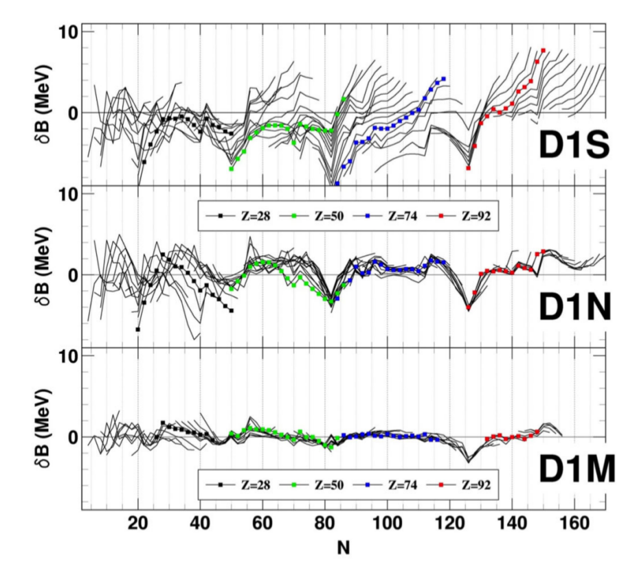
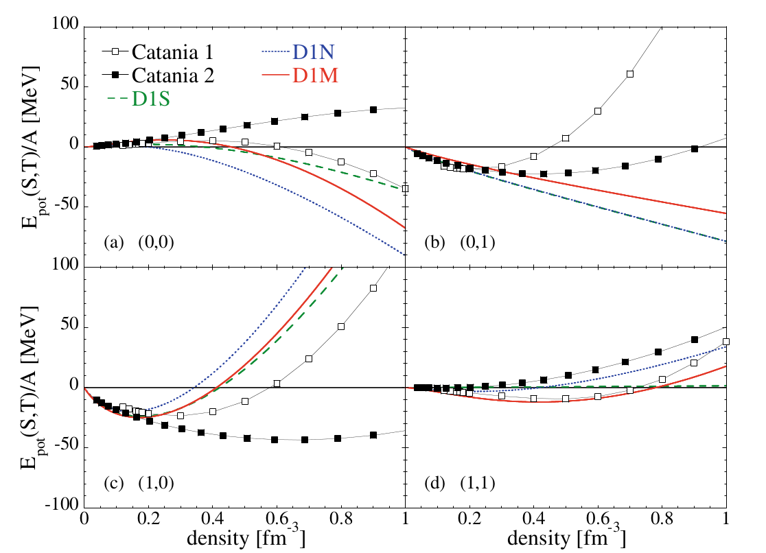
Figure 1: On the left hand side, the binding energy differences $\delta B$ in MeV is represented as a function of neutron number for the theoretical predictions of D1S, D1N and D1M. On the right hand side, the binding energy per particle $E/A$ in nuclear matter for the four different $(S,T)$ channels is shown for D1S, D1N and D1M as well as microscopic results (Catania 1 and 2). Figures taken from Ref. [44].

As a result of the adopted fitting protocol the parametrization D1M exhibits an impressive rms deviation, with respect to the measured 2149 nuclear masses [40], of 0.798 MeV. This accuracy can be compared with the best nuclear mass models. The largest deviations occur around magic numbers and, in particular, for nuclei with neutron number N $\approx$ 126. Furthermore, the neutron matter equation of state (EOS) corresponding to D1M agrees well with the one of D1N but also with the one obtained in realistic calculations [33]. Regarding the potential energy per particle for symmetric nuclear matter, the comparison with realistic Brueckner-Hartree-Fock (BHF) calculations [42, 45] reveals a fair agreement in each of the four two-body spin-isospin (S,T) channels. In particular, the set D1M accounts for the repulsive nature of the (S=0,T=0) channel as well as for the isovector splitting of the effective mass in the case of neutron-rich matter. A complete mass table has been built with the Gogny interaction D1M, for nuclei located in between the proton and the neutron drip-lines [44].

In the left panels of Fig 1 the binding energy difference between the theoretical predictions and the experimental data $\delta B$ is shown as a function of neutron number for the three most popular parametrizations of the Gogny force, namely D1S, D1N and D1M [44]. As discussed before, we clearly observe for D1S the drift in $\delta B$ for heavy systems that makes this interaction unsuitable for binding energy predictions. The parametrization D1N mostly corrects the drift of D1S for large values of N but some deviations still remain. Finally, D1M gets a very good agreement with experimental data with values of $\delta B$ much smaller than the ones of the other two interactions. On the right hand side panels, the binding energy per nucleon $E/A$ in nuclear matter is plotted as a function of the density for the four different spin, isospin (ST) channels [44]. The results are compared with the ones obtained with sophisticated many body techniques and realistic interactions. The agreement is rather good up to twice saturation density but from there one there are large deviations with some unphysical behaviors at large densities like in the (0,1) channel. The relevance of such disagreement for finite nuclei densities remains to be assessed.

The Gogny D1M force has been tested with respect to kinetic moments of inertia for Eu and Pu nuclei, giant monopole, dipole and quadrupole resonances as well as with respect to the 519 experimentally known 2${}_{1}^{+}$ excitation energies of even-even nuclei [42]. For global calculations of 2${}_{1}^{+}$ excitation energies in the framework of the symmetry-projected Generator Coordinate Method (GCM) with the Gogny D1S and D1M interactions, the reader is also referred to Ref. [46]. Previous studies for even-even [47, 48, 35, 49] but also for odd-mass [50, 51, 52, 53, 54] nuclei have shown that the parametrization D1M essentially keeps the same predictive power of the well tested D1S set to describe a wealth of low-energy nuclear structure data while improving the description of the nuclear masses. In particular, several calculations [36, 55, 56, 50] suggest that the D1M parametrization represents a reasonable starting point to describe fission properties in heavy and super-heavy nuclear systems. However, much work is still needed to further support this conclusion. Other applications of the Gogny D1M force can be found, for example, in Refs. [57, 58].

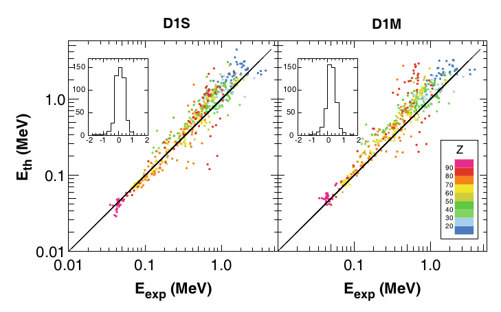
Figure 2: Comparison between the theoretical predictions for the excitation energy (in MeV) of the lowest $2^{+}$ collective state obtained with the 5DCH and the corresponding experimental data. Results for both D1S and D1M are shown. Figure taken from from Ref. [44].

In Fig 2 a comparison of the excitation energies of the collective $2^{+}$ states versus the experimental data is made both for D1S and D1M [44]. The model used to obtain the $2^{+}$ excitation energies is the five dimensional Collective Hamiltonian (5DCH) presented in Sec 6.2 that makes use of quantities obtained solely at the HFB level like potential energy surfaces, collective inertias, etc to be discussed below. In line with the discussion above, the D1S and D1M results for this finite nucleus observable are rather similar. The comparison with experimental data is rather good, specially for those states with low excitation energy that correspond to the first member of a rotational band. See  [44, 59] for further details.

2.6 D2

The most recent addition to the family of Gogny forces is the one of Ref [60] where the D2 force was proposed. The main difference with respect to D1 and other parametrizations of the D1 family is the inclusion of a finite range density dependent term. The new radial form implies that now the strongly repulsive density dependent term also contributes to the pairing field, a contribution that has to be canceled out in a delicate balance by the central potential contribution. Also, the previous dependence with the density at the center of mass coordinate has to be given up to facilitate the numerical implementation of the new force. The results of the few applications carried out so far with this new Gogny force seem to indicate a good reproduction of experimental data, at the level of other popular parametrizations like D1S or D1M. Also, other non-observable quantities like potential energy surfaces look very similar to the ones of D1S or D1M. So far, the main drawback of D2 is its heavy computer resources requirement [60] that make this force unsuited for large scale applications. In addition, the new density dependent term has still to be implemented in many of the computer codes for mean field and beyond calculations. These two facts together imply that D2 is not expected to be competitive with the D1 family of forces in the near future.

2.7 Other parametrizations

In Ref [61] several parametrizations of the Gogny force were proposed to study the relationship between the nuclear matter incompressibility parameter and the energy of breathing modes in spherical doubly magic nuclei like ⁴⁰Ca and ²⁰⁸Pb. Those parametrizations, dubbed D250, D260, D280 and D300 according to their value of the incompressibility coefficient $K_{nm}$, have not been used apart from the mentioned study and therefore their reliability remains to be assessed.

In another study [62], Farine et al introduced a new type of Gogny force, denoted D1P where a new zero range density dependent term is added to the traditional Gogny force. The main merits of D1P with respect of D1 and D1S are: (i) the agreement with experimental data on the depth of optical potentials is improved (ii) sum rules of Landau parameters are better fulfilled and (iii) a more realistic behavior for the equation of state of neutron matter is obtained. The new interaction has never been used in finite nuclei calculations and therefore their merits remain to be assessed.

The original Gogny force did not include tensor terms, which are known to modify the distribution of single particle levels around the Fermi surface. Attempts to include a tensor term have been made but the main difficulty is to find a fitting protocol to determine the parameters of the tensor part. Only the GT2 interaction by Otsuka et al including a tensor isovector contribution of Gaussian form [63] has been fully fitted but at the HF level. All the other attempts so far to incorporate a tensor term to the Gogny force were carried out without modifying the other parameters of the interaction and therefore the results obtained can be considered as exploratory. Several sets of tensor parameters have been introduced in the literature: D1ST and D1MT including a radial part based on the one of Argonne V18 [64], D1ST2a and D1ST2b including also a tensor isoscalar term but this time with a Gaussian shape [65] and also D1ST2c and D1MT2c in Ref [66] where the spin orbit strength was modified alongside with the strengths of the different channels of the tensor term. With this latter improvement it is possible to successfully reproduce the $1f_{7/2}-2p_{3/2}$ gap in the ^40-48Ca isotopic chain. All the previous results are obtained for spherical nuclei, but recently calculations in deformed nuclei with D1ST2a have been reported [67].

Another possibility to generalize the Gogny force is to increase the number of Gaussians in the central potential part to have more flexibility to adjust nuclear matter properties. This is the path taken in Ref [68] where the extra freedom was used to adjust the four spin-isospin channels of the nuclear matter potential energy to the results of realistic calculations. As in the other cases, no finite nuclei calculations have been carried so far and therefore the merits of the new proposal for finite nuclei remain to be demonstrated.

Very recently, a new variant of D1M has been proposed [69] to cure one of its most notorious drawbacks: its inability to reproduce the accepted value of two solar masses for the mass of the heaviest neutron stars. In the new parametrization, dubbed D1M^∗, the slope of the symmetry energy coefficient in nuclear matter $L$ has been fitted to a higher value (43 MeV) than the original rather low value of D1M (24.8 MeV). At the same time, all other relevant combination of parameters have been kept as to preserve the already outstanding properties of D1M, specially the properties of the pairing channel. It has to be mentioned that the D2 parametrization also gives two solar masses for the mass of neutron stars and could be considered as an alternative to D1M^∗. However, D2 is much more computationally demanding than D1M^∗.

Although not a pure Gogny force, the recent proposal of Behera et al [70] of a simple effective interaction (SEI) resembles very much the Gogny force. There are two distinctive places where the two differ: one of the ranges of the Gogny force is set to zero in SEI and the density dependence includes an additional denominator to prevent supra-luminous effects in nuclear matter. The parameters of SEI are fitted mostly to nuclear matter properties and only one (or two) are left to fit the binding energies of finite nuclei. The results obtained in finite nuclei, including binding energies, radii, deformation properties, etc are encouraging and exploratory work in other aspects of the interaction is underway.

2.8 The pairing channel of the Gogny force

The pairing interaction coming from the central part of the Gogny force has been used in many places as an alternative to zero range pairing interactions [71, 72] due to its natural ultraviolet cutoff. A systematic comparison with other alternatives in the relativistic framework can be found in Ref [73]. Due to the non-local character of this pairing interaction its numerical cost represents a large fraction of the total cost of the calculation and therefore other cheaper alternatives have been sought. In this respect we can mention the separable expansion of the two-body Gaussian interaction proposed in [74] that is widely used along with relativistic mean fields not only at the mean field level [75, 76] but even as a cheap alternative to the full Quasiparticle Random Phase Approximation (QRPA) [77]. It is also interesting to mention another separable expansion [78] valid also for the Hartree Fock part and that could be used a simpler replacement of the Gaussian.

2.9 Future improvements

It is not easy to forecast the future of the Gogny force, but there are a few things that are obvious and should be implemented in the short term. First of all, the release of the zero range radial dependence of the spin-orbit potential. This is a mostly aesthetic improvement and no big impact on any relevant observable is foreseen. A tensor term has already been introduced in the Gogny force and its impact analyzed in a variety of situations, but the tensor contribution has been introduced in a perturbative fashion, that is, no refitting of the core parameters of the force has been carried out. A version of the Gogny force with a finite range tensor term and a full refitting of the parameters at the HFB level would be highly welcome. Finally, the time-odd sector of the density dependent part of the interaction has never been explored. It is true that the time-odd fields obtained from the central, spin–orbit and Coulomb part lead to a nice reproduction of observables like moments of inertia [79, 24, 80], spin and parities of the ground state of odd mass nuclei [81, 80] or even the excitation energy of high-K isomeric states [82]. However, there are indications in the physics of odd-odd nuclei that additional time-odd fields could be required [83] in order to reproduce the rich phenomenology associated to these kind of nuclei. Finally, let us mention that in all the applications with the Gogny force proton-neutron pairing has never been considered. It is important for nuclei near $N=Z$ and considering it will require some additional constraints in the fitting protocol.

3 Mean field with the Gogny force

The mean field approximation can be considered as the simplest of all possible approximations to the fermion many body problem, as in the atomic nucleus [84]. In nuclear physics, and as a consequence of the nuclear interaction properties, the mean field is required also to incorporate those short range correlations responsible for the existence of Cooper pairs in the atomic nucleus and also responsible for the related phenomenon of nuclear super-fluidity. These two aspects are implemented in the Hartree- Fock- Bogoliubov (HFB) mean field approximation that is a generalization encompassing both the Hartree Fock (HF) and the Bardeen Cooper Schriffer (BCS) approximations into a single framework. A genuine aspect of the nuclear mean field is the ubiquitous spontaneous breaking of symmetries. This is a direct manifestation of the properties of the nuclear force that lead to mean field wave functions that can eventually break all kind of spatial or internal symmetries. Spontaneous symmetry breaking leads to mean field solutions not preserving the symmetries of the Hamiltonian like translational invariance, rotational invariance, reflection symmetry, etc. It is a consequence of the non-linear nature of the HFB equations and therefore is a consequence of the approximate mean field treatment of the problem. This aspect of the mean field could be considered as unphysical and undesirable but it turns out to be the other way around: it is a way to incorporate different kinds of correlations into a simple picture (the typical example being the BCS theory of superconductivity) and is behind the very successful concept of ”intrinsic state” in nuclear physics and the associated grouping of levels in bands connected by strong electromagnetic transitions and often found in the nuclear spectrum. Obviously, the whole idea of symmetry breaking requires some further refinement in order to obtain the physical wave functions that are labeled with quantum numbers of the symmetries of the system (angular momentum, parity, etc). How to buid laboratory-frame wave functions with the proper quantum numbers of the Hamiltonian’s symmetries out of the intrinsic states will the subject of the next section.

This characteristics leads, in a natural way, to a taxonomy of the different kind of mean field approximations based on the symmetries allowed to break in the calculations: it is common to talk about axially symmetric calculations, reflection asymmetric, triaxial etc depending on the symmetries preserved (or allowed to break) by the mean field (or the computer codes used to carry out the calculations). In the following we will make use of this terminology.

3.1 Mean field calculations with the Gogny force

General properties of the nuclear interaction require the treatment of both long range and short range correlations in the same footing. At the mean field level, this means that the traditional Hartree-Fock approximation has to be supplemented by the incorporation of short range correlations in the spirit of the BCS theory of superconductivity and super-fluidity. The incorporation of these two effects requires the introduction of the so-called HFB quasiparticle annihilation and creation operators $\beta_{\mu}$ and $\beta^{\dagger}_{\mu}$ which are expressed as linear combinations (with amplitudes $U$ and $V$) of generic creation $c^{\dagger}_{k}$ and annihilation $c_{k}$ operators that correspond to a conveniently chosen basis

$$\left(\begin{array}[]{c}\beta\\ \beta^{\dagger}\end{array}\right)=\left(\begin{array}[]{cc}U^{+}&V^{+}\\ V^{T}&U^{T}\end{array}\right)\left(\begin{array}[]{c}c\\ c^{\dagger}\end{array}\right)=W^{+}\left(\begin{array}[]{c}c\\ c^{\dagger}\end{array}\right).$$ (6)

In order to alleviate the notation we have introduced the block matrix $W$ encompassing both $U$ and $V$ in a convenient way. The associated single particle wave functions of the basis $\varphi_{k}(\vec{r})=\langle\vec{r}|c_{k}^{\dagger}|0\rangle$ can in principle be anything we want provided they span the whole Hilbert space. However, practical limitations force the use a finite subset of single particle states that only generates a limited corner of the whole Hilbert space. As a consequence, the choice of the single particle states has to be adapted to the geometry of the problem at hand and the symmetries expected to be broken by the mean field. For instance, the physics of triaxial shapes is better described in terms of wave functions breaking spherical symmetry. A typical example are those Harmonic Oscillator (HO) wave functions which are tensor product of 1D HO wave functions with different oscillator lengths along each of the spatial directions. The oscillator lengths are adapted to the size of the major axis of the matter distribution of the triaxial configuration. There is an additional constraint in the choice of the $\varphi_{k}(\vec{r})$ which is related to the need to evaluate billions of matrix elements of a two body interaction with those wave functions. In the case of the Gogny force, where the central part of the interaction is modeled in terms of a linear combination of Gaussians, the obvious choice for the basis is the set of eigen-states of the harmonic oscillator potential. Viewed from a mathematical perspective, the choice is very convenient as the Hermite polynomials entering the HO wave functions are orthogonal with respect to a Gaussian weight and therefore the evaluation of the two body matrix elements can be carried out analytically. The other terms of the interaction are either zero range (spin-orbit and density dependent part of the interaction) or can be easily expressed in terms of Gaussians as it is the case with the Coulomb potential. In appendix A we discuss the general principles guiding the efficient evaluation of matrix elements of a Gaussian two body interaction, which is central to any mean field calculation with the Gogny force. The discussion is focused on 1D harmonic oscillator wave functions which are at the heart of the triaxial representation of the HO wave functions [26]. Other possibilities involving the 2D harmonic oscillator [85, 86] or even the 3D one [11] rely on the same principles and will not be discussed in detail.

The Bogoliubov transformation of Eq (6) has to preserve the commutation relations of creation and annihilation quasiparticle operators. This requirement restricts the form of the $W$ matrices to those satisfying some sort of unitarity constraint

$$W^{\dagger}\sigma W^{*}=\sigma$$ (7)

where

$$\sigma=\left(\begin{array}[]{cc}0&\mathbb{I}\\ \mathbb{I}&0\end{array}\right)$$ (8)

is a block matrix with the same block structure as $W$. Given a set of quasiparticle operators satisfying the canonical commutation relations, the associated mean field HFB wave function $|\varphi\rangle$ is defined by the condition $\beta_{\mu}|\varphi\rangle=0$ that is fulfilled by the product state

$$|\varphi\rangle=\prod_{\mu}\beta_{\mu}|-\rangle$$ (9)

where the product extends to those labels $\mu$ for which the product is non-zero. Finally, the $U$ and $V$ amplitudes of the Bogoliubov transformation (or the $W$ amplitudes) are determined by the Ritz variational principle on the HFB energy $E_{\mathrm{HFB}}=\langle\varphi|\hat{H}|\varphi\rangle/\langle\varphi|\varphi\rangle$. The Hamiltonian is the sum of a one body kinetic energy term plus a two body potential term that is written in second quantization form as

$$\hat{H}=\sum_{ij}t_{ij}c^{\dagger}_{i}c_{j}+\frac{1}{4}\sum_{ijkl}\bar{\nu}_{ijkl}c^{\dagger}_{i}c^{\dagger}_{j}c_{l}c_{k}$$ (10)

with $\bar{\nu}_{ijkl}$ the antisymmetrized two body matrix element $\bar{\nu}_{ijkl}=\langle ij|v(1,2)|kl\rangle-\langle ij|v(1,2)|lk\rangle$. Very often the minimization of the energy is restricted to fulfill some constraints on the mean value of some operators $\hat{O}_{i}$ like the quadrupole or octupole moments of the mass distribution. These constraints have to be considered along with the traditional constraint on particle number $\langle N\rangle=N$ and $\langle Z\rangle=Z$ characteristic of the HFB theory. In order to handle this situation the introduction of Lagrange multipliers $\lambda_{i}$ is required. The quantity to be minimized becomes

$$E_{\mathrm{HFB}}^{\prime}=\langle\varphi|\hat{H}^{\prime}|\varphi\rangle/\langle\varphi|\varphi\rangle$$ (11)

where

$$\hat{H}^{\prime}=\hat{H}-\sum_{i}\lambda_{i}\hat{O}_{i}$$ (12)

It is now possible to carry out an unconstrained minimization of $E_{\mathrm{HFB}}^{\prime}(\lambda_{1},\lambda_{2},\ldots)$ but fixing the values of the chemical potentials $\lambda_{i}$ by requiring that the mean value of the constraining operators is equal to the desired value of the constraints $\langle\varphi|\hat{O}_{i}|\varphi\rangle=o_{i}$.

Before proceeding with the application of the variational principle to $E_{\mathrm{HFB}}^{\prime}$ we have to overcome an additional problem: the $U$ and $V$ amplitudes are not linearly independent due to the constraint of Eq (7) and they therefore cannot be used as independent variational parameters. A set of variables which are linearly independent is provided by the Thouless theorem [87, 84] that gives the most general form of an HFB state $|\varphi(Z)\rangle$ in terms of some linearly independent complex parameters $Z_{\mu\mu^{\prime}}$ (with $\mu^{\prime}>\mu$ ) and a reference HFB state $|\varphi_{0}\rangle$

$$|\varphi(Z)\rangle=\eta(Z,Z^{*})\exp\left(\sum_{\mu<\mu^{\prime}}Z_{\mu\mu^{\prime}}\beta_{\mu}^{+}\beta_{\mu^{\prime}}^{+}\right)|\varphi_{0}\rangle$$ (13)

where $\eta(Z,Z^{*})$ is a normalization constant such that $\langle\varphi(Z)|\varphi(Z)\rangle=1$. The only restriction on $|\varphi(Z)\rangle$ is that it must have a non-zero overlap with $|\varphi_{0}\rangle$. As it is customary, we will use as free parameters $Z$ and $Z^{*}$ instead of $\Re(Z)$ and $\Im(Z)$. The relation between the Bogoliubov wave functions $U(Z)$ and $V(Z)$ corresponding to $|\varphi(Z)\rangle$ and the $U_{0}$ and $V_{0}$ corresponding to $|\varphi_{0}\rangle$ is given by [88]

$$U(Z) = (U_{0}+V_{0}^{*}Z^{*})\left[L^{-1}\right]^{\dagger}$$ (14)

$$V(Z) = (V_{0}+U_{0}^{*}Z^{*})\left[L^{-1}\right]^{\dagger}$$ (15)

where the matrix $L[Z,Z^{*}]$ is the Choleski decomposition of the positive definite matrix $I+Z^{T}Z^{*}$, i.e.,

$$LL^{\dagger}=I+Z^{T}Z^{*}$$ (16)

where $I$ is the unity matrix. The Choleski decomposition is nothing but the “square root” of the matrix $I+Z^{T}Z^{*}$. Using the Thouless parametrization, the HFB energy is given by a function of the linearly independent complex $Z$ and $Z^{*}$ parameters

$$E^{\prime}(Z,Z^{*})=\frac{\langle\varphi(Z)|H^{\prime}(Z,Z^{*})|\varphi(Z)\rangle}{\langle\varphi(Z)|\varphi(Z)\rangle}$$ (17)

The Gogny force is state dependent through the density dependent term that depends on the mass density of the corresponding state $|\varphi(Z)\rangle$. This is the reason why in the above expression we have considered that the Hamiltonian explicitly depends on the $Z$ and $Z^{*}$ amplitudes and this dependence has to be taken into account in the variational principle. As the $Z$ and $Z^{*}$ amplitudes are independent variational parameter, the Ritz variational principle becomes

$$\frac{\partial E(Z,Z^{*})}{\partial Z_{\mu\mu^{\prime}}}=\frac{\partial E(Z,Z^{*})}{\partial Z_{\mu\mu^{\prime}}^{*}}=0$$ (18)

For practical reasons it is better to define the HFB amplitudes which are a solution of the Ritz variational principle equation, as those corresponding to the reference HFB amplitude of the Thouless theorem $|\varphi_{0}\rangle$ and therefore the derivatives in Eq (18) are to be evaluated at $Z=Z^{*}=0$. Using the expression for the partial derivative of $|\varphi(Z)\rangle{}$

$$\frac{\partial}{\partial Z_{\mu\mu^{\prime}}}|\varphi(Z)\rangle=\beta_{\mu}^{+}\beta_{\mu^{\prime}}^{+}|\varphi_{0}\rangle+O(Z,Z^{*})$$ (19)

we obtain

$$\frac{\partial E^{\prime}(Z,Z^{*})}{\partial Z_{\mu\mu^{\prime}}}_{|Z=0}=\langle\varphi_{0}|H^{\prime}(0,0)\beta_{\mu}^{+}\beta_{\mu^{\prime}}^{+}|\varphi_{0}\rangle{}+\left\langle\frac{\delta H^{\prime}}{\delta Z_{\mu\mu^{\prime}}}\right\rangle_{|Z=0}=0$$ (20)

which is the HFB equation for density dependent forces. Traditionally, the dependence on $Z$ and $Z^{*}$ of the Hamiltonian comes through a density dependent term depending on the spatial density

$$\rho(\vec{R})=\langle\varphi(Z)|\hat{\rho}(\vec{R})|\varphi(Z)\rangle$$ (21)

where $\hat{\rho}(\vec{R})=\sum_{i=1}^{A}\delta(\vec{r}_{i}-\vec{R})$ is the standard matter density operator and $\vec{R}=\frac{1}{2}(\vec{r}_{1}+\vec{r}_{2})$ is the center of mass coordinate. Then

$$\frac{\partial\rho}{\partial Z_{\mu\mu^{\prime}}}_{|Z_{\mu\nu}=0}=\langle\varphi_{0}|\hat{\rho}(\vec{R})\beta_{\mu}^{+}\beta_{\mu^{\prime}}^{+}|\varphi_{0}\rangle$$ (22)

and therefore

$$\frac{\partial H^{\prime}}{\partial Z_{\mu\mu^{\prime}}}=\frac{\partial\rho}{\partial Z_{\mu\mu^{\prime}}}\frac{\partial H^{\prime}}{\partial\rho}=\langle\varphi_{0}|\hat{\rho}(\vec{R})\beta_{\mu}^{+}\beta_{\mu^{\prime}}^{+}|\varphi_{0}\rangle\frac{\partial H^{\prime}}{\partial\rho}$$ (23)

In the above expression both $\langle\varphi_{0}|\widehat{\rho}(\vec{R})\beta_{\mu}^{+}\beta_{\mu^{\prime}}^{+}|\varphi_{0}\rangle$ and $\frac{\delta H^{\prime}}{\delta\rho}$ have to be understood as operators in the variable $\vec{R}$ and, therefore, $\frac{\delta H^{\prime}}{\delta Z_{\mu\mu^{\prime}}}$ has to be treated as a two body operator in the evaluation of the mean values of Eq (20). Inserting the result of Eq (23) in Eq (20) we finally arrive to the HFB equation for density dependent forces in standard form

$$H^{\prime 20}_{\mu\mu^{\prime}}\equiv\langle\varphi_{0}|H^{\prime}\beta_{\mu}^{+}\beta_{\mu^{\prime}}^{+}|\varphi_{0}\rangle+\left\langle\langle\varphi_{0}|\hat{\rho}(\vec{R})\beta_{\mu}^{+}\beta_{\mu^{\prime}}^{+}|\varphi_{0}\rangle\frac{\partial H^{\prime}}{\partial\rho}\right\rangle=0$$ (24)

In the present context, the Lagrange multipliers $\lambda_{i}$ are defined by the condition that the gradient of the density dependent Routhian has to be perpendicular to the gradient of the constraints

$$O^{20}_{j\,\mu\mu^{\prime}}=\langle\varphi_{0}|\hat{O}_{j}\beta_{\mu}^{+}\beta_{\mu^{\prime}}^{+}|\varphi_{0}\rangle$$ (25)

That is

$$\sum_{\mu\mu^{\prime}}H^{\prime 20}_{\mu\mu^{\prime}}O^{20}_{j\,\mu\mu^{\prime}}=\sum_{\mu\mu^{\prime}}H^{20}_{\mu\mu^{\prime}}O^{20}_{j\,\mu\mu^{\prime}}-\sum_{i}\lambda_{i}\sum_{\mu\mu^{\prime}}O^{20}_{i\,\mu\mu^{\prime}}O^{20}_{j\,\mu\mu^{\prime}}=0$$ (26)

what represents a linear system of equations for the unknown $\lambda_{i}$. The first term of the gradient in Eq (24) can be easily computed by using the quasi-particle representation of the Hamiltonian operator while the second needs further treatment. Using the second quantization form of the density operator

$$\widehat{\rho}(\vec{R})=\sum_{ij}f_{ij}(\vec{R})c_{i}^{+}c_{j}$$ (27)

where $f_{ij}(\vec{R})=\langle i|\delta(\vec{r}-\vec{R})|j\rangle=\varphi^{*}_{i}(\vec{R})\varphi_{j}(\vec{R})$, the last term of Eq. (24) can be written as

$$\sum_{ij}\langle\varphi_{0}|c_{i}^{\dagger}c_{j}\beta_{\mu}^{\dagger}\beta_{\mu^{\prime}}^{\dagger}|\varphi_{0}\rangle\left\langle f_{ij}(\vec{R})\frac{\delta H^{\prime}}{\delta\rho}\right\rangle$$ (28)

which suggests the definition of the one body operator

$$\widehat{\partial\Gamma}=\sum_{ij}\partial\Gamma_{ij}c_{i}^{+}c_{j}$$ (29)

with matrix elements

$$\partial\Gamma_{ij} = \left\langle\frac{\delta H^{\prime}}{\delta\rho}f_{ij}(\vec{R})\right\rangle$$

$$= \frac{1}{4}\sum_{klmn}\langle kl|\frac{\delta H^{\prime}}{\delta\rho}f_{ij}(\vec{R})|\widetilde{mn}\rangle\left(\rho_{nl}\rho_{mk}-\rho_{ml}\rho_{nk}-\kappa_{mn}\kappa^{*}_{kl}\right)$$

requiring antisymmetrized two body matrix elements of the rearrangement term. With this definition, the last term of Eq. (24) becomes

$$\langle\varphi_{0}|\widehat{\partial\Gamma}\beta_{\mu}^{+}\beta_{\mu^{\prime}}^{+}|\varphi_{0}\rangle$$ (31)

which shows that the calculation of the gradient of the Routhian for density dependent forces proceeds in the same way as for standard forces except for the fact that an additional density dependent one body operator $\hat{\partial\Gamma}$ has to be added to the Hamiltonian. The calculation of the gradient $G$ now follows the standard procedure and we finally obtain

$$G_{\mu\mu^{\prime}}=H^{\prime 20}_{\mu\mu^{\prime}}=H^{20}_{\mu\mu^{\prime}}-\sum_{i}\lambda_{i}O^{20}_{i\,\mu\mu^{\prime}}$$ (32)

with

$$H^{20}_{\mu\mu^{\prime}}=\left(U^{+}hV^{*}-V^{+}h^{T}U^{*}+U^{+}\Delta U^{*}-V^{+}\Delta^{*}V^{*}\right)_{\mu\mu^{\prime}}$$ (33)

given in terms of

$$h_{ij} = t_{ij}+\partial\Gamma_{ij}+\Gamma_{ij}$$ (34)

$$\Gamma_{ij} = \sum_{qq^{\prime}}\widetilde{\upsilon}_{iqjq^{\prime}}\rho_{q^{\prime}q}$$ (35)

$$\partial\Gamma_{ij} = \frac{1}{4}\sum_{klmn}\langle kl|\frac{\delta H^{\prime}}{\delta\rho}f_{ij}(\vec{R})|\widetilde{mn}\rangle\left(\rho_{nl}\rho_{mk}-\rho_{ml}\rho_{nk}-\kappa_{mn}\kappa^{*}_{kl}\right)$$ (36)

$$\Delta_{ij} = \frac{1}{2}\sum_{qq^{\prime}}\widetilde{\upsilon}_{ijq^{\prime}q}\kappa_{q^{\prime}q}$$ (37)

As the mean value of the HFB Routhian only depends upon the standard density matrix $\rho_{ij}$ and pairing tensor $\kappa_{ij}$, it only depends upon the two first transformations of the Bloch-Messiah decomposition of the $U$ and $V$ amplitudes [89, 90] (see [84] for a detailed discussion). As a consequence, the HFB equation Eq. 24 only determines the Bogoliubov transformation up to an unitary transformation among the quasiparticles (the third transformation of the Bloch-Messiah theorem). To fix this arbitrary unitary transformation it is customary to introduce an additional imposition to the Bogoliubov transformation: namely that the ${H^{\prime}}^{11}_{\mu\nu}$ matrix, defined as

$$H^{\prime 11}_{\mu\mu^{\prime}}=H^{11}_{\mu\mu^{\prime}}-\sum_{i}\lambda_{i}O^{11}_{i\,\mu\mu^{\prime}}$$ (38)

with

$$H^{11}_{\mu\nu}=\left(U^{+}hU-V^{+}h^{T}V+U^{+}\Delta V-V^{+}\Delta^{*}U\right)_{\mu\mu^{\prime}},$$ (39)

has to be diagonal. The eigenvalues of this matrix are called quasiparticle energies and denoted by $E_{\mu}$. For non-density dependent forces they represent an approximation to the energy gain of the odd system represented by the non-self-consistent wave function $\beta^{+}_{\mu}|\varphi\rangle$ with respect to the corresponding even one $|\varphi\rangle$

$$E_{\mu}\approx\langle\varphi|\beta_{\mu}H^{\prime}\beta^{\dagger}_{\mu}|\varphi\rangle-\langle\varphi|H^{\prime}|\varphi\rangle$$ (40)

in which the two quasiparticle interaction terms of the Hamiltonian have been dropped. The first impression looking at the previous equation is that one should use $H$ instead of $H^{\prime}$ in it. However, the use of $H^{\prime}$ in the definition of $E_{\mu}$ implies that, at first order in perturbation theory, we are correcting for the fact that the mean values of the constraining operators for the state $\beta^{\dagger}_{\mu}|\varphi\rangle$ are not the same as those of $|\varphi\rangle$ (the correct ones).

For density dependent forces it has to be taken into account that the Hamiltonian used in the evaluation of the energy of the odd system differs from the one used in the calculation of the even one as the former depends on the density of the odd system

$$\rho^{\rm odd}(\vec{R})_{\mu}=\langle\varphi|\beta_{\mu}\hat{\rho}\beta^{\dagger}_{\mu}|\varphi\rangle=\rho^{\rm even}+\delta\rho_{\mu}$$ (41)

where

$$\delta\rho(\vec{R})_{\mu}=\sum_{ij}f_{ij}(\vec{R})(U^{*}_{i\mu}U_{j\mu}-V^{*}_{j\mu}V_{i\mu})$$ (42)

As $\delta\rho_{\mu}$ is the change on the density coming from the addition of a particle it is small compared with the total density of the system and therefore it is reasonable to expand the density dependent Hamiltonian of the odd system around the one of the even system as

$$\hat{H}(\rho^{\rm odd}_{\mu})=\hat{H}(\rho_{0})+\frac{\delta H}{\delta\rho}\delta\rho_{\mu}+\ldots$$ (43)

With this expansion the energy of the odd system can be evaluated as

$$\langle\varphi_{0}|\beta_{\mu}\hat{H}(\rho^{\rm odd}_{\mu})\beta^{\dagger}_{\mu}|\varphi_{0}\rangle = \langle\varphi_{0}|\beta_{\mu}\hat{H}(\rho_{0})\beta^{\dagger}_{\mu}|\varphi_{0}\rangle+\langle\varphi_{0}|\beta_{\mu}\frac{\delta\hat{H}}{\delta\rho}\delta\rho_{\mu}\beta^{\dagger}_{\mu}|\varphi_{0}\rangle$$

$$= \langle\varphi_{0}|\hat{H}(\rho_{0})|\varphi_{0}\rangle+H^{11}_{0_{\mu\mu}}+\langle\varphi_{0}|\beta_{\mu}\Delta\left[\frac{\delta\hat{H}}{\delta\rho}\delta\rho_{\mu}\right]\beta^{\dagger}_{\mu}|\varphi_{0}\rangle$$

where $H^{11}_{0_{\mu\mu}}$ is computed with the wave functions of $|\varphi_{0}\rangle$

$$H^{11}_{0_{\mu\mu}}=\left(U^{+}hU-V^{+}h^{T}V+U^{+}\Delta V-V^{+}\Delta^{*}U\right)_{\mu\mu}$$ (45)

and contains in its definition the rearrangement potential. The remaining term ( in which the definition $\Delta\hat{O}=\hat{O}-\langle\varphi_{0}|\hat{O}|\varphi_{0}\rangle$ has been used) represents the interaction of the quasiparticle with the change induced by itself in the density. It is comparable with the magnitude of the quadratic terms in $\delta\rho_{\mu}$ neglected in the expansion of the Hamiltonian and therefore should not be considered.

The conditions $H^{\prime\,20}_{\mu\mu^{\prime}}=0$ and $H^{\prime\,11}_{\mu\mu^{\prime}}=E_{\mu}\delta_{\mu\mu^{\prime}}$ can be written in compact form as

$$\left(\begin{array}[]{cc}H^{\prime\,11}&H^{\prime\,20}\\ -H^{\prime\,20*}&-H^{\prime\,11}\end{array}\right){}=W\left(\begin{array}[]{cc}h&\Delta\\ -\Delta^{*}&-h^{*}\end{array}\right){}W^{\dagger}=\left(\begin{array}[]{cc}E&0\\ 0&-E\end{array}\right){}$$ (46)

Introducing the block Hamiltonian matrix

$$\mathcal{H}=\left(\begin{array}[]{cc}h&\Delta\\ -\Delta^{*}&-h^{*}\end{array}\right){}$$ (47)

and the block density

$$\mathcal{R}=\left(\begin{array}[]{cc}\rho&\kappa\\ -\kappa^{*}&-\rho^{*}\end{array}\right){}$$ (48)

the condition of Eq 46 is expressed as

$$\mathcal{H}W=W\left(\begin{array}[]{cc}E&0\\ 0&-E\end{array}\right){}$$ (49)

that is the traditional form of the HFB equation. Please note, that the $W$ transformation also brings $\mathcal{R}$ to diagonal form

$$W^{\dagger}\mathcal{R}W^{*}=\left(\begin{array}[]{cc}0&0\\ 0&\mathbb{I}\end{array}\right){}$$ (50)

and therefore Eq (49) implies that $\mathcal{H}$ must commute with $\mathcal{R}$ at the self-consistent solution of the HFB equation.

The HFB equation is a non-linear equation where the matrix to be diagonalized $\mathcal{H}$ depends upon the eigenvectors $W$ through the density matrix and pairing tensor. Therefore, the HFB equation is not an standard eigenvalue problem. The best way to tackle the solution of the HFB equation is to solve it iteratively: starting with a reasonable guess for $U$ and $V$, the density $\rho$ and pairing tensor $\kappa$ and the corresponding HF $h$ and pairing $\Delta$ fields are computed and then used to build the generalized Hamiltonian $\mathcal{H}$. The Hamiltonian is diagonalized to obtain a new set of $U$ and $V$ amplitudes. The process is repeated iteratively until convergence is achieved (i.e. the input $U$ and $V$ are the same as the output ones). This is the preferred approach by the Bruyéres-Le-Châtel group. To make it converge, some kind of “slowing down” strategy has to be implemented in the iterative procedure. Traditionally, this “slowing down” is implemented by mixing the $U^{i+1}$ and $V^{i+1}$ amplitudes with the previous iteration’s ones $U^{i}$ and $V^{i}$ by means of some add-hoc mixing parameter $\eta$. The proper choice of $\eta$ requires some experience and the consideration of the type of calculation at hand. There is an alternative to this procedure based on the equivalence between the HFB equation and the variational principle over the HFB mean value of the Routhian: the HFB amplitudes solving the HFB equation are those that minimize the HFB mean value of the Routhian. Therefore, the HFB problem can be considered as a minimization problem with a very large set of variational parameters $Z$ and $Z^{*}$. This is one of the classical problems in numerical analysis and the usual numerical techniques used in this case can be invoked: the gradient method [91], the conjugate gradient method [88] and the (approximate) second order Newton-Rampson method [29]. The most notorious advantages of any variant of the gradient method versus the iterative one are the easy handling of multiple constraints that is often required in practical applications like fission or the determination of potential energy surfaces, the much lower iteration count and, finally, the guarantee that the method always converges to a solution (that might not be the optimal one).

In the case of the Gogny force and, at variance with similar type of calculations using the Skyrme EDF, the pairing field $\Delta$ is computed from the same interaction used in the central particle-hole (p-h) channel. The finite range of the central potential makes unnecessary any kind of cut-off or restriction on the active configuration space. The pairing field gets contributions from the central potential and the spin-orbit term. The density dependent term does not contribute to the pairing channel in the traditional family of D1 like parametrizations (D1, D1S, D1N, etc) due to its zero range, the specific spin structure (the $x_{1}$ parameter is one) and the fact that the wave function is a product of independent proton and neutron wave functions. This is not the case for more recent parametrizations of the Gogny force with a finite range density dependent potential [60] that belong to the D2 family of next generation Gogny forces. The spin-orbit contribution to the pairing field is often neglected but the anti-pairing field coming from the two body kinetic energy correction included in the definition of the Gogny force is fully taken into account. Let us finally mention that the explicit central potential contribution to $\Delta$ is similar in structure to the HF exchange contribution to $h$ and shares its computational complexity.

In addition to the Gogny force, the interaction used to solve the HFB equation includes the Coulomb potential among protons and a two body kinetic energy correction. The Coulomb potential contributes in principle to the direct, exchange and pairing fields, but it is customary to treat exactly only the direct contribution whereas the exchange contribution is replaced by the Slater approximation and the Coulomb anti-pairing field is simply neglected. The relative importance of the exact Coulomb exchange and Coulomb anti-pairing effect has been discussed in detail in the context of particle number symmetry restoration and high spin physics at the HFB level in Ref [92]. Although Coulomb exchange is usually well described by the Slater approximation, the impact of neglecting Coulomb anti-pairing can be rather dramatic in quantities like collective inertias or the moment of inertia of high spin states. On the other hand, the contribution of the two body kinetic energy correction to both the HF and pairing fields is fully taken into account. The two body kinetic energy correction contribution to pairing is repulsive and yields to a rather large anti-pairing effect that is compensated by the central potential contribution.

For the implementation of all these techniques in the form of computer codes see appendix B.

Mean field calculations with the Gogny force go back to the mid seventies. The first paper appearing in a regular journal was a HF calculation of deformation properties in the Sm isotopes [19] where it was shown that the recently proposed Gogny D1 interaction was able to reproduce quadrupole deformation properties of heavy nuclei. This early paper was followed by a beyond-mean field calculation of the charge density of ⁵⁸Ni [93]. In both cases quadrupole deformation was allowed and an axially symmetric HO basis was used to expand the HF amplitudes. The full consideration of the HFB theory was performed in the seminal calculation by J. Decharge and D. Gogny of spherical nuclei [20] where the D1 parametrization of the force was used to study semi-magic nuclei and their pairing properties along isotopic chains. For mean field calculations using the Skyrme EDF or relativistic lagrangians the reader is refered to the review paper of Ref [94].

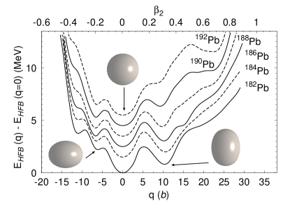
Figure 3: Potential energy surfaces given as a function of the axial quadrupole moment $q$ in barns for several neutron deficient lead isotopes showing the phenomenon of triple shape coexistence. The real shape of the nucleus for each of the three minima is also shown. Figure adapted from Ref. [95].

At the mean field level it is customary to carry out constrained calculations where the target wave function is required to produce specific values of the mean values of some observables like the quadrupole, octupole, etc mass moments. In this way, the so-called “potential energy surfaces” (PES) are obtained. They are linked to the dynamics of the associated collective degree of freedom (represented by the constrained operator: quadrupole, octupole, etc). Typical calculations of this kind are those studying the PES as a function of the axial quadrupole moment in order to identify the ground state’s quadrupole deformation or the existence of shape coexistence between prolate or oblate minima (some times saddle points). A typical example is that of the triple shape coexistence in neutron deficient lead isotopes revealing three minima, one prolate, one oblate and other spherical [95]. The PES corresponding to the relevant nuclei is shown in Fig 3 as a function of the quadrupole moment. Triple shape coexistence is observed in most of the nuclei displayed in the Figure and can be connected with three low lying $0^{+}$ states, like the ones experimentally identified in ¹⁸⁶Pb [96].

These kind of PES calculations are also useful to identify the existence of super-deformed [97] or even hyper-deformed intrinsic states [86]. Quadrupole deformed axially symmetric PESs are also very common in the description of fission as they allow for the description of the “potential energy” felt by the nucleus in its way down to fission. In this case, reflection symmetry is allowed to break in order to describe asymmetric fission, where the mass of the two resulting fragments is not equal.

The calculation of PES using as collective variable the axial octupole moment $Q_{30}$ has permitted to characterize octupole correlations in nuclei. After some years of debate (see, for instance, [98]), the octupole deformed character of some nuclei like ²²⁴Ra [99] or ^144-146Ba [100, 101] has been unambiguously established experimentally. The coupling between the axially symmetric quadrupole and octupole degrees of freedom has been analyzed at the mean field level in Refs [102, 47]. A weak but not neglegible coupling is found in most of the cases studied.

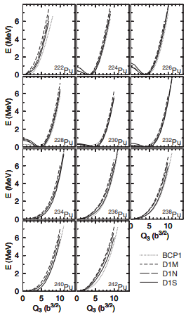
Figure 4: HFB potential energy surfaces computed with three variants of the Gogny force (D1S, D1N, D1M) and the BCP1 [103] energy density functional are plotted as a function of the axial octupole moment for several isotopes of Pu. Figure adapted from Ref. [48].

Systematic mean field calculations exploring the existence of octupole deformation in the ground state of even-even nuclei have been carried out with D1S, D1N and D1M in Ref [29] in the context of a beyond mean field calculation. Here, it was found that octupole deformation is only present in a few actinides around Ra, a few rare earth around Ba and a few $A\approx 90$ nuclei around Zr. In Ref [48] another calculation in the actinide region and taking into account other functionals came to the same conclusion. In Fig 4 a sample of those calculations is given. Potential energy curves are plotted as a function of the axial octupole moment $Q_{30}$ for a few relevant Pu isotopes. It is found that irrespective of the interaction used, the isotopes from ²²⁴Pu to ²³²Pu have an octupole deformed ground state. The deepest minimum occurs for ²²⁶Pu with a depth that slightly depends on the force used but is of the order of 1 MeV.

In order to look for triaxial deformed minima, another component of the quadrupole tensor has to be taken into account in addition to $Q_{20}$. The resulting ”triaxial shapes” are characterized by the $\beta$ and $\gamma$ shape parameters.

$$\beta = \sqrt{\frac{20\pi}{9}}\frac{\sqrt{Q_{20}^{2}+2Q_{22}^{2}}}{r_{0}^{2}A^{5/3}}$$ (51)

$$\tan\gamma = \frac{\sqrt{2}Q_{22}}{Q_{20}}$$ (52)

The first calculation with the Gogny force including triaxiality was presented in Ref [26] where also details on how to compute the matrix elements of the Gogny force in a triaxial HO basis are given. In the triaxial case, PESs become the popular $\beta-\gamma$ planes that are very helpful in the interpretation of experimental results. This $\beta-\gamma$ planes are also essential ingredients in the 5DCH (see Sec 6.2 for details) to be discussed below as well as in the determination of the parameters of the interacting boson model (see Sec 4.2). Triaxial deformation also plays a relevant role in the reduction, by a couple of MeV, of the first fission barrier height in the Actinides [26, 24]. This reduction improves substantially the agreement with experimental data and helps to reduce the rather long predictions for the spontaneous fission half lives. An example of $(\beta,\gamma)$ potential energy surfaces is given in Fig 5 for the nuclei ¹⁵⁰Sm and ¹⁵²Sm in the form of a polar contour plot. The two nuclei show a prolate ground state with deformations $\beta=0.2$ and $\beta=0.23$, respectively as well as oblate minima that are connected to the prolate minima through a path that goes along triaxial shapes. The barrier for this path is, in the two cases, much lower that the one corresponding to the path going through spherical shapes.

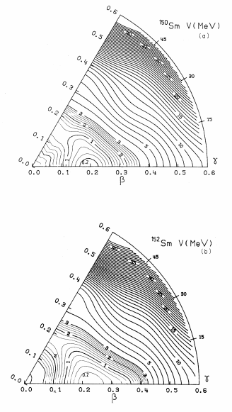
Figure 5: HFB $\beta-\gamma$ potential energy surfaces for the A=150 and 152 isotopes of Sm computed with the Gogny D1S force. Contour lines are drawn every 0.2 MeV for energies between 0 and 3 MeV and every 1 MeV for higher energies. Figure taken from Ref.[26].

High spin physics can also be described in the mean field framework by using the Cranked HFB method where an additional constraint is introduced on the mean value of the $\hat{J}_{x}$ operator [104]

$$\langle\hat{J}_{x}\rangle=\sqrt{J(J+1)-\langle\hat{J}_{z}^{2}\rangle}$$ (53)

The last term $\langle\hat{J}_{z}^{2}\rangle$ is often neglected in practical applications for even-even nuclei where it tends to be rather small compared to $J(J+1)$. By solving the HFB equation with this constraint a Lagrange multiplier $\omega$ has to be introduced. As the Lagrange multiplier corresponds to the derivative of the energy with respect to the constraint, it can be interpreted as the angular velocity of the rotating nucleus. The Cranked HFB can be derived (see below) by starting with an angular momentum projected theory where the intrinsic wave function is searched for as to minimize the projected energy (Variation After Projection, VAP) while assuming the strong deformation limit for the intrinsic state [105]. Another characteristic feature of the Cranked HFB is the time-odd character of the constraining operator that leads to the breaking of time reversal invariance even in even-even nuclei. The first applications of the Cranking method with realistic effective interactions go back to the early seventies when the method was implemented with the Pairing+Quadrupole hamiltonian [104] and also with Skyrme interactions [106]. The solution of the Cranked HFB equation was first implemented in a computer code with the Gogny force a few years later in Ref [30] in order to study the evolution of rotational bands with spin and the backbending phenomenon. It turns out that the moment of inertia of a rotational band as obtained with the Cranked HFB (the Thouless-Valatin moment of inertia [107]) is a good observable to test the pairing channel of the interaction and there have been several thorough studies in this respect [79, 24, 80]. An example of rotational band in a normal deformed nucleus ¹⁶⁴Er showing the phenomenon of backbending is shown in the left-hand side panels of Fig 6 where the $\gamma$ ray energy $\Delta E_{\gamma}(I)=E(I)-E(I-2)$ is plotted vs the spin $I$. Also the static moment of inertia $\mathcal{J}$ is plotted as a function of the square of the angular velocity $\omega$. In both plots the phenomenon of backbending (the crossing of two rotational bands with different structures) is clearly seen as a sudden dip in the case of $\Delta E(I)$ and as a back-bending curve in the case of $\mathcal{J}$. Super-deformed intrinsic states also produce beautiful rotational bands that have been the subject of systematic studies with the Gogny force [97, 108]. The interplay between angular momentum and octupole correlations leading to the concept of alternating parity rotational bands has been analyzed in [109, 110]. An example of alternating parity bands (requiring projection to good parity, see Sec 5.2 below) is given in the right panel of Fig 6 where the energy of the members of the positive and negative parity rotational bands are plotted as a function of the angular momentum for several rare earth isotopes. At low spins the four nuclei are not octupole deformed and the positive and negative parity bands are well separated. However, as the spin increases, permanent octupole deformation develops in the intrinsic state. As a consequence, the excitation energy of the negative parity state with respect to the positive parity one becomes very small (see Sec 5.2 below) and the two rotational bands interleave.

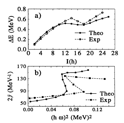
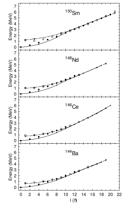
Figure 6: On the left hand side, upper panel the $\gamma$ ray energy $\Delta E_{\gamma}(I)=E(I)-E(I-2)$ is plotted vs the spin $I$ for the rotational band of the nucleus ¹⁶⁴Er. In the lower panel, the static moment of inertia $\mathcal{J}$ for the same nucleus is plotted vs the square of the angular velocity $\omega$ to show the phenomenon of backbending. On the right hand side panel the $\gamma$ ray energy of the positive and negative parity rotational bands of various rare earth isotopes is plotted as a function of angular momentum $I$. Figure adapted from Ref.[30]  [110].

Another situation where the time-reversal symmetry of the wave function is explicitly broken is in the description of odd mass, or odd-odd mass nuclei due to the presence of unpaired nucleons. In the HFB framework, odd-A nuclei require the introduction of the so-called “blocked” HFB states

$$|\Psi_{\mu}\rangle=\beta_{\mu}^{\dagger}|\Psi_{0}\rangle$$ (54)

where $|\Psi_{0}\rangle$ is the wave function of an even system and $\beta_{\mu}^{\dagger}$ is the quasiparticle creation operator on the quantum state characterized by the label $\mu$. In order to define in a more precise way the concepts just to be discussed, it is convenient to introduce the concept of “number parity”. It can easily be proven by going to the BCS representation with the Bloch-Messiah theorem [89] that any HFB wave function can be decomposed as a linear combination of wave functions with definite number of particles. The decomposition is such that wave functions with an even number of particles cannot be mixed with those with an odd number of particles. As a consequence, we can catalog any HFB intrinsic state in terms of the “number parity”, even or odd, according to the parity of the number of particles entering into its decomposition. For instance, a HFB wave function has “even number parity” if it is decomposed as a linear combination of good particle number states containing only even number of particles. In the same way “odd number parity” states are defined. A fully paired HFB state with a BCS like structure in the canonical basis has even number parity. In principle, HFB states with even number parity (both for protons and neutrons) could only be used to describe even-even nuclei. Using this language, $|\Psi_{0}\rangle$ in Eq (54) is an even number parity state, whereas, by construction $|\Psi_{\mu}\rangle$ has odd number parity and is only suited to describe odd mass systems.

The “blocked” HFB state of Eq 54 is also a HFB state, as it is the vacuum of the set of quasiparticle operators $\beta_{1},\ldots,\beta_{\mu}^{\dagger},\ldots$ [111]. As $\beta_{\mu}^{\dagger}$ now plays the role of $\beta_{\mu}$ and both states can be obtained from the other by a convenient exchange of the $\mu-th$ column of the $U$ and $V$ amplitudes it is not surprising that the “blocked” HFB method is essentially the same as the traditional, fully paired one, but performing the $U$ and $V$ column exchange in the appropriate place [111]. For instance, the traditional form of the density matrix and pairing tensor for “even number parity states” $\rho_{kk^{\prime}}=(VV^{T})_{kk^{\prime}}$ and $\kappa_{ij}=(V^{*}U^{T})_{kk^{\prime}}$ now becomes

$$\rho^{(\mu)}_{kk^{\prime}}=\left(V^{*}V^{T}\right)_{kk^{\prime}}+\left(U_{k^{\prime}\mu}^{*}U_{k\mu}-V_{k^{\prime}\mu}V_{k\mu}^{*}\right)$$ (55)

and

$$\kappa_{kk^{\prime}}^{(\mu)}=\left(V^{*}U^{T}\right)_{kk^{\prime}}+\left(U_{k\mu}V_{k^{\prime}\mu}^{*}-U_{k^{\prime}\mu}V_{k\mu}^{*}\right)$$ (56)

where $U$ and $V$ are the reference Bogoliubov amplitudes of the “even number parity” state. The “blocked” density matrix, instead of being pairwise degenerate, has an eigenvalue 1 and another 0 in the canonical basis. The formal justification of this “exchanging of columns” procedure [111] can be found, for instance in [112]. The main consequence of using “blocked” HFB states is that both the density matrix $\rho$ and the pairing tensor $\kappa$ are not invariant under time reversal, that is they are given by the sum of time-even and time-odd terms. This forces to consider also time-even and time-odd contributions to the HF and pairing fields in the HFB procedure. In order to overcome the necessity to compute the time-odd fields, the so called “equal (or uniform) filling approximation” (EFA) is used (see [20] for an early use of the EFA with the Gogny force). In this approximation the blocked density matrix and pairing field of Eqs (55) and (56) are replaced by a “weighted average”

$$\rho^{(\mu)}_{kk^{\prime}}=\left(V^{*}V^{T}\right)_{kk^{\prime}}+\frac{1}{2}\left(\left(U_{k^{\prime}\mu}^{*}U_{k\mu}-V_{k^{\prime}\mu}V_{k\mu}^{*}\right)+\left(U_{k^{\prime}\bar{\mu}}^{*}U_{k\bar{\mu}}-V_{k^{\prime}\bar{\mu}}V_{k\bar{\mu}}^{*}\right)\right)$$ (57)

and

$$\kappa_{kk^{\prime}}^{(\mu)}=\left(V^{*}U^{T}\right)_{kk^{\prime}}+\frac{1}{2}\left(\left(U_{k\mu}V_{k^{\prime}\mu}^{*}-U_{k^{\prime}\mu}V_{k\mu}^{*}\right){}\left(U_{k\bar{\mu}}V_{k^{\prime}\bar{\mu}}^{*}-U_{k^{\prime}\bar{\mu}}V_{k\bar{\mu}}^{*}\right){}\right)$$ (58)

where both the contribution of the blocked state $\mu$ and its time reversed counterpart $\bar{\mu}$ are considered with the same weight. The intuitive justification behind this approximation is that both $\mu$ and $\bar{\mu}$ have an occupancy of $1/2$ each. The drawback of this approximation is that there is no single HFB wave function that leads to the density matrix and pairing tensor of Eqs (57) and (58). It took many years since its first use to find a solid foundation of the EFA [113] in terms of statistical ensembles where both the blocked state $|\Psi_{\mu}\rangle$ and its time reversed partner $|\Psi_{\bar{\mu}}\rangle$ are members of a statistical ensemble with equal probability $p=1/2$. In this way, the EFA formalism becomes the same as the one of finite temperature HFB (discussed below) but with fixed probabilities. Also, it is clear that the EFA is a variational approximation with all the associated advantages, like the use of the gradient method for the numerical solution of the EFA-HFB equation.

From a practical perspective, both the full blocking and the EFA require the use of starting one-quasiparticle configurations built on the underlying even state. Due to self-consistency, the choice of the quasiparticle with the lowest excitation energy within a given set of quantum numbers does not represent a guarantee for reaching the lowest self-consistent solution with the same quantum numbers after solving the self-consistent equation. Therefore, it is important to start the calculation from several initial quasiparticle excitations to make sure one is landing in the lowest energy solution for the given set of quantum numbers. Typically, one needs to consider of the order of ten starting quasiparticles to be sure to reach the ground state and this is the reason why dealing with odd mass nuclei is computationally more expensive than dealing with even-even ones.

Odd mass systems have been mostly described in the framework of the EFA as, for instance in the seminal work of Ref [20], the fitting protocol of D1M [42], or other applications like the study of shape evolution in some isotopic chains [53, 51]. Special attention deserves also the seminal evaluation of fission properties in odd systems that has shown that the most relevant factor in the description of those systems is the quenching of pairing correlations induced by the presence of the unpaired nucleon [50, 114]. As a consequence of the severe quenching of pairing, the collective inertia governing spontaneous fission half-lives ($t_{\mathrm{SF}}$) increases enormously leading to a huge odd-even staggering of $t_{\mathrm{SF}}$. The staggering is reduced to a level comparable with the experimental data if the pairing strength is artificially increased by 10 % [50]. In Fig 7 a few examples of results obtained with the EFA are presented. They range from the evolution of properties (like radii or $S_{2n}$ separation energies) of some odd mass Rb isotopes to the aforementioned description of the staggering of $t_{\mathrm{SF}}$ in the Pu isotopic chain.

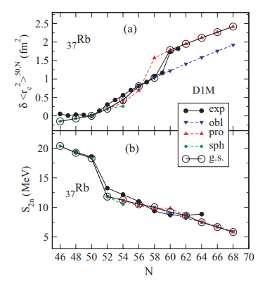
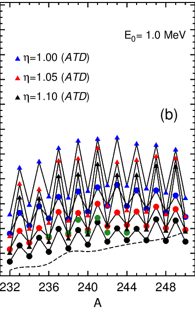
Figure 7: On the left hand side, the evolution of the nuclear radius and the two neutron separation energies is shown as a function of neutron number for several Rb ($Z=37$) odd mass isotopes. The evolution of the ground state deformation as $N$ increases is observed to go from spherical to oblate to prolate. The changes induced in the radius as a consequence of the shape changes are clearly observed. On the right hand side panel, the spontaneous fission half-live $t_{\mathrm{SF}}$ is plotted as a function of mass number A for several isotopes of Pu including even and odd number of neutrons. Experimental data is shown by green bullets, whereas experimental predictions are shown by bullets connected by lines. The different theoretical predictions correspond to different levels of enhancement of the pairing strength (blue, no enhancement; red, a 5% enhancement and purple, a 10 % enhancement. Figure adapted from Ref.[50]  [53, 51].

Calculations with full blocking using the Gogny force are scarce: there is the calculation of the properties of super-deformed rotational bands in ¹⁹¹Hg [115] or the recent proposal to do full blocking calculations but preserving axial symmetry [81]. The advantage of this proposal is that the $K$ quantum number is preserved and the assignment of the spin and parity of the ground state and excited band-heads is greatly facilitated. This approach has been used in a recent study of the properties of super-heavy nuclei [80]. In Fig 8 a comparison of the pairing gap $\Delta^{(3)}$ obtained with the EFA, full blocking and the simple Perturbative Quasiparticle approximation (see [81] for details) is presented for the Sn isotopic chain. From the plot we conclude that the time odd fields of the full blocking method have little impact on the gap $\Delta^{(3)}$ as the results obtained with this method are very similar to the ones of the EFA. Obviously, the perturbative approximation fails to quench pairing correlations as much as the other two approaches and therefore the pairing gap is significantly larger.

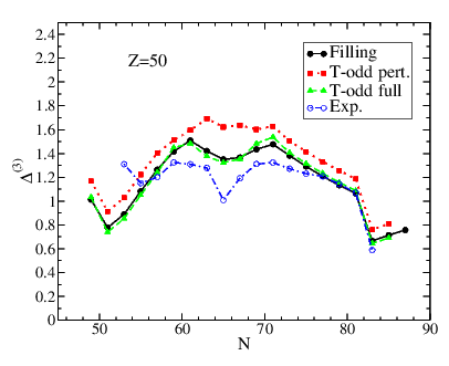
Figure 8: The pairing gap $\Delta^{(3)}$ is plotted as a function of neutron number for the tin isotopic chain for different approximations in the description of the unpaired odd neutron (EFA, full blocking and perturbative blocking). The theoretical results are compared to the experimental data. Figure adapted from Ref.[81].

Within the mean field HFB formalism it is also possible to study excited states that are given by multi-quasiparticle excitations. Multi-quasiparticle excited states can be considered perturbatively as the standard quasiparticle excitations built on top of a given HFB reference state [24]. The advantages of this approach are evident: the results are already available after a HFB calculation and the excited states are orthogonal by construction. On the other hand, self-consistency can play a very relevant role as multi-quasiparticle excitations tend to severely quench the pairing correlations present in the ground state. The drawbacks are multiple, first, as time reversal symmetry can be broken, the induced time odd fields (also present in the description of odd-A nuclei) have to be considered. Second, the iterative solution of the non linear problem is not easy to achieve even using standard gradient method techniques. Finally, the issue of orthogonality between the self-consistent multi-quasiparticle excitations and the ground state and among themselves becomes relevant. Some of these issues have been addressed in Ref. [82] where high $K$ isomers in ²⁵⁴No have been studied with both the D1S and D1M parametrizations of the Gogny force. The effects of self-consistency and the quenching of pairing correlations substantially reduce the excitation energy of the two-quasiparticle and four-quasiparticle isomers with respect to the naive sum of quasiparticle excitation energies built on top of the reference HFB ground state. In Fig 9 we have plotted the excitation energy of those high-$K$ isomers with known experimental excitation energies and compared them with our results. It is remarkable the good reproduction of the excitation energies given the rather universal scope of the Gogny force and its fitting protocol.

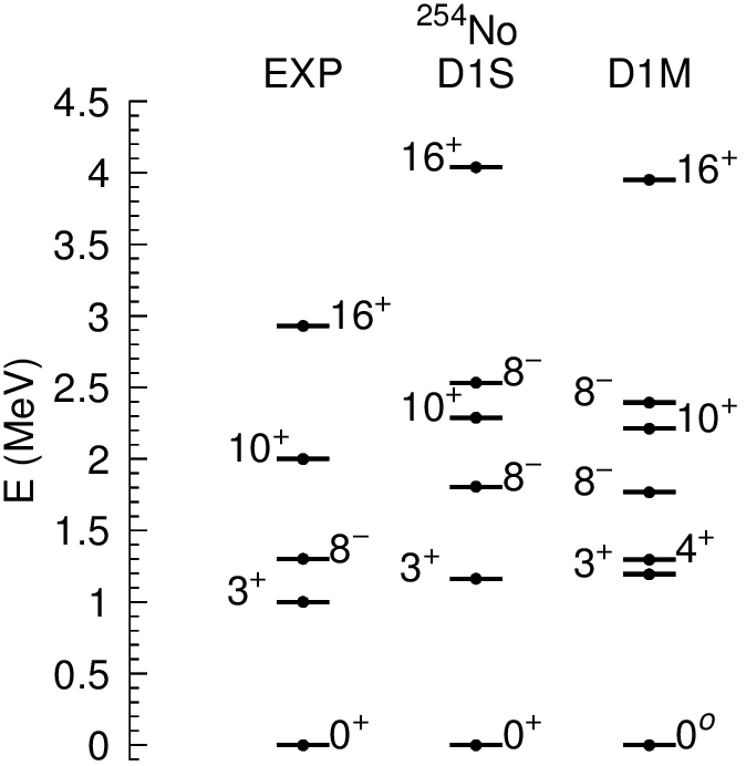
Figure 9: Excitation spectrum of high-K isomers computed self-consistently using the fully blocked HFB procedure with the D1S and D1M parametrizations of the Gogny force. On the left hand side of the plot the experimental spectrum is shown for comparison. Figure adapted from Ref.[82].

Another interesting field of application of the Gogny force is the study of nuclear matter properties at the mean field level. This studies allows to obtain, among other things, the Equation of State (EOS) of nuclear matter, of great relevance in astrophysical environments like the interior of neutron stars. In addition, the nuclear matter results can be compared to the ones of more sophisticated realistic interactions obtained with more elaborated many body techniques. In this respect, the evaluation of the Landau parameters of the different Gogny interactions has become a useful tool [116, 117]. The analysis of isovector properties like the symmetry energy or its slope give hints on the expected performance of the force in astrophysical environments or in very neutron rich scenarios [118]. Another interesting application of nuclear matter calculations is the study of the pairing gap and its comparison with realistic forces as analyzed in Refs [17, 16].

To end this section of applications of the HFB method, we will discuss the use of the finite temperature HFB (FT-HFB) formalism to describe the physics of highly excited nuclei using a grand-canonical ensemble formalism at fixed temperature T. Although the nucleus is a finite, isolated system, the ideas of quantum statistical mechanics have been used to describe situations where the intrinsic excitation energy of the nucleus is very high and therefore its wave function can be any among those in a bunch of excited states with a very large level density. Given the description of pairing correlations in terms of a mean field theory with no definite number of particles, the statistical ensemble to be used in nuclear physics is the grand canonical one, which allows both the exchange of energy and particles with a fictitious external reservoir. The quantity determining the density operator through a minimization principle is the free energy $F=H-TS$ that depends not only on the energy but also on the entropy $S$ and temperature $T$ of the system. The minimization of the free energy under the assumption that the density matrix is the exponential of a one-body operator and that the statistical trace has to be taken for all possible multi-quasiparticle excitations of a HFB ground state, leads to the FT-HFB equation. Its form is the same as in the zero temperature case and only the definition of the density and pairing tensor has to be replaced by the appropriate one

$$\mathcal{R}=W\left(\begin{array}[]{cc}f&0\\ 0&1-f\end{array}\right)W^{\dagger}$$ (59)

where the $f_{\mu}=1/(1+\exp(E_{\mu}/(K_{B}T))$ are the Fermi statistical occupation factors depending on the quasiparticle energies $E_{\mu}$ and the temperature. The FT-HFB equation has been solved with the Gogny force in order to study the phase transitions from super-fluid to normal-fluid systems with temperature as well as the transition from deformed to spherical driven also by temperature [31]. In the same reference, level densities are also evaluated using the FT-HFB formalism. Thermal fluctuations and their effect of washing out the abrupt phase transitions observed at the mean field level are analyzed in [119] in a variety of systems. Finally, the evolution of the fission barrier heights with temperature is studied in the case of ²⁴⁰Pu in Ref [120] where the decrease with temperature of the fission barrier heights is observed. As mentioned before, increasing the temperature means a quenching of pairing correlations that yield to an increase in the collective inertia [120].

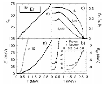
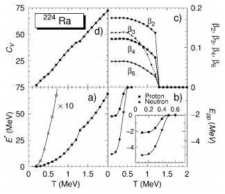
Figure 10: On the left hand side panels, the evolution with temperature ($T$ in MeV) of different quantities for the nucleus ¹⁶⁴Er. In panel a) the excitation energy $E^{*}$ in MeV, in panel b) the particle-particle energy, in panel c) the $\beta_{2}$, $\beta_{4}$ and $\beta_{6}$ deformation parameters and in panel d) the specific heat at constant volume $C_{V}$. In the right hand side panels, the same quantities are plotted for the octupole deformed nucleus ²²⁴Ra. The results were obtained with the Gogny D1S interaction. Figures taken from Ref.[31].

In Fig 10 the behavior with temperature of different quantities are shown for two different types of nuclei, the quadrupole deformed ¹⁶⁴Er and the quadrupole, octupole deformed ²²⁴Ra. The calculations are carried out with the Gogny D1S force in the context of FTHFB. In panels b) and c) in the two cases we observe (panel c)) the behavior of the deformation parameters $\beta_{\lambda}$ with temperature. A phase transition to an spherical regime is observed at $T=2.6$ MeV in the ¹⁶⁴Er case and at $T=1.3$ MeV in the octupole deformed ²²⁴Ra nucleus. Also, in panels b) a phase transition from a paired regime to an unpaired one at $T=0.6$ MeV. Both phase transitions produce a kink in the behavior of the specific heat at constant volume $C_{V}$ shown in panels d) and some discontinuity in the excitation energy $E^{*}$ of the system. The observed phase transitions are washed out when thermal fluctuations are considered [119].

In passing, let us mention that level densities can also be computed using combinatorial techniques and the uncorrelated quasiparticle spectrum obtained from a mean field calculation with the Gogny force [57]. The advantages and drawbacks of this method over the finite temperature formalism have to be still assessed but it is clear that any method based on the HFB ground state should have more difficulties to take into account the effects of finite temperature driven phase transitions like the transition to a normal fluid regime or from a deformed intrinsic state to a spherical one [31].

In Fig 11 the behavior of level densities as a function of the excitation energy are shown for the four nuclei considered in Ref [31], In the ¹⁶²Dy case it is compared with the experimental data. A rather good agreement with the experiment is observed when a phenomenological correction to take into account rotational bands is introduced.

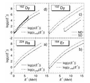
Figure 11: Logarithm of the level density $\rho(E^{*})$ plotted as a function of the excitation energy of the nucleus $E^{*}$ for four different nuclei ¹⁵²Dy, ¹⁶²Dy, ¹⁶⁴Er and ²²⁴Ra. The (full) dashed lines correspond to the calculation (without) with the rotational correction. Experimental data is also presented in the ¹⁶²Dy case. The calculations are carried out with the D1S force. Figures taken from Ref.[31].

3.2 Time dependent Hartree-Fock-Bogoliubov

The time dependent Hartree-Fock-Bogoliubov (TDHFB) method is the natural extension to treat dynamical aspects within the HFB theory. The generalized density matrix of HFB $\mathcal{R}$ is no longer static and its time evolution is governed by the TDHFB equation

$$i\hbar\frac{\partial\mathcal{R}}{\partial t}=[\mathcal{H},\mathcal{R}]$$ (60)

The TDHFB equation preserves the energy of the initial state (defined by $\mathcal{R}(t=0)$) and therefore cannot be used to describe tunneling through barriers, i.e. it is not possible to describe spontaneous fission. On the other hand, it can be used to study the time evolution of a wave packet confined in a potential well and in this way extract several properties of this kind of motion (elementary excitation energies, strengths, etc). The TDHFB method with the Gogny force has been recently implemented by Hashimoto [121] in a harmonic oscillator basis and preserving axial symmetry. The idea is to replace Eq (60) by the equivalent in terms of the Bogoliubov amplitudes $U$ and $V$

$$i\hbar\frac{\partial}{\partial t}\left(\begin{array}[]{c}\bar{U}\\ \bar{V}\end{array}\right)={}\mathcal{H}\left(\begin{array}[]{c}\bar{U}\\ \bar{V}\end{array}\right)$$ (61)

This is a non-linear system of equations because the HFB Hamiltonian $\mathcal{H}$ itself depends on $U$ and $V$ through its dependency in the density matrix $\rho=V^{*}V^{T}$ and the pairing tensor $\kappa=UV^{T}$. The solution to these coupled multidimensional non-linear differential equations is carried out using predictor-corrector techniques. The calculations focus on the isoscalar quadrupole and/or isovector dipole vibrations, in the linear (small amplitude) region, in some oxygen, neon, magnesium and titanium isotopes. The isoscalar quadrupole and isovector dipole strength functions are calculated from the expectation values of the isoscalar quadrupole and isovector dipole moments. This kind of calculations represent an alternative to the QRPA type of calculations mentioned in the next section. A more recent implementation, also preserving axial symmetry, replaces the harmonic oscillator basis along the $z$ direction by a Lagrange mesh. The reason for such replacement is to have far more flexibility in describing the time dependent density along the symmetry axis. This new implementation has been successfully applied to the description of head-on collisions in light systems [122].

4 Beyond mean field with the Gogny force: first applications

The mean-field approximation [84] allows the description of several basic nuclear properties all over the nuclear chart. However, in order to access the spectroscopy of atomic nuclei, one needs to go beyond the mean-field level. Several routes have emerged in recent years in order to afford such a task. On the one hand, the symmetry-projected Generator Coordinate Method (GCM) has already provided a wealth of results in different regions of the nuclear chart (see, for example, Refs. [94, 123, 124] and references therein). On the other hand, calculations are very demanding from a computational point of view, specially in the case of medium and heavy nuclei and/or when several collective coordinates should be included in the symmetry-projected GCM ansatz. This certainly limits, at least for the moment, the applicability of the approach from a computational point of view though progress is growing due to the new generation of computational facilities. All these methods along with some approximations to them will be discussed below in Sec 6. Another route is represented by the Quasiparticle Random Phase Approximation (QRPA) which can be viewed as a small-amplitude approximation to the GCM or the TDHFB methods [84]. A different alternative route is represented by fermion-to-boson mapping procedures described in Sec 4.2 below.

4.1 The QRPA

The quasiparticle random phase approximation (QRPA) is nothing but the small amplitude limit of arbitrary vibrations around the HFB equilibrium configuration [125, 84]. In the QRPA it is possible to study within the same framework not only collective excitations of isoscalar and isovector character, but also single particle excitations. The solution of the QRPA equation involves the construction and subsequent diagonalization of a huge matrix in the space of two quasiparticle excitations and therefore, applications with the Gogny force require a huge computational effort. Nevertheless, the advent of powerful computers allows for large scale calculations based on this method. QRPA calculations with Gogny interactions have been recently reviewed by Péru and Martini in Ref. [2]. Other QRPA implementations and applications of the most widely used energy density functionals like Skyrme [126, 127, 128, 129, 130, 131] and/or RMF [132, 133, 134] are out of the scope of the present review. Therefore, here we will only summarize the most important aspects and applications of the method, and update the list of most recent works done within the QRPA framework with Gogny interactions.

Derivation of QRPA equations and its formalism can be looked up in several textbooks (e.g. Ref. [84]). It is based on building two-quasiparticle excitations on top of a QRPA vacuum, $|\mathrm{QRPA}\rangle$, defined as:

$$\hat{\theta}_{\nu}|\mathrm{QRPA}\rangle=0;\hat{\theta}^{\dagger}_{\nu}=\frac{1}{2}\sum_{k<k^{\prime}}X^{\nu}_{kk^{\prime}}\beta^{\dagger}_{k}\beta^{\dagger}_{k^{\prime}}-Y^{\nu}_{kk^{\prime}}\beta_{k^{\prime}}\beta_{k}$$ (62)

where $(\beta^{\dagger}_{k},\beta_{k})$ are HFB quasiparticle creation and annihilation operators (see Eq. 6) and the amplitudes $(X^{\nu},Y^{\nu})$ are obtained from the QRPA equation given by [84]:

$$\left(\begin{array}[]{cc}A&B\\ B^{*}&A^{*}\end{array}\right)\left(\begin{array}[]{c}X^{\nu}\\ Y^{\nu}\end{array}\right)=E_{\nu}\left(\begin{array}[]{c}X^{\nu}\\ -Y^{\nu}\end{array}\right)$$ (69)

Here, $E_{\nu}$ are the excitation energies and the matrices $(A,B)$ are determined by the HFB state and the interaction through:

$$A_{kk^{\prime}ll^{\prime}} = \langle\mathrm{HFB}|\left[\beta_{k^{\prime}}\beta_{k},[\hat{H},\beta^{\dagger}_{l}\beta^{\dagger}_{l^{\prime}}]\right]|\mathrm{HFB}\rangle$$

$$B_{kk^{\prime}ll^{\prime}} = -\langle\mathrm{HFB}|\left[\beta_{k^{\prime}}\beta_{k},[\hat{H},\beta_{l}\beta_{l^{\prime}}]\right]|\mathrm{HFB}\rangle$$ (70)

In the implementations performed with Gogny forces, the same interaction is considered in the HFB and QRPA parts (normally neglecting two-body center-of-mass corrections and, in some cases, Coulomb exchange and pairing terms [2]).

Apart from the spectrum, $E_{\mu}$, the QRPA approach is widely used to study the response of the system to external fields. In the first implementations with the Gogny interaction, only spherical RPA (without pairing) were considered [135, 21, 136, 137, 61, 138, 139, 140]. In these works, nuclear compressibility, giant and pygmy resonances and excitations in closed-shell nuclei were studied. The inclusion of pairing (QRPA) and axial quadrupole deformation in this kind of calculations was performed for the first time by Péru et al. in Refs. [141, 142]. The assumption of axial and parity symmetry conservation allows for the classification of the QRPA states in terms of $K$ (the projection of the angular momentum $J$ along the symmetry axis) and $\pi$ (parity) quantum numbers, i.e., the QRPA states are given by [2]:

$$|\theta_{\nu},K\rangle=\hat{\theta}_{\nu,K}|0_{\mathrm{def}},(K=0)\rangle$$ (71)

where $|0_{\mathrm{def}}\rangle$ is the HFB ground state obtained with axially deformed calculations. The final evaluation of transition matrix elements of external fields given by the corresponding multipole operator, $\hat{Q}_{\lambda\mu}$, is obtained after projecting onto good angular momentum (see Sec 5, Eq 75) both the ground and the QRPA excited states:

$$|0^{+}_{\mathrm{g.s.}}\rangle = \frac{1}{8\pi^{2}}\int\mathcal{D}^{0*}_{00}(\Omega)\hat{R}(\Omega)|0_{\mathrm{def}}\rangle d\Omega$$

$$|JM(K)_{\nu}\rangle = \frac{2J+1}{8\pi^{2}}\int\mathcal{D}^{J*}_{MK}(\Omega)\hat{R}(\Omega)|\theta_{\nu},K\rangle d\Omega$$

Hence, the transition matrix elements are given by $\langle 0^{+}_{\mathrm{g.s.}}|\hat{Q}_{\lambda\mu}|JM(K)_{\nu}\rangle$ and the sum rules and moments by:

$$M_{k}\left(\hat{Q}_{\lambda\mu}\right)=\sum_{\nu}E_{\nu}^{k}|\langle 0^{+}_{\mathrm{g.s.}}|\hat{Q}_{\lambda\mu}|JM(K)_{\nu}\rangle|^{2}\\$$

For example, the energy weighted sum rule ($\mathrm{EWSM}(\hat{Q}_{\lambda\mu})$) is given by $M_{k=1}$ in the expression above.

Many calculations with the deformed QRPA method with Gogny interactions have been performed in the recent years, some of them with direct applications to nuclear astrophysics. For example, low-lying excitation energies, pygmy and giant resonances, electromagnetic multipole excitations and response functions, gamma-ray strength functions, reaction cross-sections, etc., in nuclei all along the nuclear chart have been studied and compared with experimental data where available [141, 142, 143, 144, 145, 146, 147, 2, 148, 149, 150, 151, 152, 153, 154]. In addition, Gamow-Teller response has been also computed with a proton-neutron QRPA method in Refs. [58, 155]. Finally, the role of continuum [139, 156], tensor interactions [157] and correlations beyond two-quasiparticle excitations [152] has been also analyzed recently. A thorough discussion of the performance of the method with several examples of its applications is found in the review of Péru and Martini and we refer the reader to Ref. [2] for further details.

4.2 IBM mapping

In order to extend the realm of the mean field to deal with spectroscopy in a simple way a novel method has been introduced in recent years [158]. It essentially maps the fermionic energy surfaces, obtained within the constrained mean-field approximation, onto the bosonic ones computed as the expectation value of a chosen Interacting Boson Model (IBM) [159] Hamiltonian in the boson coherent state. The fermion-to-boson mapping procedure determines the parameters of the chosen IBM Hamiltonian for each nuclear system and, therefore, no phenomenological adjustment of those parameters to the experimental data is required. It only relies on microscopic mean-field energy surfaces as the key input and, therefore, has the potential to provide predictions in those regions of the nuclear chart where experimental data are rather scarce or not even available as it is the case, for example, of exotic neutron-rich nuclei. The IBM Hamiltonian, obtained via the mapping procedure, is then diagonalized and the resulting wave functions are used to compute spectroscopic properties and transition rates. The fermion-to-boson mapping procedure has already allowed an accurate computationally economic and systematic description of basic properties in several regions of the nuclear chart.

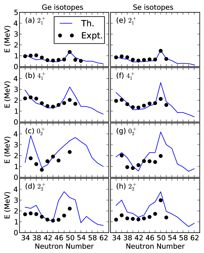
Figure 12: (Color online) The $2^{+}_{1}$, $4^{+}_{1}$, $0^{+}_{2}$ and $2^{+}_{2}$ excitation energies obtained in the diagonalization of the mapped IBM Hamiltonian are plotted as functions of the neutron number, for the Ge and Se nuclei, along with the available experimental data [160]. Taken from Ref. [161].

As an example of application we will consider a sample of results obtained for Ge and Se nuclei as they belong to one of the most challenging regions of the nuclear chart. Their structure and decay patterns have received considerable experimental [162, 163, 164, 165] and theoretical [166, 167, 168, 169, 170, 171, 172, 173, 174, 175, 176, 177, 178] attention in recent years. In particular, the shape transitions around the neutron sub-shell closure $N=40$ have already been studied in detail. Moreover, Ge and Se nuclei exhibit a pronounced competition between different configurations associated with a variety of intrinsic shapes, i.e., shape coexistence. The corresponding energy spectra display low-lying excited 0⁺ energy levels which could be linked to proton intruder excitations across the $Z=28$ shell gap.

The nuclei ^66-94Ge and ^68-96Se have been studied in Ref. [161]. The employed IBM model space consisted of collective nucleon pairs in the valence space with spins and parity $J^{\pi}$ = 0⁺ (monopole $S$ pair) and 2⁺ (quadrupole $D$ pair). They are associated with the $J^{\pi}$ = 0⁺ (s) and 2⁺ (d) bosons, respectively [179]. The microscopic input for the mapping, i.e., the mean-field energy surfaces as functions of the $\beta$ and $\gamma$ deformation parameters, have been obtained via Hartree-Fock-Bogoliubov (HFB) calculations with the parametrization D1M [42] of the Gogny interaction. Configuration mixing has been included in the corresponding (mapped) IBM calculations. To this end, the boson model space has been extended following a method, proposed by Duval and Barret [180], that incorporates the intruder configurations by introducing several independent IBM Hamiltonians. The intruder configurations correspond to proton $2p-2h$ excitations across the Z=28 shell gap and the different boson spaces are allowed to mix via certain mixing interaction. The criterion to include the configuration mixing for a given nucleus is that the second lowest-energy minimum in the mean-field energy surface is clear enough so as to constrain the corresponding (unperturbed) Hamiltonian for the intruder configuration. Therefore, configuration mixing has been taken into account for ^{66,70-74,90-94}Ge and ^68-76,90-96Se. All the required equations as well as the fitting procedure to obtain the parameters of the (mapped) IBM model can be found in Ref. [181]. Once the IBM parameters are determined for a given system, the Hamiltonian is diagonalized and the resulting wave functions are used to compute electromagnetic properties that could be considered as signatures of shape coexistence and/or shape transitions.

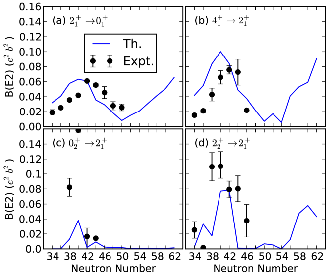
Figure 13: (Color online) The $B(E2;2^{+}_{1}\rightarrow 0^{+}_{1})$, $B(E2;4^{+}_{1}\rightarrow 2^{+}_{1})$, $B(E2;0^{+}_{2}\rightarrow 2^{+}_{1})$ and $B(E2;2^{+}_{2}\rightarrow 2^{+}_{1})$ transition probabilities obtained for Ge isotopes are plotted as functions of the neutron number. Experimental data have been taken from Ref. [160]. Taken from Ref. [161].

The excitation energies of the $2^{+}_{1}$, $4^{+}_{1}$, $0^{+}_{2}$ and $2^{+}_{2}$ states, obtained via the diagonalization of the mapped IBM Hamiltonian, are displayed in Fig. 12 as functions of the neutron number. They are compared with the available experimental data [160]. The calculations provide a reasonable agreement with the experimental systematics, especially for the yrast states. For both Ge and Se nuclei, the computed $E(2^{+}_{1})$ energies decrease as one approaches $N=40$. For the former, this is at variance with the experiment, a discrepancy that could be attributed to the $N=40$ neutron sub-shell closure not explicitly taken into account in the calculations [161]. The $E(2^{+}_{1})$ values display a pronounced peak at $N=50$. The experimental $E(4^{+}_{1})$ excitation energies [panels (b) and (f)] are overestimated around $N=50$. This could be linked to the limited IBM configuration space comprising only $s$ and $d$ bosons. Within this context, the inclusion of the $J=4^{+}$ ($G$) pair in the IBM model could improve the agreement with the experiment.

The predicted $E(0^{+}_{2})$ energies are plotted in panels (c) and (g). They display a pronounced decrease towards $N\approx 40$. This correlates well with the shape coexistence observed in the underlying Gogny-D1M energy surfaces around this neutron number [161]. The overestimation of the $E(0^{+}_{2})$ energy in the case of ⁶⁸Ge is due to the fact that a configuration mixing calculation has not been carried out in this case. For the considered neutron-rich nuclei, several examples of low-lying $0^{+}_{2}$ states are found beyond the $N=50$ shell closure [panels (c) and (g)]. As can be seen from panels (d) and (h), the calculations provide a reasonable description of the energies of the $2^{+}_{2}$ states which are, either interpreted as band-heads of the quasi-$\gamma$ bands or as members of the $0^{+}_{2}$ bands [161].

For both Ge and Se nuclei, the predicted excitation energies of the non-yrast states $E(0^{+}_{2})$ and $E(2^{+}_{2})$ are generally higher than the experimental ones especially for $46\leq N\leq 50$. This discrepancy is commonly observed in previous calculations for other mass regions (see, e.g., Ref. [182]) and could be, in most cases, attributed to the restricted model space of the IBM when the shell closure is approached.

The transition probabilities $B(E2;2^{+}_{1}\rightarrow 0^{+}_{1})$, $B(E2;4^{+}_{1}\rightarrow 2^{+}_{1})$, $B(E2;0^{+}_{2}\rightarrow 2^{+}_{1})$ and $B(E2;2^{+}_{2}\rightarrow 2^{+}_{1})$ are depicted in Fig. 13 for Ge isotopes. Similar results have been obtained for Se nuclei. The maximum $B(E2;2^{+}_{1}\rightarrow 0^{+}_{1})$ value is reached around $N=40$ where the deformation is the largest [161]. The agreement with the experimental data is fairly good. A similar trend is also found for the $B(E2;4^{+}_{1}\rightarrow 2^{+}_{1})$ transition rates shown in panel (b). The quantity $B(E2;0^{+}_{2}\rightarrow 2^{+}_{1})$, shown in panel (c), can be regarded as a measure of the mixing between different intrinsic configurations. The experimental $B(E2;0^{+}_{2}\rightarrow 2^{+}_{1})$ value is very large around $N=38$ or 40 where, a pronounced configuration mixing could be expected. Such a large value is not reproduced by the calculations. The origin of such a discrepancy between the theoretical predictions and the experiment could be associated to a weak mixing between the $2^{+}_{1}$ and $0^{+}_{2}$ states in the model. Some discrepancies between the predicted and experimental $B(E2;2^{+}_{2}\rightarrow 2^{+}_{1})$ values can be seen from panel (d). Nevertheless, the experimental trend, i.e., the $B(E2;2^{+}_{2}\rightarrow 2^{+}_{1})$ transition probability reaches its largest value at around $N=40$, being almost of the same order of magnitude as $B(E2;2^{+}_{1}\rightarrow 0^{+}_{1})$, is reproduced rather well by the calculations.

Several applications of the fermion-to-boson mapping procedure, with different levels of sophistication and intrinsic degrees of freedom, i.e., deformations, have already been discussed in the literature including the recent extensions of the model to describe the properties of odd-mass nuclear systems [181, 183, 184, 185, 186, 187, 188, 189, 182, 161, 190, 191, 192, 193, 187].

5 Beyond the mean field: symmetry restoration

The spontaneous breaking of symmetries by the nuclear mean field is one of its most salient features and it is a direct consequence of the properties of the nuclear interaction. An important aspect of the mean field, namely its non-linearity, is also responsible for the spontaneous breaking of symmetries. By breaking symmetries at the mean field level, a lot of correlations can be encoded into the wave function in a simple way. However, those broken symmetries have to be restored by considering appropriate linear combinations of mean field wave functions. In this way, the resulting wave functions recover the quantum number characteristic of the eigenstates of a symmetry invariant interaction/Hamiltonian [84, 194]. The mechanism of symmetry breaking along with the one of symmetry restoration leads to the fruitful concepts of ”intrinsic” and ”laboratory” frames of reference. The intrinsic frame corresponds to the symmetry breaking ”intrinsic” mean field state with its characteristic ”deformations” (like the prolate quadrupole deformation typical of many mid-shell nuclear ground states, or the diffuseness of the Fermi level typical of BCS wave functions present when the symmetry of the number of particles is broken). On the other hand the ”laboratory” system corresponds to the symmetry restored wave functions obtained as linear combinations of the intrinsic frame ones. The laboratory frame can be visualized as the frame of reference obtained after adding to the intrinsic frame the quantum fluctuations of ”orientation” in the appropriate variables . The impact of symmetry restoration in the absolute value of the binding energy of a typical nucleus is not too high, of a few per thousand. This is also the case if the observable is associated to a scalar quantity (i.e. invariant under the symmetry operation). However, the values of the electromagnetic transition strengths involving overlaps of tensor operators are very sensitive to the effects of symmetry restoration. For instance, to reproduce the selection rules typical of those strengths, the wave functions involved must have the proper quantum numbers, a property that is only obtained after symmetry restoration.

In this section, we will develop the main ideas of symmetry restoration and apply them to the study of the most relevant cases in nuclear physics: (a) reflection symmetry (b) particle number, (c) rotational symmetry and (d) translational invariance. Prominent examples of the application of such symmetry restorations will be briefly discussed. We will also discuss the approximate evaluation of projected quantities under the assumptions of strong deformation of the intrinsic state not only because this is a cheap, and in many cases, sufficient way to incorporate the effects of symmetry restoration but also because it is the basis of the rotational model of Bohr and Mottelson [195] that has proven to be so successful in explaining lots of phenomenology in nuclear structure.

5.1 General principles

The starting point of symmetry restoration is, obviously, the existence of a spontaneous symmetry breaking intrinsic mean field wave function. This wave function is obtained from some interaction or EDF by solving the non-linear HF or HFB equations. The symmetry restored (or projected) wave functions are obtained by considering appropriate linear combinations of the ”rotated” intrinsic states (that is, the intrinsic state after applying to it a member of the symmetry group). With these wave functions (there are as many as the number of irreducible representations of the underlying symmetry group) we can compute physical observables like the projected energy, radius, electromagnetic moments, etc. This procedure is known under the name of projection after variation (PAV) because the ”intrinsic wave function” is obtained by minimizing the intrinsic energy, and therefore knows nothing about its subsequent projection [196, 197, 84]. At this point one might wonder about the usefulness of considering the projected energies (one for each irrep of the symmetry group) as the quantities to apply the variational principle in order to obtain the ”intrinsic” states. The most immediate consequence of this procedure is that different intrinsic states are obtained for each projected energy considered. Another consequence is that the projected wave function is richer than the set of intrinsic ones and therefore the procedure is variationally effective, that is, a lower energy than the intrinsic one is always going to be obtained at least for one of the projected energies. This procedure is known as variation after projection (VAP) [198, 199, 200, 84] and is formally superior to PAV as shown in many examples and test studies in simple models. The main disadvantage of VAP over PAV is that the projected energies are far more involved to compute than the intrinsic (mean field) one. Not to mention also the fact that for each quantum number a minimization has to be carried out.

5.1.1 Symmetry restoration, general group theory arguments

The procedure to restore symmetries is deeply rooted in the underlying group structure of the symmetry operations [84, 194]. The set of symmetry operations is endowed with the mathematical structure of a group. For instance, spatial rotations are associated to the continuous Lie group $SU(2)$, reflection symmetry is associated to a discrete, idempotent group made of two elements, the identity and the parity operator $\Pi$ satisfying $\Pi^{2}=\mathbb{I}$. The quantum numbers of the restored symmetries are the labels of the irreducible representations (irreps) of the group, or, in the case of Lie groups of the irreps of the associated algebra. For instance, in the case of $SU(2)$ the corresponding algebra $su(2)$ is composed of the angular momentum operators $J_{x}$, $J_{y}$ and $J_{z}$. The irreps of the angular momentum operators correspond to the eigenstates of $J^{2}=J_{x}^{2}+J_{y}^{2}+J_{z}^{2}$ and $J_{z}$ and are labeled by the typical $J$ and $M$ quantum numbers. The basis states of the irreps are the eigenstates $|JM\rangle$. The subspace spanned by each irrep is invariant under the operator realizing the symmetry. For instance, consider the rotation operator which can be expressed in terms of the Euler angles $\Omega=(\alpha,\beta,\gamma)$

$$\hat{R}(\Omega)=e^{-i/\hbar\alpha J_{z}}e^{-i/\hbar\beta J_{y}}e^{-i/\hbar\gamma J_{z}}$$ (73)

The matrix element of the rotation operator between basis states of two different irreps gives

$$\langle J^{\prime}M^{\prime}|\hat{R}(\Omega)|JM\rangle=\delta_{JJ^{\prime}}\mathcal{D}^{J}_{M^{\prime}M}(\Omega)$$ (74)

where the Wigner rotation matrix $\mathcal{D}^{J}_{M^{\prime}M}(\Omega)$ has been introduced. The $\delta_{JJ^{\prime}}$ in the above expression shows that the subspace spanned by $|JM\rangle$ is indeed invariant under the symmetry operator $\hat{R}(\Omega)$. By taking linear combinations of the rotation operator with the Wigner functions and using the appropriate integration measure (de Haar measure) we end up with the projection operator

$$\hat{P}^{J}_{MK}=\frac{2J+1}{8\pi^{2}}\int d\Omega\mathcal{D}^{J\,*}_{MK}(\Omega)\hat{R}(\Omega)$$ (75)

which is labeled with the indices of the irreps of the corresponding group. In the $SU(2)$ case it has the properties

$$P^{J}_{MK}P^{J}_{M^{\prime}K^{\prime}}=\delta_{JJ^{\prime}}\delta_{M^{\prime}K}\hat{P}^{J}_{MK^{\prime}}$$ (76)

and

$$\left(\hat{P}^{J}_{MK}\right)^{\dagger}=\hat{P}^{J}_{KM}$$ (77)

Due to the special structure of the projector, the action of the symmetry operator on the left (or the right) of the projector leads to a linear combination of the same projector with weights which are nothing but the representation of the symmetry operator in the linear space of the irreps

$$\hat{R}(\Omega)\hat{P}^{J}_{MK}=\sum_{K^{\prime}}\mathcal{D}^{J}_{MK^{\prime}}(\Omega)\hat{P}^{J}_{K^{\prime}M}$$ (78)

which suggests the following form of the projector

$$\hat{P}^{J}_{MK}=\sum_{\alpha}|JM\alpha\rangle\langle JM\alpha|$$ (79)

where $\alpha$ represents an additional set of quantum numbers required to fully characterize the quantum states.

5.1.2 Symmetry breaking as generator of symmetry bands (rotational, parity, etc)

For each intrinsic (deformed) state $|\Phi\rangle$ we can generate a whole set of states with the appropriate symmetry quantum numbers. Using again the angular momentum as an example, for each deformed states $|\Phi\rangle$ we can generate infinite (in principle) states

$$|\Psi_{JM}\rangle=\sum_{K}g_{K}^{J}\hat{P}^{J}_{MK}|\Phi\rangle$$ (80)

eigenstates of $\hat{J}^{2}$ and $\hat{J}_{z}$ labeled by the $J$ and $M$ quantum numbers. We have generated, in this way, a ”rotational band” which is nothing but the set of $|\Psi_{JM}\rangle$ states. The physical properties of those states will strongly depend on the degree of deformation of the intrinsic state $|\Phi\rangle$ as discussed below. We can compute the energy for each member of the band

$$E^{J}=\frac{\langle\Psi_{JM}|\hat{H}|\Psi_{JM}\rangle}{\langle\Psi_{JM}|\Psi_{JM}\rangle}$$ (81)

which is independent of $M$ as a consequence of the scalar nature of $\hat{H}$. The dependence of $E^{J}$ with $J$ depends on the structure of the intrinsic state $|\Phi\rangle$ although it is possible to extract general properties in the case in which the intrinsic state is strongly deformed. As it will be shown below, in the strong deformation limit the energy is given by

$$E^{J}=\langle\Phi|\hat{H}|\Phi\rangle-\frac{\langle\Delta\vec{J}^{2}\rangle}{2\mathcal{J}_{\mathrm{Y}}}+\frac{\hbar^{2}J(J+1)}{2\mathcal{J}_{\mathrm{Y}}}$$ (82)

that is the characteristic expression for the energy of a rotational band with the characteristic $J(J+1)$ growing of the energy with angular momentum. In this expression $\mathcal{J}_{\mathrm{Y}}$ is the Yoccoz moment of inertia defined, for instance in [196, 197, 201, 84]. Along the same line of reasoning, the breaking of reflection symmetry followed by parity restoration requires a projector which is proportional to $\mathbb{I}+\pi\hat{\Pi}$ with the parity quantum number $\pi=\pm 1$. In the strong deformation limit $\langle\hat{\Pi}\rangle\rightarrow 0$ the projected energy $E^{\pi}=(\langle\hat{H}\rangle+\pi\langle\hat{H}\hat{\Pi}\rangle)/(1+\pi\langle\hat{\Pi}\rangle$ is degenerate leading to a ”band” composed of two elements which are degenerated in energy.

Breaking of several symmetries at the same time is also possible and its restoration leads to an ”admixture” of bands, like the alternating parity rotational bands characteristic of octupole deformation at high spins. In this case, rotational and reflection symmetries are broken at the same time.

5.1.3 Evaluation of overlaps: generalized Wick theorem and Pfaffian

The evaluation of the ”projected” quantities, like energies or transition strengths, requires the evaluation of an integral over the parameters of the symmetry group of the corresponding operator’s overlaps. To be more specific, and using again the example of $SU(2)$ we need to evaluate integrals involving quantities like

$$H(\Omega) = \langle\Phi|\hat{H}\hat{R}(\Omega)|\Phi\rangle$$ (83)

$${}N(\Omega) = \langle\Phi|\hat{R}(\Omega)|\Phi\rangle$$

which are overlaps of the corresponding operators between the intrinsic HFB wave function $|\Phi\rangle$ and the ”rotated” one $\hat{R}(\Omega)|\Phi\rangle$. Fortunately, all the symmetry groups considered in nuclear physics are either discrete or compact Lie groups. In the later case, the symmetry operators are written in terms of exponentials of the corresponding Lie algebra that is represented in Fock space as linear combinations of one body operators ($J_{i}$, $P_{i}$, etc). As a consequence, we can use Thouless theorem to show that $\hat{R}(\Omega)|\Phi\rangle$ is again a HFB wave function and therefore, we are dealing with overlaps of operators between different HFB wave functions (the arguments below can be extended straightforwardly to the case where $|\Phi\rangle$ is replaced by a more general HFB wave function $|\Phi^{\prime}\rangle$ ). The evaluation of the overlaps is carried out using the generalized Wick theorem and the overlap formula as discussed in Appendix C. The expressions derived in the Appendix are obtained under the assumption that the original single particle basis and the rotated one span the same subspace of the total Hilbert space. This is not the case if the basis breaks the symmetry under consideration. Typical examples are the use of deformed harmonic oscillator basis in the case of rotations or basis not translational invariant in the case of Galilei invariance restoration. This difficulty leads to either the use of symmetry restricted basis (for instance, HO basis with equal oscillator lengths along all possible spatial directions - see below) or a careful evaluation of the impact of truncation errors as is the case in the restoration of Galilei invariance (see below).

The overlaps can be evaluated in terms of linear combinations of products of contractions with the use of the generalized Wick’s theorem. For instance, the ratio $h(\Omega)=H(\Omega)/N(\Omega)$ is given by

$$h(\Omega)=\sum_{ab}t_{ab}\rho_{ba}(\Omega)+\frac{1}{4}\sum_{abcd}\bar{\nu}_{abcd}[\rho_{db}(\Omega)\rho_{ca}(\Omega)-\rho_{da}(\Omega)\rho_{cb}(\Omega){}+\kappa_{dc}(\Omega)\bar{\kappa}_{ba}(\Omega)]$$ (84)

where the ”elemental” contractions are given by quantities that resemble very much the standard HFB density matrix and pairing tensor

$$\rho_{db}(\Omega) = \frac{\langle\Phi|c^{\dagger}_{b}c_{d}\hat{R}(\Omega)|\Phi\rangle}{\langle\Phi|\hat{R}(\Omega)|\Phi\rangle}$$ (85)

$$\kappa_{dc}(\Omega) = \frac{\langle\Phi|c_{c}c_{d}\hat{R}(\Omega)|\Phi\rangle}{\langle\Phi|\hat{R}(\Omega)|\Phi\rangle}$$ (86)

$$\bar{\kappa}_{ba}(\Omega) = \frac{\langle\Phi|c^{\dagger}_{a}c^{\dagger}_{b}\hat{R}(\Omega)|\Phi\rangle}{\langle\Phi|\hat{R}(\Omega)|\Phi\rangle}$$ (87)

Once the quantity $h(\Omega)$ is obtained, the evaluation of $H(\Omega)$ is straightforward (however, see below for the case where $N(\Omega)=0$ for some $\Omega$). The remaining term, $N(\Omega)$ is given in terms of determinants or Pfaffians of the appropriate matrices (see Appendix C).

5.1.4 Difficulties associated with the Pauli exclusion principle and self-energies

In the implementation of symmetry restoration and configuration mixing, to be discussed below, one has to face technical difficulties associated with the evaluation of the overlaps in Eq 84 and having to do with the vanishing of the overlap between the two HFB states. Let us define the overlap

$$h(q,q^{\prime})=\frac{\langle\varphi_{q}|\hat{H}|\varphi_{q^{\prime}}\rangle}{\langle\varphi_{q}|\varphi_{q^{\prime}}\rangle}$$ (88)

where $|\varphi_{q}\rangle$ is a HFB wave function parametrized in terms of the labels denoted collectively as $q$. The generalized Wick’s theorem allows to express the above overlap in terms of the contractions

$$\rho_{db}(q,q^{\prime}) = \frac{\langle\varphi_{q}|c^{\dagger}_{b}c_{d}|\varphi_{q^{\prime}}\rangle}{\langle\varphi_{q}|\varphi_{q^{\prime}}\rangle}$$ (89)

$$\kappa_{dc}(q,q^{\prime}) = \frac{\langle\varphi_{q}|c_{c}c_{d}|\varphi_{q^{\prime}}\rangle}{\langle\varphi_{q}|\varphi_{q^{\prime}}\rangle}$$ (90)

$$\bar{\kappa}_{ba}(q,q^{\prime}) = \frac{\langle\varphi_{q}|c^{\dagger}_{a}c^{\dagger}_{b}|\varphi_{q^{\prime}}\rangle}{\langle\varphi_{q}|\varphi_{q^{\prime}}\rangle}$$ (91)

In general, the quantities $\langle\varphi_{q}|c^{\dagger}_{b}c_{d}|\varphi_{q^{\prime}}\rangle$, $\langle\varphi_{q}|c_{c}c_{d}|\varphi_{q^{\prime}}\rangle$ or $\langle\varphi_{q}|c^{\dagger}_{a}c^{\dagger}_{b}|\varphi_{q^{\prime}}\rangle$ are, by construction, finite. In the case when $\langle\varphi_{q}|\varphi_{q^{\prime}}\rangle$ is zero, this implies that $\rho_{db}(q,q^{\prime})$, $\kappa_{dc}(q,q^{\prime})$ and $\bar{\kappa}_{ba}(q,q^{\prime})$ must be divergent. If the overlap goes to zero like a small parameter $\epsilon$, then the contractions must diverge like $1/\epsilon$. As a consequence, the overlap of one body operators $\langle\varphi_{q}|\hat{T}|\varphi_{q^{\prime}}\rangle$ is manifestly finite as it only involves the contraction $\rho_{db}(q,q^{\prime})$ times the overlap $\langle\varphi_{q}|\varphi_{q^{\prime}}\rangle$. The difficulties arise in the evaluation of two (or higher order) operators as in this case we have products of two contractions that behave like $1/\epsilon^{2}$. A simplistic analysis would lead to the conclusion that $\langle\varphi_{q}|\hat{H}|\varphi_{q^{\prime}}\rangle$ must diverge when $\langle\varphi_{q}|\varphi_{q^{\prime}}\rangle$ goes to zero. However, a more careful analysis reveals that, due to the properties of the fermion creation and annihilation operator algebra (that lead to the Pauli exclusion principle), the sum of the products of two contractions

$$\rho_{db}(q,q^{\prime})\rho_{ac}(q,q^{\prime})-\rho_{da}(q,q^{\prime})\rho_{bc}(q,q^{\prime})+\kappa_{dc}(q,q^{\prime})\bar{\kappa}_{ba}(q,q^{\prime})$$ (92)

cancel one of the inverse powers of $\epsilon$ as to render $\langle\varphi_{q}|\hat{H}|\varphi_{q^{\prime}}\rangle$ finite. This discussion might look a bit of an academic one as it is very unlikely that given a discrete set of $q$ values one is going to find a zero overlap. However, the important point is that if the overlap is small because it is close to a zero, then the contractions are going to take very large values that still need large cancellations in order to get the proper value of the overlap $\langle\varphi_{q}|\hat{H}|\varphi_{q^{\prime}}\rangle$. Very often, both in the evaluation of the energy or the Hamiltonian overlap several contributions ,like Coulomb exchange or Coulomb anti-pairing are neglected. This means that not all the terms in Eq. 92 are considered and therefore in the event of being close to a zero of the overlap the cancellation mentioned above does not take place and the overlap might become unnaturally and unphysically large. This also happens if two different interactions are used in the ph and pp channels as only the first two terms in the sum of Eq. 92 are considered in the ph channel and the last one in the pp channel. This problem is dubbed in the literature as the ”self-energy” and/or ”self-pairing” problem [202]. The reason for that name is that it shares the same origin with another typical problem encountered in the evaluation of two body operators and consequence of neglecting the exchange or pairing terms: the mean value of the Hamiltonian computed with a mean field wave function corresponding to just one particle is different from zero in spite of not having other particle to interact with. In the case of the Gogny force calculations, where the pairing field is obtained from the same interaction used in the ph channel, the best solution is to fully consider all the neglected terms, namely the Coulomb exchange, Coulomb anti-pairing and spin-orbit pairing fields. Unfortunately, considering the Coulomb contributions increase by almost and order of magnitude the computational requirements to compute mean values of overlaps. Another, more important, consequence is that all the Gogny forces incepted so far do not consider exact Coulomb exchange and Coulomb anti-pairing and therefore their parameters are not fully adapted to their consideration. The ”self-energy” problem is ubiquitous in Particle number projection calculations and seems to be less dangerous in applications of the generator coordinate method without projection. This issue has been discussed at length in the literature [203, 92, 204, 202, 3] and the reader is referred to the mentioned literature for further details.

5.1.5 Difficulties associated with non-integer powers of the density

Density dependent forces, like Gogny, are state dependent, i.e. the interaction depends upon the matter density of the corresponding state. Nevertheless, they are unambiguously defined in the calculation of the mean value of the energy as the matter density to be used in the density dependent part of the interaction is just the mean value of the density operator. This is not the case, however, in the calculation of overlaps of the Hamiltonian between different HFB states that is required, for instance, in the implementation of symmetry restoration or large amplitude motion discussed below. In those situations, a prescription for the density dependent part of the interaction is required. The most obvious one is to replace the density in the density dependent part of the interaction by the mixed density [205]

$$\rho_{q,q^{\prime}}=\frac{\langle\varphi(q)|\hat{\rho}(\vec{R})|\varphi(q^{\prime})\rangle}{\langle\varphi(q)|\varphi(q^{\prime})\rangle}$$ (93)

which is the overlap of the matter density operator $\hat{\rho}(\vec{R})=\sum_{i=1}^{A}\delta(\vec{r}_{i}-\vec{R})$ between the corresponding HFB sates $|\varphi(q)\rangle$ and $|\varphi(q^{\prime})\rangle$. This prescription fulfills a series of requirements like leading to overlaps of scalar operators invariant under symmetry operations or other properties essential to ensure that observables are real quantities [124, 206]. The main objection to this prescription is that, in the general case, the overlap density is a complex quantity that has to be raised to a non integer power $\alpha$, as it is the case in all of the popular phenomenological effective interactions of the Gogny or Skyrme type. Raising complex numbers $z=|z|e^{i\varphi}$ to non-integer powers is a delicate operation that leads to multi-valued solutions (in general infinite ones) of the form $|z|^{\alpha}e^{i\alpha\varphi+2\pi\alpha in}$ where $n$ represent all positive integers $n=0,1,2,\ldots$. Those multi-valued powers (or roots) have to be located in Riemann sheets and special attention has to be paid to continuity issues in going from one Riemann sheet to another. If those discontinuities are not treated adequately they might lead to jumps in the integrals leading to the projected energy. This issue has been discussed in detail in Refs [204, 207] but so far no evident general solution to this problem seems to exist. However, wise choices of phases lead to very reasonable results which seem to be free from the artifacts of discontinuous integrands. A possible solution to this problem would be to use symmetry invariant densities which are given by mean values with projected wave functions or linear combinations of mean values evaluated with rotated intrinsic quantities. In any of the two possibilities, they are real quantities and therefore free from the uncertainties in the determination of the non-integer power. However, it has been shown that this prescription is inconsistent with the general philosophy of the density dependent term in the case of spatial symmetries like parity or angular momentum [208] leading to catastrophic results. Nevertheless, this prescription, when used only in the particle number restoration leads to reasonable results as it will be shown below.

5.2 Parity Projection

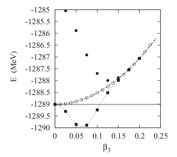
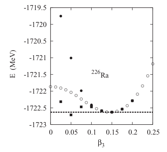
Figure 14: HFB (open circles), positive parity (full squares) and negative parity (bullets) energies as a function of the $\beta_{3}$ deformation parameter for the ¹⁵⁸Gd (left) and ²²⁶Ra (right) nuclei. The Gogny D1S parameterization is used. Figure adapted from Ref. [29].

Parity projection is the simplest possible example of symmetry restoration because the symmetry operators belong to a discrete set with only two elements, the identity $\mathbb{I}$ and the parity operator $\hat{\Pi}$. As the parity operator satisfies $\hat{\Pi}^{2}=\mathbb{I}$ the parity quantum number can only take two values $\pi=\pm 1$. The expression of the projection operator $\hat{P}_{\pi}$ and the projected energy are specially simple in this case

$$\hat{P}_{\pi}=\frac{1}{2}(\mathbb{I}+\pi\hat{\Pi})$$ (94)

and

$$E_{\pi}=\frac{\langle\hat{H}\rangle+\pi\langle\hat{H}\hat{\Pi}\rangle}{1+\pi\langle\hat{\Pi}\rangle}$$ (95)

When the degree of symmetry breaking of the intrinsic wave function is large $\langle\hat{\Pi}\rangle\approx 0$, the Hamiltonian overlap $\langle\hat{H}\hat{\Pi}\rangle$ can be neglected with respect to $\langle\hat{H}\rangle$ and therefore we obtain a degenerate energy for both parities (a parity doublet) that corresponds to the intrinsic energy. The parity doublet is nothing but the ”band” generated by the restoration of the parity symmetry of an intrinsic state which is strongly deformed.

Parity (or reflection symmetry) breaking is associated with the lowest relevant negative parity multipole moment of the mass distribution, namely the octupole moment $Q_{3\mu}$. Octupole deformation of the ground state of atomic nuclei is not as common as quadrupole deformation and its presence requires that proton and neutron numbers are close or equal to specific values such that the Fermi level is close to opposite parity orbitals with $\Delta l=3$. Those specific numbers are $N=40,56,88,136$, etc. Nuclei with proton and neutron number close to them correspond to paradigmatic octupole deformed systems like ¹⁴⁴Ba [101, 100] or ²²⁴Ra [99]. When the nucleus is octupole deformed, the parity splitting $\Delta E_{\pm}=E_{\pi=+1}-E_{\pi=-1}$ is very small and parity doublets appear characterized by strong $B(E3)$ transition probabilities. This description is not very accurate as fluctuations in the octupole degree of freedom (taken into consideration, for instance, with the GCM, see Sec 6) modify quantitatively the picture. Octupole effects are, however, pervasive and appear all over the periodic table when parity projection is considered in the VAP or restricted variation after projection (RVAP) framework. In the latter case, we consider a set of HFB configurations constrained on the value of the octupole moment $Q_{30}$ and compute the projected energies $E_{\pi}(Q_{30})$. The corresponding minima for the positive and negative parity curves are in general different (they only coincide in octupole deformed nuclei) leading to two intrinsic states associated to the two possible parities. In this way, it is possible to compute the parity splitting $\Delta E$ for all nuclei and the corresponding $B(E3)$ strengths. In addition, the absolute minimum of the two curves very often lies at an excitation energy lower than the one of the HFB minimum being the energy gain the octupole correlation energy. This procedure has been carried out with the D1S, D1N and D1M variants of the Gogny force in Refs [29, 37] for a large set of even-even nuclei spanning a wide subset of the nuclide chart. In Fig 14 an example of the RVAP procedure taken from [29] is shown for an octupole soft nucleus ¹⁵⁸Gd and for a well deformed one ²²⁴Ra. Both parity projected energies are plotted as a function of the $\beta_{3}$ deformation parameter, along with the HFB energy. In the octupole soft case we observe two well differentiated minima, one for positive parity the other for negative parity, at different excitation energies. On the other hand, for the nucleus ²²⁴ Ra the three minima (HFB, positive parity and negative parity) are located at the same $\beta_{3}$ value and have the same energy. Therefore, the parity splitting between positive and negative parity states is essentially zero.

Another useful application of parity projection is to show some of the difficulties associated to symmetry restoration in the presence of density dependent forces like Gogny: in Ref [208] it was shown that the use of the symmetry restored density in the density dependent term of the Gogny interaction results in catastrophic consequences. The only consistent density dependent prescription in the restoration of spatial symmetries seems to be the ”mixed density” (see above, Sec 5.1.5). This result can be straightforwardly extended to any of the flavors of the Skyrme EDF.

Parity projection has also been applied with intrinsic HFB cranking states to describe the stabilization of octupole deformation with increasing angular momentum and the corresponding emergence of ”alternating parity rotational bands” [109, 110].

5.3 Particle number projection (PNP)

As it was mentioned above, pairing correlations are allowed to be present in the mean-field approximation through the Bogoliubov transformation. This implies that the HFB wave functions are not (in general) eigenstates of the proton and neutron number operators. Such a symmetry breaking mechanism is very useful to explore some relevant terms of the nuclear interaction with relatively simple many-body wave functions. However, it is obvious that the physical nuclear states of a specific nucleus must have a definite number of protons and neutrons, i.e., they have to be eigenstates of those operators. Additionally, in cases where the single-particle level density around the Fermi level is small, the HFB approach itself is unable to capture pairing correlations at all and the method collapses into a pure HF state. These and other drawbacks can be corrected by restoring the particle-number symmetry of the nuclear system. The restoration relies on projection techniques that produce many-body states as linear combinations of mean-field wave-functions with the coefficients dictated by the symmetry group U(1) (see discussion in Sec 5.1.1). Hence, the particle-number projected (PNP) wave functions are defined as [84]:

$$|NZ\rangle=\hat{P}^{N}\hat{P}^{Z}|\Phi\rangle$$ (96)

where $|\Phi\rangle$ is a HFB state and $\hat{P}^{N(Z)}$ is the projection operator onto a good number of neutrons (protons):

$$\hat{P}^{N}=\frac{1}{2\pi}\int_{0}^{2\pi}e^{i\varphi(\hat{N}-N)}d\varphi$$ (97)

Once the PNP wave functions are defined, the projection itself can be performed before or after the variational procedure [84]. In both cases the variational space is made of HFB (intrinsic) states and the difference comes from the energy functional that is minimized.

In the projection after variation (PAV) approach the HFB energy is minimized first and the resulting intrinsic wave function is projected afterwards:

$$\left.\delta E^{{}^{\prime}\mathrm{HFB}}\left[|\Phi\rangle\right]\right|_{|\Phi\rangle=|\mathrm{HFB}\rangle}=0\Rightarrow$$

$$\Rightarrow|NZ\rangle_{\mathrm{PN-PAV}}=\hat{P}^{N}\hat{P}^{Z}|\mathrm{HFB}\rangle$$ (98)

where $E^{{}^{\prime}\mathrm{HFB}}\left[|\Phi\rangle\right]$ is the energy density functional (EDF) computed within the HFB approximation:

$$E^{{}^{\prime}\mathrm{HFB}}\left[|\Phi\rangle\right]=\langle\hat{H}\rangle+\varepsilon^{\mathrm{DD}}\left[|\Phi\rangle\right]-\lambda_{Z}\langle\hat{Z}\rangle-\lambda_{N}\langle\hat{N}\rangle$$ (99)

Here $|\rangle\equiv|\Phi\rangle$, $\lambda_{Z(N)}$ are the Lagrange multipliers to ensure the correct mean value of the number of protons (neutrons) in the intrinsic wave function, and $\hat{H}$ and $\varepsilon^{\mathrm{DD}}\left[|\Phi\rangle\right]$ are the Hamiltonian piece and the explicit density-dependent part of the nuclear interaction, respectively.

This method is computationally cheap since it only requires one PN projection at the end of the process. However, the collapse of the pairing correlations in the HFB approach in weak pairing regimes remains unsolved using the PAV method. In these situations the HFB states are pure HF wave functions that do not break the particle number symmetry and PN-PAV does not have any effect.

The natural way to improve the PN-PAV method is the so-called variation after projection (PN-VAP) technique where the projected energy instead of the HFB energy is minimized.

$$\left.\delta E^{\mathrm{PNP}}\left[|\Phi\rangle\right]\right|_{|\Phi\rangle=|\mathrm{PN-VAP}\rangle}=0\Rightarrow$$

$$\Rightarrow|NZ\rangle_{\mathrm{PN-VAP}}=\hat{P}^{N}\hat{P}^{Z}|\mathrm{PN-VAP}\rangle$$ (100)

In this case $E^{\mathrm{PNP}}\left[|\Phi\rangle\right]$ is the EDF that includes the particle number restoration:

$$E^{\mathrm{PNP}}\left[|\Phi\rangle\right]=\frac{\langle\hat{H}\hat{P}^{N}\hat{P}^{Z}\rangle}{\langle\hat{P}^{N}\hat{P}^{Z}\rangle}+\varepsilon^{\mathrm{DD,PNP}}\left[|\Phi\rangle\right]$$ (101)

It is important to notice that the EDF coming from the explicit density-dependent part of the interaction, $\varepsilon^{\mathrm{DD,PNP}}\left[|\Phi\rangle\right]$, requires a more detailed explanation that will be given below (see also Secs 5.1.4 and 5.1.5).

The amount of pairing correlations included by using this method is larger than the PN-PAV and, moreover, the collapse of the pairing correlations is avoided. The problem is the higher computational cost of the PN-VAP method since the symmetry restoration is performed in every step of the resolution of the variational equations. Nevertheless, this is not a serious limitation of the method with the present computing capabilities.

Both PN-PAV and PN-VAP approaches are exact projections onto good number of protons and neutrons. However, the first implementations of the PNP with Gogny interactions were made in the self-consistent second-order Kamlah (SCK2) [105] and Lipkin-Nogami (LN) [209, 210] approximations, being the latter an approximation itself to the former [211, 97, 108, 212] (see Sec 5.6 below). One of the first applications of these approximate methods was the study of deformed and super-deformed bands at high spin in rare earth nuclei and in Hg isotopes around $A=190$ [211, 97, 108, 212]. In Fig. 15 we show an example of the performance of HFB, LN and SCK2 approaches in cranking calculations of the structure of the nucleus ¹⁹⁰Hg. Pairing energies (protons and neutrons) and transition energies for the super-deformed yrast band are plotted as a function of the cranking angular momentum in the top and bottom panels, respectively. We observe that, in this particular case, proton pairing correlations are zero in the HFB approximation while this drawback is corrected with the LN and SCK2 methods. In these cases, pairing correlations decrease with increasing the angular momentum due to the Coriolis anti-pairing effect. More interestingly, the increase of pairing correlations with LN and SCK2 approaches lowers the moment of inertia of the band and the transition energies are larger (and closer to the experimental results) than the HFB ones.

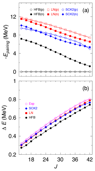
Figure 15: (a) Pairing energies (protons and neutrons) and (b) transition energies as a function of the cranking angular momentum, $J$, calculated with HFB, LN and SCK2 methods for ¹⁹⁰Hg with the Gogny D1S interaction. Experimental energies are also plotted in panel (b). Figure adapted from Refs. [108, 212].

Lipkin-Nogami method (instead of plain HFB) is still routinely used with Skyrme and RMF energy density functionals to find the intrinsic mean-field-like wave functions. This is mainly due to the problems that arise when the particle number symmetry restoration is implemented in EDFs that deal differently with the HF and pairing parts of functional [92, 213, 207, 202] (see Sec 5.1.4 for a discussion of this issue). A closer approach to PN-VAP energies can be obtained by projecting LN intrinsic mean-field states onto good number of particles exactly. This is the so-called projected Lipkin-Nogami approach (PLN). This method, compared to the full PN-VAP, is only able to approximate the minima of the PN projected energy surfaces defined along the direction of $\Delta N^{2}$ [214].

Nevertheless, Kamlah and Lipkin-Nogami methods with Gogny EDFs were quickly improved with the full implementation of the exact particle number projection both within the PN-PAV and PN-VAP approximations [92]. In Fig. 16 the energy difference between the ground-state energy provided by the PN-VAP method and HFB, PN-PAV, LN and PLN methods in the Sn isotopic chain is shown. We observe that the lowest ground-state energies are obtained with the PN-VAP method, i.e., the energy difference is always positive. Since PN-VAP, PN-PAV, HFB, and PLN are variational methods, the PN-VAP approach is the best one in that respect. In addition, the largest energy differences are obtained in the doubly-magic isotopes ^100,132Sn. In those nuclei, not only the proton but also the neutron pairing correlations collapse in the HFB approach and, subsequently, in the PN-PAV one. LN and PLN are able to attain some pairing correlations in the whole isotopic chain, but these shell effects are still present.

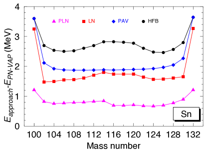
Figure 16: Difference between the ground state energies obtained with the PN-VAP method and HFB, LN, PN-PAV and PLN approaches in the Sn isotopic chain. Gogny D1S interaction is used. Figure adapted from Ref. [215].

Another way of studying the performance of these approaches with the Gogny force is represented in Fig. 17. Here, several potential energy surfaces of ⁵⁴Cr as a function of the quadrupole deformation are plotted (Fig. 17(a)), depending on the variational many-body method used to obtain the total energy of the nucleus. As previously, the best approach is given by the PN-VAP method and the PLN approach, although gives a similar qualitative result, is still above the PN-VAP result in the whole range of quadrupole deformations. Moreover, if we analyze the pairing energies, both for protons and neutrons, in connection with the corresponding single-particle-energies, we observe again that the largest amount of pairing correlations is obtained with the PN-VAP approach. The HFB and PN-PAV solutions show spurious super-fluid normal-fluid phase transitions for deformations for which the level density is small. This is not the case for the PLN method but this approximation is unable to capture enough pairing correlations in regions with small and large level density around the Fermi level.

Figure 17: (a) Energy (normalized to the minimum of the HFB solution) as a function of the axial quadrupole deformation in ⁵⁴Cr calculated with HFB, PN-PAV, PNL and PN-VAP approximations. (b)-(c) Single-particle-energies and (d)-(b) pairing energies as a function of the axial quadrupole deformation for protons (left panel) and neutrons (right panel), respectively. Gogny D1S interaction is used. Dash thick lines in (b) and (c) represent the Fermi level. Figure adapted from Ref. [216].

Despite the PN-VAP method is widely used in current EDF calculations, there is still one problem left when beyond-mean-field methods with density-dependent interactions are implemented, i.e., the definition of the spatial density that enters in the interaction. The density-dependent term in the Gogny interaction is $\propto\rho^{1/3}(\vec{R})$ (where $\vec{R}$ is the position of the center-of-mass of the two nucleon system) and in the HFB approximation the spatial density is defined unambiguously as $\rho(\vec{r})=\langle\Phi|\hat{\rho}(\vec{r})|\Phi\rangle$. However, it is not obvious how to extend the definition of this density in the case of particle number projection, or, more generally, in the generator coordinate method where matrix elements of operators between different HFB states on the left (bra) and right (ket) are used. Hence, two prescriptions have been used mainly in PNP implementations with Gogny interactions (see Sec 5.1.5 for a discussion), namely, the mixed density, $(\rho(\vec{r},\varphi))$, and the PN-projected density, $(\rho^{N}(\vec{r}))$:

$$\rho(\vec{r},\varphi) = \frac{\langle\Phi|\hat{\rho}(\vec{r})e^{i\varphi\hat{N}}|\Phi\rangle}{\langle\Phi|e^{i\varphi\hat{N}}|\Phi\rangle}$$ (102)

$$\rho^{N}(\vec{r}) = \frac{\langle\Phi|\hat{\rho}(\vec{r})\hat{P}^{N}|\Phi\rangle}{\langle\Phi|\hat{P}^{N}|\Phi\rangle}$$ (103)

In both cases rearrangement terms appear in the variational equations (exact and approximate as LN and/or SCK2) that have to be properly taken into account [108, 92]. Additionally, when the mixed prescription is used to compute the PNP energy obtained from the density-dependent term of the Gogny force (proportional to a non-integer power of the density), such a term is not well defined [213, 207, 202]. Nevertheless, the PN-projected density prescription has been used in practically all of the PNP calculations performed so far with the Gogny interaction. This prescription is free from these problems although it has a more phenomenological character than the mixed prescription.

Let us mention two other important implementations of exact particle-number restorations with Gogny EDFs. The first one is the study of the impact of the PNP on nuclear halos, skins and drip-lines including the continuum [217, 218]. These calculations were performed using a spherical Woods-Saxon basis and a restricted PN-VAP (R-PN-VAP) method as an approximation to the full PN-VAP one. Such a R-PN-VAP procedure consisted in: a) finding a set of HFB wave functions, $\{|\Phi(x)\rangle\}$, that minimize the HFB energy whose pairing field matrix, $\Delta(x)=x\Delta$, is multiplied by a pairing enhancement factor, $x$. Obviously, the HFB solution will be directly given by $x=1$; b) computing the PNP energy surface along the pairing enhancement factor, $\langle\Phi(x)|\hat{H}\hat{P}^{N}\hat{P}^{Z}|\Phi(x)\rangle$; and, c) selecting the minimum of the PNP energy surface as the total energy. It is shown in Refs. [217, 218] that the two-neutron drip line is extended by two neutrons in a half a dozen cases with respect to the drip line predicted with continuum HFB calculations. These cases correspond to closed-shell nuclei where, contrary to the HFB method, R-PN-VAP can still get pairing correlations and, therefore, a lower total energy that produces a positive two-neutron separation energy.

On the other hand, pairing fluctuations have been also included in the study of nuclear structure properties with Gogny EDFs [219, 220]. In this case, axial symmetric PN-VAP calculations have been performed along the quadrupole deformation and particle-number fluctuation ($\Delta N^{2}$) degrees of freedom on an equal footing. The inclusion of the latter degree of freedom allows, among other aspects, the study of pairing vibrations because states with the same spatial deformation but with different pairing gaps (”pairing deformations”) can be mixed. This mixing can generate states that ”vibrate” around an average pairing gap. Since these calculations serve as the starting point of more involved beyond-mean-field techniques (including not only particle number, but also angular momentum restoration, and configuration mixing) we will discuss this implementation in a subsequent Section (see Sec. 6.3).

5.4 Angular Momentum Projection (AMP)

Similarly to the particle-number symmetry breaking mechanism, the HFB wave functions can also break the rotational symmetry of the system by definition. This procedure enlarges the HFB variational space and allows the inclusion of correlations related to spatial multipole deformations of the Hamiltonian. However, the mean-field many-body wave functions (in general) are not eigenstates of the total nor the third component of the angular momentum operators, ($\hat{J}^{2},\hat{J}_{z}$), but a linear combination of them:

$$|\phi\rangle=\sum_{\alpha,JM}a_{\alpha,JM}|\alpha JM\rangle$$ (104)

where $|\alpha JM\rangle$ are eigenstates of ($\hat{J}^{2},\hat{J}_{z}$) and $\alpha$ refers to other quantum numbers of the system. This drawback can be corrected through symmetry restoration techniques (angular momentum projection, AMP) in a similar way as the particle-number symmetry discussed in Sec. 5.3. In this case, the projection methods are more involved since the symmetry group associated to rotations is more complex. Due to the large computational cost of the AMP, this kind of symmetry restoration has been only carried out in a PAV approach with the most sophisticated EDFs (Skyrme, Gogny, RMF). Thus, we can build an eigenstate of the angular momentum operators, ($\hat{J}^{2},\hat{J}_{z}$), applying a projection operator to a symmetry-breaking many-body state, $|\phi\rangle$ [84]:

$$|JM\sigma\rangle=\sum_{K=-J}^{J}g^{J\sigma}_{K}|JMK\rangle=\sum_{K=-J}^{J}g^{J\sigma}_{K}\hat{P}^{J}_{MK}|\phi\rangle$$ (105)

where $J$, $M$ and $K$ are the total angular momentum and the projection of $\vec{J}$ on the laboratory and intrinsic $z$-axes, respectively; $\hat{P}^{J}_{MK}$ is the angular momentum projector operator written in terms of an integral over the Euler angles ($\Omega=(\alpha,\beta,\gamma)$) [84].

$$\hat{P}^{J}_{MK}=\frac{2J+1}{16\pi^{2}}\int^{4\pi}_{0}d\alpha\int^{\pi}_{0}d\beta\sin\beta\int^{2\pi}_{0}d\gamma\mathcal{D}^{J*}_{MK}(\Omega)\hat{R}(\Omega)$$ (106)

with $\mathcal{D}^{J}_{MK}(\Omega)$ are the Wigner matrices and $\hat{R}(\Omega)=e^{-i\alpha\hat{J}_{z}}e^{-i\beta\hat{J}_{y}}e^{-i\gamma\hat{J}_{z}}$ is the rotation operator defined with the Euler angles. The interval of integration over the angle $\alpha$ can be reduced to $[0,2\pi]$ for even-even nuclei, multiplying Eq. 106 by a factor 2.

Furthermore, the coefficients $g^{J\sigma}_{K}$, with $\sigma=1,2,3,...$ labeling the different states for a given value of the angular momentum, are obtained by minimizing the angular momentum projected energy within the $K$-space of dimension $(2J+1)\times(2J+1)$ [84]. This is equivalent to solve a Hill-Wheeler-Griffin (HWG) equation (see Sec. 6.3) defined in such a space:

$$\sum_{K^{\prime}=-J}^{J}\left(\mathcal{H}^{J}_{KK^{\prime}}-E^{J\sigma}\mathcal{N}^{J}_{KK^{\prime}}\right)g^{J\sigma}_{K^{\prime}}=0$$ (107)

The projected norm and Hamiltonian overlaps are defined as:

$$\mathcal{N}^{J}_{KK^{\prime}} = \langle\phi|\hat{P}^{J}_{KM}\hat{P}^{J}_{MK^{\prime}}|\phi\rangle=\langle\phi|\hat{P}^{J}_{KK^{\prime}}|\phi\rangle$$

$$\mathcal{H}^{J}_{KK^{\prime}} = \langle\phi|\hat{P}^{J}_{KM}\hat{H}\hat{P}^{J}_{MK^{\prime}}|\phi\rangle=\langle\phi|\hat{H}\hat{P}^{J}_{KK^{\prime}}|\phi\rangle$$ (108)

These equations are trivially obtained from the commutation properties, $[\hat{\mathcal{I}},\hat{R}(\Omega)]=0,[\hat{H},\hat{R}(\Omega)]=0$, and the property of the angular momentum projector $\hat{P}^{J}_{KM}\hat{P}^{J}_{MK^{\prime}}=\hat{P}^{J}_{KK^{\prime}}$. However, the last expression in Eq. 108 must be taken with care when we deal with density-dependent interactions since the density-dependent term is not, in general, rotational invariant. As discussed thoroughly in Ref. [221], the mixed-density prescription fulfills two basic requirements to provide a meaningful AMP energy, i.e., this term should produce: a) a scalar quantity (it should not carry angular momentum); and, b) a real (non-complex) quantity. The mixed-density prescription is defined in the AMP case as:

$$\rho_{\Omega}(\vec{r})=\frac{\langle\phi|\hat{\rho}(\vec{r})\hat{R}(\Omega)|\phi\rangle}{\langle\phi|\hat{R}(\Omega)|\phi\rangle}$$ (109)

Again, as discussed in Secs. 5.1.5 and 5.3, this term could be ill-defined whenever a non-integer power of the density is used to evaluate the energy (e.g., 1/3 as in Gogny EDFs) [204, 213, 207, 202]. However, the suitability of this prescription has been only tested numerically (see Ref. [220]) and a more detailed work along the lines of Refs. [207, 204] but in the AMP context should be performed in the future. From now on, all the results that refer to angular momentum projected energies will be obtained by using the mixed-density prescription given by Eq. 109.

The calculation of the overlaps (Eq. 108) requires a three dimensional integration over the Euler angles:

$$\mathcal{N}^{J}_{KK^{\prime}} = \frac{2J+1}{16\pi^{2}}\int\mathcal{D}^{J*}_{KK^{\prime}}(\Omega)\langle\phi|\hat{R}(\Omega)|\phi\rangle d\Omega$$

$$\mathcal{H}^{J}_{KK^{\prime}} = \frac{2J+1}{16\pi^{2}}\int\mathcal{D}^{J*}_{KK^{\prime}}(\Omega)\langle\phi|\hat{H}\hat{R}(\Omega)|\phi\rangle d\Omega$$ (110)

with $d^{J}_{KM}(\beta)$ the reduced Wigner matrices. Such a calculation can be largely simplified if the intrinsic many-body states, $|\phi\rangle$, are axially-symmetric, i.e., $\hat{J}_{z}|\phi\rangle=K|\phi\rangle$. For the even-even case, we can choose the $z$-axis along the symmetry axis, having $K=0$. Therefore, Eq. 110 is reduced to the evaluation of only one integral:

$$\mathcal{N}^{J}_{00} = \frac{2J+1}{2}\int_{0}^{\pi}d^{J*}_{00}(\beta)\langle\phi|e^{-i\beta\hat{J}_{y}}|\phi\rangle\sin\beta d\beta$$

$$\mathcal{H}^{J}_{00} = \frac{2J+1}{2}\int_{0}^{\pi}d^{J*}_{00}(\beta)\langle\phi|\hat{H}e^{-i\beta\hat{J}_{y}}|\phi\rangle\sin\beta d\beta$$ (111)

Furthermore, the HWG equation (Eq. 107) is trivially solved because it just expresses the single value obtained for the AMP energy in the axial case.

Most of the implementations of the AMP with Gogny interactions has been considered as an intermediate step from constrained HFB or PN-VAP towards configuration mixing (within the generator coordinate method) calculations. Nevertheless, we present some relevant properties of the AMP itself and the main differences/similarities between the calculations that have been published so far.

First developments of the AMP with Gogny interactions were applied to the study of super-deformed bands and collectivity around $N=20$ and $N=28$ magic numbers in light nuclei, as well as the description of shape coexistence in the neutron-deficient lead region [222, 221, 223, 224]. These calculations assumed HFB many-body states with axial, parity and time-reversal symmetry conservation. These intrinsic HFB states were obtained from constrained-HFB calculations along the axial quadrupole degree of freedom ($q_{20}$), although some other directions -respecting axial, parity and time-reversal symmetries- were also explored [225]. Particle number projection was not performed in these calculations either. Therefore, the AMP energy surfaces were evaluated as:

$$E^{J}(q_{20})=\frac{\mathcal{H}^{J}_{00}(q_{20})}{\mathcal{N}^{J}_{00}(q_{20})}-\sum_{\tau=p,n}\lambda_{N_{\tau}}(q_{20})\left(\frac{(\mathcal{N}_{\tau})^{J}_{00}(q_{20})}{\mathcal{N}^{J}_{00}(q_{20})}-N_{\tau}\right)$$ (112)

where $\frac{(\mathcal{N}_{\tau})^{J}_{00}(q_{20})}{\mathcal{N}^{J}_{00}(q_{20})}$ is the AMP expectation value of the number of protons ($\tau=p$) and neutrons ($\tau=n$), $\lambda_{N_{\tau=p,n}}$ are the Lagrange multipliers obtained in the constrained-HFB calculation and $N_{\tau=p,n}$ are the actual number of protons and neutrons of the nucleus under study.

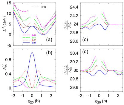
Figure 18: (a) Energy (normalized to the minimum of the $J=0$ solution) as a function of the axial quadrupole deformation in ⁵⁴Cr calculated with HFB and HFB+AMP with $J=0^{+}$, $2^{+}$, $4^{+}$ and $6^{+}$ methods with Gogny D1S. (b) AMP norm overlap and expectation values of the number of (c) protons and (d) neutrons as a function of the axial quadrupole deformation for $J=0^{+}$, $2^{+}$, $4^{+}$ and $6^{+}$.

We show the main aspects of a HFB+AMP calculation in Fig. 18 along the axial quadrupole moment, where the nucleus ⁵⁴Cr is used as an example. In Fig. 18(a) the potential energy surfaces (PES) are represented for the results obtained with the constrained-HFB method and the subsequent AMP with $J=0^{+}$, $2^{+}$, $4^{+}$ and $6^{+}$. For $J=0^{+}$ we observe an energy gain with respect to the HFB solution, except for the spherical point ($q_{20}=0$). Therefore, we obtain a correlation energy due to the rotational symmetry restoration of deformed nuclei. In addition, the two minima (one prolate and one oblate) found in the HFB calculation are also obtained in the AMP-PES but shifted to larger deformations. Thus, the PES without AMP are always modified by the inclusion of the angular momentum projection. This modification can significantly change the character of the nucleus under study in those cases where two minima, one less deformed (or spherical) than the other, are obtained in PES without AMP. A paradigmatic example of this effect is the nucleus ³²Mg. Since this nucleus has $N=20$ neutrons (magic number), the HFB-PES has its absolute minimum in the spherical point and a shoulder related to the crossing of neutron $f_{7/2}$ and $d_{3/2}$ orbits appears at $q_{20}\approx 0.8$ b (see Fig. 19 and Ref. [124]). However, once the angular momentum projection is performed, the absolute minimum corresponds now to a prolate deformed state, in agreement with the structure inferred from experiments.

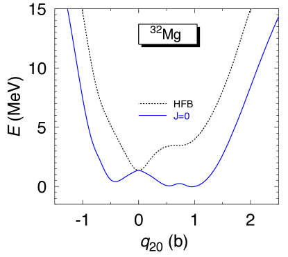
Figure 19: (a) Energy (normalized to the minimum of the $J=0$ solution) as a function of the axial quadrupole deformation in ³²Mg calculated with HFB and HFB+AMP with $J=0^{+}$ methods. Gogny D1S is used. Adapted from Ref. [124].

Coming back to the ⁵⁴Cr example, we observe in Fig. 18(a) that the AMP-PES with $J\neq 0^{+}$ present discontinuities around $q_{20}=0$. Their origin is the same as the zero energy gain in the spherical point for $J=0^{+}$ and the absence of negative parity and odd-$J$ states. The projected norm overlap shown in Fig. 18(b) represents the probability of finding a given eigenstate of the angular momentum in a intrinsic state. Using the decomposition given in Eq. 104, we see that such a probability is:

$$P(JM)=\sum_{\alpha}|\langle\alpha JM|\phi\rangle|^{2}=\sum_{\alpha}|a_{\alpha,JM}|^{2}=\mathcal{N}^{J}_{00}$$ (113)

Since the underlying HFB states are axial and parity symmetric, only positive parity and even-$J$ angular momentum projected states can be obtained. In other words, the coefficients of the linear combination given in Eq. 104 for negative parity and odd-$J$, i.e., their projected norm overlaps, are strictly zero in this case. In addition, the spherical intrinsic state, $|\phi(q_{20}=0)\rangle$, is already an eigenstate of the angular momentum operators with $J=0$. Therefore, the projected norm overlap for $J=0$ is one, and zero for other values of $J$ (see Fig. 18(b)). This is the reason why there is not an energy gain in this special point by projecting onto $J=0$ and the appearance of the gap in the $J\neq 0$ PES around this deformation.

Finally, on the right panel of Fig. 18 we plot the projected expectation values of the number of protons and neutrons. Here we observe a non-negligible deviation from the nominal values for ⁵⁴Cr. In fact, the deformations for which the number of protons/neutrons is correct correspond to regions where the HFB method presents a phase transition to HF solutions (without pairing). From this plot it is already obvious that if we want to perform more reliable beyond-mean-field calculations, the PNP must be also carried out.

This simultaneous particle number and angular momentum projection (PNAMP) was first implemented with Gogny EDFs in Ref. [216] as part of a more general beyond-mean-field method to study the potential $N=32$ and $N=34$ shell closures in neutron rich calcium, titanium and chromium isotopes. One of the main advantages introduced here was that the PNAMP was performed onto intrinsic HFB-like wave functions that are obtained from constrained PN-VAP instead of plain constrained-HFB calculations. This fact improved the pairing properties of the method. Therefore, the intrinsic many-body states in Eq. 105 have the form of Eq. 96. As in the previous case, in the first applications of the PNAMP with Gogny interactions, axial, parity and time-reversal symmetries were conserved to reduce the computational burden. Nevertheless, these restrictions have been overcome in the most recent developments as we discuss below.

A major improvement of PNAMP calculations with Gogny EDFs was the implementation of the triaxial angular momentum projection for even-even nuclei in Ref. [226]. Again, parity and time-reversal symmetries were not broken, or, more specifically, $D^{T}_{2h}$ symmetry was conserved [227, 228, 229]. Therefore, the $(\beta_{2},\gamma)$ plane can be reduced to values of $\gamma\in[0^{\circ},60^{\circ}]$. Many details such as the convergence of the triaxial AMP with respect to the number of Euler angles used to discretize the three-dimensional integral (Eq. 106) or the best choice of the mesh in the $(\beta_{2},\gamma)$ plane are discussed thoroughly in Ref. [226]. The inclusion of triaxiality opened several possibilities, for example: the study of shape evolution, mixing and/or coexistence in a more appropriate way; the study of $\gamma$-bands and $J^{+}$-odd states; a better description of $J\neq 0$ excited states through $K$-mixing, etc.. These applications will be reviewed in Sec. 6.3.

Let us show in three examples how the inclusion of the triaxial degree of freedom could change the interpretation of the potential energy surfaces obtained with an axial calculation. In Fig. 20(a)-(c) PN-VAP and PNAMP ($J=0$) results for the nucleus ²⁴Mg are plotted. We observe that, in the axial case (Fig. 20(a)), both the PN-VAP and $J=0$ PES have two well-defined minima, one prolate (the absolute one) and one oblate. These minima are shifted to slightly larger values in the AMP case. If we now explore additionally the triaxial degree of freedom we see that there is only one minimum, i.e., the prolate one in the PN-VAP case (Fig. 20(b)) that is displaced towards larger and more triaxial deformations when AMP is performed (Fig. 20(c)). Therefore, the axial oblate minimum is actually a saddle point in the $(\beta_{2},\gamma)$ plane. The situation is even worse in nuclei where a well-defined triaxial minimum is found in the triaxial-PES as in the isotope ¹²⁶Xe Fig. 20(d)-(f). Two minima (oblate and prolate) very close in energy are obtained in the axial PN-VAP and $J=0$ PES. This result could be interpreted as a possible signature of shape coexistence and/or shape mixing. However, if we study the triaxial PES, we see that these minima correspond to the saddle points produced by the absolute (and single) triaxial minimum. Finally, in Fig. 20(g)-(i) we show an example (⁷⁴Kr) of a more plausible case of shape coexistence. Here, actual axial oblate and prolate minima are obtained in the PN-VAP axial and triaxial calculations. However, the $J=0$ surfaces show again differences between the axial and triaxial results exploring the triaxial degree of freedom. Hence, the barrier between prolate and oblate configurations is much smaller through pure triaxial configurations and the absolute minimum is located at a more prolate deformation in the triaxial case than in the axial calculation, that corresponds to an oblate shape.

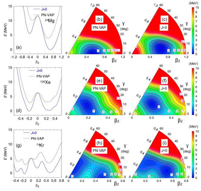
Figure 20: Left panel: PN-VAP and PNAMP ($J=0$) potential energy surfaces (normalized to the absolute minimum of the $J=0$ PES) calculated with axially symmetric intrinsic wave functions. Middle panel and right panels: PN-VAP and PNAMP ($J=0$) potential energy surfaces (normalized to their minima) in the triaxial $(\beta_{2},\gamma)$ plane, respectively. Calculations are performed with Gogny D1S EDF for (a)-(c) ²⁴Mg, (d)-(f) ¹²⁶Xe and (g)-(i) ⁷⁴Kr isotopes.

Apart from the inclusion of triaxial shapes, the octupole degree of freedom has been recently explored in PNAMP calculations with Gogny EDFs [230, 231]. These states break the parity symmetry. Therefore, a simultaneous parity, particle number and angular momentum projection (PPNAMP) is also carried out. The intrinsic many-body states in Eq. 105 are thus parity and particle number projected HFB-like wave functions, $|\phi\rangle=\hat{P}^{N}\hat{P}^{Z}\hat{P}^{\pi}|\psi\rangle$ ($\hat{P}^{\pi}$ is the parity projection operator [84]). This method is used to study regions of the nuclear chart where the octupole correlations are expected to play an important role. In addition, both positive and negative parity states can be computed within this approach.

The possible appearance of tetrahedral shapes in the region of Zr isotopes has been examined analyzing PPNAMP potential energy surfaces along axial and non-axial deformations [230]. In this case, a full triaxial angular momentum projection is also included. On the other hand, PPNAMP potential energy surfaces have been studied in the Ba region as the intermediate step of configuration mixing calculations [231]. Here, only axial-symmetric HFB wave functions have been considered. We show in Fig. 21 an example of the performance of the PPNAMP method in the nucleus ¹⁴⁴Ba. First of all, the PES along the $(\beta_{2},\beta_{3})$ plane are symmetric by exchanging $\beta_{3}\rightarrow-\beta_{3}$ due to the parity conservation of the nuclear interaction. This isotope is found to be both quadrupole and octupole deformed already within the mean-field approximation. The main effects of the simultaneous PPNAM projection are: a) the widening of the potential wells around the absolute minima; b) the connection between prolate and oblate configurations through the octupole degree of freedom direction for $J=0^{+}$; and, c) an energy gain of $\sim 4.5$ MeV of correlation energy (difference between the HFB and $J=0^{+}$ absolute minima). Additionally, projection to odd-angular momenta and negative parity is not possible for the intrinsic states with $\beta_{3}=0$ since the projected norm overlaps for those parity- and axially-symmetric wave functions are zero.

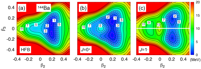
Figure 21: Potential energy surfaces in the $(\beta_{2},\beta_{3})$ plane for (a) HFB, (b) PPNAMP-$J=0^{+}$ and (c) PPNAMP-$J=1^{-}$ approximations computed for ¹⁴⁴Ba with the Gogny D1S parametrization. PES are normalized to the energy of the minimum of (a) HFB and (b)-(c) PPNAMP-$J=0^{+}$ surfaces. Contour lines are separated by 0.5 MeV (dashed lines) and 2.0 MeV (continuous lines) respectively. Adapted from Ref. [231].

The last implementation of simultaneous particle number and angular momentum projections with Gogny EDFs has been carried out onto intrinsic wave functions that break the time-reversal symmetry. These developments have been applied to study both even-even nuclei -with intrinsically rotating wave functions (cranking) [232, 32, 233, 234, 235, 3]- and odd-even nuclei -with blocking [236, 237]. As a consequence of the time-reversal symmetry breaking, the equivalence of the six sextants in the $(\beta_{2},\gamma)$ plane is lost ($D^{T}_{2h}$ symmetry is broken [227, 228, 229]). In cranking calculations, where the intrinsic wave functions are constrained to have, for example, $\langle\hat{J}_{x}\rangle=\sqrt{J_{c}(J_{c}+1)}$, it is usual to keep the simplex as a self-consistent symmetry ($\hat{\Pi}e^{-i\pi\hat{J}_{x}}|\rangle=|\rangle$, with $\hat{\Pi}$ the parity operator). Therefore, the $(\beta_{2},\gamma)$ plane is divided now in two equivalent sextants that are symmetric with respect to the $\gamma=(120^{\circ},300^{\circ})$ direction (because the cranking direction is chosen to be the $x$-axis). This property can be used to perform consistency checks of the PNAMP with cranking wave functions as it is shown in Ref. [232]. In Fig. 22(a)-(b) we show energy surfaces in the whole $(\beta_{2},\gamma)$ computed for the ³²Mg isotope with the PN-VAP method with cranking. Two different values of the cranking angular momentum, $J_{c}=0$ and 4, are chosen to discuss the effect of time-reversal symmetry breaking in this kind of calculations. Furthermore, these intrinsic states are also angular momentum projected and the corresponding PES for $(J_{c}=0,J=0)$ and $(J_{c}=4,J=4)$ are plotted in Fig. 22(c)-(d). We observe (left panel) that, as anticipated, the six sextants of PES computed with $J_{c}=0$ are equivalent. This is not the case for the PES calculated with $J_{c}=4$ (right panel). Since the cranking method produces intrinsically rotating deformed states about the $x$-axis, thus, the energies are not independent on the orientation of the coordinate system. Therefore, a better description of the nucleus is obtained by exploring three sextants of the $(\beta_{2},\gamma)$ plane. This has been already implemented with Gogny EDFs to study isomeric states in ⁴⁴S [32] and ⁴²Si [3] since, due to the intrinsic rotations, single-particle excitations associated to alignments can be obtained within the PNAMP plus cranking approach.

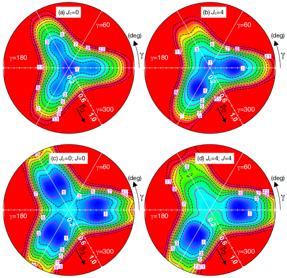
Figure 22: (a) Energy as a function of the quadrupole $(\beta_{2},\gamma)$ deformation in ³²Mg calculated with (a)-(b) PN-VAP and (c)-(d) PNAMP methods. In (a) and (c) the cranking angular momentum is $J_{c}=0$ while in (b) and (d) it is $J_{c}=4$. Gogny D1S is used. Adapted from Ref. [232].

As mentioned above, PNAMP energy surfaces have been also calculated with blocking (one-quasiparticle) PN-VAP states [236, 237]. These works constitute the first implementations of PNAMP for odd-nuclei with Gogny EDF. In particular, bulk properties and electromagnetic moments were computed for the magnesium isotopic chain, obtaining a good agreement with the experimental data. Figure 23 shows the PNAMP-PES corresponding to the angular momentum that provides the ground state energy for each isotope. Obviously, this value corresponds to $J=0^{+}$ for even systems while for odd systems, several blocking configurations (only neutrons of both positive and negative parity) were explored to find the predicted ground state.

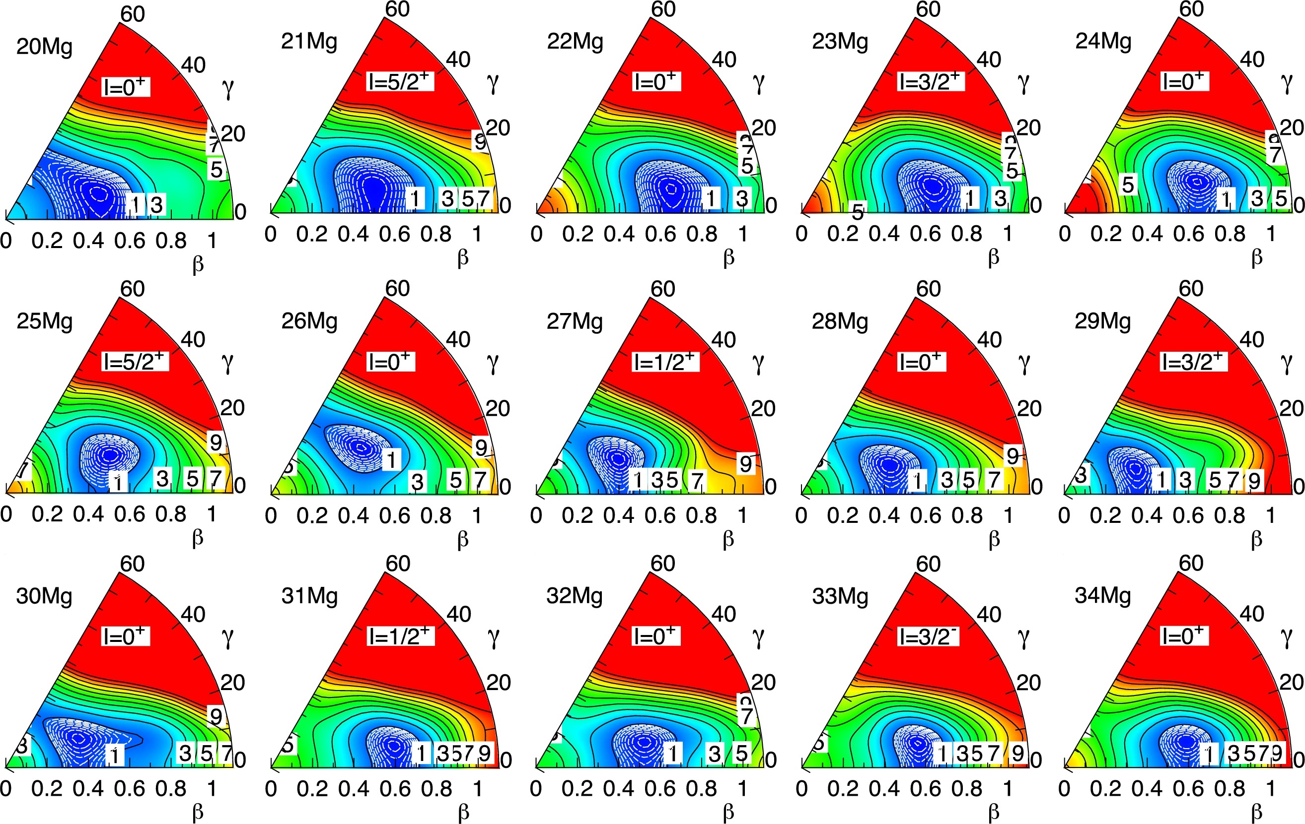
Figure 23: Particle number and angular momentum projected potential energy surfaces (normalized to each minimum) as a function of $(\beta_{2},\gamma)$ Mg isotopic chain including both even-even and odd-even nuclei with the Gogny D1S interaction. The angular momentum is chosen to be the one that gives the ground state for each isotope. Figure taken from Ref. [237].

Let us finish this section with two important comments. The first one is that the variation after angular momentum projection (AM-VAP) is far from being reached with sophisticated EDFs as Gogny. However, the exploration of AM-PAV energy surfaces defined along different degrees of freedom (quadrupole, octupole, cranking rotation, etc.) can be considered as a meaningful approach to the full VAP. In fact, a restricted VAP (RVAP) can be performed by choosing the minima of the AM-PAV energy surfaces. The second comment concerns the prescription for the spatial density in PNAMP calculations with Gogny EDFs. This was phenomenologically taken as a mixed version of projected (in the particle number projection) and mixed (in the angular momentum projection) prescriptions:

$$\rho^{NZ}_{\Omega}(\vec{r})=\frac{\langle\phi|\hat{\rho}(\vec{r})\hat{R}(\Omega)\hat{P}^{N}\hat{P}^{Z}|\phi\rangle}{\langle\phi|\hat{R}(\Omega)\hat{P}^{N}\hat{P}^{Z}|\phi\rangle}$$ (114)

This prescription has been used in all of the applications of PNAMP approaches presented above and also in the symmetry conserving configuration mixing (SCCM) approaches that will be presented in Sec. 6.3.

5.5 Linear momentum projection (Brink-Boecker force)

Although the Gogny force is not invariant under Galilei transformations owing to the phenomenological density dependent term, the consequences of the restoration of Galilei invariance on physical observables are important and therefore we have discussed them with a simplified nuclear interaction that shares its central potential with the Gogny force, the Brink-Boecker interaction [9].

The restoration of Galilei invariance is considered one of the most challenging symmetry restorations within the nuclear many-body problem. The homogeneity of space requires that the total linear momentum of the nucleus, considered as a closed system of interacting, non-relativistic nucleons, is conserved. Therefore, the Hamiltonian cannot depend on the center of mass (COM) coordinate of its constituents, but only on relative coordinates and momenta. The dependence on the total linear momentum just accounts for the free motion of the system as a whole and can always be transformed away by considering the COM rest frame. In principle, the remaining (internal) Schrödinger equation can be solved by writing the Hamiltonian in Jacobi coordinates. However, since nucleons obey the Pauli principle and the Jacobi coordinates depend on all the nucleon coordinates, an explicit anti-symmetrization of the wave function should be carried out. Such an explicit anti-symmetrization, thought still feasible in few-body systems, becomes impossible for systems with a large number of nucleons. In this case, anti-symmetrization is then taken into account implicitly by considering (mean-field) product trial wave functions [84] that automatically incorporate Pauli’s principle. Nevertheless, those product wave functions depend on 3A instead of the allowed 3A-3 coordinates and thus contain spurious contaminations due to the motion of the system as a whole. As a result, Galilei invariance is broken. This fact was already recognized [238] as one of the problems of the nuclear shell model. It also was shown [239] that for pure harmonic oscillator configurations the problem can be treated by diagonalizing the (oscillator) COM Hamiltonian and projecting out of the spectrum all states not corresponding to the ground state of this operator. However, this requires the use of complete $n\hbar\omega$ spaces since only then COM and internal excitations decouple exactly.

A more general solution is obtained via symmetry restoration [196, 240, 200, 84], i.e., by projecting the considered wave functions into the COM rest frame. Note, that the projection techniques only ensure translational invariance and in order to recover the full Galilei invariance, the projection into the COM rest frame should be carried out before solving the corresponding mean-field (variational) equations [84], i.e., full Galilei invariance can only be recovered if the projection into the COM rest frame is carried out before the variation.

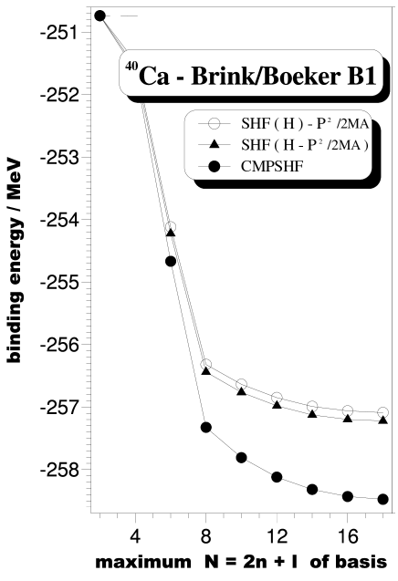
Figure 24: Total binding energy of ⁴⁰Ca plotted as a function of the size of the single particle basis. Three curves are shown in the plot: the open circles correspond to a normal spherical Hartree-Fock calculation with the expectation value of ${\hat{P}}/2MA$ subtracted after convergence is achieved, the full triangles correspond to a calculation in which this COM correction is included in the variational procedure and the full circles correspond to a spherical Hartree-Fock calculation with projection into the COM rest frame before the variation. Taken from Ref. [241].

The COM projection method works in general model spaces as well as for general wave functions. However, it also entails challenging technical difficulties. For example, the associated projection operator links states in the model space to those in the core because any change of the momentum of the valence nucleons should be accompanied by a change in the momentum of the core to ensure zero total linear momentum. In other words, unlike other nuclear symmetries, linear momentum is a true A-body correlation and hence more difficult to afford than other symmetry restorations.

The previous difficulties might be the main reasons why the exact restoration of Galilei invariance in the nuclear many-body problem has received much less attention in comparison with other symmetries. Instead, approximations like subtracting the kinetic energy of the COM from the original Hamiltonian which is in the definition of the Gogny force or the Tassie-Barker [242] corrections to form factors are commonly employed. However, previous Hartree-Fock calculations with projection onto the COM rest frame in the case of ⁴He [243] as well as for form factors and charge densities in spherical nuclei [244, 245] have shown, that a correct treatment of Galilei invariance leads to effects far beyond the usually assumed 1/A dependence. Considerable effects have also been found for scattering states in ⁴He [246] as well as for spectral functions, spectroscopic factors, transition form factors and densities, energies of hole states, Coulomb sum rules and response functions in Refs. [247, 248, 249, 250].

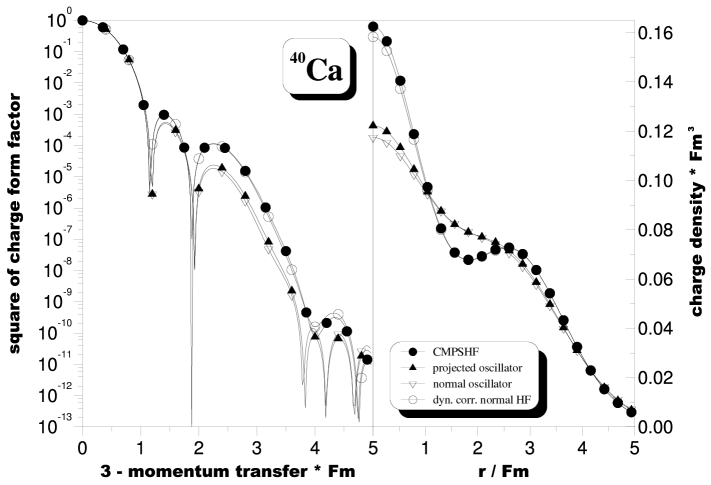
Figure 25: In the left panel of the figure the square of the charge form factor for ⁴⁰Ca is displayed as a function of the 3-momentum transfer. Open inverted triangles correspond to an oscillator occupation with no COM correction included, full triangles give the oscillator result including the Tassie-Barker factor (projected oscillator), open circles display the form factor obtained with the normal Hartree-Fock (including COM correction in the Hamiltonian during the variation) taking into account the dynamic correction Eq.(122) in the main text. Full circles display the result of the full VAP-projected calculation. The right part of the figure shows the corresponding charge densities. Taken from Ref. [241].

In order to obtain a Galilei invariant wave function, the following ansatz is used

$$|\Phi\,;\;0\rangle\,\equiv\,{{\hat{C}(0)|\Phi\rangle}\over{\sqrt{\langle\Phi|\hat{C}(0)|\Phi\rangle}}}$$ (115)

as a trial variational state. The operator

$$\hat{C}(0)\,\equiv\,\int d^{3}\,\vec{a}\,\exp\{i\vec{a}\cdot\hat{P}\}$$ (116)

projects into the COM rest frame by superposing all shifted (by $\vec{a}$) states $\exp\{i\vec{a}\cdot\hat{P}\}|\Phi\rangle$ with identical weights. The operator $\hat{P}$ in the exponent is the operator of the total linear momentum. The state $|\Phi\rangle$ represents a Slater determinant that is determined as the one minimizing [251] the projected energy

$$E_{\mathrm{proj}}\;={{\langle\Phi|\hat{H}\hat{C}(0)|\Phi\rangle}\over{\langle\Phi|\hat{C}(0)|\Phi\rangle}}$$ (117)

As an example of the performance of the COM projection, we analyze the results of spherical HF calculations with a Gogny-like interaction without the density-dependent term. The effect of the symmetry restoration on the total energy of the nucleus ⁴⁰Ca is shown in Fig. 24. Here, the total energy as a function of the size of the single particle basis is represented for three different calculations , namely: a) HF calculations with the subtraction of the expectation value of the kinetic energy of the COM motion afterwards; b) HF calculations where the minimization of the energy is carried out with a modified Hamiltonian given by $\hat{H^{\prime}}=\hat{H}-\frac{\hat{P}^{2}}{2MA}$; and, c) projection onto the COM rest frame before the variation. As can be seen from the figure, in the case of pure oscillator occupations (i.e., the smaller basis) the three curves coincide, as expected, since these are non spurious configurations. With increasing basis size, however, they display a rather different major shell mixing. The two curves for the unprojected approaches, i.e., solutions a) and b), run almost parallel with the latter providing a larger binding energy than the former. Furthermore, the energy gain of the projected approach is the largest among all of the methods and, as we observe in the figure, this contribution to the total energy is not negligible even in a not-so-light system as ⁴⁰Ca.

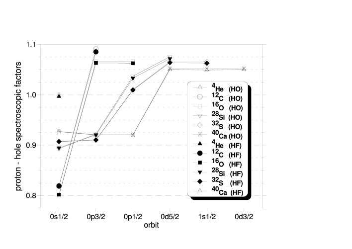
Figure 26: Proton-hole-spectroscopic factors for the various spherical hole-orbits in ⁴He, ¹²C, ¹⁶O, ²⁸Si, ³² and ⁴⁰Ca. Open symbols refer to the projected results using pure harmonic oscillator occupations. For ³²S and ⁴⁰Ca the $0s_{1/2}$ denotes orthonormalized states (with respect to the $1s_{1/2}$ orbit). Full symbols refer to results obtained with projection into the COM rest frame before the variation. In this case $0s_{1/2}$ denotes the lowest $s_{1/2}$ solution, $1s_{1/2}$ the second lowest $s_{1/2}$ solution and for the other orbits $0lj$ always the lowest solution is meant. Note, that in the usual approximation all the numbers displayed in the figure should be 1 regardless of whether pure oscillator or projected Slater determinants are used. Taken from Ref. [252]

Other interesting observables that are sensitive to Galilei invariance restoration are the charge form factors and the charge densities. The charge density in momentum space [248, 253] is given by

$$\hat{\rho}_{n}\,\equiv\,\sum_{\tau=p,n}f_{\tau}(Q^{2})\,\sum_{i=1}^{N_{\tau}}\,\exp\{i\vec{q}\cdot\vec{r}_{i}\}$$ (118)

where $f_{\tau}(Q^{2})$ are the nucleon charge form factors as functions of the (negative) square of the four-momentum transfer $Q^{2}$ [241]. In the case of a Slater determinant $|\Phi\rangle$, the charge form factor in this approximation reads

$$F_{ch}^{n}(Q^{2})\,=\,\langle\Phi|\hat{\rho}_{n}|\Phi\rangle$$ (119)

and the corresponding charge density can be obtained via the Fourier transform of Eq.(119). On the other hand, the translationally invariant charge density reads [248, 241]

$$\hat{\rho}_{inv}\,\equiv\,\hat{\rho}_{n}\,\exp\{-i\vec{q}\cdot\vec{R}\}.$$ (120)

and, using Eq.(120), the Galilei-invariant charge form factor takes the form

$$F_{ch}^{pr}(Q^{2})\,=\,{{\langle\Phi|\hat{\rho}_{inv}\hat{C}(0)|\Phi\rangle}\over{\langle\Phi|\hat{C}(0)|\Phi\rangle}}$$ (121)

Obviously, the charge density corresponding to this form factor can be obtained through its Fourier transform. On the other hand, if the Gaussian overlap approximation (GOA) [84] is applied to both the shift operator and the operator of Eq.(120), one obtains the dynamically corrected charge form factor

$$F_{ch}^{dy}(Q^{2})\,=\,F_{ch}^{n}(Q^{2})\,\exp\left\{{3\over 8}\,{{{\vec{q}\,}^{2}}\over{\langle\Phi|{\hat{P}\,}^{2}|\Phi\rangle}}\right\}$$ (122)

Note that when the Slater determinant corresponds to a non spurious state, then the exponent in Eq.(122) takes the form $\exp\{(\vec{q}\,b/2)^{2}/A\}$ which is the Tassie-Barker correction [242, 241].

These quantities are represented in Fig. 25 again for ⁴⁰Ca. In particular, Eq. 119 and Eq. 121 are evaluated with the spherical HF solution denoted by a) above (inverted open and full triangles respectively). The latter result is nothing but a PAV approach. Additionally, Eq. 122 is evaluated with the HF solution with the corrected Hamiltonian, referred as b) above. Finally, Eq. 121 has been computed with the VAP (Eq. 117) approximation. Charge form factors and their corresponding charge densities (Fourier transformations) are given on the left and right side of Fig. 25 respectively. Here we observe clearly the difference between pure mean-field and PAV approaches with the full COM-VAP restoration. Interestingly, the dynamically corrected form factor provides a very good approximation to the projection before the variation results, at least in the present nucleus.

Finally, let us consider the spectroscopic factors. They play a key role in one-nucleon transfer reactions where they are used to study nucleon-nucleon correlations. The normal hole-spectral functions $f_{h\tau\sigma}^{nor}(\vec{k}\,)$ are essentially given by the complex conjugate of the Fourier transform of the corresponding single particle wave functions [252]. The normal hole-spectroscopic factor is defined as

$$S_{h}^{nor}\,\equiv\,\sum\limits_{\sigma}\int d^{3}\vec{k}\,|f_{h\tau\sigma}^{nor}(\vec{k}\,)|^{2}$$ (123)

and satisfies the sum rule

$$\sum\limits_{h}S_{h}^{nor}\,=\,A$$ (124)

In the usual picture, the hole-spectroscopic factors are one for all the occupied states and zero for the unoccupied ones. However, such a picture is not Galilei-invariant and therefore requires a reformulation [252] where Galilei-invariant hole states $\overline{h}$ have to be considered in the projected hole-spectral functions $f_{\tilde{h}\tau\sigma}^{proj}(\vec{k}\,)$ and forms factors $S_{\tilde{h}}^{proj}$ The projected hole-spectroscopic factors satisfy a new sum rule

$$\sum\limits_{\tilde{h}}\,S^{proj}_{\tilde{h}}\,=\,A\,-\,\epsilon$$ (125)

where the ratio $\epsilon/A$ varies between 0.12 and 0.35 percent for the cases discussed in Ref. [252]. Therefore, the violation of the sum rule Eq.(124) due to the correlations induced by the projection operator on the uncorrelated Hartree-Fock system, is rather small.

The hole-spectroscopic factors for several $N=Z$ nuclei are depicted in Fig. 26. In the non-projected HF approximation they are all equal to one. Therefore, in the figure only projected hole-spectroscopic factors, both for the oscillator occupations [247] and the Hartree-Fock ground states are shown. Moreover, the proton and neutron spectroscopic factors are identical in the oscillator approach and even quite similar in the Hartree-Fock approach. Therefore, only results for protons are shown in the figure. As can be seen from the figure the oscillator and Hartree-Fock results are quite similar suggesting that the size of the single particle basis is not relevant in the Galilei-invariant prescription at least as long as only uncorrelated system are considered.

A considerable depletion of the strengths of the hole-states with excitation energies larger or equal to $1\hbar\omega$ and an enhancement of the strengths of the hole-orbits near the Fermi energy is observed. The oscillator results fulfill the sum rule Eq.(124) exactly, while for the HF determinants this is only approximately true Eq.(125). However, the violation $\epsilon$ of the sum rule is rather small.

The results presented in Fig. 26 suggest that the usual picture of an uncorrelated system has to be modified considerably. In particular, those results indicate that the interpretation of experiments in which deviations of the hole-spectroscopic factors from one are usually regarded as fingerprints of nucleon–nucleon correlations, should be taken with care. In a Galilei-invariant description, the spectroscopic factors even of an uncorrelated system differ from one and only deviations from the COM-projected results should be related to non-trivial nucleon-nucleon correlations.

The results discussed in this section illustrate that a correct treatment of Galilei invariance is possible, via projection techniques, in the case of finite range forces and large configuration spaces. They also suggest that, in the long run, the up to now almost neglected restoration of Galilei invariance should be incorporated in more sophisticated approaches like the shell model [254], the quantum Monte Carlo diagonalization method [255] and in symmetry-projected (mean-field based) methods [256]. For a more detailed account of these aspects, the reader is referred to Refs. [241, 252, 247, 248, 249, 250]. To the best of our knowledge, those COM-projected results still represent the only ones of their kind available in the literature.

5.6 Approximate versus exact projection

Symmetry restoration requires the evaluation of multidimensional integrals where the integrand is an overlap of operators that is expensive to compute (see Ref [235] for a discussion on computational costs). As this has to be repeated for many overlaps in the GCM case it is important to reduce the computational burden. An approach is to benefit from the fact that often many of the intrinsic configurations are strongly deformed, the overlaps are strongly peaked and therefore the integrands contribute to the integral in a limited subset of the integration interval. In addition, the assumption of an overlap with Gaussian form can be often made allowing for an analytic approach to the problem. To illustrate the procedure the PNP case will be discussed in detail below.

The main assumption of the method is the approximate Gaussian form of the rotated overlap

$$\langle\Phi|e^{i\varphi\hat{N}}|\Phi\rangle=e^{-\langle\Delta N^{2}\rangle\varphi^{2}}$$ (126)

with the width $\langle\Delta N^{2}\rangle$ large enough as to make the overlap strongly peaked around $\varphi=0$. The next assumption is that the overlap ratio of any relevant operator $\langle\Phi|\hat{H}e^{i\varphi\hat{N}}|\Phi\rangle/\langle\Phi|e^{i\varphi\hat{N}}|\Phi\rangle$ is a smooth function of $\varphi$ and its expansion to second order around $\varphi=0$ is enough as to faithfully represent that quantity in the relevant subset of the integration interval. Instead of expanding this quantity we follow the method suggested by Kamlah [105] where the Hamiltonian kernel $h(\varphi)=\langle\Phi|\hat{H}e^{i\varphi\hat{N}}|\Phi\rangle$ (for the sake of simplicity we omit the double projection onto protons and neutrons and we assume for the moment density independent interactions provided by a Hamiltonian, $\hat{H}$) is expanded as:

$$h(\varphi)=\sum_{m=0}^{M}h_{m}\hat{K}^{m}n(\varphi)$$ (127)

where $\hat{K}=\frac{1}{i}\frac{\partial}{\partial\varphi}-\langle\hat{N}\rangle$ is a representation of the particle number operator in the space parametrized by the gauge angle $\varphi$ and $n(\varphi)=\langle\Phi|e^{i\varphi\hat{N}}|\Phi\rangle$ is the norm overlap kernel. Eq. 127 is exact when $M\rightarrow\infty$ but for situations with a relatively strong symmetry breaking the expansion can be reduced to the lowest orders, typically $M=2$. The coefficients $h_{m}$ are thus found by solving a system of equations obtained by the application of the operators $\hat{K}^{0}$, $\hat{K}^{1}$, …, $\hat{K}^{M}$ to Eq. 127 and taking the limit $\varphi\rightarrow 0$:

$$\langle\hat{H}(\Delta\hat{N})^{n}\rangle=\sum_{m=0}^{M}h_{m}\langle(\Delta\hat{N})^{n+m}\rangle$$ (128)

where $\Delta\hat{N}=\hat{N}-\langle\hat{N}\rangle$.

The PNP energy is calculated as:

$$E^{\mathrm{PNP}}=\frac{\frac{1}{2\pi}\int_{0}^{2\pi}e^{-i\varphi N}h(\varphi)d\varphi}{\frac{1}{2\pi}\int_{0}^{2\pi}e^{-i\varphi N}n(\varphi)d\varphi}$$ (129)

Substituting the Kamlah expansion (Eq. 127) in the previous expression we obtain the PNP energy at order $M$:

$$E^{\mathrm{PNP}}_{(M)}=\sum_{m=0}^{M}h_{m}\left(N-\langle\hat{N}\rangle\right)^{m}$$ (130)

If we keep only the terms up to $M=2$, the PNP energy is written as:

$$E^{\mathrm{PNP}}_{(2)}=h_{0}+h_{1}\left(N-\langle\hat{N}\rangle\right)+h_{2}\left(N-\langle\hat{N}\rangle\right)^{2}$$ (131)

with

$$h_{0} = \langle\hat{H}\rangle-h_{2}\langle(\Delta\hat{N})^{2}\rangle$$

$$h_{1} = \frac{\langle\hat{H}\Delta\hat{N}\rangle-\langle(\Delta\hat{N})^{3}\rangle}{\langle(\Delta\hat{N})^{2}\rangle}$$

$$h_{2} = \frac{\langle\Delta\hat{H}(\Delta\hat{N})^{2}\rangle-\langle\hat{H}\Delta\hat{N}\rangle\langle(\Delta\hat{N})^{3}\rangle/\langle(\Delta\hat{N})^{2}\rangle}{\langle(\Delta\hat{N})^{4}\rangle-\langle(\Delta\hat{N})^{2}\rangle^{2}-\langle(\Delta\hat{N})^{3}\rangle^{2}/\langle(\Delta\hat{N})^{2}\rangle}$$

Now the intrinsic HFB wave function are obtained by solving the variational equations extracted from the minimization of the projected energy at order $M=2$ in the Kamlah expansion (Eq. 131). The full variation of such an energy functional gives the self-consistent second-order Kamlah (SCK2) approach to the PN-VAP energy whose equation is written as:

$$\delta\langle\hat{H}\rangle-h_{2}\delta\langle(\Delta\hat{N})^{2}\rangle-\langle(\Delta\hat{N})^{2}\rangle\delta h_{2}=0,$$ (133)

with the additional condition of having $h_{1}=\lambda$ as a Lagrange multiplier that ensures the constraint $\langle\hat{N}\rangle=N$. However, it is also usual to perform a further approach that consists in ignoring the variation of the coefficient $h_{2}$. This is the Lipkin-Nogami (LN) approximation [209, 210] that produces the equation:

$$\delta\langle\hat{H}\rangle-h_{2}\delta\langle(\Delta\hat{N})^{2}\rangle=0,$$ (134)

with the same constraint in $\langle\hat{N}\rangle=N$. Both the variational Kamlah as well as the Lipkin-Nogami have been used to describe super-deformed high spin bands as discussed in Sec 5.3.

The same ideas can be used, for instance, with angular momentum projection. In this case, however, the non-abelian nature of the underlying symmetry group SU(2) brings additional complications. A nice derivation is given in Ref [201] which is complemented by the discussion on the approximate form of transition matrix elements in [257] (see also [57] for a discussion of the rotational formula in the near spherical limit ). The main conclusion is that if a strongly deformed intrinsic state is projected onto good angular momentum (PAV) the approximate projected energy is given by

$$E^{J}=\langle\Phi|\hat{H}|\Phi\rangle-\frac{\langle\Delta\vec{J}^{2}\rangle}{2\mathcal{J}_{\mathrm{Y}}}+\frac{\hbar^{2}J(J+1)}{2\mathcal{J}_{\mathrm{Y}}}$$ (135)

as discussed in Sec 5.1.2. The typical rotational band pattern with the $J(J+1)$ dependence is obtained with the Yoccoz moment of inertia $\mathcal{J}_{\mathrm{Y}}$ [196, 197]. Also, the ground state rotational energy correction $\frac{\langle\Delta\vec{J}^{2}\rangle}{2\mathcal{J}_{\mathrm{Y}}}$ is obtained: it represents the energy gained by the ground state as a consequence of the quantum correlations associated to the symmetry restoration. On the other hand, if the intrinsic state is varied as to minimize the projected energy $E^{J}$ the same approximate angular momentum projection leads to the cranking model where the intrinsic states are determined by solving the HFB equation with a constraint in $\langle J_{x}\rangle=\sqrt{J(J+1)}$ in the spirit of the VAP method. As the intrinsic state is now $J$ dependent the projected energies follow a somehow distorted rotational pattern that can take into account typical high spin effects like the Coriolis anti-pairing effect or the angular momentum dependent intrinsic deformation parameters, see Sec 3 for details and calculations with the Gogny force. As argued in [223] and discussed in [258, 259] the projected angular momentum energy of the cranked states can be well represented by a formula similar to Eq 135 but replacing the Yoccoz moment of inertia by the Thouless-Valatin one [107] in the $J(J+1)$ term.

The application of the large deformation approximation to the evaluation of transition probabilities leads to the well known rotational formula connecting those quantities with mean values of the associated multipole moments [201, 257]. Unfortunately, the assumption of large deformation made to derive the rotational formula is often overlooked and the formula is improperly applied to spherical or near spherical nuclei. In Refs [57, 260] a detailed comparison between transition probabilities computed with projected wave functions or computed with the rotational formula for near spherical nuclei is made. The conclusion is that the rotational formula can be wrong by a factor that can be as large as $J(J+1)$ with $J$ being the multipolarity of the transition.

6 Beyond the mean field: large amplitude collective motion

The mean field approximation is tailored to yield the ground state of the nucleus although it is also possible to describe rotational bands in the cranking model or single particle excitations in the form of multi-quasiparticle excitations. Collective excitations can be handled with the QRPA if they are of small amplitude and for the more general case approximations like the IBM mapping procedure is available as shown in previous sections. However, for a general description of large amplitude collective motion a more general theory is required: the generator coordinate method (GCM). This framework has been widely used with Gogny interactions within an exact implementation (see Sec. 6.3) or by assuming approximations to deduce collective Pfaffians like the collective Schrödinger equation (CSE) (see Sec. 6.1) and the five-dimensional collective Hamiltonian (5DCH) (see Sec. 6.2).

The first step in the application of the GCM is the selection of a collective manifold of many-body states $|\Phi(\mathbf{q})\rangle$ where the symbol $\mathbf{q}$ stands for a set of collective coordinates of any kind (shape parameters, pairing correlations, etc). These states are normally either HFB or symmetry-restored HFB states. Correlations are introduced by considering general linear combinations of those ”generating states”

$$|\Psi_{\sigma}\rangle=\int f_{\sigma}(\mathbf{q})|\Phi(\mathbf{q})\rangle d\mathbf{q}$$ (136)

As the $|\Phi(\mathbf{q})\rangle$ are, in general, non-orthogonal states the $f_{\sigma}$ amplitudes cannot be interpreted as probability distributions. In addition, in order to represent the most general collective states, the collective amplitudes are not restricted to continuous functions and in general they have to be treated as distributions. However, it is customary to use a discrete version of the GCM where the continuous variables are replaced by discrete ones, the collective amplitudes become plain numbers and the integrals become sums (see Sec. 6.3).

The energy of each of the correlated states is simply given by the double integral

$$E_{\sigma}=\frac{\int\int f_{\sigma}(\mathbf{q})^{*}f_{\sigma}(\mathbf{q}^{\prime})\mathcal{H}(\mathbf{q},\mathbf{q}^{\prime})d\mathbf{q}d\mathbf{q}^{\prime}}{\int\int f_{\sigma}(\mathbf{q})^{*}f_{\sigma}(\mathbf{q}^{\prime})\mathcal{N}(\mathbf{q},\mathbf{q}^{\prime})d\mathbf{q}d\mathbf{q}^{\prime}}$$ (137)

involving the norm and Hamiltonian overlaps $\mathcal{N}(\mathbf{q},\mathbf{q}^{\prime})$ and $\mathcal{H}(\mathbf{q},\mathbf{q}^{\prime})$ given by

$$\mathcal{N}(\mathbf{q},\mathbf{q}^{\prime})=\langle\Phi(\mathbf{q})|\Phi(\mathbf{q}^{\prime})\rangle$$ (138)

and

$$\mathcal{H}(\mathbf{q},\mathbf{q}^{\prime})=\langle\Phi(\mathbf{q})|\hat{H}|\Phi(\mathbf{q}^{\prime})\rangle$$ (139)

To simplify the evaluation of $\mathcal{H}(\mathbf{q},\mathbf{q}^{\prime})$ one introduces the ratio

$$h(\mathbf{q},\mathbf{q}^{\prime})=\frac{\mathcal{H}(\mathbf{q},\mathbf{q}^{\prime})}{\mathcal{N}(\mathbf{q},\mathbf{q}^{\prime})}$$ (140)

that can be easily computed using the generalized Wick’s theorem (GWT) discussed in Sec. 5.1.3 and in Appendix C. In the evaluation of the Hamiltonian kernel for density dependent forces the same precautions regarding the definition of the density dependent term as the ones discussed in Sec. 5.1.4 have to be taken into account. Just mention that the overlap density is the quantity to be used in the density dependent part of the interaction.

The collective amplitudes $f_{\sigma}(\mathbf{q})$ are determined through the Ritz variational principle that leads to the so-called Hill-Wheeler-Griffin (HWG) integral equation [261, 262, 84]:

$$\int[\mathcal{H}(\mathbf{q},\mathbf{q}^{\prime})-E_{\sigma}\mathcal{N}(\mathbf{q},\mathbf{q}^{\prime})]f_{\sigma}(\mathbf{q}^{\prime})d\mathbf{q}^{\prime}=0$$ (141)

For discrete collective variables the above equation becomes a generalized eigenvalue problem with a positive definite norm overlap matrix $\mathcal{N}_{ij}$. Hence, $\sigma$ labels the different energies and states that can be obtained from solving the HWG equation. The procedure to reduce it to standard form is to introduce the square root of the norm (by means of the Cholesky decomposition) $\mathcal{N}^{1/2}(\mathbf{q},\mathbf{q}^{\prime})$ and the collective amplitude

$$G_{\sigma}(\mathbf{q})=\int\mathcal{N}^{1/2}(\mathbf{q},\mathbf{q}^{\prime})f_{\sigma}(\mathbf{q}^{\prime})d\mathbf{q}^{\prime}$$ (142)

to reduce the HWG equation to a standard eigenvalue problem

$$\int\tilde{\mathcal{H}}(\mathbf{q},\mathbf{q}^{\prime})G_{\sigma}(\mathbf{q}^{\prime})d\mathbf{q}^{\prime}=E_{\sigma}G_{\sigma}(\mathbf{q})$$ (143)

In practical applications, this reduction is performed through the definition of the so-called natural basis. Thus, the basis of eigenvectors of the norm $u_{\Lambda}(\mathbf{q})$ and the corresponding eigenvalues $n_{\Lambda}$ satisfying

$$\int\mathcal{N}(\mathbf{q},\mathbf{q}^{\prime})u_{\Lambda}(\mathbf{q}^{\prime})d\mathbf{q}^{\prime}=n_{\Lambda}u_{\Lambda}(\mathbf{q})$$ (144)

are used to define a new set of many-body states

$$|\Lambda\rangle=\int\frac{u_{\Lambda}(\mathbf{q})}{\sqrt{n_{\Lambda}}}|\Phi(\mathbf{q})\rangle d\mathbf{q}$$ (145)

These states are orthonormal by construction but only states with $n_{\Lambda}>0$ are well-defined. In fact, the zeros of the eigenvalues of the norm overlap matrix reflect the linear dependencies of the original set of states, $|\Phi(\mathbf{q})\rangle$, and the condition $n_{\Lambda}>0$ is a very effective way of removing such linear dependencies. Therefore, the GCM ansatz can be written now as:

$$|\Psi_{\sigma}\rangle=\sum_{\Lambda}g_{\sigma}(\Lambda)|\Lambda\rangle$$ (146)

and the HWG equation as:

$$\sum_{\Lambda^{\prime}}\langle\Lambda|\hat{H}|\Lambda^{\prime}\rangle g_{\sigma}(\Lambda^{\prime})=E_{\sigma}g_{\sigma}(\Lambda)$$ (147)

The latter equation can be solved with standard diagonalization techniques and the spectrum is directly given by $E_{\sigma}$. Furthermore, expectation values and transition probabilities are computed as:

$$\langle\Psi_{\sigma_{1}}|\hat{O}|\Psi_{\sigma_{2}}\rangle=\int\int f^{*}_{\sigma_{1}}(\mathbf{q}_{1})\mathcal{O}(\mathbf{q}_{1},\mathbf{q}_{2})f_{\sigma_{2}}(\mathbf{q}_{2})d\mathbf{q}_{1}d\mathbf{q}_{2}$$ (148)

with $\mathcal{O}(\mathbf{q}_{1},\mathbf{q}_{2})$ the overlap of the operator $\hat{O}$, which is not necessarily a scalar operator (e.g., electromagnetic transitions, electroweak decays, etc.).

As it stands, the GCM method is rather simple to implement, apart from the evaluation of the norm and Hamiltonian overlap. The only difficulty with the method is the choice of collective variables. Obvious choices are shape deformation parameters like the multipole moments $Q_{\lambda\mu}$, pairing degrees of freedom (associated to particle number fluctuations $\langle\Delta N^{2}\rangle$ or even discrete sets of multi-quasiparticle excitations. However, it is not easy beforehand to know which are the relevant degrees of freedom and unfortunately the computational cost grows exponentially with the number of collective variables. In addition, there is the issue of symmetry restoration: it can be treated as a subclass of the GCM method where the manifold of HFB states is generated from a given one by applying the symmetry operators. Fortunately, as the algebra of the symmetry operators is composed of one body operators, the ”rotated” HFB states are again HFB states and the whole machinery used to compute overlaps can be used verbatim. Therefore, the GCM plus symmetry restoration, i.e., the so-called symmetry conserving configuration mixing method (SCCM) is formally the same as the traditional GCM but adding the parameters of the symmetry groups to the set of collective coordinates. The SCCM method, its performance and several examples of applications are presented in Sec. 6.3. Just mention that the pure GCM has been mostly used in the context of octupole deformation, with global calculations for even-even nuclei of the $3^{-}$ excitation energies, $B(E1)$ and $B(E1)$ transition strengths using the three most popular parametrizations of Gogny [29] and the axial octupole moment as generating coordinate. As the GCM with the octupole moment also restores the parity symmetry this and other [37] associated results will be discussed in Sec. 6.3.

Here we just mention that as angular momentum symmetry was not restored, a systematic deviation of the predicted $B(E3)$ as compared to the experimental data was observed for near spherical nuclei. This was understood as a consequence of the deficiencies of the rotational formula used to relate transition strengths and intrinsic multipole moments that can only be fixed by considering angular momentum projected wave functions [57, 260]. The coupling of the quadrupole and octupole degree of freedom has also been considered in two dimensional GCM calculations in several regions of the periodic table  [47, 102, 263] (see Sec. 6.3). In an attempt to understand the physics and emergence of alternating parity rotational bands, GCM calculations with the octupole moment as generating coordinate with cranking wave functions was carried out in Refs. [109, 110]. Finally, the GCM with zero and two quasiparticle configurations has been applied in Ref. [264] to the description of non-adiabatic fission.

Another form of the GCM is just to consider linear combinations of multi particle-hole excitations built from a given Slater determinant. This method is known in the literature as Configuration Interaction method (see [265] for a discussion of the method in Quantum Chemistry). The application of this method to the nuclear physics case requires the consideration of the density dependent term present in the Gogny force with its associated rearrangement terms. This was formulated in Refs. [266, 267]. One of the advantages of the method is that particle number is conserved while pairing correlations are accounted for by the mixing of different mp-mh excitations. Applications of the method to the spectroscopic description of nuclei and using the Gogny D1S force was presented in [268, 269, 270]. The method has been further extended as to determine the orbitals used to construct the underlying Slater determinant self-consistently [271, 272]. So far the method has been restricted to light nuclei.

The Gogny force has also been used in beyond mean field calculations using Slater determinant built from triaxially deformed Gaussian wave packets (the deformed basis Antisymmetrized Molecular Dynamics method). The parameters of the Gaussian wave packet are optimized as to minimize the parity projected energy and subsequently projected to good angular momentum. The laboratory frame wave functions are then combined in a GCM like study with the deformation parameters $\beta$ and $\gamma$ used as a generating coordinates. Using this framework, shape coexistence in ⁴³S and the connection with the loss of magicity at N=28 has been studied in [273]. Triaxial superdeformed structures in ⁴⁰Ca have been also considered in [274] as well as the clustering properties of ²⁰Ne in [275].

6.1 Approximate solutions: The collective Schrödinger equation and collective inertias.

There is an approximation to the GCM that avoids the evaluation of all the Hamiltonian overlaps by assuming that the norm overlaps behaves approximately as a Gaussian

$$\mathcal{N}(\mathbf{q},\mathbf{q}^{\prime})=\exp[-\Gamma(\mathbf{q},\mathbf{q}^{\prime})\cdot(\mathbf{q}-\mathbf{q}^{\prime})^{2}]$$ (149)

with a width $\Gamma(\mathbf{q},\mathbf{q}^{\prime})$ that is a smooth tensor function of the collective variables with components $\Gamma_{ij}$ running over all the collective degrees of freedom. The width tensor is often taken as a constant all over the range of the collective variables. This approximation is supplemented by the assumption that the ratio $h(\mathbf{q},\mathbf{q}^{\prime})=\mathcal{H}(\mathbf{q},\mathbf{q}^{\prime})/\mathcal{N}(\mathbf{q},\mathbf{q}^{\prime})$ of overlaps is again a smooth function of the collective coordinates and therefore can be expanded around the mid point $\mathbf{Q}=\frac{1}{2}(\mathbf{q}+\mathbf{q}^{\prime})$ up to second order with respect to non-locality $(\mathbf{q}-\mathbf{q}^{\prime})$. Using this two approximations it is possible to reduce the integral equation form of the HWG equation to a differential equation (see [84] for detail) that is referred to as the Collective Schrödinger Equation (CSE). In order to simplify the notation we will from now on describe the situation corresponding to a single collective degree of freedom, that will be denoted as $q$.

$$\left[-\frac{\hbar^{2}}{2\sqrt{\gamma(q)}}\frac{\partial}{\partial q}\sqrt{\gamma(q)}\frac{1}{M(q)}\frac{\partial}{\partial q}+V(q)-\epsilon_{0}(q)\right]g_{\sigma}(q)=\epsilon_{\sigma}g_{\sigma}(q)$$ (150)

that determine the collective amplitudes $g_{\sigma}(q)$ as well as the collective energies $\epsilon_{\sigma}$. In the above equation $\gamma(q)$ stands for $\Gamma(q,q)$ and the quantity $M(q)$ in the collective kinetic energy term is the collective mass defined in terms of derivatives of the Hamiltonian overlap of Eq 140 as

$$M(q)=\frac{-1}{\gamma^{2}(q)}\left[\frac{\partial^{2}}{\partial q^{2}}h(q,q^{\prime})-\frac{\partial^{2}}{\partial q^{\prime 2}}h(q,q^{\prime})\right]$$ (151)

The potential energy $V(q)$ is nothing but the mean field energy for the members of the collective manifold $|\Phi(q)\rangle$ and $\epsilon_{0}(q)$ is the zero point energy correction (see [84] for details). In order to compute mean values of observables it is also required to approximate the ratios $o(q,q^{\prime})=\mathcal{O}(q,q^{\prime})/\mathcal{N}(q,q^{\prime})$ with respect to the non-locality parameter $q-q^{\prime}$. For most of the observables it is enough to restrict to zero order and approximate $o(q,q^{\prime})$ by $o(Q)$ resulting in the general expression for overlaps

$$\langle\Psi_{\sigma}|\hat{O}|\Psi_{\sigma^{\prime}}\rangle=\int dq\sqrt{\gamma}\,g_{\sigma}^{*}(q)o(q)g_{\sigma^{\prime}}(q)$$ (152)

When the method is applied to the $\beta$ and $\gamma$ quadrupole deformation parameters and the Euler angle variables for rotations are added phenomenologically, one ends up with the 5D Bohr Hamiltonian discussed in Sec 6.2. For other degrees of freedom, the CSE has been used together with the Gogny force mostly to describe octupole properties from the early studies of [98] to the most systematic ones of [48].

The collective kinetic energy of Eq 150 depends upon the so called GCM collective inertia $M(q)$ given by Eq 151. Collective inertias are also defined in the Adiabatic Time dependent Hartree-Fock-Bogoliubov (ATDHFB) theory of collective motion. The expression differ from the one of the GCM and it is not clear which one of the two should be used in the CSE. The situation is similar to the differences between the Yoccoz (Y) [196, 197] and the Thouless-Valatin (TV) [87, 107] moments of inertia (see [84] and the next Section): the Y moment of inertia is the equivalent of the GCM inertia (it is derived in a pure quantum-mechanic fashion) whereas the TV one corresponds to the ATDHFB inertia. There are arguments that favor the TV versus the Y moment of inertia: TV comes from a VAP approach to the problem where the intrinsic states depend on the quantum numbers of the laboratory wave function whereas Y corresponds to the PAV case where the intrinsic states is given and there is no feedback between the laboratory frame quantities. In addition, in the case of translational invariance, where the equivalent of the moment of inertia is the nuclear mass it is only the VAP theory the one that provides the correct mass. These are strong arguments that favor the use of TV like inertias in the CSE but so far there is no founded justification in this case. The collective inertias are also used in fission in the determination of the spontaneous fission half-lives using the Wenzel Kramers Brillouin (WKB) approach to the tunneling through the fission barrier. The evaluation of both the collective inertias require the inversion of the linear response matrix of the HFB theory which is a matrix whose dimension is the number of two-quasiparticle excitations. As this is an enormous number for the configuration spaces typically used with phenomenological effective interactions like Gogny, approximations are used to reduce the computational cost. The most usual approximation is the use of the diagonal matrix elements of the linear response matrix in all the instances where this huge matrix appears. This is the so called perturbative inertia approximation and also yields to the Inglis-Belyaev [276, 277] approximate form of the TV moment of inertia [87, 107]. Attempts to improve this approximation relay on the numerical evaluation of the collective momentum operator plus the diagonal approximation for the linear response matrix: this is the ”non-perturbative” approach to the collective inertias.

6.2 The five-dimensional collective Hamiltonian Equation

The most widely used beyond-mean-field approximation with Gogny interactions based on an approximation to the GCM method is the five-dimensional collective Hamiltonian (5DCH) [195, 278, 2]. This method has been implemented in a similar fashion and with the same applicability as explained below with Skyrme [279] and RMF [280] density functionals. As mentioned in the previous section, a collective Hamiltonian can be extracted from the more general HWG equation if a Hamiltonian overlap approximation is assumed for the norm overlaps and the Hamiltonian overlaps behave smoothly with the collective coordinates. In the 5DCH, the collective coordinates are the quadrupole deformations $\mathbf{q}=(\beta,\gamma)$ (see Eq. 52) and the collective Bohr Hamiltonian is given by [2]:

$$\mathcal{H}_{\mathrm{coll}}=-\frac{\hbar^{2}}{2}\sum_{m,n=0,2}D^{-\frac{1}{2}}\frac{\partial}{\partial a_{m}}D^{\frac{1}{2}}B_{mn}^{-1}\frac{\partial}{\partial a_{n}}+\frac{\hbar^{2}}{2}\sum_{k=1}^{3}\frac{\hat{J}^{2}_{k}}{\mathcal{J}_{k}}+\mathcal{V}(\mathbf{q})-\mathrm{ZPE}(\mathbf{q})\,\,$$ (153)

The first two terms of this Hamiltonian describe the kinetic energy associated to quadrupole vibrations (with $B_{mn}$ being the collective quadrupole vibrational inertia) and rotations (with $\mathcal{J}_{k}$ being the moments of inertia), respectively. The potential energy is given by $\mathcal{V}(\mathbf{q})=\langle\Phi(\beta,\gamma)|\hat{H}|\Phi(\beta,\gamma)\rangle$, where $|\Phi(\beta,\gamma)\rangle$ are obtained by solving constrained-HFB calculations with Gogny interactions. The zero-point energy correction, $\mathrm{ZPE}(\mathbf{q})$, takes into account the fluctuations in the quadrupole coordinates. Furthermore, the parameters $a_{0}=\beta\cos\gamma$ and $a_{2}=\beta\sin\gamma$ are convenient redefinitions of the quadrupole deformations and $\hat{J}_{k}$ is the $k$-component of the angular momentum operator. Finally, the metric is given by

$$D=(B_{00}B_{22}-B^{2}_{02})\prod_{k}\mathcal{J}_{k}$$ (154)

In Eq. 153, there are three rotational inertia and three quadrupole mass parameters. They are all computed from the local properties of mean-field solutions at the ($\beta$,$\gamma$)-grid [27]. Hence, the vibrational inertia are computed as [2]:

$$B_{\mu\nu}(\mathbf{q})=\frac{\hbar^{2}}{2}\left[\mathcal{M}_{-1,\mu\nu}(\mathbf{q})\right]^{-1}\mathcal{M}_{-3,\mu\nu}(\mathbf{q})\left[\mathcal{M}_{-1,\mu\nu}(\mathbf{q})\right]^{-1}$$ (155)

where the moments are obtained by (cranking formula) [281, 282, 283, 27]:

$$\mathcal{M}_{-n,\mu\nu}(\mathbf{q})=\sum_{ij}\frac{|\langle\Phi(\mathbf{q})|\beta_{j}\beta_{i}\hat{Q}_{2\mu}|\Phi(\mathbf{q})\rangle\langle\Phi(\mathbf{q})|\beta_{j}\beta_{i}\hat{Q}_{2\nu}|\Phi(\mathbf{q})\rangle|}{(E_{i}+E_{j})^{n}}$$ (156)

Here, $\beta^{\dagger}_{i}$ and $E_{i}$ is the quasiparticle creator operator and the quasiparticle energy, respectively.

Concerning the moments of inertia along the three axis ($k=x,y,z$), two choices have been proposed, namely, the Inglis-Belyaev and cranking formulae:

$$\mathcal{J}^{IB}_{k}(\mathbf{q}) = \hbar^{2}\sum_{ij}\frac{|\langle\Phi(\mathbf{q})|\beta_{j}\beta_{i}\hat{J}_{k}|\Phi(\mathbf{q})\rangle|^{2}}{E_{i}+E_{j}}$$ (157)

$$\mathcal{J}^{I}_{k}(\mathbf{q}) = \frac{\langle\Phi^{I}_{\omega_{k}}(\mathbf{q})|\hat{J}_{k}|\Phi^{I}_{\omega_{k}}(\mathbf{q})\rangle}{\omega_{k}}$$ (158)

The latter is computed with HFB wave functions obtained with the cranking method (see Eq. 53 in Sec. 3) and takes into account rearrangement to rotations for each value of the cranking angular momentum, $\langle\Phi^{I}_{\omega_{z}}|\hat{J}_{z}|\Phi^{I}_{\omega_{z}}\rangle=\sqrt{I(I+1)}$. Moreover, in the limit $\omega_{k}\rightarrow 0$, this moment of inertia is equivalent to the Thouless-Valatin inertia. In practice, one takes a small value (for example, $\omega$ = 0.002 MeV) to approximate the limit [28].

The zero-point quantum energy corrections, $\mathrm{ZPE}(\mathbf{q})$ are associated with the rotational and vibrational motions, i.e., $\mathrm{ZPE}(\mathbf{q})=\mathrm{ZPE}_{\mathrm{rot}}(\mathbf{q})+\mathrm{ZPE}_{\mathrm{vib}}(\mathbf{q})$ and both are computed as a combination of the moments given in Eq. 156 [27]. In practical implementations the ZPE corrections only contain the part arising from the kinetic energy operator while the part arising from the potential is neglected. This approximation is valid in typical situations with shallow minima in the corresponding potential energy surfaces. However, such a piece might become significant close to magic numbers where the curvature of the potential energy surface tends to be higher [27, 28]. Moreover, for nuclei near the magic ones, the correlation energy $E_{corr}=E_{HFB,min}-E_{5DCH}$ may even come out negative, which is unphysical. In particular, the rotational ZPE correction provided by the standard GOA is known to lead to difficulties for configurations close to the spherical ones as, in such a case, it does not scan the rotational degrees of freedom properly. A more realistic approximation for those configurations, though still far from quantitative when compared to the exact restoration of the rotational symmetry, is offered by the Topologically Invariant GOA (TopGOA) [284, 285, 286].

The eigenstates $|JM\rangle$ and energies $E(J)$ are obtained by solving the equation

$${\cal{H}}_{coll}|JM\rangle=E(J)|JM\rangle$$ (159)

where the orthonormal $|JM\rangle$ states are expanded as

$$|JM\rangle=\sum_{K}g_{K}^{J}(\beta,\gamma)|JMK\rangle$$ (160)

Here, $|JMK\rangle$ represents a linear combination of Wigner functions [27]. The probability of a given $K$ value in the wave function reads

$$P_{K}=\int da_{0}da_{2}|g_{K}^{J}(\beta,\gamma)|^{2}$$ (161)

The 5DCH formalism has already been applied to describe low-lying energy spectra and shed light on a wide variety of nuclear phenomena, in particular, in the study of rotational bands, shell closures, and shape evolution, shape mixing and shape coexistence [287, 288, 289, 27, 290, 291, 292, 293, 294, 295, 169, 296, 297, 298, 299, 163, 300, 301, 2, 59, 302, 303, 304]. In addition, the 5DCH model has been used in the fitting protocol of the parametrization D1M of the Gogny interaction [42], as it was mentioned in Sec. 2. A thorough discussion of the performance of the method with several examples of its applications is found in the review of Péru and Martini and we refer the reader to Ref. [2] for further details.

6.3 SCCM methods and applications with Gogny EDF

The most advanced method currently used to solve the nuclear many-problem with Gogny EDF is based on the combination of the GCM method with symmetry-restored HFB-like wave functions, both discussed in previous Sections. These are the so-called symmetry conserving configuration mixing (SCCM) approximations and are rooted in the variational principle. Similar implementations as those described below have been carried out with the other two most popular energy density functionals, namely, Skyrme (see Refs. [305, 306] and references therein) and RMF (see Refs. [307, 308, 309, 310, 311] and references therein). A vast amount of applications of the SCCM method with these EDF has been published in the last twenty years. We will only report here in more detail the implementations performed with Gogny interactions since they are aim of the present review. We refer the reader to explore the references given above.

The nuclear states are defined in the SCCM method through the realization of the GCM ansatz as:

$$|\Psi^{J\pi}_{\sigma}\rangle=\sum_{\mathbf{q}}f^{J\pi}_{\sigma}(\mathbf{q})|\Phi^{J\pi}(\mathbf{q})\rangle$$ (162)

where $\sigma=1,2,...$ labels the different quantum states for a given angular momentum and parity, $J^{\pi}$, and $|\Phi^{J\pi}(\mathbf{q})\rangle$ are the projected intrinsic states

$$|\Phi^{J\pi}(\mathbf{q})\rangle=\hat{P}^{J}\hat{P}^{\pi}\hat{P}^{N}\hat{P}^{Z}|\mathbf{q}\rangle$$ (163)

Here, $\hat{P}^{J}$ is a shortening of the angular momentum projector and $\hat{P}^{\pi}$, $\hat{P}^{N}$ and $\hat{P}^{Z}$ are again the projectors onto good parity, neutron number and proton number respectively. Furthermore, the intrinsic states, $|\mathbf{q}\rangle$, are obtained by solving HFB or PN-VAP equations, imposing the constraints on the corresponding collective coordinates $\mathbf{q}=\{q_{i},i=1,\ldots,N_{c}\}$. Since in practical applications the number of projected intrinsic states entering Eq. 162 is finite, we have discretized the collective variables and substituted the integrals by sums in the general GCM expressions.

As mentioned above, the coefficients of the linear combination given in Eq. 162 are found by solving the HWG equations, now one for each value of the angular momentum and parity

$$\sum_{\mathbf{q}^{\prime}}\left(\mathcal{H}^{J\pi}(\mathbf{q},\mathbf{q}^{\prime})-E^{J\pi}_{\sigma}\mathcal{N}^{J\pi}(\mathbf{q},\mathbf{q}^{\prime})\right)f^{J\pi}_{\sigma}(\mathbf{q}^{\prime})=0$$ (164)

with the norm $\mathcal{N}^{J\pi}(\mathbf{q},\mathbf{q}^{\prime})=\langle\Phi^{J\pi}(\mathbf{q})|\Phi^{J\pi}(\mathbf{q}^{\prime})\rangle$ and Hamiltonian $\mathcal{H}^{J\pi}(\mathbf{q},\mathbf{q}^{\prime})=\langle\Phi^{J\pi}(\mathbf{q})|\hat{H}|\Phi^{J\pi}(\mathbf{q}^{\prime})\rangle$ overlaps. These are the generalization of Eqs. 111 to the non-diagonal case.

To solve the HWG generalized eigenvalue problem, the natural basis approach is usually adopted. Thus, the norm overlap matrix is diagonalized first:

$$\sum_{\mathbf{q}^{\prime}}\mathcal{N}^{J\pi}(\mathbf{q},\mathbf{q}^{\prime})u^{J\pi}_{\Lambda}(\mathbf{q}^{\prime})=n^{J\pi}_{\Lambda}u^{J\pi}_{\Lambda}(\mathbf{q})$$ (165)

Then, we use the eigenvalues and eigenvectors ($n^{J\pi}_{\Lambda}$ and $u^{J\pi}_{\Lambda}(\mathbf{q})$) to define the states of the natural basis as:

$$|\Lambda^{J\pi}\rangle=\sum_{\mathbf{q}}\frac{u^{J\pi}_{\Lambda}(\mathbf{q})}{\sqrt{n^{J\pi}_{\Lambda}}}|\Phi^{J\pi}(\mathbf{q})\rangle$$ (166)

To ensure that the linear dependencies of the original set of states have been removed only the eigenvalues $n^{J\pi}_{\Lambda}\neq 0$ are chosen. In numerical applications, such a condition is substituted by $n^{J\pi}_{\Lambda}>\varepsilon$, being $\varepsilon$ a threshold value. Therefore, we can express the nuclear states in this basis as:

$$|\Psi^{J\pi}_{\sigma}\rangle=\sum_{\Lambda}g^{J\pi}_{\sigma}(\Lambda)|\Lambda^{J\pi}\rangle$$ (167)

and the HWG equations (Eq. 164) as:

$$\sum_{\Lambda^{\prime}}\langle\Lambda^{J\pi}|\hat{H}|\Lambda^{\prime J\pi}\rangle g^{J\pi}_{\sigma}(\Lambda^{\prime})=E^{J\pi}_{\sigma}g^{J\pi}_{\sigma}(\Lambda)$$ (168)

The solution of the latter equations give us the spectrum, $E^{J\pi}_{\sigma}$, and the coefficients $f^{J\pi}_{\sigma}(\mathbf{q})$ that can be used to compute expectation values and/or transition probabilities and moments, choosing the proper operator $\hat{O}$:

$$\langle\Psi^{J_{1}\pi_{1}}_{\sigma_{1}}|\hat{O}|\Psi^{J_{2}\pi_{2}}_{\sigma_{2}}\rangle=$$

$$\sum_{\mathbf{q}_{1},\mathbf{q}_{2}}\left(f^{J_{1}\pi_{1}}_{\sigma_{1}}(\mathbf{q}_{1})\right)^{*}\mathcal{O}^{J_{1}\pi_{1},J_{2}\pi_{2}}(\mathbf{q}_{1},\mathbf{q}_{2})\left(f^{J_{2}\pi_{2}}_{\sigma_{2}}(\mathbf{q}_{2})\right)$$ (169)

with $\mathcal{O}^{J_{1}\pi_{1},J_{2}\pi_{2}}(\mathbf{q}_{1},\mathbf{q}_{2})=\langle\Phi^{J_{1}\pi_{1}}(\mathbf{q}_{1})|\hat{O}|\Phi^{J_{2}\pi_{2}}(\mathbf{q}_{2})\rangle$.

Finally, the weights of the different collective coordinate in a given GCM wave function [84]

$$G^{J\pi}_{\sigma}(\mathbf{q}) \equiv \sum_{\Lambda}g^{J\pi}_{\sigma}(\Lambda)u^{J\pi}_{\Lambda}(\mathbf{q})$$ (170)

$$= \sum_{\mathbf{q}^{\prime}}\langle\Phi^{J\pi}(\mathbf{q})|\Phi^{J\pi}(\mathbf{q}\,^{\prime})\rangle^{1/2}f^{J\pi}_{\sigma}(\mathbf{q}\,^{\prime})$$

are very useful quantities to analyze the character of the GCM states. The square of these quantities are the so-called collective wave functions.

As it is mentioned in previous sections, a prescription is required for the evaluation of Hamiltonian overlaps coming from the density-dependent term of the Gogny EDF. In every application shown in this section, the particle number projected spatial density (in those cases where PNP is performed) combined with the mixed prescription for the angular momentum projection, parity (if performed) and GCM parts is used. This is a generalization to non-diagonal kernels of Eq. 114.

It is important to note that the amount of correlations that the SCCM method can include in the nuclear states depends on three interrelated factors: a) the relevance and the number of the degrees of freedom explored by the GCM ansatz, $\mathbf{q}$; b) the method used to build the set of intrinsic wave functions (e.g., HFB or a more sophisticated version as PN-VAP); and, c) the number of broken and subsequently restored symmetries of the system. In addition, the quality of the approach is different depending on the specific nuclear state and also varies nucleus by nucleus. For example, the ground state of a well-deformed axial symmetric even-even nucleus can be accurately described by mixing PNAMP states with different values of the the axial quadrupole deformation. However, a more elaborated approximation would be required to describe, for instance, the first negative parity state of such a nucleus.

We summarize in Table 1 the different implementations of the GCM with Gogny EDF depending on: the collective coordinates explored; the underlying method used to find the HFB-like intrinsic wave functions that are subsequently projected and mixed; the self-consistent symmetries imposed to such HFB-like intrinsic wave functions; and, finally, the symmetry restorations that are performed. In addition, we give the references where those calculations were reported for the first time with Gogny EDF.

Table 1: Different implementations of SCCM calculations with Gogny EDFs. The acronyms refer to: Hartree-Fock-Bogoliubov (HFB), particle number variation after projection (PN-VAP), parity (P), simplex (S), time-reversal (TR), axial (Ax), angular momentum projection (AMP), particle number and angular momentum projection (PNAMP) and parity, particle number and angular momentum projection (PPNAMP). Additionally, $q_{20}$, $q_{22}$, $q_{30}$ and $\Delta N^{2}$ are quadrupole, octupole and particle number fluctuations respectively.

• Intrinsic w.f.	$\mathbf{q}$	Self-consistent symm.	Symm. restoration	Ref.
  HFB	$q_{20}$	P, S, TR, Ax	AMP	[222]
  PN-VAP	$q_{20}$	P, S, TR, Ax	PNAMP	[216]
  PN-VAP	$q_{20}$, $\Delta N^{2}$	P, S, TR, Ax	PNAMP	[219]
  PN-VAP	$q_{20}$, $q_{22}$	P, S, TR	PNAMP	[226]
  HFB	$q_{30}$	S, TR, Ax	P	[29]
  HFB	$q_{20}$, $q_{30}$	S, TR, Ax	P	[47]
  PN-VAP	$q_{20}$, $q_{22}$, $J_{c}$ or $\omega$	P, S	PNAMP	[232]
  HFB	$q_{20}$,$q_{30}$	TR, S, Ax	PPNAMP	[231]

Before reviewing the many applications of the SCCM method performed until now, we briefly discuss some technical aspects, in particular, the convergence of the results. Such a convergence is a manifold problem. On the one hand, we have to assume first the amount of degrees of freedom (collective coordinates) explored, the self-consistent symmetries imposed in the intrinsic wave functions, and, consequently, the kind of symmetry restorations that must be carried out. Once the problem is defined in these terms, SCCM calculations for the low-lying states of the nucleus should have to converge with respect to:

• The size of the intervals in which the collective coordinates are defined and the number of intrinsic states included in such intervals. These intervals are chosen in such a way that the energy difference between the boundaries and the minimum of the multidimensional energy surface is around 20 MeV. Furthermore, the collective wave functions should decay to zero in the boundaries. The number of points within these intervals should be sufficiently large to include all minima and relevant points in the surface. However, including too many points increases significantly the computational time and, in most of the cases, only introduces linear dependencies that must be subsequently removed out of the natural basis.

• The number of integration points chosen to perform the corresponding symmetry restorations (e.g., gauge and/or Euler angles). The suitability of this number is set to reproduce (up to $\sim 10^{-4}$) the nominal expectation values, using projected wave functions, of the operators related to the symmetries (number of protons/neutrons ($\hat{N},\hat{Z}$), fluctuations of the number of protons/neutrons ($\hat{\Delta N^{2}},\hat{\Delta Z^{2}}$), angular momentum operators ($\hat{J}^{2}$, $\hat{J}_{z}$), etc.). These expectation values are also checked after performing the GCM calculations using the full SCCM states.

• The number of major harmonic oscillator shells included in the working basis. This is a critical point because the computational time of the SCCM methods grows roughly exponentially with the number of oscillator shells (see, e.g., Table 1 of Ref. [235]). Therefore, these aspects are not studied in detail except for axial calculations [226, 46]. In Fig. 27 we show the results for SCCM calculations for different sizes of the spherical harmonic oscillator working basis. This implementation includes both particle number and angular momentum restoration of PN-VAP parity and axially symmetric intrinsic wave functions for ¹²⁰Cd. Only one generating coordinate, namely, the axial quadrupole degree of freedom is taken into account. In Fig. 27(a) the absolute energies for the yrast states, $J^{+}_{1}$, are plotted. These energies decrease whenever the number of states in the working basis is increased, but this energy gain is getting smaller and a convergence pattern can be easily identified. How to extrapolate these results to infinity is still under debate in the Gogny EDF context [312]. Nevertheless, energy differences like particle separation energies, correlation energies, etc., converge much faster with respect to the size of the working basis [46], as we can see in Fig. 27(b) with the excitation energies of the yrast states.

• The removal of the linear dependencies of the original set of wave functions, i.e., the size of the natural basis. As mentioned above, the HWG equation is transformed into a regular eigenvalue problem by defining a set of orthonormal states given by Eq. 166. The number of states in this set depends on the choice of the smallest eigenvalue of the norm overlap matrix used in Eq. 166. If this number is sufficiently large, the solution of the HWG should not vary. This is the so-called plateau condition and its appearance is a signature of the convergence of the GCM method [205]. Therefore, we can solve the HWG equations for different sizes of the natural basis and represent the results as a function of the size. This is represented in Fig. 28(a) where the same SCCM calculation with 17 major harmonic oscillator shells of Fig. 27 is analyzed. In this example, the GCM is performed with 15 states in the original basis along the axial quadrupole deformation. We observe that the plateau condition is nicely obtained for the yrast states. This procedure is normally complemented by examining the shape of the collective wave functions obtained for different sizes of the natural basis. In Fig. 28(b) we plot the $J^{+}=0^{+}_{1}$ wave functions for several dimensions of the natural basis (4, 6, 8, 10, 12). Again, we observe that the collective wave functions are almost constant, proving a good convergence of the SCCM calculation in this respect.

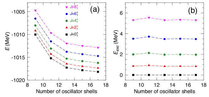
Figure 27: (a) Absolute and (b) excitation energies of the yrast band of ¹²⁰Cd calculated with a SCCM method -that includes PN-VAP+PNAMP wave functions along the axial quadrupole degree of freedom ($\beta_{2}$), using Gogny D1S- as a function of the number of major spherical harmonic oscillator shells included in the working basis.

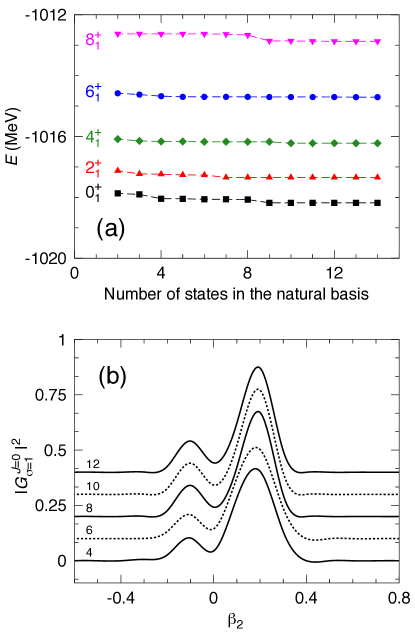
Figure 28: (a) Absolute energies of the yrast band of ¹²⁰Cd calculated with a SCCM method -that includes PN-VAP+PNAMP wave functions along the axial quadrupole degree of freedom ($\beta_{2}$), using Gogny D1S- as a function of the number states in the natural basis. (b) Collective wave function of the ground state, $0^{+}_{1}$, computed for different sizes of the natural basis (4, 6, 8, 10, 12). Curves are shifted for a better visualization.

We now review the multiple applications of the SCCM methods with Gogny EDFs that have been reported in recent years. Most of these studies have been focused on the calculation of bulk properties (masses, radii, etc.), excitation energies and electromagnetic properties (transition probabilities and moments) at low excitation energy. These quantities can be directly compared to experimental data and/or can give actual predictions for not-yet-measured nuclei. Moreover, apart from these observables, potential energy surfaces, Nilsson-like levels, occupation numbers and/or collective wave functions can be computed. These non-observable quantities provide a meaningful interpretation of the data in terms of the underlying shell structure, shapes, etc.. Most of these applications have their equivalent versions with Skyrme and RMF energy density functionals. In most of the cases, the three EDF provide similar results and global trends. As mentioned several times throughout the paper, we will restrict ourselves to review only the results obtained with Gogny interactions.

6.3.1 Global and local studies of BMF correlation energies

SCCM methods are based on the variational principle. The increase of complexity of the many-body states from purely mean-field (HFB-like) wave functions to symmetry restored and configuration mixing states is a way of getting closer and closer to the exact solution of the many-body problem. Therefore, including BMF correlations is essential to give a reliable theoretical description of the system. These correlations depend on the breaking and restoration of the symmetries of mean-field states, and the amount and relevance of the collective coordinates explored with the GCM method. Primarily, SCCM methods are designed to provide the best approach to the ground state energy. In fact, ground state correlations energies have been globally studied in Gogny EDFs with two kind of axial SCCM calculations, namely, parity projection plus GCM along the octupole degree of freedom [29, 37], and particle number and angular momentum projection plus GCM along the quadrupole degree of freedom [46]. In the latter case, the ground state correlation energies provided by the different BMF approaches used in a SCCM calculation are depicted for the nucleus ¹⁰⁸Pd in Fig. 29 as an example. This calculation has been extended to a wide range of even-even nuclei and D1S and D1M parametrizations as in Fig. 30 [46]. Here, we notice first the similar BMF correlation energies obtained with the two parametrizations. Moreover, we identify the order of magnitude of the different BMF correlation energies and the shell effects. These shell effects are rather prominent in PNAMP and GCM approximations. Hence, the energy gain is larger in mid-shell nuclei and negligible near magic nuclei when the rotational symmetry is restored (PNAMP), and the opposite happens when the quadrupole shape mixing is performed (GCM). Total BMF ground state correlation energies range from 4-8 MeV, having $\sim 6$ MeV in most of the cases for this kind of SCCM calculation.

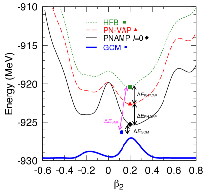
Figure 29: Potential energy surfaces as a function of the axial quadrupole deformation calculated with HFB (green dotted line), PN-VAP (red dashed line), and PNAMP (thin black continuous line) approximations for 108Pd with the Gogny D1S parametrization. The square, triangle, and diamond represent the minima of each surface. The blue dot corresponds to the full SCCM energy and the blue line represent the ground state collective wave function normalize to 1. The arrows point out the energy gain between the different BMF approaches.

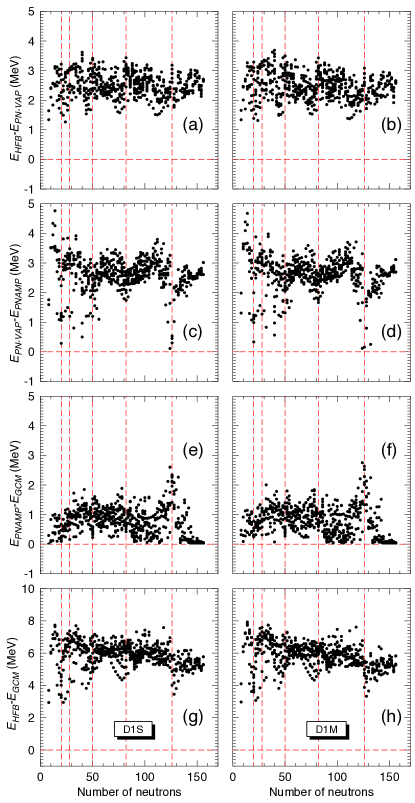
Figure 30: Gain in total energy as a function of the number of neutrons obtained by including BMF effects depicted in Fig. 29. Dashed vertical lines represent the neutron magic numbers 20, 28, 50, 82, and 126. Left and right columns correspond to Gogny D1S and D1M parametrizations, respectively. Figure taken from Ref. [46]

Similarly, BMF ground state correlation energies obtained by parity breaking, and parity projection plus octupole shape mixing are shown in Fig. 31 for Gogny D1M, although D1S and D1N parametrizations give almost the same results [37]. These energy gains are all defined with respect to the parity symmetric HFB ground state. In panel (a) only a few nuclei in the Ra, Ba and Zr regions show a non-zero correlation energy that never exceeds 1.2 MeV. These are the regions where a larger energy gain is also obtained when parity projection and octupole shape mixing is performed (panel (b)). The GCM correlation energy can be as large as 2.5 MeV. In the rest of the nuclei studied, the correlation energy is smaller, typically of the order of 1 MeV. Even though the computational cost compared to more traditional fits is much larger, BMF ground state correlation energies computed with SCCM methods should be taken into account in the future as it is clearly shown in Fig. 32 [46]. Here, the difference between the experimental and theoretical values for total energies are plotted both for mean-field (HFB) and the SCCM calculations with the Gogny D1M EDF. This parametrization already takes into account quadrupole shape mixings within the 5DCH in the fitting protocol. Therefore, the mean-field results are under-bound except for very few closed-shell nuclei (Fig. 32(a)). This effect is partially corrected with the inclusion of BMF ground state correlation energies (Fig. 32(b)). However, these corrections tend to overestimate (in average) the total energies. In addition, shell effects are very noticeable around the magic numbers in the mean-field approach and this drawback is not totally washed out with these SCCM calculations.

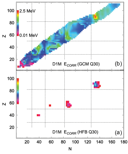
Figure 31: Octupole correlation energy gain as compared to HFB results preserving reflection symmetry. (a) the HFB correlation energy gained by breaking reflection symmetry; and, (b) the parity projection plus octupole GCM correlation energy. Horizontal and vertical dotted lines correspond to magic proton and neutron numbers. Figure adapted from Ref. [37].

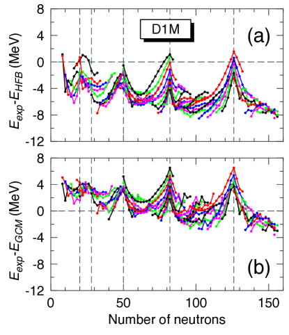
Figure 32: Difference between the experimental total energies (taken from Ref. [313]) and (a) HFB; and, (b) GCM total energies calculated with an axial SCCM method (including PNAMP and axial quadrupole shape mixing) with the D1M parametrization. Lines connect isotopic chains starting from $Z=10$. Black, red, blue, magenta, and green lines represent isotopic chains with $Z$ = x0, x2, x4, x6, and x8, where x = 1,2,…, etc. Dashed vertical lines mark the neutron magic numbers 20, 28, 50, 82, and 126. Figure adapted from Ref. [46].

Apart from the effect on total energies, axial SCCM calculations are well suited to study globally the performance of the method to reproduce other spectroscopic observables like $2^{+}$ (Fig. 33) or octupole excitation energies (Fig. 34). The overall trends of the experimental excitation energies are well reproduced with this kind of calculations although there are local discrepancies, and most importantly, the theoretical energies are too high in general. The origin of this stretching of the excitation energies could be mainly the lack of BFM correlations in the excited states. SCCM methods using axial and time-reversal symmetry conserving (TRSC) intrinsic wave functions to build the GCM basis explore variationally better ground states than excited states. Therefore, ground states calculated in this manner are closer (better converged from the variational point of view) to their exact values than the excited states that are still too above their exact values. These differences provoke the stretching of the theoretical spectra and the poor quantitative agreement with the experimental data shown in Figs. 33 and 34.

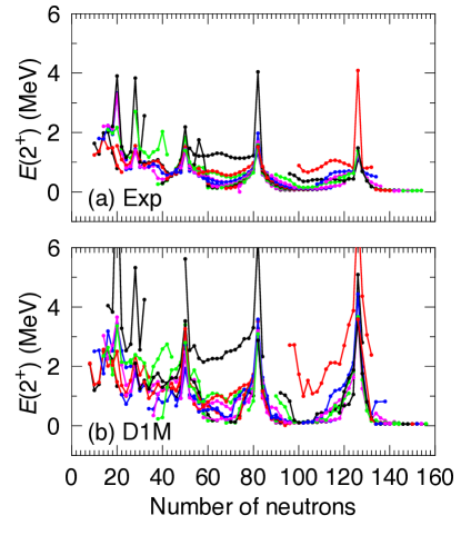
Figure 33: $2^{+}_{1}$ excitation energies for (a) experimental data (taken from Ref. [314]); and (b) an axial SCCM method (including PNAMP and axial quadrupole shape mixing) with the D1M parametrization. Lines connect isotopic chains starting from $Z=10$. The color code is the same as in Fig. 32. Figure adapted from Ref. [46].

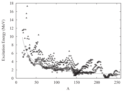
Figure 34: Octupole excitation energies as a function of mass number $A$ calculated with an axial SCCM method (including parity projection and axial octupole shape mixing) with the D1S parametrization. Circles: experiment; triangles: theory. Figure taken from Ref. [29].

Several improvements can be proposed to correct this drawback and have more predictive calculations at a quantitative level, for example, the inclusion of multi-quasiparticle intrinsic states. However, within the SCCM framework, where the symmetry restorations and configuration mixings are performed on top of quasiparticle vacua, the solution is to explore more collective degrees of freedom, in particular, triaxial deformations and intrinsically rotating states (cranking). In fact, excited states are particularly sensitive to the addition of cranking states [232, 235, 234, 315]. This procedure has also the convenient property of leaving unaltered the ground state. These effects are analyzed in Fig. 35. Here, the results of three different SCCM calculations with increasing complexity in the magnesium isotopic chain are shown. The simplest case corresponds to an axial SCCM method that includes PNAMP and axial quadrupole shape mixing, the intermediate case includes additionally static triaxial shapes, and cranking states (time-reversal symmetry breaking) are added to the previous ones in the most involved calculation. Therefore, the collective coordinates are the quadrupole deformation parameters, $(\beta_{2},\gamma)$, and the cranking intrinsic angular momentum, $J_{c}$ (see Fig. 22 for an example of states included in ³²Mg). Obviously, the cranking angular momentum is $J_{c}=0$ in the two first approaches, and the angle is only $\gamma=0^{\circ},180^{\circ}$ in the axial case. Fig. 35(a) shows the energy gain in the ground state by including static triaxial shapes to the ones used in the axial calculation. Since the method is based on the variational principle, this gain is always positive. Depending on the nucleus, the energy difference can be as large (small) as 1.4 MeV (0.1 MeV). More interestingly, the ground state correlations obtained by including the cranking states is very small ($<0.1$ MeV) revealing that the ground state energy is almost insensitive to this degree of freedom. However, we observe in Fig. 35(b) that this is not the case for excited states. Here, a similar qualitative behavior along the isotopic chain is obtained for the three calculations and also for the experimental data. However, the axial results are systematically above the triaxial values and the latter above the triaxial-plus-cranking. The stretching of the spectrum found in the axial and triaxial approximations is due to a privileged variational exploration of the ground state when the time-reversal symmetry is conserved. Then, the small compression of the energies in the triaxial approach is explained mainly by the possibility of $K$-mixing for states with $J\neq 0$. The larger compression of the spectrum given by the triaxial-plus-cranking method is due to a better variational exploration of the excited states since the ground state energies remain practically the same as the ones obtained with the triaxial approach (see Fig. 35(a)). Finally, the quantitative agreement with the experimental data reached with the most sophisticated SCCM method is excellent in this particular example.

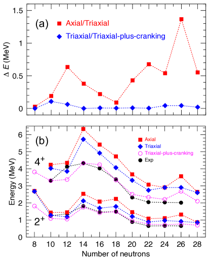
Figure 35: (a) Energy differences between the SCCM ground state energies in the magnesium isotopic chain computed with: axial and triaxial $J_{c}=0$ shapes (red squares); triaxial $J_{c}=0$ and triaxial-plus-cranking $J_{c}=0,2$ states (blue diamonds). (b) Experimental and SCCM excitation energies for the first $2^{+}$ and $4^{+}$ states in the magnesium isotopic chain. Data points are taken from Refs. [316, 317, 318, 319, 320, 321, 322]. Theoretical values are obtained with the D1S parametrization. Figure adapted from Ref. [235].

This method cannot be used to improve the description of $0^{+}$ excited states within the SCCM framework. For these cases, simultaneous quadrupole shape and pairing fluctuations mixing can be performed. This SCCM method has been implemented in Refs. [219, 220] with axial symmetric intrinsic wave functions and the quadrupole deformation ($\beta_{2}$) and the particle number fluctuations $(\Delta N^{2})$ as collective coordinates. This degree of freedom introduces mean-field states with different values of the pairing gap. The comparison between the results obtained only with quadrupole shape mixing (one-dimensional GCM calculations, 1D) and those obtained with adding $(\Delta N^{2})$ (2D calculations) reveal that the latter method produces in general a more compressed spectrum than the former. In Fig. 36 1D and 2D calculations for ^50-54Ca isotopes are shown as an example. Again, this effect is produced by a better variational exploration of the excited states. Particularly, the $0^{+}$ excitation energies can be pushed down improving their comparison with the experimental data as it is plotted in Fig. 37. Nevertheless, this compression is not large enough to reproduce the experimental values. This is an indication that some of the low-lying $0^{+}$ excited states correspond to explicit quasiparticle excitations rather than having a collective character. However, these states are out of the present SCCM methods with Gogny EDFs.

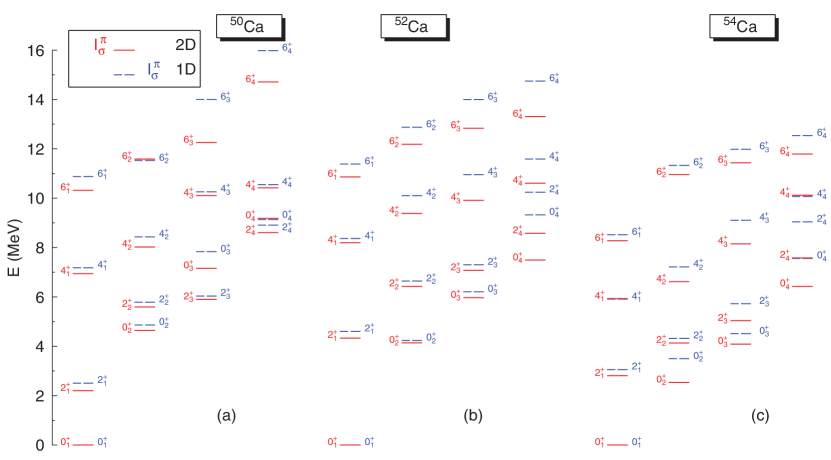
Figure 36: Spectra of ⁵⁰Ca, ⁵²Ca, and ⁵⁴Ca computed with two SCCM approximations, namely, including axial quadrupole shape mixing (1D) and adding particle number fluctuations (2D). Gogny In both cases . Figure taken from Ref. [220].

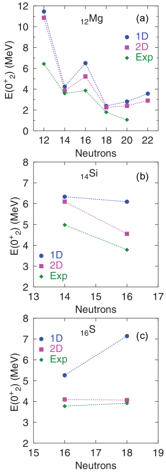
Figure 37: Excitation energies of the $0^{+}_{2}$ states in (a) Mg, (b) Si, and (c) S isotopes. Theoretical values are calculated as in Fig. 36 and experimental data are taken from Ref. [320]. Figure taken from Ref. [220].

6.3.2 Shape evolution/mixing/coexistence

Most of SCCM methods considers the lowest multipole (quadrupole and, to a lesser extent, octupole) intrinsic deformations as the basic collective coordinates. Therefore, this is the perfect framework to study, within a microscopic theory, the nuclear shape and its related phenomena (shape evolution in isotopic/isotonic chains, shape mixing and shape coexistence in a single nucleus). A complete analysis of the shape of a nucleus usually starts with the evaluation of mean-field (HFB) and/or particle number projected potential energy surfaces (PES) defined along the deformations of the system. The structure of the PES, i.e., the number of minima, their location, depth and width, already provides an overall view of the character of the nucleus in question. Moreover, the shape of the PES can be related to an underlying shell structure given by self-consistent Nilsson-like orbits. For example, the minima appear at deformations where the Fermi level crosses a gap in these single particle energies. However, SCCM methods go beyond these mean-field analyses and the theoretical predictions for excitation energies and electromagnetic properties can be directly compared to experimental data. Moreover, the most probable intrinsic shapes can be also obtained for each individual state within the nucleus by computing the collective wave functions.

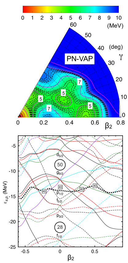
Figure 38: (a) Particle number projected (PN-VAP) potential energy surface -normalized to their absolute minima respectively- calculated for ⁸⁰Zr using the Gogny D1S interaction. Contour lines are separated by 0.2 MeV (dashed) and 1 MeV (continuous). (b) Single particle energies for neutrons as a function of the quadrupole deformation $\beta_{2}$. The Fermi level is represented by a thick dotted line. Figure adapted from Ref. [323].

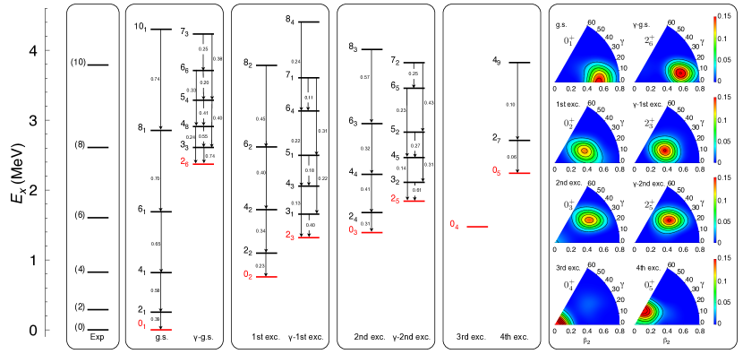
Figure 39: Left panel: Experimental and theoretical (with Gogny D1S) spectra for ⁸⁰Zr. $B(E2)$ values are given in $e^{2}b^{2}$. Right panel: Collective wave functions for the band heads of the bands. Figure taken from Ref. [323].

To illustrate the steps described above, we analyze the nucleus ⁸⁰Zr following Ref. [323]. In Fig. 38(a) the PES calculated with the PN-VAP method along the triaxial $(\beta_{2},\gamma)$ plane is plotted. Here, we observe several minima (spherical, axial prolate, axial oblate, triaxial) that could indicate the appearance of shape coexistence and/or shape mixing in this isotope. The origin of these minima in terms of the underlying shell structure is shown in Fig. 38(b) where the single-particle energies (s.p.e.) computed for this nucleus are plotted along the axial quadrupole deformation. Hence, the Fermi level crosses some gaps in these s.p.e. at the position of the minima obtained in the PES. These gaps are formed by the $pf$ and $g_{9/2}$ spherical shells (around the spherical point $\beta_{2}=0$) and by the evolution of these orbits whenever the quadrupole deformation is increased.

The final results after performing the particle number and angular momentum projection, and the quadrupole shape mixing (axial and non-axial), are shown in Fig. 39. Several bands are found in the theoretical spectrum. The character of these bands can be primarily characterized by their level spacing and electromagnetic properties ($B(E2)$ and spectroscopic quadrupole moments). For example, the ground state, first excited and second excited bands are rotational bands with side bands with a $\gamma$-band character associated to them. Experimentally, only some ground state band levels have been measured and they also indicate a rotational behavior.

As mentioned above, SCCM methods provide a very useful theoretical tool to identify the character of each state, namely, the collective wave functions (c.w.f.’s). These are represented in the right panel of Fig. 39 only for the band-head states since the rest of the states belonging to the same band show similar c.w.f.’s as their corresponding band-heads. We observe that the most relevant shapes in the ground state band are located at an axial prolate deformation, the second and third bands are triaxial deformed, and the $0^{+}_{4}$ and $0^{+}_{5}$ are spherical and slightly axial oblate deformed respectively. Hence, these states are related to the minima found in the PN-VAP PES and the reordering of the energy is mainly due to the correlations obtained by the angular momentum restoration of the system. Moreover, the c.w.f.’s do not show mixing between these minima and, therefore, this nucleus is an example of shape coexistence but not of shape mixing.

Shapes of both individual nuclei and systematics along isotopic chains have been thoroughly studied with SCCM methods with Gogny EDFs. First applications were done without particle number projection and assuming only the axial quadrupole deformation as the collective coordinate. Nevertheless, a good quantitative agreement was found in the description of normal deformed and superdeformed bands in ³²S [222], the shape evolution in $N=20$ and $N=28$ isotones and magnesium isotopes [221, 286, 223, 124], and the shape coexistence in neutron deficient lead isotopes [224]. In these works, intrinsic HFB instead of PN-VAP states were used. As mentioned above, the use of PN-VAP and simultaneous particle number and angular momentum restoration with Gogny EDFs was then implemented in Ref. [216], assuming again axial symmetry. The shape evolution of cadmium isotopes in the whole $N=50-82$ shell was well reproduced with these calculations, including the anomalous behavior of the $2^{+}$ excited state in the nucleus ¹²⁸Cd [324]. Moreover, the transition from spherical (U(5) symmetry) to axial prolate (SU(3) symmetry) shapes in neodymium and samarium isotopes, and its interpretation as a quantum phase transition (with X(5) as the critical symmetry), was also analyzed with axial SCCM calculations [325].

A breakthrough in the range of applicability of SCCM methods with Gogny interactions to study nuclear shapes was the inclusion of the quadrupole triaxial deformation as a collective coordinate [226]. At the same time, the access to high performance computing facilities has allowed the calculations of systematics along isotopic/isotonic chains within this formalism. A paradigmatic example is the study of the structure of krypton isotopes from neutron deficient to neutron rich nuclei [326]. Potential energy surfaces computed with Gogny D1S interaction in the $(\beta_{2},\gamma)$ plane reveal a rather involved shape evolution as it is shown in Fig. 40. The semi-magic nucleus ⁸⁶Kr is spherical -as expected- and their closest neighbors are slightly prolate deformed (^82-84,88-90Kr). Adding more neutrons above $N=50$ results in the appearance of an oblate minimum (^94-96Kr) and a potential shape coexistence (oblate-prolate) in ⁹⁸Kr. Clear candidates for shape coexistence are also obtained in the neutron deficient part where several nuclei show two distinct minima in their PES (^72-78Kr).

The shape evolution obtained after applying the full SCCM method can be seen in Fig. 41 where the ground state collective wave functions are represented. A clear transition from oblate to triaxial-prolate states is observed from ^70-72Kr to ^76-78Kr with the nucleus ⁷⁴Kr being the transitional isotope. In this case, the ground state c.w.f. is an example of shape mixing along the $\gamma$ degree of freedom. Around the spherical $N=50$ isotope, nuclei are less deformed as it could inferred from the PES (^82-84Kr and ^88-90Kr). Then, the deformation increases again towards oblate deformed nuclei (^94-98Kr).

Apart from this analysis, the results obtained with the SCCM can be compared to the experimental data as it is plotted in Fig. 42. The agreement is rather good except for the region around $N=50$ where explicit quasiparticle excitations will play a relevant role to account for these excited states. Furthermore, the improvement achieved by the inclusion of the triaxial degree of freedom with respect to purely axial SCCM calculations is also represented in Fig. 42.

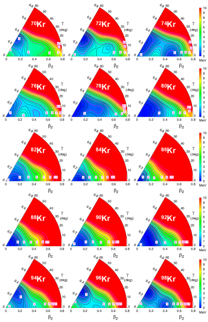
Figure 40: Potential energy surfaces in the triaxial plane calculated with PN-VAP method and the Gogny D1S interaction for Kr isotopes. Figure adapted from Ref. [326].

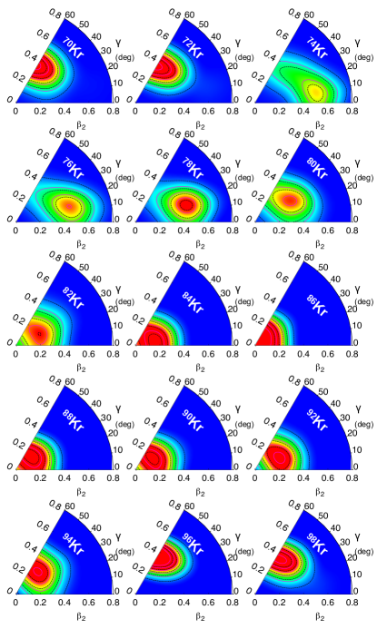
Figure 41: Collective wave functions for the ground states calculated with the SCCM method and the Gogny D1S interaction for Kr isotopes. Figure adapted from Ref. [326].

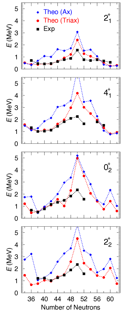
Figure 42: Excitation energies along the krypton isotopic chain ^70-98Kr for (a) $2^{+}_{1}$, (b) $4^{+}_{1}$, (c) $0^{+}_{2}$, and, (d) $2^{+}_{2}$ states. Black boxes, blue diamonds, and red bullets represent the experimental values (taken from Ref. [320]), and the results of SCCM axial and SCCM triaxial calculations, respectively. Figure taken from Ref. [326].

Hence, this kind of SCCM calculations with Gogny EDFs including particle number and angular momentum projection and triaxial quadrupole shape mixing have been extensively used recently in collaboration with experimental groups. For example, the role of triaxiality in the shape evolution, shape mixing and/or shape coexistence has been studied in ⁴²Ca [327, 328], neutron rich Zn [329], Ge [330, 331], Se [332], Kr [303], Mo [333], Os [334] and Pt [335] isotopes, comparing the most recent experimental data with theoretical predictions provided not only by Gogny SCCM methods but also by large scale shell model calculations, 5DCH approaches, and/or other SCCM methods with Skyrme functionals.

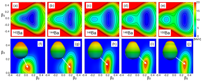
Figure 43: (a)-(e) Potential energy surfaces in the $(\beta_{2},\beta_{3})$ plane for the Ba isotopic chain for $N=86-94$. (f)-(j) Calculated collective wave functions of the ground states ($0^{+}_{1}$) are represented for $\beta_{3}>0$. To better visualize the shape of the isotopes, the surface that joins the points with constant spatial density is also shown for each isotope. These densities are computed with the HFB wave functions that correspond to the maximum of each collective wave function (see the arrows). Figure taken from Ref. [336].

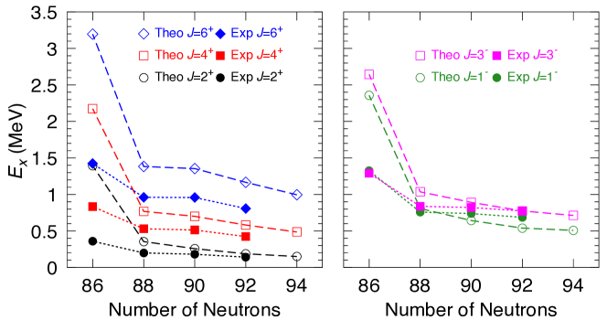
Figure 44: Experimental (filled symbols) and theoretical (open symbols) energy spectra in the Ba isotopic chain. Positive-parity states are grouped in panel (a) while the negative-parity ones are grouped in panel (b). Figure taken from Ref. [336].

On the other hand, SCCM calculations including particle number, parity and angular momentum projection and both axial quadrupole and octupole shape mixing have been also applied to study the interplay between quadrupole and octupole degrees of freedom, in particular, in neutron rich barium isotopes [231, 100, 336]. The mean-field PES and the ground state collective wave functions in the $(\beta_{2},\beta_{3})$ plane are represented for ^142-150Ba nuclei in Fig. 43. Here, we see the increase of quadrupole deformation whenever the number of neutrons departs from $N=82$. More interestingly, we observe the appearance of a non-negligible octupole deformation in this region that remains even after carrying out the shape mixing. The comparison between the theoretical predictions and the experimental data is shown in Fig. 43 both for positive and negative parity states. The qualitative agreement with the experiment is rather good although the transition between less quadrupole deformed (¹⁴²Ba) to well-deformed states (^144-150Ba) is sharper in the theoretical results.

6.3.3 Shell closures

SCCM methods are also suited to analyze the appearance/degradation of magic numbers in exotic nuclei. This property is intimately linked to the previous section since closed-shell (open-shell) nuclei are spherical (deformed). From the experimental point of view, large values of the excitation energies, $E(2^{+}_{1})$, and small values of the reduced transition probabilities, $B(E2)$, indicate the presence of shell closures in even-even nuclei. The opposite is considered as fingerprints of a collective behavior typical from open-shell systems. SCCM methods have access to show the most relevant intrinsic shapes to build a given nuclear state (i.e., the collective wave function), and, on the other hand, the excitation energies and electromagnetic properties computed in the laboratory system. The latter can be directly compared to the experimental data.

First applications to the study of shell closures within this framework were also the ones referred above with angular momentum projection and axial quadrupole deformation mixing but without particle number projection [221, 286, 223, 124]. These calculations showed that $N=20$ and $N=28$ are not good magic numbers in ³²Mg, and ⁴⁴S, ⁴²Si and ⁴⁰Mg, respectively, since small excitation energies, large $B(E2)$ values and deformed ground state c.w.f.’s were predicted. These results were in qualitative agreement with the available experimental data.

Figure 45: Experimental (black bullets) and theoretical $2^{+}_{1}$ excitation energies for calcium isotopes. Calculations are performed with SCCM methods including particle number and angular momentum projection, and axial quadrupole shapes (red squares), axial and triaxial quadrupole shapes (blue diamonds) and axial and triaxial with and without cranking states (magenta circles). Gogny D1S is used.

The potential new shell closures at $N=32$ and $N=34$ in neutron rich calcium isotopes were studied with axial SCCM including particle number projection [216]. Again, a qualitative agreement with the experimental data was obtained for the $E(2^{+}_{1})$ and reduced transition probabilities in the Ca, Ti and Cr chains around this number of neutrons. These calculations forecast, apart from the well-known $N=28$ shell closure at ⁴⁸Ca, a $N=32$ robust shell closure in ⁵²Ca and a decrease of the $E(2^{+}_{1})$ excitation energy in $N=34$ (see Fig. 45). The latter prediction in the nucleus ⁵⁴Ca was confirmed experimentally later on [337]. Furthermore, Fig. 45 shows again the compression of the theoretical spectrum whenever triaxial and cranking states are included within the SCCM method (see also Fig. 35). In the most sophisticated case, the theoretical results are in a good quantitative agreement with the experimental values and anticipate a $N=40$ (spherical harmonic oscillator) shell closure in ⁶⁰Ca. In fact, the degradation of spherical harmonic oscillator shell closures has been also analyzed with SCCM methods with the Gogny interaction, e.g., in Zirconium isotopes ($Z=40$) [323, 304] and in neutron rich $N=40$ isotones (⁶⁶Fe, ⁶⁴Cr and, to a lesser extent, ⁶²Ti) [338].

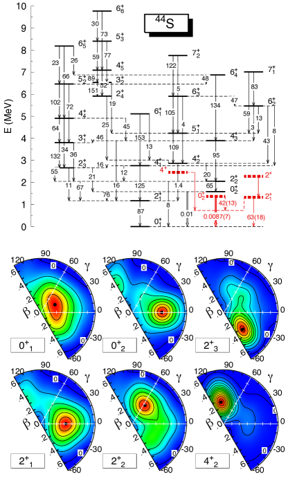
Figure 46: Top panel: Excitation energies, $B(E2)$ (in e²fm⁴) and $\rho^{2}(E0)$ for ⁴⁴S calculated with a SCCM method with Gogny D1S that includes static and cranking intrinsic states in the $(\beta_{2},\gamma)$ plane. Experimental data are shown as thick dashed lines. Bottom panel: Collective wave functions for the selected states shown in the legend. Figure adapted from Ref. [32].

Very recently, SCCM calculations including three sextants in the $(\beta_{2},\gamma)$ plane and states with different cranking frequency have been performed to study the structure of ⁴⁴S [32] and ⁴²Si [3]. In both cases deformed configurations have been found in the ground state, proving the degradation of $N=28$ magic number in these neutron rich nuclei. In addition, the inclusion of cranking states in the three sextants allows, on the one hand, an outstanding agreement with the experimental data, and, on the other hand, the description of isomeric states related to aligned states produced by rotations near the cranking axis [32, 3]. This is represented in Fig. 46 as an example. In the top panel, the theoretical spectrum shows a ground state band and a first excited band with $\Delta J=2$ and built on top of $0^{+}_{1}$ and $0^{+}_{2}$ states respectively. Additionally, three $\Delta J=1$ bands are obtained on top of $2^{+}_{3}$, $2^{+}_{4}$ and $4^{+}_{2}$ states. The band-head of the latter is very close in energy to the $4^{+}_{1}$ state but it has a very different character. This result is in a very good agreement with the most recent experimental data plotted in red. In the bottom panel of Fig. 46 the collective wave functions of the relevant states are shown to give a more detailed physical insight. Here, the ground state is found to be deformed and have a significant shape mixing along the triaxial degree of freedom. In addition, the $2^{+}_{1}$ and $0^{+}_{2}$ states are axial prolate deformed. On the whole, this is a fingerprint of the degradation of $N=28$ shell closure in this nucleus. A similar result was already obtained with Gogny SCCM triaxial calculations without cranking [339]. However, those time-reversal symmetry conserving calculations could not reproduce the low-lying $4^{+}_{2}$ state almost degenerated with the $4^{+}_{1}$ state since it corresponds to a less collective state peaked at a deformation close to the intrinsic (cranking) rotation axis. Thus, this state is considered as an aligned state with $K=4$ that is only obtained thanks to the inclusion of the cranking degree of freedom.

6.3.4 Lepton number violating processes

Symmetry conserving configuration mixing methods with Gogny EDFs can be also used to evaluate nuclear matrix elements of lepton number violating processes such as neutrinoless double beta decay ($0\nu\beta\beta$) [340, 341, 342, 343, 344]. This decay is the most promising process to disentangle the Majorana nature of the neutrino, its effective mass and the mass hierarchy [345, 346]. Here, an even-even nucleus decays into its even-even neighbor with two protons (neutrons) more (less). This process is energetically possible and is not hindered by single-beta decay in only very few cases across the nuclear chart. $2\nu\beta\beta$ decays, where two neutrinos are also emitted in the process, have been already observed with very long half-lives ($~{}10^{19-21}$ years), but the neutrinoless channel, the relevant one to study those properties of the neutrinos, has not been experimentally detected yet. In the most plausible scenario in which a light Majorana neutrino is exchanged in the $0\nu\beta\beta$ decay, the inverse of the half-life is [345]:

$$\left[T_{1/2}^{0\nu}(0_{i}^{+}\rightarrow 0_{f}^{+})\right]^{-1}=G_{0\nu}|M^{0\nu}|^{2}\left(\frac{\langle m_{\beta\beta}\rangle}{m_{e}}\right)^{2}$$ (171)

where $G_{0\nu}$ is a kinematic phase space factor, $m_{e}$ is the electron mass and $\langle m_{\beta\beta}\rangle$ is the effective Majorana neutrino mass. The nuclear physics part of this process is encoded in the so-called nuclear matrix element (NME), $M^{0\nu}$. Several nuclear structure methods have been used so far to calculate these NMEs (see Ref. [346] and references therein), namely, large scale shell model (SM), quasiparticle random phase approximation (QRPA), interacting boson model (IBM), projected Hartree-Fock-Bogoliubov (PHFB) and energy density functional methods (EDF).

In most of the cases, these NMEs are computed as the matrix elements between the $0^{+}$ ground states of the mother and granddaughter nuclei connected by the corresponding transition operator. This is the so-called closure approximation since it by-passes the virtual transitions to the intermediate states in the odd-odd nucleus. Therefore, SCCM methods with Gogny EDF, including particle number and angular momentum restoration, and axial quadrupole shape mixing, can be used to compute the ground states of the two neighboring nuclei involved in the process, and then, the corresponding transition matrix elements, as it is regularly done in electromagnetic decays.

The transition operator of this electroweak process is obtained assuming additionally a non-relativistic approach. Thus, the NMEs is given by the sum of Fermi (F), Gamow-Teller (GT) and tensor (T) terms [345], although the latter are normally neglected in Gogny EDF applications:

$$M^{0\nu}=-\left(\frac{g_{V}}{g_{A}}\right)^{2}M^{0\nu}_{F}+M^{0\nu}_{GT}$$ (172)

with $g_{V}=1$ and $g_{A}=1.25$ being the vector and axial coupling constants, and:

$$M^{0\nu}_{F/GT}=\langle 0^{+}_{f}|\hat{M}^{0\nu}_{F/GT}|0^{+}_{i}\rangle$$ (173)

with:

$$\hat{M}^{0\nu}_{F} = \left(\frac{g_{A}}{g_{V}}\right)^{2}\sum_{i<j}\hat{V}_{F}(r_{ij})\hat{\tau}^{(i)}_{-}\hat{\tau}^{(j)}_{-},$$ (174)

$$\hat{M}^{0\nu}_{GT} = \sum_{i<j}\hat{V}_{GT}(r_{ij})(\hat{\bm{\sigma}}^{(i)}\cdot\hat{\bm{\sigma}}^{(j)})\hat{\tau}^{(i)}_{-}\hat{\tau}^{(j)}_{-}$$ (175)

In these expressions, $\hat{\tau}_{-}$ is the isospin ladder operator that changes neutrons into protons and $\hat{\bm{\sigma}}$ are the Pauli matrices acting on the spin part of the wave functions. The so-called neutrino potentials $\hat{V}_{F/GT}$ depend on the relative distance between two nucleons (see Refs. [345, 346] and references therein for more details).

NMEs within the SCCM framework are computed in the following manner. Initial ($i$) and final ($f$) states correspond to the ground states given by Eq. 162 with $(J=0,\sigma=1)$, or, in their respective natural basis (Eq. 167):

$$|0^{+}_{i/f}\rangle=|\Psi^{0+}_{1,i/f}\rangle=\sum_{\Lambda_{i/f}}g^{0+}_{1,i/f}(\Lambda_{i/f})|\Lambda^{0+}_{i/f}\rangle$$ (176)

Then, each component of the NME is calculated using an expression similar to Eq. 169. Using the natural basis that corresponds to each nucleus, the NME is evaluated as [340]:

$$M^{0\nu}_{F/GT}=\sum_{\Lambda_{f}\Lambda_{i}}\sum_{\mathbf{q}_{f}\mathbf{q}_{i}}(g^{0+}_{1}(\Lambda_{f}))^{*}\left(\frac{u^{0+}_{\Lambda_{f}}(\mathbf{q}_{f})}{\sqrt{n^{0+}_{\Lambda_{f}}}}\right)^{*}\bar{M}^{0\nu}_{F/GT}(\mathbf{q}_{f},\mathbf{q}_{i})\left(\frac{u^{0+}_{\Lambda_{i}}(\mathbf{q}_{i})}{\sqrt{n^{0+}_{\Lambda_{i}}}}\right)g^{0+}_{1}(\Lambda_{i})$$ (177)

Here, the quantity $\bar{M}^{0\nu}_{F/GT}(\mathbf{q}_{f},\mathbf{q}_{i})=\langle\Phi^{0+}_{f}(\mathbf{q}_{f})|\hat{M}^{0\nu}_{F/GT}|\Phi^{0+}_{i}(\mathbf{q}_{i})\rangle$, where $|\Phi^{0+}_{i/f}(\mathbf{q}_{i/f})\rangle$ are projected states defined in Eq. 163, gives the dependence of the NMEs with the collective coordinates of the mother and daughter whenever is properly normalized:

$$M^{0\nu}_{F/GT}(\mathbf{q}_{f},\mathbf{q}_{i})=\frac{\bar{M}^{0\nu}_{F/GT}(\mathbf{q}_{f},\mathbf{q}_{i})}{\sqrt{\langle\Phi^{0+}_{i}(\mathbf{q}_{i})|\Phi^{0+}_{i}(\mathbf{q}_{i})\rangle\langle\Phi^{0+}_{f}(\mathbf{q}_{f})|\Phi^{0+}_{f}(\mathbf{q}_{f})\rangle}}$$ (178)

Therefore, the value of the NME can be understood as the convolution of the collective wave functions of initial and final states with the intensity of the NMEs as a function of the collective coordinates given in the previous expression.

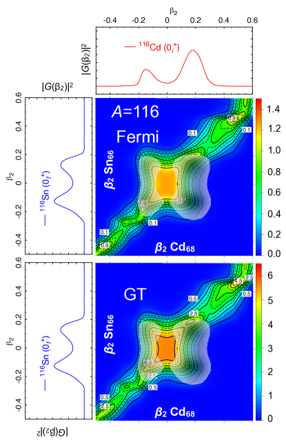
Figure 47: Contour plots: Strength of the Fermi and Gamow-Teller parts of $0\nu\beta\beta$ nuclear matrix elements as a function of the axial quadrupole deformation of the initial ¹¹⁶Cd and final ¹¹⁶Sn nuclei. Ground state collective wave functions for ¹¹⁶Cd (top) and ¹¹⁶Sn (left) nuclei. The shaded area shows the product of the two collective wave functions. Gogny D1S is used.

SCCM methods with Gogny EDFs are very well suited to study nuclear structure effects in the $0\nu\beta\beta$ NMEs. All of these calculations assume particle number and angular momentum restoration, and axial quadrupole shape mixing [226, 341, 342, 347, 344]. In Ref. [343] the fluctuations in the number of particles are also added as a collective coordinate. Thus, the role of deformation, pairing correlations and shell effects in the NMEs have been studied both in the actual candidates to detect $0\nu\beta\beta$ decays [226, 341, 343] as well as in virtual decays in isotopic chains [342, 344]. The latter studies are important to identify the origin of the discrepancies found in the NMEs computed with different many-body methods, in particular, between SCCM and SM calculations.

In general, SCCM calculations have shown that the strength of the NMEs is very much reduced when the deformations of the initial and final states are different. In fact, the decay is more probable between states with intrinsic spherical shapes. This is illustrated in Fig. 47 where the strength of the Fermi and GT parts in the decay of the nucleus ¹¹⁶Cd are plotted as a function of the axial quadrupole deformation of the mother (¹¹⁶Cd) and of the granddaughter (¹¹⁶Sn) (Eq. 178). The largest values correspond to the diagonal part of the figure, and, more specifically, to the area around the spherical shape. However, the final value of the NME considers the regions of these plots explored by the ground state collective wave functions of the initial and final nuclei. These are plotted on the top and on the left of Fig. 47 and the shaded areas correspond to the product of the two collective wave functions.

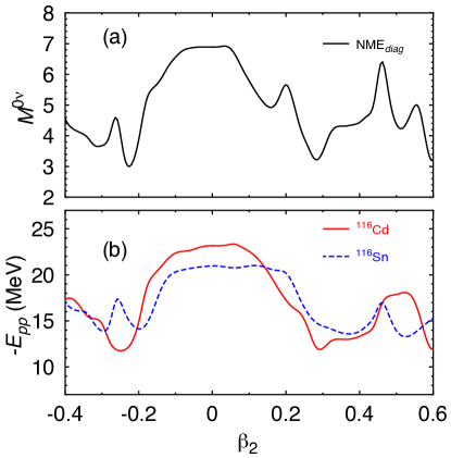
Figure 48: (a) Diagonal part of the $0\nu\beta\beta$ nuclear matrix elements, and, (b) pairing energies for ¹¹⁶Cd and ¹¹⁶Sn nuclei, as a function of the axial quadrupole deformation. Gogny D1S is used.

The other degree of freedom playing a major role in the $0\nu\beta\beta$ NMEs is the nuclear pairing. In Fig. 48 the pairing energies of the initial and final states as a function of the quadrupole deformation are represented as well as the diagonal part of the NMEs for the decay of ¹¹⁶Cd. Here, a clear correlation between these quantities are observed and the largest values of the NMEs are obtained at deformations where larger pairing energies are found. This effect was explicitly shown in Ref. [343], i.e., the increase of the NMEs with increasing the pairing content (proton-proton and neutron-neutron pairing) of the initial and final states. However, the actual values of the NMEs could be reduced by including two degrees of freedom that destroy like-particle pairing correlations, namely, higher seniority components (see, e.g., Ref. [344]) and proton-neutron pairing (see, e.g., Ref. [348]). This kind of states have not been included so far in SCCM Gogny EDF calculations.

Finally, the same formalism can be applied to the evaluation of NMEs of resonant neutrinoless double electron capture ($0\nu ee$) [349]. In this case, the SCCM calculations of the NMEs in the possible few candidates to detect this lepton number violating process predict much longer half-lives (of the order of $10^{31}$ years) than the $0\nu\beta\beta$ ones [350, 351].

6.3.5 Occupation numbers

Nuclear shell model (SM) and EDF methods are the most widely used frameworks to describe microscopically the nuclear structure. Thus, searching for connections between these formalisms are very useful due to their complementarity. SM works in the laboratory frame, diagonalizing effective nuclear interactions defined in valence spaces -normally assuming a core- and using Slater determinants -built upon a spherical mean-field- as the basis of the many-body Hilbert space [352]. On the other hand, EDF methods are defined in an intrinsic frame, i.e., tend to break most of the symmetries of the interaction at the mean-field level. Furthermore, these are no-core calculations and the number of major harmonic oscillator shells included is larger than in SM approaches. These aspects make SM and EDF states difficult to connect. Nevertheless, single-particle energies in the deformed basis with Nilsson-like plots are routinely found in EDF calculations to understand qualitatively the orbits that play a role for a given nucleus. In some cases, relevant deformed mean-field states have been studied in terms of the particle-hole structure in a spherical basis [353, 95].

A more quantitative way of analyzing the underlying shell structure of individual nuclear states within the SCCM framework has been recently proposed in Ref. [338]. It is based on computing the number of particles contained in each self-consistent spherical mean-field orbit when the states are defined with the SCCM ansatz (Eq. 162). These occupation numbers are not observables [354, 355] and are model dependent. However, they can provide a qualitative comparison of the internal structure of the SCCM states with SM states. On the other hand, they can also serve as a guidance for defining SM valence spaces because they reveal the importance of each spherical orbit in the description of, for example, rotational bands.

To calculate the occupation numbers of spherical orbits one needs to define first those single-particle levels. One reasonable choice is the canonical basis of the spherically-symmetric self-consistent mean-field solution of the nucleus under study. Thus, the operator associated to the number of particles occupying a given spherical orbit, $\alpha$, defined by the quantum numbers $(n_{\alpha}l_{\alpha}j_{\alpha})$ is:

$$\hat{n}_{\alpha}=\sum_{m_{j_{\alpha}}}a^{\dagger}_{n_{\alpha}l_{\alpha}j_{\alpha}m_{j_{\alpha}}}a_{n_{\alpha}l_{\alpha}j_{\alpha}m_{j_{\alpha}}}$$ (179)

These creation and annihilation single-particle operators $(a^{\dagger}_{\alpha},a_{\alpha})$ are obtained from the diagonalization of the density-matrix, $\rho^{sph}_{ab}$ [84]:

$$\rho^{sph}_{ab}=\langle\phi^{sph}|c^{\dagger}_{b}c_{a}|\phi^{sph}\rangle$$ (180)

where $|\phi^{sph}\rangle$ is the spherical quasiparticle vacuum and $(c^{\dagger}_{a},c_{a})$ are creation and annihilation single-particle operators that correspond to the arbitrary working basis used to define the HFB transformation [84]. As it is done in previous sections, the occupation numbers are now calculated as the expectation values of the operator defined in Eq. 179 between SCCM states, i.e., substituting $\hat{O}=\hat{n}_{\alpha}$ in Eq. 169. Moreover, the dependence of the occupation numbers along the collective coordinates can be computed as:

$$n^{J_{\sigma}\pi}_{\alpha}(\mathbf{q})=\frac{\langle\Phi^{J_{\sigma}\pi}(\mathbf{q})|\hat{n}_{\alpha}|\Phi^{J_{\sigma}\pi}(\mathbf{q})\rangle}{\langle\Phi^{J_{\sigma}\pi}(\mathbf{q})|\Phi^{J_{\sigma}\pi}(\mathbf{q})\rangle}$$ (181)

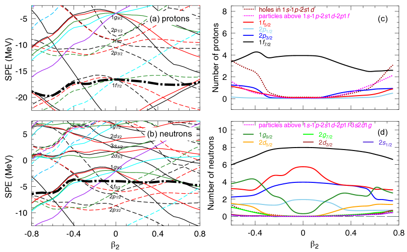
Figure 49: (a)-(b) Single-particle energies and (c)-(d) occupation numbers of spherical orbits as a function of the axial quadrupole deformation for protons and neutrons calculated for ⁶⁴Cr with the Gogny D1S interaction. Figure adapted from Ref. [338]

Thus, in the particular case where the collective coordinate is $\mathbf{q}=\beta_{2}$, Eq. 181 allows a quantitative evaluation of the number of particles occupying the different orbits along the quadrupole moment, improving the qualitative description that is usually given with the analysis of Nilsson-like plots. This is shown in Fig. 49 for the nucleus ⁶⁴Cr ($Z=24$, $N=40$) taken as an example of the performance of the method. In the left panel, the HFB single-particle energies and the Fermi level are represented for protons and neutrons. We observe that, around the spherical point, protons (neutrons) are expected to occupy up to the $f_{7/2}$ ($pf$-shell) orbits. Once the quadrupole deformation increases, some neutron levels coming from the $g_{9/2}$ and the $pf$-shell orbits cross the Fermi level, as well as one proton level coming from the $sd$-shell. The quantitative counterpart of this analysis is shown in the right panel. Here, we observe that the neutron $g_{9/2}$ orbit is clearly being filled in and the $f_{5/2}$ orbit is being emptied when the deformation departures from the spherical point.

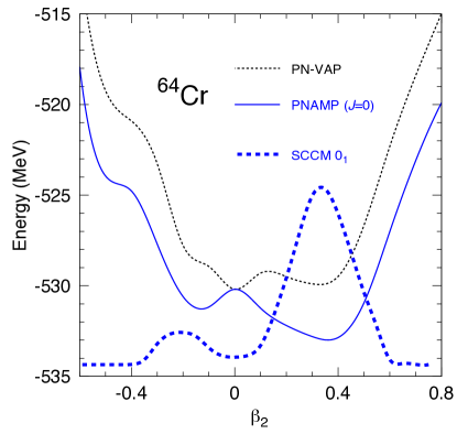
Figure 50: Potential energy surfaces as a function of the axial quadrupole deformation calculated for the nucleus ⁶⁴Cr with PN-VAP (dashed), and particle-number and angular momentum, $J=0$, projection (continuous) approaches. With the thick-dashed line, the ground state collective wave-function is shown. Gogny D1S is used. Figure adapted from Ref. [338].

The final values for the occupation numbers are given by the evaluation of Eq. 169 that includes the effect of the shape mixing. In Fig. 50 the particle number variation after projection (PN-VAP), the particle number and angular momentum ($J=0$) projection potential energy surfaces, and the ground state collective wave function are plotted. We see that, even though the $N=40$ spherical harmonic oscillator shell closure produces an absolute minimum in the PN-VAP PES, the angular momentum restoration and shape mixing produce that the deformed prolate configuration becomes the ground state. The occupation numbers computed in the ground state are represented in Fig. 51. To better visualize the relevant orbits needed to describe this deformed state, the difference between the occupation numbers provided by the SCCM method and the occupancies given by the HFB solution at the spherical point are plotted. Thus:

$$\Delta n^{J;\sigma}_{\alpha}=\langle\Phi^{J;\sigma}|\hat{n}_{\alpha}|\Phi^{J;\sigma}\rangle-\langle\phi^{sph}|\hat{n}_{\alpha}|\phi^{sph}\rangle$$ (182)

Positive (negative) values of $\Delta n^{J;\sigma}_{\alpha}$ mean particles (holes) in a given level $\alpha$ with respect to the filling in the spherical HFB configuration.

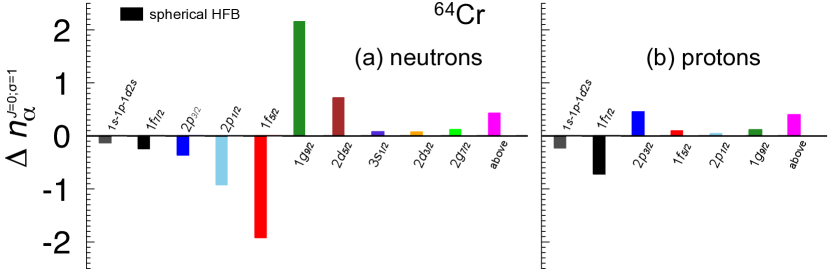
Figure 51: Difference between the occupation numbers of spherical orbits for the ground state of ⁶⁴Cr calculated with the SCCM method and the occupation numbers of those orbits in the spherical HFB configuration. Figure adapted from Ref. [338].

We observe that orbits below $1f_{7/2}$ are almost fully occupied and orbits above the neutron $sdg$ (proton $1g_{9/2}$) orbits have small (although non-negligible) occupancies. The neutron $pf$ ($1g_{9/2}$ and $2d_{5/2}$) orbits are depopulated (populated). Most of the depopulation of the neutron $pf$ shell comes from the $1f_{5/2}$ and $2p_{1/2}$ levels and, to a lesser extent, the $2p_{3/2}$ and $1f_{7/2}$ orbits. It is also interesting to see that $3s_{1/2}$, $2d_{3/2}$ and $2g_{7/2}$ are not very much populated in the ground state. Furthermore, the $1f_{7/2}$ orbit does not contain anymore the four valence protons as in the spherical case but it accommodates roughly one proton less, while the $2p_{3/2}$ and $2f_{5/2}$ starts to be slightly occupied. This analysis is in a rather good agreement with SM results and points out to the role of the $g_{9/2}$ neutron orbit in the onset of deformation in neutron rich $N=40$ isotopes (see Ref. [338] and references therein).

In summary, this method is a perfect tool to interpret the results of SCCM methods not only in terms of collective variables (with the collective wave functions) but also to study the underlying shell structure. Additionally, it allows a closer comparison with SM results, and, indirectly, with nucleon transfer/removal reaction experiments as it has been done in the case of ⁷⁶Ge and ⁷⁶Se [356].

7 Summary and future prospects

The success of the Gogny force in describing many different facets of nuclear structure along the years is a clear indication that it still represents a rock solid alternative for a microscopic description of the physics of the atomic nucleus in all regions of the nuclide chart with special emphasis on the interpretation of experimental findings.

For the years to come, one might think of several improvements to be made to the Gogny force. Some of them are minor, like including a finite range spin–orbit term or increasing the number of Gaussians. Some others require more work, like finding an operator based finite range replacement to the density dependent term, exploring the time-odd sector of the interaction or finding observables to fit a tensor term. The fitting protocol can also be improved as to take into account observables sensitive to proton-neutron pairing. Also, inclusion of beyond mean field effects in the fitting protocol should be a priority in the years to come. The exchange of ideas with the ab initio community could also seed some light on new forms of effective energy density functionals. Work in many of these considerations is already underway and hopefully we will witness some advances soon.

Concerning the improvement of the quantum mechanic many body methods to be used along with the Gogny force there are again minor developments that mostly involve the writing of new computer codes breaking all possible symmetries. In this category we could think of a triaxial QRPA code with the ability to compute also collective inertias exactly. New developments expanding beyond the use of a HO basis will be helpful to handle exotic shapes like to ones found in fission, the ones required to describe super-heavy elements or the accuracy needed for nuclear astrophysics. Also a proper handling of the continuum would be highly welcome to describe near drip-line physics and reactions from a more fundamental perspective.

Among the major improvements, a sound implementation of configuration interaction methods based on deformed intrinsic states which are subsequently projected to have the proper quantum numbers would be the main development. It will allow to treat consistently the physics of all kind of nuclei irrespective of their mass number and the collective character of the excitation under study. The challenge in this case is how to implement those methods for density dependent effective interactions. This will allow, among many other applications, to deal with odd mass systems at the same level of sophistication and applicability as the even-even case. Another major breakthrough would be the use of the Gogny force to analyze the time evolution of nuclear reactions using time dependent formalisms like TDHFB or TDGCM.

Appendix A Matrix elements of the Gogny force in the harmonic oscillator basis: basic ideas

The evaluation of matrix elements in mean field calculations with phenomenological effective interactions is of great relevance given the huge amount of them required, specially for heavy nuclei calculations. Therefore, it is highly desirable to find procedures to compute them in the quickest and most accurate possible way. In general, the matrix elements of two body operators are given as double three dimensional integrals (sixfold integrals) and different strategies have been used to reduce the complexity of their evaluation. A popular one in nuclear structure is to use contact interactions (as in the generic Skyrme case) to carry out analytically three of the integrals in order to reduce the sixfold integrals to threefold ones. Another strategy is to use interactions that factorize as products of the integration variables. This is the approach taken with the Gogny force, where the finite range central potential is given in terms of a Gaussian form factor

$$e^{-(\vec{r}_{1}-\vec{r}_{2})^{2}/\mu^{2}}=\prod_{i=1}^{3}e^{-(x_{i\,1}-x_{i\,2})^{2}/\mu^{2}}$$

By using basis states with the same factorization property it is possible to reduce the sixfold integration to the product of twofold integrals reducing thereby the amount of integrals to compute. The choice of a Gaussian form factor is advantageous for two additional reasons: First, it is intimately connected with the harmonic oscillator basis, as the Hermite polynomials are orthogonal with respect to a Gaussian weight and their generating functions are also Gaussians. As a consequence, the evaluation of the matrix elements in this basis can be carried out analytically. Second, it is possible to expand many smooth functions as a linear combination of tempered Gaussians (i.e. Gaussians with different widths) as it is common practice with the Coulomb and Yukawa potentials [357, 26] expanding enormously the range of applicability of the method.

An additional advantage of the harmonic oscillator basis is that, due to a nice property, it is possible to reduce the number of matrix elements to be computed in one dimension from $O(N^{2})$ to $O(N)$ where $N$ is the number of HO states [10, 11, 358].

For all the reasons above, calculations with the Gogny force are carried out in a harmonic oscillator basis. Depending on the underlying self-consistent symmetries of the calculation, spherical, axially symmetric or triaxial harmonic oscillator basis are used. The three representations are connected by means of unitary transformations [10, 359] and it is straightforward to go from one to another. In the following, we will illustrate the calculation of the matrix elements of a Gaussian form factor in the triaxial case, that is, assuming that the HO wave functions are factorized as the product of three one-dimensional HO states along each spatial direction $x$, $y$ and $z$

$$\varphi_{\alpha}(\vec{r})=\varphi_{a_{x}}(x)\varphi_{a_{y}}(y)\varphi_{a_{z}}(z)$$ (183)

The other two cases corresponding to spherical [11] ($r$, $\theta$ and $\varphi$ as spatial coordinates )and axial [85] ($r_{\perp}$, $\varphi$ and $z$) symmetries will not be considered here. The derivation presented here follows that of Ref [26] but taking into account the caveats discussed in [86] concerning the accuracy in the numerical evaluation of alternating sums.

The goal is to compute the matrix element of the two-body Gaussian interaction of the central part

$$I^{BB}_{abcd}=\int d\vec{r}_{1}d\vec{r}_{2}\varphi_{a}^{*}(\vec{r}_{1})\varphi_{b}^{*}(\vec{r}_{2})e^{-\frac{(\vec{r}_{1}-\vec{r}_{2})^{2}}{\mu^{2}}}\varphi_{c}(\vec{r}_{1})\varphi_{d}(\vec{r}_{2})$$ (184)

where $\varphi_{\alpha}(\vec{r})$ factorizes as $\varphi_{a_{x}}(x)\varphi_{a_{y}}(y)\varphi_{a_{z}}(z)$. The one-dimensional harmonic oscillator wave functions are given by the traditional expression in terms of the Hermite polynomials

$$\varphi_{n}(x;b)=\frac{1}{\sqrt{\sqrt{\pi}2^{n}n!b}}e^{-\frac{x^{2}}{2b^{2}}}H_{n}(x/b)$$ (185)

The generic matrix element of the Gaussian is then written as the product of three 1-D matrix elements

$$I_{abcd}^{BB}=\prod_{i=1}^{3}I_{a_{i}b_{i}c_{i}d_{i}}^{(i)}$$ (186)

where $I_{a_{i}b_{i}c_{i}d_{i}}^{(i)}$ is the two-dimensional integral

$$I_{a_{i}b_{i}c_{i}d_{i}}^{(i)}=\int dx_{1}dx_{2}\varphi_{{a_{i}}}(x_{1})\varphi_{{b_{i}}}(x_{2})e^{-\frac{(x_{1}-x_{2})^{2}}{\mu^{2}}}\varphi_{{c_{i}}}(x_{1})\varphi_{{d_{i}}}(x_{2})$$ (187)

The strategy to compute this integral is to use the following property of the harmonic oscillator wave functions [10, 11, 358]

$$\varphi_{n_{a}}(x)\varphi_{n_{c}}(x)=\frac{1}{b^{1/2}\pi^{1/4}}\sum_{n_{\mu}}\tau(n_{a}n_{c}n_{\mu})e^{-\frac{x^{2}}{2b^{2}}}\varphi_{n_{\mu}}(x)$$ (188)

where the sum on $n_{\mu}$ contains a finite number of terms ($|n_{a}-n_{c}|\leq n_{\mu}\leq n_{a}+n_{c}$) and the geometric coefficient $\tau(n_{a}n_{c}n_{\mu})$ is given by

$$\tau(n_{a},n_{b},n_{\mu})=\frac{\left(n_{a!}n_{b}!n_{\mu}!\right)^{1/2}}{(s-n_{\mu})!(s-n_{a})!(s-n_{b})!}\Delta_{n_{a}+n_{b},n_{\mu}}$$ (189)

with $s=\frac{1}{2}(n_{a}+n_{b}+n_{\mu})$ and

$$\Delta_{n,m}=\frac{1}{2}\left(1+(-)^{n+m}\right)$$ (190)

Preservation of the parity symmetry (expressed by the $\Delta$ symbol) guarantees that in all the non-zero coefficients the combinations in the denominator are integers and therefore the factorial makes sense. The result can be easily understood by noticing that, apart from the Gaussian factors, the 1D HO oscillator wave functions are polynomials and the product of two polynomials of degrees $n_{1}$ and $n_{2}$ can unambiguously be expressed as a linear combination of polynomials of degree $n_{1}+n_{2}$ at most. Using the above result the previous integral is expressed as

$$I_{abcd}^{(i)}=\frac{1}{b\sqrt{\pi}}\sum_{n_{\mu}n_{\nu}}\tau(n_{a}n_{c}n_{\mu})J(n_{b}n_{d}n_{\mu})$$ (191)

where

$$J(n_{b},n_{d},n_{\mu})=\frac{1}{b^{1/2}\pi^{1/4}}\int dx_{1}\varphi_{n_{\mu}}(x_{1})e^{-\frac{x_{1}^{2}}{2b^{2}}}\int dx_{2}e^{-\frac{(x_{1}-x_{2})^{2}}{\mu^{2}}}\varphi_{n_{b}}(x_{2})\varphi_{n_{d}}(x_{2})$$ (192)

To compute this set of coefficients there are essentially two alternatives: (a) to perform a transformation to the center of mass $(x_{1}+x_{2})/2$ and relative coordinate $x_{1}-x_{2}$ using Moshinsky coefficients or (b) to use the Parseval theorem of Fourier transforms to write the integral in momentum space as

$$\int d{k}F^{*}_{n_{\mu}}({k})\widetilde{G}_{n_{b}n_{d}}({k})$$ (193)

where $F_{n_{\mu}}(k)$ is the Fourier transform of $\varphi_{n_{\mu}}(x_{1})e^{-\frac{x_{1}^{2}}{2b^{2}}}$ and $\widetilde{G}_{n_{b},n_{d}}(k)$ is the Fourier transform of a convolution. Using these ideas we arrive to the final expression

$$J(n_{b},n_{d},n_{\mu})=\frac{\sqrt{2\pi}}{\sqrt{b\sqrt{\pi}}}\int dkF_{n_{\mu}}^{*}(k)E(k)G_{n_{b}n_{d}}(k)$$ (194)

where the corresponding quantities in momentum space are given by

$$F_{n_{\mu}}(k)=\mathcal{F}\left(\varphi_{n_{\mu}}(x_{1})e^{-\frac{x_{1}^{2}}{2b^{2}}}\right)={}\frac{b}{\sqrt{\sqrt{\pi}2^{n_{\mu}}n_{\mu}!b}}\frac{(-i)^{n_{\mu}}}{\sqrt{2}}\left(kb\right)^{n_{\mu}}e^{-(kb)^{2}/4}$$ (195)

for the Fourier transform of the 1-D HO wave function times a Gaussian,

$$E(k)=\mathcal{F}\left(e^{-x^{2}/\mu^{2}}\right)=\frac{\mu}{\sqrt{2}}e^{-(k\mu)^{2}/4}$$ (196)

for the Fourier transform of a Gaussian, and

$$G_{n_{b}n_{d}}(k) = \mathcal{F}\left(\varphi_{n_{b}}(x)\varphi_{n_{d}}(x)\right)={}\frac{n_{b}!n_{d}!(-i)^{n_{b}+n_{d}}}{\sqrt{\pi 2^{n_{b}+n_{d}+1}n_{b}!n_{d}!}}e^{-(kb)^{2}/4}$$

$$\times \sum_{p}\frac{(-2)^{p}}{p!(n_{b}-p)!(n_{d}-p)!}(kb)^{n_{b}+n_{d}-2p}$$

for the Fourier transform of the product of two 1-D harmonic oscillator wave functions. The momentum integral is straightforward and it imposes the selection rule $n_{\mu}+n_{b}+n_{d}=\textrm{even}=2s$. The final result is [86]

$$J(n_{b},n_{d},n_{\mu})=\frac{\mu}{b\sqrt{2\pi}}\frac{(-1)^{s+n_{\mu}}}{G^{s+1/2}}\left(\frac{n_{b!}n_{d}!}{n_{\mu}!}\right)^{1/2}\sum_{p}\frac{\Gamma(s-p+1/2)}{p!(n_{b}-p)!(n_{d}-p)!}\left(-G\right)^{p}$$ (198)

with the coefficient $G=1+\frac{\mu^{2}}{2b^{2}}$. The quantity $J(n_{b},n_{d},n_{\mu})$ can be written using hypergeometric series as

$$J(n_{b},n_{d},n_{\mu}) = \frac{\mu}{b\sqrt{2\pi}}\frac{(-1)^{s+n_{\mu}}}{G^{s+1/2}}\left(\frac{1}{n_{b!}n_{d}!n_{\mu}!}\right)^{1/2}\Gamma(s+1/2)$$

$$\times {}_{2}F_{1}(-n_{b},-n_{d},1/2-s;G)$$

The advantage of this result is the possibility to use the vast literature around hyper-geometric functions to find efficient and accurate ways to evaluate the coefficients. In the case $\mu=0$ it is even possible to find an explicit analytical expression for the above matrix element. In others, use of any of the 24 Gauss recursion relations is useful to simplify or make more accurate the evaluation of the $J$ coefficients.

The previous results can be used also to compute the matrix elements of a contact interaction $\delta(\vec{r}_{1}-\vec{r}_{2})$ given the relation between the delta function and a Gaussian of zero range

$$\delta(x_{1}-x_{2})=\lim_{\mu\rightarrow 0}\frac{1}{\sqrt{\pi}}\frac{e^{-(x_{1}-x_{2})^{2}/\mu^{2}}}{\mu}$$ (200)

It is also possible to use the above results to compute the matrix elements of the Coulomb interaction by using its expansion as a linear combination of tempered Gaussians [357, 26]

$$\frac{1}{|\overline{r}_{1}-\overline{r}_{2}|}=\frac{2}{\sqrt{\pi}}\int_{0}^{\infty}\frac{d\mu}{\mu^{2}}e^{-|\overline{r}_{1}-\overline{r}_{2}|^{2}/\mu^{2}}.$$ (201)

Using this expansion it is possible to express the matrix element of the Coulomb potential $I_{abcd}^{C}$ in terms of the integral of $I_{abcd}^{\mathrm{Gauss}}(\mu)$ with respect to $\mu$

$$I_{abcd}^{C}=\frac{2}{\sqrt{\pi}}\int_{0}^{\infty}\frac{d\mu}{\mu^{2}}I_{abcd}^{\mathrm{Gauss}}(\mu)$$ (202)

The only dependence on $\mu$ of $I^{\mathrm{Gauss}}$ is in the coefficients $J$ of Eq. (198). The integral on $\mu$ cannot be evaluated analytically, but an appropriate change of variables and the use of the Gauss-Legendre numerical integration allows for an accurate evaluation of the required integrals [26].

Using the same ideas of expanding in a linear combination of Gaussian functions it is also possible to compute the matrix elements of the Yukawa potential in this way [357, 360]

The evaluation of the matrix elements of the density dependent part of the interaction or the Slater approximation to the Coulomb exchange potential have necessarily to be carried out numerically. For this purpose, the Gauss-Hermite (or the appropriate one in the axially symmetric or spherical case) method is very handy at a moderate computational cost.

Appendix B Computer codes

To our knowledge, computer codes to carry out mean field and beyond mean field calculations with the Gogny force have been developed by several different groups: the Bruyères Le Châtel (BlC) group in France, the Madrid (Mad) group in Spain, several groups in Japan (see [361, 233] for two different implementations) and finally the collaborative effort around the HFBtho [362] and HFBodd [363] codes involving many scientists from different institutions. Of all the codes mentioned, only the HFBtho and HFBodd ones have been published [362, 363] in a journal or made publicly available. Therefore, after briefly discussing the published codes, we will be focusing in this section on the codes produced by the present authors which are available upon request to the authors.

The HFBtho is a computer code primarily developed to implement Skyrme HFB calculations in an axially symmetric transformed harmonic oscillator basis. The peculiarity of the transformed HO it that it allows for more flexibility in describing the asymptotic properties of the single particle wave functions. In the most recent version [362], the Gogny force has been incorporated as an option, but in the more traditional harmonic oscillator basis.

The HFBodd is a computer code that was born as an implementation of the HFB equation with the zero range Skyrme interaction. The recent versions of the code are flexible enough as to break all possible symmetries including simplex, reflection symmetry and time reversal. More recent versions also allow the calculation of Hamiltonian overlaps and projected energies for a variety of broken symmetries. The HFB amplitudes are expressed in a triaxial HO basis. In the last iteration of the code [363], the Gogny force has been incorporated as an option into the code.

The two codes above are written in fortran90 and include lots of computational tricks to improve performance like OpenMP or MPI for production in a parallel environment. However, in a single computer their performance is far from satisfactory in contrast with the computer codes developed by the present authors.

Along the years the authors have developed several computer codes in FORTRAN 77 to implement HFB and beyond calculations with the Gogny force. Let us first mention the family of codes preserving axial symmetry (but breaking reflection symmetry if required):

• HFBax is a HFB solver implementing all different terms of the Gogny force, including Coulomb exchange and Coulomb antipairing. It is based on an expansion on an axially symmetric harmonic oscillator basis with a single center. Thanks to it implementation of the evaluation of matrix elements using hypergeometric series (see Appendix A) it can go quite far in basis size without encountering any numerical instability (see [86]). It can even handle fission [23, 364] or even cluster emission [25] up to the scission point and beyond (two well separated fragments) without any problem. The method of choice to solve the HFB equation is a second order gradient method [29] that reduces substantially the iteration count. A procedure for an unattended minimization of the oscillator length parameters is also available.

• Atb is similar to HFBax but with the pecularity that time reversal invariance can be broken. This opens up the possibility to solve the HFB equations with full blocking and the self-consistent treatment of odd-A nuclei [81, 80] or even the study of high-K isomers [82] in super-heavy nuclei. One of the key elements of this code is the implementation of an orthogonality constraint to prevent the iterative solution of the HFB equation to always converge to the lowest lying solution for a given $K$ quantum numbers.

• HFBaxT represents the extension to finite temperature [31, 119, 120] of the HFBax code. It can also handle fission at finite temperature [120] as well as the calculation of level densities in the finite temperature framework.

• PNPax computes the particle number projected energy of a HFB wave function obtained with HFBax. It also allows for a search, in the spirit of the RVAP with the particle number fluctuation as variational parameter, of the lowest energy PNP solution.

• GCMax is a computer code to compute the Hamiltonian overlap between any two general HFB wave functions obtained from HFBax. This computed code together with an auxilliary program (HW) can be used to solve the Hill-Wheeler equation of the GCM procedure for axially symmetric wave functions. Applications to GCM calculations with the octupole degree of freedom as generating coordinate [29] or the quadrupole and octupole degree of freedom [47, 102] are common applications of this computer code.

A triaxial code breaking time reversal symmetry, but preserving simplex is also available. It is dubbed HFBTri and it can handle both even and odd number parity type of wave functions. Together with the possibility to break time reversal, the handling of odd number parity states opens up the opportunity to deal with odd mass nuclei using the HFB blocking procedure. The constraint in orthogonality is fully implemented as well as several other constraints on two body operators like $\langle\Delta N^{2}\rangle$ or $\langle\Delta J_{z}^{2}\rangle$. The method of choice to solve the HFB equation is a second order gradient method [29] that reduces substantially the iteration count. It shares with the HFBax the same protocols to compute the matrix elements and therefore rather large basis sizes up to 20 shells can be used.

Appendix C Overlaps of operators between HFB states: the Generalized Wick Theorem

In the implementation of symmetry restoration and/or configuration mixing the evaluation of overlaps of operators between arbitrary HFB states is required. This is so because the symmetry operators are exponentials of one body operators (which are part of the Lie algebra generating the HFB states) and therefore its action on arbitrary HFB states leads again to HFB states.

The evaluation of the overlaps is greatly simplified by using the Generalized Wick Theorem (GWT). The theorem, derived in many different ways [365, 366, 367, 368], states that generic overlaps of the form

$$\frac{\langle\Phi|\hat{O}|\Phi^{\prime}\rangle}{\langle\Phi|\Phi^{\prime}\rangle}$$ (203)

can always be written as the sum of all possible two-quasiparticle contractions

$$\frac{\langle\Phi|\beta_{\mu}\beta_{\nu}|\Phi^{\prime}\rangle}{\langle\Phi|\Phi^{\prime}\rangle} = C_{\mu\nu}$$ (204)

$$\frac{\langle\Phi|\beta_{\mu}\beta_{\nu}^{\dagger}|\Phi^{\prime}\rangle}{\langle\Phi|\Phi^{\prime}\rangle} = \delta_{\mu\nu}$$ (205)

$$\frac{\langle\Phi|\beta_{\mu}^{\dagger}\beta_{\nu}^{\dagger}|\Phi^{\prime}\rangle}{\langle\Phi|\Phi^{\prime}\rangle} = 0$$ (206)

In the above expressions $|\Phi\rangle$ and $|\Phi^{\prime}\rangle$ are arbitrary, non orthogonal, HFB wave functions with amplitudes $U$, $V$ and $U^{\prime}$, $V^{\prime}$ respectively and $\hat{O}$ is a general multi-body operator. Typically, the operator $\hat{O}$ is a linear combination of products of creation and annihilation quasiparticle operators belonging to a given HFB state. To simplify the results, we will assume that those quasiparticle operators are the ones associated to $|\Phi\rangle$. As an example, considering $\hat{O}$ to be a one-body operator we obtain

$$\frac{\langle\Phi|\hat{O}|\Phi^{\prime}\rangle}{\langle\Phi|\Phi^{\prime}\rangle} = \langle\Phi|\hat{O}|\Phi\rangle+\frac{1}{2}\sum_{munu}O^{20}_{\mu\mu}\frac{\langle\Phi|\beta_{\mu}\beta_{nu}|\Phi^{\prime}\rangle}{\langle\Phi|\Phi^{\prime}\rangle}$$

$$= \langle\Phi|\hat{O}|\Phi\rangle+\frac{1}{2}\sum_{munu}O^{20}_{\mu\mu}C_{\mu\nu}$$

The only non-trivial contraction required in the previous overlap is given in terms of the skew-symmetry matrix $C_{\mu\nu}$ which is the product of two matrices

$$C_{\mu\nu}=A^{-1}B$$ (208)

where $A=U^{\dagger}U^{\prime}+V^{\dagger}V^{\prime}$ and $B=U^{\dagger}V^{\prime}+V^{\dagger}U^{\prime}$. Using the GWT we can write, for instance, the non-trivial matrix element entering the evaluation of the Hamiltonian overlap as

$$\frac{\langle\Phi|\beta_{\mu}\beta_{\nu}\beta_{\sigma}\beta_{\rho}|\Phi^{\prime}\rangle}{\langle\Phi|\Phi^{\prime}\rangle}=C_{\mu\nu}C_{\sigma\rho}-C_{\mu\sigma}C_{\nu\rho}+C_{\mu\rho}C_{\nu\sigma}.$$ (209)

The overlap between the two HFB wave functions is given by the expression

$$\langle\Phi|\Phi^{\prime}\rangle=\pm\sqrt{\det A}.$$ (210)

The presence of the square root implies an indeterminacy in the sign that requires further consideration. The importance of the undetermined sign comes from the fact that the overlap is part of the integrand of the integrals characteristic of the symmetry restoration or configuration mixing methods. A wrong assignment of the sign can substantially change the value of the integral. The sign problem has been addressed in the past using different strategies

• Continuity: The wave function $|\Phi^{\prime}\rangle$ belongs to a dense set that includes $|\Phi\rangle$. By fixing the initial sign by $\langle\Phi|\Phi\rangle=1$, the one of $\langle\Phi|\Phi^{\prime}\rangle$ for a $|\Phi^{\prime}\rangle$ close to $|\Phi\rangle$ is fixed by continuity. The method is complemented by the knowledge of the derivative of the overlap with respect to some parameter $\alpha$ labeling the set of the $|\Phi^{\prime}\rangle$. However, the method requires an adaptive mesh to work in arbitrary situations.

• Time reversal invariant systems: in those cases where there is Kramer’s degeneracy the Bogoliubov amplitudes have a block structure that also renders the matrix $A$ as a block matrix with equal entries $\bar{A}$ in the diagonal. As a consequence the $\det A$ is given by a square $\det A=\det^{2}\bar{A}$ and therefore $\langle\Phi|\Phi^{\prime}\rangle=\det\bar{A}$.

• Neergard and Wüst method: Factoring out the matrices $U^{\dagger}$ and $U^{\prime}$ off the matrix $A$ we can express the overlap in terms of the determinant $\det(1+Z^{\dagger}Z^{\prime})$ where the skew symmetric matrices are simply given by $Z=VU^{-1}$. As shown in Ref. [369] the matrix $Z^{\dagger}Z^{\prime}$ has doubly degenerate eigenvalues and again $\det(1+Z^{\dagger}Z^{\prime})$ can be written as a square.

• Pfaffian method: Using techniques of fermion coherent states it is possible to compute the overlap of two arbitrary HFB states without any ambiguity in the sign [370]. The final results is expressed in terms of the Pfaffian of a skew-symmetric matrix. The Pfaffian of a skew-symmetrix matrix is defined in a similar fashion to the determinant of an arbitrary matrix and shares with the determinant many properties. An interesting property of the Pfaffian is the one connecting the Pfaffian with the square of a determinant. The numeric evaluation of the Pfaffian has a computational cost very similar to the one of the determinant and therefore it represents a very useful alternative to any of the methods mentioned above [371].

There are a couple of difficulties in the application of the GWT or overlap formulas in practical implementations. One has to do with the common situation where the occupancies $v_{k}^{2}$ of the HFB wave functions involved are close to one. In this case some of the expressions involving the inverse of the $U$ amplitudes are not well defined. This problem has been solved in the literature [205, 372, 373]. Also useful formulas to deal with unoccupied (and therefore irrelevant) states have been given. The other difficulty is connected with the situation where the overlap of the two HFB wave functions is zero and therefore the contractions of the GWT as given in Eq (204) are ill defined (in fact, divergent). This might be thought as an expectional situation but it is indeed common in PNP or in other similar contexts involving cranking wave functions [92, 374]. The consequences of this failure of the GWT have been discussed in many places [92, 202] in the context of EDFs and is still an unresolved aspect of the theory that has to be further clarified. If the overlap $\langle\Phi|\hat{O}|\Phi^{\prime}\rangle$ is still required, a way to compute it is going to a sort of canonical basis [375, 202] or use the Pfaffian technique as discussed in [368]. In the latter reference, a way to compute efficiently overlaps of multiquasiparticle excitations of the different HFB vacuums without the combinatorial explosion characteristic of the GWT has been considered. It is again based on the Pfaffian ideas and could represent a breakthrough in applications of the projected shell model of Hara and Sun [367].

Another practical aspect of the GWT has to do with the common situation when the two HFB wave functions are expanded on different single particle basis not spanning the same subspace of the whole Hilbert space. In this case, the formulas above have to modified to take into account this peculiarity. The idea is to formally enlarge both basis as to expand the same subspace but setting to zero the occupancy of the extended orbitals [205, 376, 368].

In applications involving statistical ensembles, where traces with a density matrix operator are used instead of mean values, it is still possible to used the ideas of the GWT in those cases where a given operator is multiplied by the exponential of an one body operator (a symmetry transformation or a Bogoliubov transformation operator). The corresponding expression is similar to the one of the GWT (linear combination of contractions) but the contractions are given by a different expression [377, 378].

Appendix D Abbreviations and acronyms

In the following table a list of abbreviations and acronyms used in the paper is given

5DCH	5D Collective Hamiltonian
AMP	Angular momentum projection
AM-PAV	Angular momentum PAV
AM-VAP	Angular momentum VAP
BCS	Bardeen Cooper Schrieffer
BHF	Bruckner HF
CHFB	Cranked Hartree Fock Bogoliubov
COM	Center of Mass
CSE	Collective Schrödinger equation
EDF	Energy density functional
EFA	Equal filling approximation
EOS	Equation of state
FTHFB	Finite temperature HFB
GCM	Generator coordinate method
GOA	Gaussian overlap approximation
HFB	Hartree Fock Bogoliubov
HF	Hartree Fock
HO	Harmonic Oscillator
HWG	Hill-Wheeler-Griffins
IBM	Interacting boson model
LN	Lipkin Nogami
PAV	Projection After Variation
PES	Potential energy surface
PLN	Projected LN
PNAMP	Particle number AMP
PN-PAV	Particle number PAV
PNP	Particle Number Projection
PN-VAP	Particle number VAP
PPNAMP	Parity PNAMP
QRPA	Quasiparticle RPA
RMF	Relativistic Mean Field
RPA	Random Phase Approximation
R-PN-VAP	Restricted PN-VAP
RVAP	Restricted VAP
SCCM	Symmetry conserving configuration mixing
SCK2	Self-consistent Kamlah 2
TRSC	Time reversal symmetry conserving
TR	Time reversal
VAP	Variation After Projection

The parametrizations of the Gogny force discussed in Sec. 2 are also listed here for a compilation:

• Traditional D1 family: D1, D1’, D1S, D1N, D1M, D1P, DS280, D1M^∗

• New D2 family: D2

• Including tensor term: D1ST, D1MT, D1ST2a, D1ST2b, D1MT2c, GT2

• Similar to Gogny: SEI

References

- [1] J. F. Berger, J. P. Blaizot, D. Bouche, P. Chaix, J. P. Delaroche, M. Dupuis, M. Girod, J. Gogny, B. Grammaticos, D. Iracane, J. Lachkar, F. Mariotte, N. Pillet, and N. Van Giai. Daniel gogny. The European Physical Journal A, 53(10):214, Oct 2017.
- [2] S. Péru and M. Martini. Mean field based calculations with the gogny force: Some theoretical tools to explore the nuclear structure. The European Physical Journal A, 50(5):88, May 2014.
- [3] J Luis Egido. State-of-the-art of beyond mean field theories with nuclear density functionals. Physica Scripta, 91(7):073003, 2016.
- [4] Hilaire, S., Goriely, S., Péru, S., Dubray, N., Dupuis, M., and Bauge, E. Nuclear reaction inputs based on effective interactions. Eur. Phys. J. A, 52(11):336, 2016.
- [5] Blanchon, G., Dupuis, M., Bernard, R. N., and Arellano, H. F. Asymmetry dependence of gogny-based optical potential. Eur. Phys. J. A, 53(5):88, 2017.
- [6] Dupuis, M. Microscopic description of elastic and direct inelastic nucleon scattering off spherical nuclei. Eur. Phys. J. A, 53(5):111, 2017.
- [7] D. Vautherin and D. M. Brink. Hartree-fock calculations with skyrme’s interaction. i. spherical nuclei. Phys. Rev. C, 5:626–647, Mar 1972.
- [8] D. Vautherin. Hartree-fock calculations with skyrme’s interaction. ii. axially deformed nuclei. Phys. Rev. C, 7:296–316, Jan 1973.
- [9] D.M. Brink and E. Boeker. Effective interactions for hartree-fock calculations. Nuclear Physics, Section A, 91(1):1–26, 1967. cited By.
- [10] James D. Talman. Some properties of three-dimensional harmonic oscillator wave functions. Nuclear Physics A, 141(2):273 – 288, 1970.
- [11] D. Gogny. Simple separable expansions for calculating matrix elements of two-body local interactions with harmonic oscillator functions. Nuclear Physics A, 237(3):399 – 418, 1975.
- [12] J. C. Slater. A simplification of the hartree-fock method. Phys. Rev., 81:385–390, Feb 1951.
- [13] C. Titin-Schnaider and Ph. Quentin. Coulomb exchange contribution in nuclear hartree-fock calculations. Physics Letters B, 49(5):397 – 400, 1974.
- [14] N. Pillet and S. Hilaire. Towards an extended gogny force. The European Physical Journal A, 53(10):193, Oct 2017.
- [15] T. Duguet. Bare vs effective pairing forces: A microscopic finite-range interaction for hartree-fock-bogolyubov calculations in coordinate space. Phys. Rev. C, 69:054317, May 2004.
- [16] H. Kucharek, P. Ring, P. Schuk, R. Bengtsson, and M. Girod. Pairing properties of nuclear matter from the gogny force. Physics Letters B, 216(3):249 – 251, 1989.
- [17] E. Garrido, P. Sarriguren, E. Moya de Guerra, and P. Schuck. Effective density-dependent pairing forces in the and channels. Phys. Rev. C, 60:064312, Nov 1999.
- [18] D. Gogny. Self-consistent pairing calculations. In G. Ripka M. Porneuf, editor, Proceedings of the international conference on Nuclear Self-Consistent fields, page 333. North Holland/American Elsevier, 1975.
- [19] J. Decharge, M. Girod, and D. Gogny. Self consistent calculations and quadrupole moments of even sm isotopes. Physics Letters B, 55(4):361 – 364, 1975.
- [20] J. Dechargé and D. Gogny. Hartree-fock-bogolyubov calculations with the d1 effective interaction on spherical nuclei. Phys. Rev. C, 21(4):1568, 1980.
- [21] J.P. Blaizot and D. Gogny. Theory of elementary excitations in closed shell nuclei. Nuclear Physics A, 284(3):429 – 460, 1977.
- [22] J. F. Berger, M. Girod, and D. Gogny. Microscopic analysis of collective dynamics in low energy fission. Nucl. Phys. A, 428:23, 1984.
- [23] M. Warda, J. L. Egido, L. M. Robledo, and K. Pomorski. Self-consistent calculations of fission barriers in the fm region. Physical Review C, 66(1):014310, July 2002.
- [24] J.-P. Delaroche, M. Girod, H. Goutte, and J. Libert. Structure properties of even–even actinides at normal and super deformed shapes analysed using the Gogny force. Nucl. Phys. A, 771:103, 2006.
- [25] M. Warda and L. M. Robledo. Microscopic description of cluster radioactivity in actinide nuclei. Physical Review C, 84(4):044608, October 2011.
- [26] M. Girod and B. Grammaticos. Triaxial hartree-fock-bogolyubov calculations with effective interaction. Phys. Rev. C, 27:2317–2339, May 1983.
- [27] J. Libert, M. Girod, and J.-P. Delaroche. Microscopic descriptions of superdeformed bands with the gogny force: Configuration mixing calculations in the 190 mass region. Phys. Rev. C, 60:054301, Sep 1999.
- [28] J. P. Delaroche, M. Girod, J. Libert, H. Goutte, S. Hilaire, S. Péru, N. Pillet, and G. F. Bertsch. Structure of even-even nuclei using a mapped collective hamiltonian and the d1s gogny interaction. Phys. Rev. C, 81:014303, Jan 2010.
- [29] L. M. Robledo and G. F. Bertsch. Global systematics of octupole excitations in even-even nuclei. Phys. Rev. C, 84:054302, Nov 2011.
- [30] J. L. Egido and L. M. Robledo. High-spin states in heavy-nuclei with the density-dependent gogny force. Physical Review Letters, 70(19):2876–2879, May 1993.
- [31] J. L. Egido, L. M. Robledo, and V. Martin. Behavior of shell effects with the excitation energy in atomic nuclei. Physical Review Letters, 85(1):26–29, July 2000.
- [32] J. Luis Egido, Marta Borrajo, and Tomás R. Rodríguez. Collective and single-particle motion in beyond mean field approaches. Phys. Rev. Lett., 116:052502, Feb 2016.
- [33] B. Friedman and V.R. Pandharipande. Hot and cold, nuclear and neutron matter. Nuclear Physics A, 361(2):502 – 520, 1981.
- [34] F. Chappert, M. Girod, and S. Hilaire. Towards a new Gogny force parameterization: Impact of the neutron matter equation of state. Phys. Lett. B, 668(5):420, 2008.
- [35] R. Rodríguez-Guzmán, P. Sarriguren, L. M. Robledo, and J. E. García-Ramos. Mean field study of structural changes in pt isotopes with the gogny interaction. Phys. Rev. C, 81:024310, Feb 2010.
- [36] R. Rodríguez-Guzmán and L. M. Robledo. Microscopic description of fission in uranium isotopes with the gogny energy density functional. Phys. Rev. C, 89:054310, May 2014.
- [37] L M Robledo. Ground state octupole correlation energy with effective forces. Journal of Physics G: Nuclear and Particle Physics, 42(5):055109, 2015.
- [38] M. Arnould, S. Goriely, and K. Takahashi. The r-process of stellar nucleosynthesis: Astrophysics and nuclear physics achievements and mysteries. Physics Reports, 450(4):97 – 213, 2007.
- [39] S. Goriely, N. Chamel, and J. M. Pearson. Skyrme-hartree-fock-bogoliubov nuclear mass formulas: Crossing the 0.6 mev accuracy threshold with microscopically deduced pairing. Phys. Rev. Lett., 102:152503, Apr 2009.
- [40] G. Audi, A.H. Wapstra, and C. Thibault. The ame2003 atomic mass evaluation: (ii). tables, graphs and references. Nuclear Physics A, 729(1):337 – 676, 2003. The 2003 NUBASE and Atomic Mass Evaluations.
- [41] N. Chamel, S. Goriely, and J.M. Pearson. Further explorations of skyrme–hartree–fock–bogoliubov mass formulas. ix: Constraint of pairing force to 1s0 neutron-matter gap. Nuclear Physics A, 812(1):72 – 98, 2008.
- [42] S. Goriely, S. Hilaire, M. Girod, and S. Péru. First Gogny-Hartree-Fock-Bogoliubov Nuclear Mass Model. Phys. Rev. Lett., 102(24):242501, 2009.
- [43] S. Hilaire and M. Girod. Large-scale mean-field calculations from proton to neutron drip lines using the d1s gogny force. The European Physical Journal A - Hadrons and Nuclei, 33:237–241, 2005.
- [44] S. Goriely, S. Hilaire, M. Girod, and S. Péru. The gogny-hartree-fock-bogoliubov nuclear-mass model. The European Physical Journal A, 52(7):202, Jul 2016.
- [45] Z. H. Li, U. Lombardo, H.-J. Schulze, and W. Zuo. Consistent nucleon-nucleon potentials and three-body forces. Phys. Rev. C, 77:034316, Mar 2008.
- [46] Tomás R. Rodríguez, Alexander Arzhanov, and Gabriel Martínez-Pinedo. Toward global beyond-mean-field calculations of nuclear masses and low-energy spectra. Phys. Rev. C, 91:044315, Apr 2015.
- [47] R. Rodríguez-Guzmán, L. M. Robledo, and P. Sarriguren. Microscopic description of quadrupole-octupole coupling in sm and gd isotopes with the gogny energy density functional. Phys. Rev. C, 86:034336, Sep 2012.
- [48] L M Robledo and R R Rodríguez-Guzmán. Octupole deformation properties of actinide isotopes within a mean-field approach. Journal of Physics G: Nuclear and Particle Physics, 39(10):105103, 2012.
- [49] L. M. Robledo, R. Rodriguez-Guzman, and P. Sarriguren. Role of triaxiality in the ground-state shape of neutron-rich yb, hf, w, os and pt isotopes. Journal of Physics G-nuclear and Particle Physics, 36(11):115104, November 2009.
- [50] Rodríguez-Guzmán, R. and Robledo, L. M. Microscopic description of fission in nobelium isotopes with the gogny-d1m energy density functional. Eur. Phys. J. A, 52(11):348, 2016.
- [51] R. Rodríguez-Guzmán, P. Sarriguren, L.M. Robledo, and S. Perez-Martin. Charge radii and structural evolution in sr, zr, and mo isotopes. Physics Letters B, 691(4):202 – 207, 2010.
- [52] R. Rodriguez-Guzman, P. Sarriguren, and L. M. Robledo. Systematics of one-quasiparticle configurations in neutron-rich odd sr, zr, and mo isotopes with the gogny energy density functional. Phys. Rev. C, 82:044318, Oct 2010.
- [53] R. Rodriguez-Guzman, P. Sarriguren, and L. M. Robledo. Signatures of shape transitions in odd- neutron-rich rubidium isotopes. Phys. Rev. C, 82:061302, Dec 2010.
- [54] R. Rodriguez-Guzman, P. Sarriguren, and L. M. Robledo. Shape evolution in yttrium and niobium neutron-rich isotopes. Phys. Rev. C, 83:044307, Apr 2011.
- [55] Rodríguez-Guzmán, R. and Robledo, L. M. Microscopic description of fission in neutron-rich plutonium isotopes with the gogny-d1m energy density functional. Eur. Phys. J. A, 50(9):142, 2014.
- [56] Rodríguez-Guzmán, R. and Robledo, L. M. Microscopic description of fission in neutron-rich radium isotopes with the gogny energy density functional. Eur. Phys. J. A, 52(1):12, 2016.
- [57] L. M. Robledo and G. F. Bertsch. Electromagnetic transition strengths in soft deformed nuclei. Phys. Rev. C, 86:054306, Nov 2012.
- [58] M. Martini, S. Péru, and S. Goriely. Gamow-teller strength in deformed nuclei within the self-consistent charge-exchange quasiparticle random-phase approximation with the gogny force. Phys. Rev. C, 89:044306, Apr 2014.
- [59] J. Libert, J. P. Delaroche, and M. Girod. Five-dimensional collective hamiltonian with the gogny force: An ongoing saga. The European Physical Journal A, 52(7):197, Jul 2016.
- [60] F. Chappert, N. Pillet, M. Girod, and J.-F. Berger. Gogny force with a finite-range density dependence. Phys. Rev. C, 91:034312, Mar 2015.
- [61] J.P. Blaizot, J.F. Berger, J. Dechargé, and M. Girod. Microscopic and macroscopic determinations of nuclear compressibility. Nuclear Physics A, 591(3):435 – 457, 1995.
- [62] M Farine, D Von-Eiff, P Schuck, J F Berger, J Dechargé, and M Girod. Towards a new effective interaction of the gogny type. Journal of Physics G: Nuclear and Particle Physics, 25(4):863, 1999.
- [63] Takaharu Otsuka, Toshiaki Matsuo, and Daisuke Abe. Mean field with tensor force and shell structure of exotic nuclei. Phys. Rev. Lett., 97:162501, Oct 2006.
- [64] M. Anguiano, G. Co’, V. De Donno, and A. M. Lallena. Tensor effective interaction in self-consistent random-phase approximation calculations. Phys. Rev. C, 83:064306, Jun 2011.
- [65] Marta Anguiano, Marcella Grasso, G. Co’, V. De Donno, and A. M. Lallena. Tensor and tensor-isospin terms in the effective gogny interaction. Phys. Rev. C, 86:054302, Nov 2012.
- [66] Marcella Grasso and Marta Anguiano. Tensor parameters in skyrme and gogny effective interactions: Trends from a ground-state-focused study. Phys. Rev. C, 88:054328, Nov 2013.
- [67] Rémi N. Bernard and Marta Anguiano. Interplay between tensor force and deformation in even–even nuclei. Nuclear Physics A, 953(Supplement C):32 – 64, 2016.
- [68] A. Pastore D. Davesne, P. Becker and J. Navarro. Does the gogny interaction need a third gaussian? Acta Phys. Pol. B, 48:265, 2017.
- [69] C. Gonzalez-Boquera, M. Centelles, X. Viñas, and L.M. Robledo. New gogny interaction suitable for astrophysical applications. Physics Letters B, 779:195 – 200, 2018.
- [70] B Behera, X Vi nas, T R Routray, L M Robledo, M Centelles, and S P Pattnaik. Deformation properties with a finite-range simple effective interaction. Journal of Physics G: Nuclear and Particle Physics, 43(4):045115, 2016.
- [71] T. Gonzalez-Llarena, J.L. Egido, G.A. Lalazissis, and P. Ring. Relativistic hartree-bogoliubov calculations with finite range pairing forces. Physics Letters B, 379(1):13 – 19, 1996.
- [72] G. A. Lalazissis, D. Vretenar, P. Ring, M. Stoitsov, and L. M. Robledo. Relativistic hartree+bogoliubov description of the deformed region. Phys. Rev. C, 60:014310, Jun 1999.
- [73] A. V. Afanasjev and O. Abdurazakov. Pairing and rotational properties of actinides and superheavy nuclei in covariant density functional theory. Phys. Rev. C, 88:014320, Jul 2013.
- [74] Y. Tian, Z.Y. Ma, and P. Ring. A finite range pairing force for density functional theory in superfluid nuclei. Physics Letters B, 676(1):44 – 50, 2009.
- [75] T. Niksic, P. Ring, D. Vretenar, Yuan Tian, and Zhong-yu Ma. 3d relativistic hartree-bogoliubov model with a separable pairing interaction: Triaxial ground-state shapes. Phys. Rev. C, 81:054318, May 2010.
- [76] Yuan Tian, Zhong-yu Ma, and P. Ring. Axially deformed relativistic hartree bogoliubov theory with a separable pairing force. Phys. Rev. C, 80:024313, Aug 2009.
- [77] Yuan Tian, Zhong-yu Ma, and Peter Ring. Separable pairing force for relativistic quasiparticle random-phase approximation. Phys. Rev. C, 79:064301, Jun 2009.
- [78] Luis M. Robledo. Separable approximation to two-body matrix elements. Physical Review C, 81(4):044312, April 2010.
- [79] A. V. Afanasjev, J. Konig, P. Ring, L. M. Robledo, and J. L. Egido. Moments of inertia of nuclei in the rare earth region: A relativistic versus nonrelativistic investigation. Physical Review C (Nuclear Physics), 62(5):054306/1–7, 2000.
- [80] J. Dobaczewski, A.V. Afanasjev, M. Bender, L.M. Robledo, and Yue Shi. Properties of nuclei in the nobelium region studied within the covariant, skyrme, and gogny energy density functionals. Nuclear Physics A, 944:388 – 414, 2015. Special Issue on Superheavy Elements.
- [81] L. M. Robledo, R. Bernard, and G. F. Bertsch. Pairing gaps in the hartree-fock-bogoliubov theory with the gogny d1s interaction. Phys. Rev. C, 86:064313, 2012.
- [82] L. M. Robledo. Mean-field studies of time reversal breaking states in super-heavy nuclei with the gogny force. AIP Conference Proceedings, 1681(1):030016, 2015.
- [83] L. M. Robledo, R. N. Bernard, and G. F. Bertsch. Spin constraints on nuclear energy density functionals. Phys. Rev. C, 89:021303, Feb 2014.
- [84] P. Ring and P. Schuck. The nuclear many body problem. Springer-Verlag, 1980.
- [85] W. Younes. Gaussian matrix elements in a cylindrical harmonic oscillator basis. Computer Physics Communications, 180(7):1013 – 1040, 2009.
- [86] J. L. Egido, L. M. Robledo, and R. R. Chasman. Nuclear shapes in w-176 with density dependent forces: From ground state to fission. Physics Letters B, 393(1-2):13–18, February 1997.
- [87] D.J. Thouless. Stability conditions and nuclear rotations in the hartree-fock theory. Nuclear Physics, 21:225 – 232, 1960.
- [88] J. L. Egido, J. Lessing, V. Martin, and L. M. Robledo. On the solution of the hartree-fock-bogoliubov equations by the conjugate-gradient method. Nuclear Physics A, 594(1):70–86, November 1995.
- [89] Claude Bloch and Albert Messiah. The canonical form of an antisymmetric tensor and its application to the theory of superconductivity. Nuclear Physics, 39:95 – 106, 1962.
- [90] Bruno Zumino. Normal forms of complex matrices. Journal of Mathematical Physics, 3(5):1055–1057, 1962.
- [91] H. J. Mang, B. Samadi, and P. Ring. On the solution of constrained hartree-fock-bogolyubov equations. Zeitschrift für Physik A Atoms and Nuclei, 279(3):325–329, Sep 1976.
- [92] M. Anguiano, J.L. Egido, and L.M. Robledo. Particle number projection with effective forces. Nuclear Physics A, 696(3):467 – 493, 2001.
- [93] M. Girod and D. Gogny. Self consistent calculation of the charge density of 58ni including a dynamical correction. Physics Letters B, 64(1):5 – 8, 1976.
- [94] Michael Bender, Paul-Henri Heenen, and Paul-Gerhard Reinhard. Self-consistent mean-field models for nuclear structure. Rev. Mod. Phys., 75(1):121, 2003.
- [95] J. L. Egido, L. M. Robledo, and R. R. Rodríguez-Guzmán. Unveiling the origin of shape coexistence in lead isotopes. Phys. Rev. Lett., 93:082502, Aug 2004.
- [96] A. N. Andreyev, M. Huyse, P. Van Duppen, L. Weissman, D. Ackermann, J. Gerl, F. P. Hessberger, S. Hofmann, A. Kleinböhl, G. Münzenberg, S. Reshitko, C. Schlegel, H. Schaffner, P. Cagarda, M. Matos, S. Saro, A. Keenan, C. Moore, C. D. O’Leary, R. D. Page, M. Taylor, H. Kettunen, M. Leino, A. Lavrentiev, R. Wyss, and K. Heyde. A triplet of differently shaped spin-zero states in the atomic nucleus 186pb. Nature, 405:430 EP –, May 2000.
- [97] A. Valor, J.L. Egido, and L.M. Robledo. A new approach to approximate symmetry restoration with density dependent forces: The superdeformed band in 192hg. Physics Letters B, 392(3):249 – 254, 1997.
- [98] J. L. Egido and L. M. Robledo. A systematic study of the octupole correlations in the lanthanides with realistic forces. Nuclear Physics A, 545(3):589–607, August 1992.
- [99] L. P. Gaffney, P. A. Butler, M. Scheck, A. B. Hayes, F. Wenander, M. Albers, B. Bastin, C. Bauer, A. Blazhev, S. Bonig, N. Bree, J. Cederkall, T. Chupp, D. Cline, T. E. Cocolios, T. Davinson, H. De Witte, J. Diriken, T. Grahn, A. Herzan, M. Huyse, D. G. Jenkins, D. T. Joss, N. Kesteloot, J. Konki, M. Kowalczyk, Th Kroll, E. Kwan, R. Lutter, K. Moschner, P. Napiorkowski, J. Pakarinen, M. Pfeiffer, D. Radeck, P. Reiter, K. Reynders, S. V. Rigby, L. M. Robledo, M. Rudigier, S. Sambi, M. Seidlitz, B. Siebeck, T. Stora, P. Thoele, P. Van Duppen, M. J. Vermeulen, M. von Schmid, D. Voulot, N. Warr, K. Wimmer, K. Wrzosek-Lipska, C. Y. Wu, and M. Zielinska. Studies of pear-shaped nuclei using accelerated radioactive beams. Nature, 497(7448):199–204, May 2013. Article.
- [100] B. Bucher, S. Zhu, C. Y. Wu, R. V. F. Janssens, R. N. Bernard, L. M. Robledo, T. R. Rodríguez, D. Cline, A. B. Hayes, A. D. Ayangeakaa, M. Q. Buckner, C. M. Campbell, M. P. Carpenter, J. A. Clark, H. L. Crawford, H. M. David, C. Dickerson, J. Harker, C. R. Hoffman, B. P. Kay, F. G. Kondev, T. Lauritsen, A. O. Macchiavelli, R. C. Pardo, G. Savard, D. Seweryniak, and R. Vondrasek. Direct evidence for octupole deformation in and the origin of large moment variations in reflection-asymmetric nuclei. Phys. Rev. Lett., 118:152504, Apr 2017.
- [101] B. Bucher, S. Zhu, C. Y. Wu, R. V. F. Janssens, D. Cline, A. B. Hayes, M. Albers, A. D. Ayangeakaa, P. A. Butler, C. M. Campbell, M. P. Carpenter, C. J. Chiara, J. A. Clark, H. L. Crawford, M. Cromaz, H. M. David, C. Dickerson, E. T. Gregor, J. Harker, C. R. Hoffman, B. P. Kay, F. G. Kondev, A. Korichi, T. Lauritsen, A. O. Macchiavelli, R. C. Pardo, A. Richard, M. A. Riley, G. Savard, M. Scheck, D. Seweryniak, M. K. Smith, R. Vondrasek, and A. Wiens. Direct evidence of octupole deformation in neutron-rich . Phys. Rev. Lett., 116:112503, Mar 2016.
- [102] L. M. Robledo and P. A. Butler. Quadrupole-octupole coupling in the light actinides. Phys. Rev. C, 88:051302, Nov 2013.
- [103] L. M. Robledo, M. Baldo, P. Schuck, and X. Vinas. Octupole deformation properties of the barcelona-catania-paris energy density functionals. Physical Review C, 81(3):034315, March 2010.
- [104] P. Ring, R. Beck, and H. J. Mang. On the application of the hartree-fock-bogolyubov-equations to a microscopic theory of nuclear rotations. Zeitschrift für Physik A Hadrons and nuclei, 231(1):10–25, Feb 1970.
- [105] A. Kamlah. An approximation for rotation-projected expectation values of the energy for deformed nuclei and a derivation of the cranking variational equation. Zeitschrift für Physik A Hadrons and nuclei, 216(1):52–64, Feb 1968.
- [106] J. Fleckner, U. Mosel, P. Ring, and H.-J. Mang. Self-consistent calculation of rotational states in the rare earth region with an effective ground state interaction. Nuclear Physics A, 331(2):288 – 310, 1979.
- [107] D.J. Thouless and J.G. Valatin. Time-dependent hartree-fock equations and rotational states of nuclei. Nuclear Physics, 31:211 – 230, 1962.
- [108] A. Valor, J.L. Egido, and L.M. Robledo. Approximate particle number projection with density dependent forces: superdeformed bands in the a=150 and a=190 regions. Nuclear Physics A, 665(1):46 – 70, 2000.
- [109] E. Garrote, J. L. Egido, and L. M. Robledo. A microscopic study of the octupole degree of freedom at high angular momentum. Physics Letters B, 410(2-4):86–94, October 1997.
- [110] E. Garrote, J. L. Egido, and L. M. Robledo. Fingerprints of reflection asymmetry at high angular momentum in atomic nuclei. Physical Review Letters, 80(20):4398–4401, May 1998.
- [111] Kazuko Sugawara. Blocking effect and coriolis anti-pairing effect on deformed odd nuclei. Progress of Theoretical Physics, 35(1):44–64, 1966.
- [112] L. M. Robledo and G. F. Bertsch. Pairing in Finite Systems: Beyond the HFB Theory, chapter 7, pages 89–99. World Scientific, 2013.
- [113] Sara Perez-Martin and L. M. Robledo. Microscopic justification of the equal filling approximation. Physical Review C, 78(1):014304, July 2008.
- [114] Rodríguez-Guzmán, R. and Robledo, L. M. Microscopic description of fission in odd-mass uranium and plutonium nuclei with the gogny energy density functional. Eur. Phys. J. A, 53(12):245, 2017.
- [115] A. Villafranca and J.L. Egido. Self-consistent description of the excited superdeformed bands in 191hg. Physics Letters B, 408(1):35 – 41, 1997.
- [116] D. Gogny and R. Padjen. The propagation and damping of the collective modes in nuclear matter. Nuclear Physics A, 293(3):365 – 378, 1977.
- [117] D. Davesne, P. Becker, A. Pastore, and J. Navarro. Infinite matter properties and zero-range limit of non-relativistic finite-range interactions. Annals of Physics, 375:288 – 312, 2016.
- [118] Roshan Sellahewa and Arnau Rios. Isovector properties of the gogny interaction. Phys. Rev. C, 90:054327, Nov 2014.
- [119] V. Martin, J. L. Egido, and L. M. Robledo. Thermal shape fluctuation effects in the description of hot nuclei. Physical Review C, 68(3):034327, September 2003.
- [120] V. Martin and L. M. Robledo. Fission barriers at finite temperature: A theoretical description with the gogny force. International Journal of Modern Physics E-nuclear Physics, 18(4):861–868, April 2009.
- [121] Yukio Hashimoto. Linear responses in time-dependent hartree-fock-bogoliubov method with gogny interaction. The European Physical Journal A, 48(5):55, May 2012.
- [122] Yukio Hashimoto and Guillaume Scamps. Gauge angle dependence in time-dependent hartree-fock-bogoliubov calculations of head-on collisions with the gogny interaction. Phys. Rev. C, 94:014610, Jul 2016.
- [123] T. Niksic, D. Vretenar, and P Ring. Relativistic nuclear energy density functionals: Mean-field and beyond. Prog. Part. Nucl. Phys., 66:519, 2011.
- [124] R. Rodríguez-Guzmán, J. L. Egido, and L. M. Robledo. Correlations beyond the mean field in magnesium isotopes: angular momentum projection and configuration mixing. Nuclear Physics A, 709(1):201 – 235, 2002.
- [125] D.J. Thouless. Vibrational states of nuclei in the random phase approximation. Nuclear Physics, 22(1):78 – 95, 1961.
- [126] P. Sarriguren, E. Moya de Guerra, and R. Nojarov. Spin m1 excitations in deformed nuclei from self-consistent hartree-fock plus random-phase approximation. Phys. Rev. C, 54:690–705, Aug 1996.
- [127] J. Engel, M. Bender, J. Dobaczewski, W. Nazarewicz, and R. Surman. decay rates of r-process waiting-point nuclei in a self-consistent approach. Phys. Rev. C, 60:014302, Jun 1999.
- [128] D. Sarchi, P.F. Bortignon, and G. Colò. Dipole states in stable and unstable nuclei. Physics Letters B, 601(1):27 – 33, 2004.
- [129] J. Terasaki, J. Engel, M. Bender, J. Dobaczewski, W. Nazarewicz, and M. Stoitsov. Self-consistent description of multipole strength in exotic nuclei: Method. Phys. Rev. C, 71:034310, Mar 2005.
- [130] J. Terasaki and J. Engel. Self-consistent description of multipole strength: Systematic calculations. Phys. Rev. C, 74:044301, Oct 2006.
- [131] J. Terasaki and J. Engel. Self-consistent skyrme quasiparticle random-phase approximation for use in axially symmetric nuclei of arbitrary mass. Phys. Rev. C, 82:034326, Sep 2010.
- [132] N. Paar, P. Ring, T. Nikšić, and D. Vretenar. Quasiparticle random phase approximation based on the relativistic hartree-bogoliubov model. Phys. Rev. C, 67:034312, Mar 2003.
- [133] N. Paar, T. Nikšić, D. Vretenar, and P. Ring. Quasiparticle random phase approximation based on the relativistic hartree-bogoliubov model. ii. nuclear spin and isospin excitations. Phys. Rev. C, 69:054303, May 2004.
- [134] Daniel Pena Arteaga and P. Ring. Relativistic random-phase approximation in axial symmetry. Phys. Rev. C, 77:034317, Mar 2008.
- [135] J.P. Blaizot, D. Gogny, and B. Grammaticos. Nuclear compressibility and monopole resonances. Nuclear Physics A, 265(2):315 – 336, 1976.
- [136] J. Decharge, L. Sips, and D. Gogny. Fully self-consistent description of high spin magnetic states in 208pb. Physics Letters B, 98(4):229 – 232, 1981.
- [137] J. Decharge and L. Šips. Self-consistent calculations of nuclear response for closed-shell nuclei. Nuclear Physics A, 407(1):1 – 28, 1983.
- [138] S. Péru, J. F. Berger, and P. F. Bortignon. Giant resonances in exotic spherical nuclei within the rpa approach with the gogny force. The European Physical Journal A - Hadrons and Nuclei, 26(1):25–32, 2005.
- [139] V. De Donno, G. Co’, M. Anguiano, and A. M. Lallena. Self-consistent continuum random-phase approximation calculations with finite-range interactions. Phys. Rev. C, 83:044324, Apr 2011.
- [140] G. Co’, V. De Donno, M. Anguiano, and A. M. Lallena. Pygmy and giant electric dipole responses of medium-heavy nuclei in a self-consistent random-phase approximation approach with a finite-range interaction. Phys. Rev. C, 87:034305, Mar 2013.
- [141] S. Péru, H. Goutte, and J.F. Berger. Giant and pygmy resonances within axial-deformed qrpa with the gogny force. Nuclear Physics A, 788(1):44 – 49, 2007. Proceedings of the 2nd International Conference on Collective Motion in Nuclei under Extreme Conditions.
- [142] S. Péru and H. Goutte. Role of deformation on giant resonances within the quasiparticle random-phase approximation and the gogny force. Phys. Rev. C, 77:044313, Apr 2008.
- [143] M. Martini, S. Péru, and M. Dupuis. Low-energy dipole excitations in neon isotopes and isotones within the quasiparticle random-phase approximation and the gogny force. Phys. Rev. C, 83:034309, Mar 2011.
- [144] S. Péru, G. Gosselin, M. Martini, M. Dupuis, S. Hilaire, and J.-C. Devaux. Giant resonances in within the quasiparticle random-phase approximation with the gogny force. Phys. Rev. C, 83:014314, Jan 2011.
- [145] H. Utsunomiya, S. Goriely, T. Kondo, C. Iwamoto, H. Akimune, T. Yamagata, H. Toyokawa, H. Harada, F. Kitatani, Y.-W. Lui, A. C. Larsen, M. Guttormsen, P. E. Koehler, S. Hilaire, S. Péru, M. Martini, and A. J. Koning. Photoneutron cross sections for mo isotopes: A step toward a unified understanding of and reactions. Phys. Rev. C, 88:015805, Jul 2013.
- [146] M. Martini, S. Hilaire, S. Goriely, A.J. Koning, and S. Péru. Improved nuclear inputs for nuclear model codes based on the gogny interaction. Nuclear Data Sheets, 118:273 – 275, 2014.
- [147] D. M. Filipescu, I. Gheorghe, H. Utsunomiya, S. Goriely, T. Renstrøm, H.-T. Nyhus, O. Tesileanu, T. Glodariu, T. Shima, K. Takahisa, S. Miyamoto, Y.-W. Lui, S. Hilaire, S. Péru, M. Martini, and A. J. Koning. Photoneutron cross sections for samarium isotopes: Toward a unified understanding of and reactions in the rare earth region. Phys. Rev. C, 90:064616, Dec 2014.
- [148] H.-T. Nyhus, T. Renstrøm, H. Utsunomiya, S. Goriely, D. M. Filipescu, I. Gheorghe, O. Tesileanu, T. Glodariu, T. Shima, K. Takahisa, S. Miyamoto, Y.-W. Lui, S. Hilaire, S. Péru, M. Martini, L. Siess, and A. J. Koning. Photoneutron cross sections for neodymium isotopes: Toward a unified understanding of and reactions in the rare earth region. Phys. Rev. C, 91:015808, Jan 2015.
- [149] A. Corsi, S. Boissinot, A. Obertelli, P. Doornenbal, M. Dupuis, F. Lechaftois, M. Matsushita, S. Péru, S. Takeuchi, H. Wang, N. Aoi, H. Baba, P. Bednarczyk, M. Ciemala, A. Gillibert, T. Isobe, A. Jungclaus, V. Lapoux, J. Lee, M. Martini, K. Matsui, T. Motobayashi, D. Nishimura, S. Ota, E. Pollacco, H. Sakurai, C. Santamaria, Y. Shiga, D. Sohler, D. Steppenbeck, and R. Taniuchi. Neutron-driven collectivity in light tin isotopes: Proton inelastic scattering from 104sn. Physics Letters B, 743:451 – 455, 2015.
- [150] M. Dupuis, E. Bauge, S. Hilaire, F. Lechaftois, S. Péru, N. Pillet, and C. Robin. Progress in microscopic direct reaction modeling of nucleon induced reactions. The European Physical Journal A, 51(12):168, Dec 2015.
- [151] J. Mayer, S. Goriely, L. Netterdon, S. Péru, P. Scholz, R. Schwengner, and A. Zilges. Partial cross sections of the reaction and the strength in . Phys. Rev. C, 93:045809, Apr 2016.
- [152] M. Martini, S. Péru, S. Hilaire, S. Goriely, and F. Lechaftois. Large-scale deformed quasiparticle random-phase approximation calculations of the -ray strength function using the gogny force. Phys. Rev. C, 94:014304, Jul 2016.
- [153] S. Goriely, S. Hilaire, S. Péru, M. Martini, I. Deloncle, and F. Lechaftois. Gogny-hartree-fock-bogolyubov plus quasiparticle random-phase approximation predictions of the strength function and its impact on radiative neutron capture cross section. Phys. Rev. C, 94:044306, Oct 2016.
- [154] Maud Versteegen, David Denis-Petit, Vincent Méot, Thomas Bonnet, Maxime Comet, Franck Gobet, Fazia Hannachi, Medhi Tarisien, Pascal Morel, Marco Martini, and Sophie Péru. Low-energy modification of the strength function of the odd-even nucleus . Phys. Rev. C, 94:044325, Oct 2016.
- [155] I. Deloncle, S. Péru, and M. Martini. Electromagnetic dipole and gamow-teller responses of even and odd 90-94 40zr isotopes in qrpa calculations with the d1m gogny force. The European Physical Journal A, 53(8):170, Aug 2017.
- [156] V. De Donno, G. Co’, M. Anguiano, and A. M. Lallena. Self-consistent continuum random-phase approximation with finite-range interactions for charge-exchange excitations. Phys. Rev. C, 93:034320, Mar 2016.
- [157] A. De Pace and M. Martini. Nuclear response functions with finite-range gogny force: Tensor terms and instabilities. Phys. Rev. C, 94:024342, Aug 2016.
- [158] Kosuke Nomura, Noritaka Shimizu, and Takaharu Otsuka. Mean-field derivation of the interacting boson model hamiltonian and exotic nuclei. Phys. Rev. Lett., 101:142501, Sep 2008.
- [159] F. Iachello and A. Arima. The interacting boson model. Cambridge University press, 1987.
- [160] Brookhaven National Nuclear Data Center. http://www.nndc.bnl.gov.
- [161] K. Nomura, R. Rodríguez-Guzmán, and L. M. Robledo. Structural evolution in germanium and selenium nuclei within the mapped interacting boson model based on the gogny energy density functional. Phys. Rev. C, 95:064310, Jun 2017.
- [162] G. Gürdal, E. A. Stefanova, P. Boutachkov, D. A. Torres, G. J. Kumbartzki, N. Benczer-Koller, Y. Y. Sharon, L. Zamick, S. J. Q. Robinson, T. Ahn, V. Anagnostatou, C. Bernards, M. Elvers, A. Heinz, G. Ilie, D. Radeck, D. Savran, V. Werner, and E. Williams. Measurements of in 70,72,74,76ge: Systematics of low-lying structures in and nuclei. Phys. Rev. C, 88:014301, Jul 2013.
- [163] A. Corsi, J.-P. Delaroche, A. Obertelli, T. Baugher, D. Bazin, S. Boissinot, F. Flavigny, A. Gade, M. Girod, T. Glasmacher, G. F. Grinyer, W. Korten, J. Libert, J. Ljungvall, S. McDaniel, A. Ratkiewicz, A. Signoracci, R. Stroberg, B. Sulignano, and D. Weisshaar. Collectivity of light ge and as isotopes. Phys. Rev. C, 88:044311, Oct 2013.
- [164] Y. Toh, C. J. Chiara, E. A. McCutchan, W. B. Walters, R. V. F. Janssens, M. P. Carpenter, S. Zhu, R. Broda, B. Fornal, B. P. Kay, F. G. Kondev, W. Królas, T. Lauritsen, C. J. Lister, T. Pawłat, D. Seweryniak, I. Stefanescu, N. J. Stone, J. Wrzesinski, K. Higashiyama, and N. Yoshinaga. Evidence for rigid triaxial deformation at low energy in 76ge. Phys. Rev. C, 87:041304, Apr 2013.
- [165] J.J. Sun, Z. Shi, X.Q. Li, H. Hua, C. Xu, Q.B. Chen, S.Q. Zhang, C.Y. Song, J. Meng, X.G. Wu, S.P. Hu, H.Q. Zhang, W.Y. Liang, F.R. Xu, Z.H. Li, G.S. Li, C.Y. He, Y. Zheng, Y.L. Ye, D.X. Jiang, Y.Y. Cheng, C. He, R. Han, Z.H. Li, C.B. Li, H.W. Li, J.L. Wang, J.J. Liu, Y.H. Wu, P.W. Luo, S.H. Yao, B.B. Yu, X.P. Cao, and H.B. Sun. Spectroscopy of 74ge: From soft to rigid triaxiality. Physics Letters B, 734:308 – 313, 2014.
- [166] N. Yoshinaga, K. Higashiyama, and P. H. Regan. High-spin structure of neutron-rich se, as, ge, and ga isotopes. Phys. Rev. C, 78:044320, Oct 2008.
- [167] M. Honma, T. Otsuka, T. Mizusaki, and M. Hjorth-Jensen. New effective interaction for -shell nuclei. Phys. Rev. C, 80:064323, Dec 2009.
- [168] K. Kaneko, T. Mizusaki, Y. Sun, and S. Tazaki. Systematical shell-model calculation in the pairing-plus-multipole hamiltonian with a monopole interaction for the shell. Phys. Rev. C, 92:044331, Oct 2015.
- [169] L. Gaudefroy, A. Obertelli, S. Péru, N. Pillet, S. Hilaire, J. P. Delaroche, M. Girod, and J. Libert. Collective structure of the isotones. Phys. Rev. C, 80:064313, Dec 2009.
- [170] T. Niksic, P. Marevic, and D. Vretenar. Microscopic analysis of shape evolution and triaxiality in germanium isotopes. Phys. Rev. C, 89:044325, Apr 2014.
- [171] Z H Wang, J Xiang, W H Long, and Z P Li. Covariant density functional analysis of shape evolution in n = 40 isotones. Journal of Physics G: Nuclear and Particle Physics, 42(4):045108, 2015.
- [172] P. Sarriguren. -decay properties of neutron-rich ge, se, kr, sr, ru, and pd isotopes from deformed quasiparticle random-phase approximation. Phys. Rev. C, 91:044304, 2015.
- [173] J. Barea and F. Iachello. Neutrinoless double- decay in the microscopic interacting boson model. Phys. Rev. C, 79:044301, Apr 2009.
- [174] A. Petrovici, K.W. Schmid, F. Grümmer, Amand Faessler, and T. Horibata. Microscopic description of low-lying states in even ge and se nuclei. Nuclear Physics A, 483(2):317 – 347, 1988.
- [175] A. Petrovici, K.W. Schmid, F. Grümmer, and Amand Faessler. Shape coexistence at high spins in the nuclei 68ge and 72se. Nuclear Physics A, 504(2):277 – 299, 1989.
- [176] A. Petrovici, K.W. Schmid, F. Grümmer, and Amand Faessler. Some new aspects of the shape coexistence in the a = 70 mass region. Nuclear Physics A, 517(1):108 – 124, 1990.
- [177] A. Petrovici, E. Hammarén, K.W. Schmid, F. Grümmer, and Amand Faessler. Shape coexistence in the a ∼ 70 region including neutron-proton interaction and unnatural-parity correlations in the mean field. Nuclear Physics A, 549(3):352 – 374, 1992.
- [178] A. Petrovici, K.W. Schmid, and Amand Faessler. Variational approach to shape coexistence in 68se. Nuclear Physics A, 710(3):246 – 260, 2002.
- [179] T. Otsuka, A. Arima, and F Iachello. Nuclear shell model and interacting bosons. Nucl. Phys. A, 309:1, 1978.
- [180] Philip D. Duval and Bruce R. Barrett. Configuration mixing in the interacting boson model. Physics Letters B, 100(3):223 – 227, 1981.
- [181] K. Nomura, T. Otsuka, R. Rodríguez-Guzmán, L. M. Robledo, and P. Sarriguren. Structural evolution in pt isotopes with the interacting boson model hamiltonian derived from the gogny energy density functional. Phys. Rev. C, 83:014309, Jan 2011.
- [182] K. Nomura, R. Rodríguez-Guzmán, and L. M. Robledo. Structural evolution in nuclei within the mapped interacting boson model based on the gogny energy density functional. Phys. Rev. C, 94:044314, Oct 2016.
- [183] K. Nomura, T. Otsuka, R. Rodríguez-Guzmán, L. M. Robledo, P. Sarriguren, P. H. Regan, P. D. Stevenson, and Zs. Podolyák. Spectroscopic calculations of the low-lying structure in exotic os and w isotopes. Phys. Rev. C, 83:054303, May 2011.
- [184] K. Nomura, T. Otsuka, R. Rodríguez-Guzmán, L. M. Robledo, and P. Sarriguren. Collective structural evolution in neutron-rich yb, hf, w, os, and pt isotopes. Phys. Rev. C, 84:054316, Nov 2011.
- [185] M. Albers, N. Warr, K. Nomura, A. Blazhev, J. Jolie, D. Mücher, B. Bastin, C. Bauer, C. Bernards, L. Bettermann, V. Bildstein, J. Butterworth, M. Cappellazzo, J. Cederkäll, D. Cline, I. Darby, S. Das Gupta, J. M. Daugas, T. Davinson, H. De Witte, J. Diriken, D. Filipescu, E. Fiori, C. Fransen, L. P. Gaffney, G. Georgiev, R. Gernhäuser, M. Hackstein, S. Heinze, H. Hess, M. Huyse, D. Jenkins, J. Konki, M. Kowalczyk, T. Kröll, R. Krücken, J. Litzinger, R. Lutter, N. Marginean, C. Mihai, K. Moschner, P. Napiorkowski, B. S. Nara Singh, K. Nowak, T. Otsuka, J. Pakarinen, M. Pfeiffer, D. Radeck, P. Reiter, S. Rigby, L. M. Robledo, R. Rodríguez-Guzmán, M. Rudigier, P. Sarriguren, M. Scheck, M. Seidlitz, B. Siebeck, G. Simpson, P. Thöle, T. Thomas, J. Van de Walle, P. Van Duppen, M. Vermeulen, D. Voulot, R. Wadsworth, F. Wenander, K. Wimmer, K. O. Zell, and M. Zielinska. Evidence for a smooth onset of deformation in the neutron-rich kr isotopes. Phys. Rev. Lett., 108:062701, Feb 2012.
- [186] M. Albers, K. Nomura, N. Warr, A. Blazhev, J. Jolie, D. Mücher, B. Bastin, C. Bauer, C. Bernards, L. Bettermann, V. Bildstein, J. Butterworth, M. Cappellazzo, J. Cederkäll, D. Cline, I. Darby, S. Das Gupta, J.M. Daugas, T. Davinson, H. De Witte, J. Diriken, D. Filipescu, E. Fiori, C. Fransen, L.P. Gaffney, G. Georgiev, R. Gernhäuser, M. Hackstein, S. Heinze, H. Hess, M. Huyse, D. Jenkins, J. Konki, M. Kowalczyk, T. Kröll, R. Krücken, J. Litzinger, R. Lutter, N. Marginean, C. Mihai, K. Moschner, P. Napiorkowski, B.S. Nara Singh, K. Nowak, J. Pakarinen, M. Pfeiffer, D. Radeck, P. Reiter, S. Rigby, L.M. Robledo, R. Rodríguez-Guzmán, M. Rudigier, M. Scheck, M. Seidlitz, B. Siebeck, G.S. Simpson, P. Thöle, T. Thomas, J. Van de Walle, P. Van Duppen, M. Vermeulen, D. Voulot, R. Wadsworth, F. Wenander, K. Wimmer, K.O. Zell, and M. Zielinska. Shape dynamics in neutron-rich kr isotopes: Coulomb excitation of 92kr, 94kr and 96kr. Nuclear Physics A, 899:1 – 28, 2013.
- [187] K. Nomura, D. Vretenar, and B.-N. Lu. Microscopic analysis of the octupole phase transition in th isotopes. Phys. Rev. C, 88:021303, Aug 2013.
- [188] M. Rudigier, K. Nomura, M. Dannhoff, R-B. Gerst, J. Jolie, N. Saed-Samii, S. Stegemann, J-M. Régis, L. M. Robledo, R. Rodríguez-Guzmán, A. Blazhev, Ch. Fransen, N. Warr, and K. O. Zell. Evolution of transition strength in deformed hafnium isotopes from new measurements on , and . Phys. Rev. C, 91:044301, Apr 2015.
- [189] K. Nomura, R. Rodríguez-Guzmán, and L. M. Robledo. Spectroscopy of quadrupole and octupole states in rare-earth nuclei from a gogny force. Phys. Rev. C, 92:014312, Jul 2015.
- [190] K. Nomura, T. Niksic, and D. Vretenar. Signatures of shape phase transitions in odd-mass nuclei. Phys. Rev. C, 94:064310, Dec 2016.
- [191] K. Nomura, T. Niksic, and D. Vretenar. Beyond-mean-field boson-fermion model for odd-mass nuclei. Phys. Rev. C, 93:054305, 2016.
- [192] K. Nomura, T. Niksic, and D. Vretenar. Shape-phase transitions in odd-mass -soft nuclei with mass . Phys. Rev. C, 96:014304, Jul 2017.
- [193] K. Nomura, D. Vretenar, T. Niksic, and Bing-Nan Lu. Microscopic description of octupole shape-phase transitions in light actinide and rare-earth nuclei. Phys. Rev. C, 89:024312, Feb 2014.
- [194] T Duguet and J Sadoudi. Breaking and restoring symmetries within the nuclear energy density functional method. Journal of Physics G: Nuclear and Particle Physics, 37(6):064009, 2010.
- [195] A. Bohr and B.R. Mottelson. Nuclear Structure, volume II. Benjamin, New-York, 1975.
- [196] R E Peierls and J Yoccoz. The collective model of nuclear motion. Proceedings of the Physical Society. Section A, 70(5):381, 1957.
- [197] J Yoccoz. On the moments of inertia of nuclei. Proceedings of the Physical Society. Section A, 70(5):388, 1957.
- [198] H. D. Zeh. Symmetry violating trial wave functions. Zeitschrift für Physik, 188(4):361–373, Aug 1965.
- [199] H. Rouhaninejad and J. Yoccoz. Champ self-consistent et méthode de projection. Nuclear Physics, 78(2):353 – 368, 1966.
- [200] J. Yoccoz. Self-consistent pairing calculations. In C. Bloch, editor, Proceedings of the International School of Physics “Enrico Fermi”, Course XXXVI, page 474. Academic Press, 1966.
- [201] H.J. Mang. The self-consistent single-particle model in nuclear physics. Physics Reports, 18(6):325 – 368, 1975.
- [202] D. Lacroix, T. Duguet, and M. Bender. Configuration mixing within the energy density functional formalism: Removing spurious contributions from nondiagonal energy kernels. Phys. Rev. C, 79:044318, Apr 2009.
- [203] F. Dönau. Canonical form of transition matrix elements. Phys. Rev. C, 58:872–877, Aug 1998.
- [204] J. Dobaczewski, M. V. Stoitsov, W. Nazarewicz, and P.-G. Reinhard. Particle-number projection and the density functional theory. Phys. Rev. C, 76:054315, Nov 2007.
- [205] P. Bonche, J. Dobaczewski, H. Flocard, P.-H. Heenen, and J. Meyer. Analysis of the generator coordinate method in a study of shape isomerism in 194hg. Nuclear Physics A, 510(3):466 – 502, 1990.
- [206] Luis M. Robledo. Particle number restoration: Its implementation and impact in nuclear structure calculations. International Journal of Modern Physics E, 16(02):337–351, 2007.
- [207] T. Duguet, M. Bender, K. Bennaceur, D. Lacroix, and T. Lesinski. Particle-number restoration within the energy density functional formalism: Nonviability of terms depending on noninteger powers of the density matrices. Phys. Rev. C, 79:044320, Apr 2009.
- [208] L M Robledo. Remarks on the use of projected densities in the density-dependent part of skyrme or gogny functionals. Journal of Physics G: Nuclear and Particle Physics, 37(6):064020, 2010.
- [209] Harry J Lipkin. Collective motion in many-particle systems: Part 1. the violation of conservation laws. Annals of Physics, 9(2):272 – 291, 1960.
- [210] Yukihisa Nogami. Improved superconductivity approximation for the pairing interaction in nuclei. Phys. Rev., 134:B313–B321, Apr 1964.
- [211] A. Valor, J. L. Egido, and L. M. Robledo. Approximate particle number projection for finite range density dependent forces. Phys. Rev. C, 53:172–175, Jan 1996.
- [212] A. Valor, J.L. Egido, and L.M. Robledo. Implementation of a variational approach to approximate particle number projection with effective forces. Nuclear Physics A, 671(1):189 – 202, 2000.
- [213] M. Bender, T. Duguet, and D. Lacroix. Particle-number restoration within the energy density functional formalism. Phys. Rev. C, 79:044319, Apr 2009.
- [214] Tomás R. Rodríguez, J. L. Egido, and L. M. Robledo. Restricted variation after projection and the lipkin-nogami methods. Phys. Rev. C, 72:064303, Dec 2005.
- [215] M Anguiano, J.L Egido, and L.M Robledo. Mean-field based approaches to pairing correlations in atomic nuclei. Physics Letters B, 545(1):62 – 72, 2002.
- [216] Tomás R. Rodríguez and J. Luis Egido. New beyond-mean-field theories: Examination of the potential shell closures at or 34. Phys. Rev. Lett., 99:062501, Aug 2007.
- [217] N. Schunck and J. L. Egido. Continuum and symmetry-conserving effects in drip-line nuclei using finite-range forces. Phys. Rev. C, 77:011301, Jan 2008.
- [218] N. Schunck and J. L. Egido. Nuclear halos and drip lines in symmetry-conserving continuum hartree-fock-bogoliubov theory. Phys. Rev. C, 78:064305, Dec 2008.
- [219] Nuria López Vaquero, Tomás R. Rodriguez, and J. Luis Egido. On the impact of large amplitude pairing fluctuations on nuclear spectra. Physics Letters B, 704(5):520 – 526, 2011.
- [220] Nuria López Vaquero, J. Luis Egido, and Tomás R. Rodríguez. Large-amplitude pairing fluctuations in atomic nuclei. Phys. Rev. C, 88:064311, Dec 2013.
- [221] R. R. Rodríguez-Guzmán, J. L. Egido, and L. M. Robledo. Description of quadrupole collectivity in nuclei with techniques beyond the mean field. Phys. Rev. C, 62:054319, Oct 2000.
- [222] R. R. Rodríguez-Guzmán, J. L. Egido, and L. M. Robledo. Properties of the predicted superdeformed band in . Phys. Rev. C, 62:054308, Oct 2000.
- [223] R. Rodríguez-Guzmán, J. L. Egido, and L. M. Robledo. Quadrupole collectivity in nuclei with the angular momentum projected generator coordinate method. Phys. Rev. C, 65:024304, Jan 2002.
- [224] R. R. Rodríguez-Guzmán, J. L. Egido, and L. M. Robledo. Beyond mean field description of shape coexistence in neutron-deficient pb isotopes. Phys. Rev. C, 69:054319, May 2004.
- [225] Tomás R. Rodríguez, J. L. Egido, L. M. Robledo, and R. Rodríguez-Guzmán. Quality of the restricted variation after projection method with angular momentum projection. Phys. Rev. C, 71:044313, Apr 2005.
- [226] Tomás R. Rodríguez and J. Luis Egido. Triaxial angular momentum projection and configuration mixing calculations with the gogny force. Phys. Rev. C, 81:064323, Jun 2010.
- [227] J. Dobaczewski, J. Dudek, S. G. Rohozinski, and T. R. Werner. Point symmetries in the hartree-fock approach. i. densities, shapes, and currents. Phys. Rev. C, 62:014310, Jun 2000.
- [228] J. Dobaczewski, J. Dudek, S. G. Rohozinski, and T. R. Werner. Point symmetries in the hartree-fock approach. ii. symmetry-breaking schemes. Phys. Rev. C, 62:014311, Jun 2000.
- [229] Stefan Frauendorf. Spontaneous symmetry breaking in rotating nuclei. Rev. Mod. Phys., 73:463–514, Jun 2001.
- [230] Shingo Tagami, Yoshifumi R Shimizu, and Jerzy Dudek. Tetrahedral symmetry in zr nuclei: calculations of low-energy excitations with gogny interaction. Journal of Physics G: Nuclear and Particle Physics, 42(1):015106, 2015.
- [231] Rémi N. Bernard, Luis M. Robledo, and Tomás R. Rodríguez. Octupole correlations in the nucleus described with symmetry-conserving configuration-mixing calculations. Phys. Rev. C, 93:061302, Jun 2016.
- [232] Marta Borrajo, Tomás R. Rodríguez, and J. Luis Egido. Symmetry conserving configuration mixing method with cranked states. Physics Letters B, 746:341 – 346, 2015.
- [233] Shingo Tagami and Yoshifumi R. Shimizu. Infinitesimal cranking for triaxial angular-momentum-projected configuration-mixing calculations and its application to the vibrational band. Phys. Rev. C, 93:024323, Feb 2016.
- [234] Mitsuhiro Shimada, Shin Watanabe, Shingo Tagami, Takuma Matsumoto, Yoshifumi R. Shimizu, and Masanobu Yahiro. Simultaneous analysis of matter radii, transition probabilities, and excitation energies of mg isotopes by angular-momentum-projected configuration-mixing calculations. Phys. Rev. C, 93:064314, Jun 2016.
- [235] Tomás R. Rodríguez. Precise description of nuclear spectra with gogny energy density functional methods. The European Physical Journal A, 52(7):190, Jul 2016.
- [236] M. Borrajo and J. L. Egido. A symmetry-conserving description of odd nuclei with the gogny force. The European Physical Journal A, 52(9):277, Sep 2016.
- [237] Marta Borrajo and J. Luis Egido. Ground-state properties of even and odd magnesium isotopes in a symmetry-conserving approach. Physics Letters B, 764:328 – 334, 2017.
- [238] J.P. Elliott and T.H.R. Skyrme. Centre-of-mass effects in the nuclear shell-model. Proceedings of the Royal Society of London A: Mathematical, Physical and Engineering Sciences, 232(1191):561–566, 1955.
- [239] B. Giraud. Calcul des états parasites dus au mouvement du centre de masse. Nuclear Physics, 71(2):373 – 381, 1965.
- [240] R. E. Peierls and D. J. Thouless. Variational approach to collective motion. Nucl. Phys., 38:154, 1962.
- [241] Rodríguez-Guzmán, R. R. and Schmid, K. W. Spherical hartree-fock calculations with linear-momentum projection before the variation - part i: Energies, form factors, charge densities and mathematical sum rules. Eur. Phys. J. A, 19(1):45–59, 2004.
- [242] L. J. Tassie and F. C. Barker. Application to electron scattering of center-of-mass effects in the nuclear shell model. Phys. Rev., 111:940–940, Aug 1958.
- [243] K. W. Schmid and F. Grümmer. On the treatment of the center of mass motion in nuclear mean field theories. Zeitschrift für Physik A Atomic Nuclei, 336(1):5–26, Mar 1990.
- [244] K. W. Schmid and F. Grümmer. Translationally invariant treatment of the charge density in nuclei. Zeitschrift für Physik A Atomic Nuclei, 337(3):267–281, Sep 1990.
- [245] K.W. Schmid and P.-G. Reinhard. Center-of-mass projection of skyrme-hartree-fock densities. Nuclear Physics A, 530(2):283 – 302, 1991.
- [246] K.W. Schmid and G. Schmidt. Coulomb sum rule: Is there a missing charge? Progress in Particle and Nuclear Physics, 34:361 – 369, 1995. Electromagnetic Probes and the Structure Hadrons and Nuclei.
- [247] K.W. Schmid. Some considerations on the restoration of galilei invariance in the nuclear many-body problem. The European Physical Journal A - Hadrons and Nuclei, 12(1):29–40, Sep 2001.
- [248] K.W. Schmid. Some considerations on the restoration of galilei invariance in the nuclear many-body problem. The European Physical Journal A - Hadrons and Nuclei, 13(3):319–338, Mar 2002.
- [249] K.W. Schmid. Some considerations on the restoration of galilei invariance in the nuclear many-body problem. The European Physical Journal A - Hadrons and Nuclei, 14(4):413–438, Aug 2002.
- [250] K.W. Schmid. Some considerations on the restoration of galilei invariance in the nuclear many-body problem. The European Physical Journal A - Hadrons and Nuclei, 16(4):475–487, Apr 2003.
- [251] K.W.Brodlie. The state of the art in numerical analysis: proceedings of the Conference on the State of the Art in Numerical Analysis held at the University of York, April 12th-15th, 1976. Mathematics and Its Application Series. Academic Press, 1977.
- [252] Rodríguez-Guzmán, R. R. and Schmid, K. W. Spherical hartree-fock calculations with linear-momentum projection before the variation - part ii: Spectral functions and spectroscopic factors. Eur. Phys. J. A, 19(1):61–75, 2004.
- [253] T.W. Donnelly and W.C. Haxton. Multipole operators in semileptonic weak and electromagnetic interactions with nuclei: Harmonic oscillator single-particle matrix elements. Atomic Data and Nuclear Data Tables, 23(2):103 – 176, 1979.
- [254] B.A. Brown, Prog. Part. Nucl. Phys. 47, 517 (2001).
- [255] T. Otsuka, M. Honma, T. Mizusaki, N. Shimizu, and Y. Utsuno. Monte carlo shell model for atomic nuclei. Progress in Particle and Nuclear Physics, 47(1):319 – 400, 2001.
- [256] T. Hjelt, K.W. Schmid, and Amand Faessler. Description of the 56ni ground state with a few symmetry projected general complex hartree–fock–bogoliubov determinants. Nuclear Physics A, 697(1):164 – 170, 2002.
- [257] S. Islam, H.J. Mang, and P. Ring. An approximate projection technique for the calculation of electromagnetic properties of deformed nuclei. Nuclear Physics A, 326(1):161 – 181, 1979.
- [258] William A. Friedman and Lawrence Wilets. Formal aspects of nuclear moment-of-inertia theory. Phys. Rev. C, 2:892–902, Sep 1970.
- [259] Felix Villars and Nancy Schmeing-Rogerson. Collective energies from momentum- and angular momentum-projected determinantal wavefunctions. Annals of Physics, 63(2):443 – 458, 1971.
- [260] L. M. Robledo. Enhancement of octupole strength in near spherical nuclei. The European Physical Journal A, 52(9):300, Sep 2016.
- [261] David Lawrence Hill and John Archibald Wheeler. Nuclear constitution and the interpretation of fission phenomena. Phys. Rev., 89:1102–1145, Mar 1953.
- [262] James J. Griffin and John A. Wheeler. Collective motions in nuclei by the method of generator coordinates. Phys. Rev., 108:311–327, Oct 1957.
- [263] L. M. Robledo. Improvements on the present theoretical understanding of octupole correlations. In European Physical Journal Web of Conferences, volume 66 of European Physical Journal Web of Conferences, page 02091, March 2014.
- [264] R. Bernard, H. Goutte, D. Gogny, and W. Younes. Microscopic and nonadiabatic schrödinger equation derived from the generator coordinate method based on zero- and two-quasiparticle states. Phys. Rev. C, 84:044308, Oct 2011.
- [265] John A. Pople, Martin Head‐Gordon, and Krishnan Raghavachari. Quadratic configuration interaction. a general technique for determining electron correlation energies. The Journal of Chemical Physics, 87(10):5968–5975, 1987.
- [266] N. Pillet, J.-F. Berger, M. Girod, and E. Caurier. Variational multiparticle-multihole mixing with the d1s gogny force. International Journal of Modern Physics E, 15(02):464–470, 2006.
- [267] N. Pillet, J.-F. Berger, and E. Caurier. Variational multiparticle-multihole configuration mixing method applied to pairing correlations in nuclei. Phys. Rev. C, 78:024305, Aug 2008.
- [268] N Pillet, V Zelevinsky, M Dupuis, J F Berger, and J M Daugas. Multiparticle–multihole gogny energy density functional for low-lying spectroscopy applications. Journal of Physics: Conference Series, 321(1):012005, 2011.
- [269] N. Pillet, V. G. Zelevinsky, M. Dupuis, J.-F. Berger, and J. M. Daugas. Low-lying spectroscopy of a few even-even silicon isotopes investigated with the multiparticle-multihole gogny energy density functional. Phys. Rev. C, 85:044315, Apr 2012.
- [270] J. Le Bloas, N. Pillet, M. Dupuis, J. M. Daugas, L. M. Robledo, C. Robin, and V. G. Zelevinsky. First characterization of -shell nuclei with a multiconfiguration approach. Phys. Rev. C, 89:011306, Jan 2014.
- [271] C. Robin, N. Pillet, D. Peña Arteaga, and J.-F. Berger. Description of nuclear systems with a self-consistent configuration-mixing approach: Theory, algorithm, and application to the 12c test nucleus. Phys. Rev. C, 93:024302, Feb 2016.
- [272] N. Pillet, C. Robin, M. Dupuis, G. Hupin, and J. F. Berger. The self-consistent multiparticle-multihole configuration mixing. The European Physical Journal A, 53(3):49, Mar 2017.
- [273] M. Kimura, Y. Taniguchi, Y. Kanada-En’yo, H. Horiuchi, and K. Ikeda. Prolate, oblate, and triaxial shape coexistence, and the lost magicity of in 43s. Phys. Rev. C, 87:011301, Jan 2013.
- [274] Yasutaka Taniguchi, Yoshiko Kanada-En’yo, Masaaki Kimura, Kiyomi Ikeda, Hisashi Horiuchi, and Eiji Ideguchi. Triaxial superdeformation in . Phys. Rev. C, 82:011302, Jul 2010.
- [275] Masaaki Kimura. Deformed-basis antisymmetrized molecular dynamics and its application to . Phys. Rev. C, 69:044319, Apr 2004.
- [276] D. R. Inglis. Nuclear moments of inertia due to nucleon motion in a rotating well. Phys. Rev., 103:1786–1795, Sep 1956.
- [277] S.T. Beliaev. Concerning the calculation of the nuclear moment of inertia. Nuclear Physics, 24(2):322 – 325, 1961.
- [278] Krishna Kumar and Michel Baranger. Complete numerical solution of bohr’s collective hamiltonian. Nuclear Physics A, 92(3):608 – 652, 1967.
- [279] I. Deloncle, J. Libert, L. Bennour, L. Bennour, and P. Quentin. The low energy spectra of heavy transitional even nuclei from an effective nucleon-nucleon interaction. Physics Letters B, 233(1):16 – 22, 1989.
- [280] T. Niksic, Z. P. Li, D. Vretenar, L. Próchniak, J. Meng, and P. Ring. Beyond the relativistic mean-field approximation. iii. collective hamiltonian in five dimensions. Phys. Rev. C, 79:034303, Mar 2009.
- [281] M. Girod and B. Grammaticos. The zero-point energy correction and its effect on nuclear dynamics. Nuclear Physics A, 330(1):40 – 52, 1979.
- [282] M. J. Giannoni and P. Quentin. Mass parameters in the adiabatic time-dependent Hartree-Fock approximation. II. results for the isoscalar quadrupole mode. Phys. Rev. C, 21(5):2076, 1980.
- [283] M. J. Giannoni and P. Quentin. Mass parameters in the adiabatic time-dependent Hartree-Fock approximation. i. theoretical aspects; the case of a single collective variable. Phys. Rev. C, 21(5):2060, 1980.
- [284] P. G. Reinhard. The zero-point energy for rotation. Zeitschrift für Physik A Atoms and Nuclei, 285(1):93–99, Mar 1978.
- [285] P G Reinhard and K Goeke. The generator coordinate method and quantised collective motion in nuclear systems. Reports on Progress in Physics, 50(1):1, 1987.
- [286] J. L. Egido R. Rodríguez Guzmán, L. M. Robledo. Angular momentum projected analysis of quadrupole collectivity in 30,32,34mg and 32,34,36,38si with the gogny interaction. Physics Letters B, 474(1):15 – 20, 2000.
- [287] M. Girod, Ph. Dessagne, M. Bernas, M. Langevin, F. Pougheon, and P. Roussel. Spectroscopy of neutron-rich nickel isotopes: Experimental results and microscopic interpretation. Phys. Rev. C, 37:2600–2612, Jun 1988.
- [288] J.P. Delaroche, M. Girod, J. Libert, and I. Deloncle. Collective structure of iπ=0+ shape isomers in the 190,192,194hg isotopes. Physics Letters B, 232(2):145 – 150, 1989.
- [289] J. P. Delaroche, M. Girod, G. Bastin, I. Deloncle, F. Hannachi, J. Libert, M. G. Porquet, C. Bourgeois, D. Hojman, P. Kilcher, A. Korichi, F. Le Blanc, N. Perrin, B. Roussière, J. Sauvage, and H. Sergolle. Evidence for vibrations and shape evolutions through the transitional nuclei. Phys. Rev. C, 50:2332–2345, Nov 1994.
- [290] S. Péru, M. Girod, and J.F. Berger. Evolution of the n = 20 and n = 28 shell closures in neutron-rich nuclei. The European Physical Journal A - Hadrons and Nuclei, 9(1):35–47, Oct 2000.
- [291] A. Obertelli, S. Péru, J. P. Delaroche, A. Gillibert, M. Girod, and H. Goutte. subshell closure from stability to the neutron drip line. Phys. Rev. C, 71:024304, Feb 2005.
- [292] G. F. Bertsch, M. Girod, S. Hilaire, J.-P. Delaroche, H. Goutte, and S. Péru. Systematics of the first excitation with the gogny interaction. Phys. Rev. Lett., 99:032502, Jul 2007.
- [293] E. Clément, A. Görgen, W. Korten, E. Bouchez, A. Chatillon, J.-P. Delaroche, M. Girod, H. Goutte, A. Hürstel, Y. Le Coz, A. Obertelli, S. Péru, Ch. Theisen, J. N. Wilson, M. Zielinska, C. Andreoiu, F. Becker, P. A. Butler, J. M. Casandjian, W. N. Catford, T. Czosnyka, G. de France, J. Gerl, R.-D. Herzberg, J. Iwanicki, D. G. Jenkins, G. D. Jones, P. J. Napiorkowski, G. Sletten, and C. N. Timis. Shape coexistence in neutron-deficient krypton isotopes. Phys. Rev. C, 75:054313, May 2007.
- [294] J. Ljungvall, A. Görgen, M. Girod, J.-P. Delaroche, A. Dewald, C. Dossat, E. Farnea, W. Korten, B. Melon, R. Menegazzo, A. Obertelli, R. Orlandi, P. Petkov, T. Pissulla, S. Siem, R. P. Singh, J. Srebrny, Ch. Theisen, C. A. Ur, J. J. Valiente-Dobón, K. O. Zell, and M. Zielinska. Shape coexistence in light se isotopes: Evidence for oblate shapes. Phys. Rev. Lett., 100:102502, Mar 2008.
- [295] M. Girod, J.-P. Delaroche, A. Görgen, and A. Obertelli. The role of triaxiality for the coexistence and evolution of shapes in light krypton isotopes. Physics Letters B, 676(1):39 – 43, 2009.
- [296] A. Obertelli, T. Baugher, D. Bazin, J. P. Delaroche, F. Flavigny, A. Gade, M. Girod, T. Glasmacher, A. Goergen, G. F. Grinyer, W. Korten, J. Ljungvall, S. McDaniel, A. Ratkiewicz, B. Sulignano, and D. Weisshaar. Shape evolution in self-conjugate nuclei, and the transitional nucleus . Phys. Rev. C, 80:031304, Sep 2009.
- [297] M. Zielinska, A. Görgen, E. Clément, J. P. Delaroche, M. Girod, W. Korten, A. Bürger, W. Catford, C. Dossat, J. Iwanicki, J. Libert, J. Ljungvall, P. J. Napiorkowski, A. Obertelli, D. Pietak, R. Rodríguez-Guzmán, G. Sletten, J. Srebrny, Ch. Theisen, and K. Wrzosek. Shape of : Onset of deformation in neutron-rich nuclei near . Phys. Rev. C, 80:014317, Jul 2009.
- [298] J. Ljungvall, A. Görgen, A. Obertelli, W. Korten, E. Clément, G. de France, A. Bürger, J.-P. Delaroche, A. Dewald, A. Gadea, L. Gaudefroy, M. Girod, M. Hackstein, J. Libert, D. Mengoni, F. Nowacki, T. Pissulla, A. Poves, F. Recchia, M. Rejmund, W. Rother, E. Sahin, C. Schmitt, A. Shrivastava, K. Sieja, J. J. Valiente-Dobón, K. O. Zell, and M. Zielinska. Onset of collectivity in neutron-rich fe isotopes: Toward a new island of inversion? Phys. Rev. C, 81:061301, Jun 2010.
- [299] A. Obertelli, T. Baugher, D. Bazin, S. Boissinot, J.-P. Delaroche, A. Dijon, F. Flavigny, A. Gade, M. Girod, T. Glasmacher, G.F. Grinyer, W. Korten, J. Ljungvall, S. McDaniel, A. Ratkiewicz, B. Sulignano, P. Van Isacker, and D. Weisshaar. First spectroscopy of 66se and 65as: Investigating shape coexistence beyond the n=z line. Physics Letters B, 701(4):417 – 421, 2011.
- [300] C. Louchart, A. Obertelli, A. Görgen, W. Korten, D. Bazzacco, B. Birkenbach, B. Bruyneel, E. Clément, P. J. Coleman-Smith, L. Corradi, D. Curien, G. de Angelis, G. de France, J.-P. Delaroche, A. Dewald, F. Didierjean, M. Doncel, G. Duchêne, J. Eberth, M. N. Erduran, E. Farnea, C. Finck, E. Fioretto, C. Fransen, A. Gadea, M. Girod, A. Gottardo, J. Grebosz, T. Habermann, M. Hackstein, T. Huyuk, J. Jolie, D. Judson, A. Jungclaus, N. Karkour, S. Klupp, R. Krücken, A. Kusoglu, S. M. Lenzi, J. Libert, J. Ljungvall, S. Lunardi, G. Maron, R. Menegazzo, D. Mengoni, C. Michelagnoli, B. Million, P. Molini, O. Möller, G. Montagnoli, D. Montanari, D. R. Napoli, R. Orlandi, G. Pollarolo, A. Prieto, A. Pullia, B. Quintana, F. Recchia, P. Reiter, D. Rosso, W. Rother, E. Sahin, M.-D. Salsac, F. Scarlassara, M. Schlarb, S. Siem, P. P. Singh, P.-A. Söderström, A. M. Stefanini, O. Stézowski, B. Sulignano, S. Szilner, Ch. Theisen, C. A. Ur, J. J. Valiente-Dobón, and M. Zielinska. Collective nature of low-lying excitations in 70,72,74zn from lifetime measurements using the agata spectrometer demonstrator. Phys. Rev. C, 87:054302, May 2013.
- [301] F. L. Bello Garrote, A. Görgen, J. Mierzejewski, C. Mihai, J. P. Delaroche, M. Girod, J. Libert, E. Sahin, J. Srebrny, T. Abraham, T. K. Eriksen, F. Giacoppo, T. W. Hagen, M. Kisielinski, M. Klintefjord, M. Komorowska, M. Kowalczyk, A. C. Larsen, T. Marchlewski, I. O. Mitu, S. Pascu, S. Siem, A. Stolarz, and T. G. Tornyi. Lifetime measurement for the state in and the onset of collectivity in neutron-deficient sm isotopes. Phys. Rev. C, 92:024317, Aug 2015.
- [302] E. Clément, M. Zielinska, A. Görgen, W. Korten, S. Péru, J. Libert, H. Goutte, S. Hilaire, B. Bastin, C. Bauer, A. Blazhev, N. Bree, B. Bruyneel, P. A. Butler, J. Butterworth, P. Delahaye, A. Dijon, D. T. Doherty, A. Ekström, C. Fitzpatrick, C. Fransen, G. Georgiev, R. Gernhäuser, H. Hess, J. Iwanicki, D. G. Jenkins, A. C. Larsen, J. Ljungvall, R. Lutter, P. Marley, K. Moschner, P. J. Napiorkowski, J. Pakarinen, A. Petts, P. Reiter, T. Renstrøm, M. Seidlitz, B. Siebeck, S. Siem, C. Sotty, J. Srebrny, I. Stefanescu, G. M. Tveten, J. Van de Walle, M. Vermeulen, D. Voulot, N. Warr, F. Wenander, A. Wiens, H. De Witte, and K. Wrzosek-Lipska. Spectroscopic quadrupole moments in : Evidence for shape coexistence in neutron-rich strontium isotopes at . Phys. Rev. Lett., 116:022701, Jan 2016.
- [303] F. Flavigny, P. Doornenbal, A. Obertelli, J.-P. Delaroche, M. Girod, J. Libert, T. R. Rodriguez, G. Authelet, H. Baba, D. Calvet, F. Château, S. Chen, A. Corsi, A. Delbart, J.-M. Gheller, A. Giganon, A. Gillibert, V. Lapoux, T. Motobayashi, M. Niikura, N. Paul, J.-Y. Roussé, H. Sakurai, C. Santamaria, D. Steppenbeck, R. Taniuchi, T. Uesaka, T. Ando, T. Arici, A. Blazhev, F. Browne, A. Bruce, R. Carroll, L. X. Chung, M. L. Cortés, M. Dewald, B. Ding, S. Franchoo, M. Górska, A. Gottardo, A. Jungclaus, J. Lee, M. Lettmann, B. D. Linh, J. Liu, Z. Liu, C. Lizarazo, S. Momiyama, K. Moschner, S. Nagamine, N. Nakatsuka, C. Nita, C. R. Nobs, L. Olivier, R. Orlandi, Z. Patel, Zs. Podolyák, M. Rudigier, T. Saito, C. Shand, P. A. Söderström, I. Stefan, V. Vaquero, V. Werner, K. Wimmer, and Z. Xu. Shape evolution in neutron-rich krypton isotopes beyond : First spectroscopy of . Phys. Rev. Lett., 118:242501, Jun 2017.
- [304] N. Paul, A. Corsi, A. Obertelli, P. Doornenbal, G. Authelet, H. Baba, B. Bally, M. Bender, D. Calvet, F. Château, S. Chen, J.-P. Delaroche, A. Delbart, J.-M. Gheller, A. Giganon, A. Gillibert, M. Girod, P.-H. Heenen, V. Lapoux, J. Libert, T. Motobayashi, M. Niikura, T. Otsuka, T. R. Rodríguez, J.-Y. Roussé, H. Sakurai, C. Santamaria, N. Shimizu, D. Steppenbeck, R. Taniuchi, T. Togashi, Y. Tsunoda, T. Uesaka, T. Ando, T. Arici, A. Blazhev, F. Browne, A. M. Bruce, R. Carroll, L. X. Chung, M. L. Cortés, M. Dewald, B. Ding, F. Flavigny, S. Franchoo, M. Górska, A. Gottardo, A. Jungclaus, J. Lee, M. Lettmann, B. D. Linh, J. Liu, Z. Liu, C. Lizarazo, S. Momiyama, K. Moschner, S. Nagamine, N. Nakatsuka, C. Nita, C. R. Nobs, L. Olivier, Z. Patel, Zs. Podolyák, M. Rudigier, T. Saito, C. Shand, P.-A. Söderström, I. Stefan, R. Orlandi, V. Vaquero, V. Werner, K. Wimmer, and Z. Xu. Are there signatures of harmonic oscillator shells far from stability? first spectroscopy of . Phys. Rev. Lett., 118:032501, Jan 2017.
- [305] Michael Bender and Paul-Henri Heenen. Configuration mixing of angular-momentum and particle-number projected triaxial hartree-fock-bogoliubov states using the skyrme energy density functional. Phys. Rev. C, 78:024309, Aug 2008.
- [306] B. Bally, B. Avez, M. Bender, and P.-H. Heenen. Beyond mean-field calculations for odd-mass nuclei. Phys. Rev. Lett., 113:162501, Oct 2014.
- [307] T. Niksic, D. Vretenar, and P. Ring. Beyond the relativistic mean-field approximation. ii. configuration mixing of mean-field wave functions projected on angular momentum and particle number. Phys. Rev. C, 74:064309, Dec 2006.
- [308] T. Niksic, D. Vretenar, and P. Ring. Beyond the relativistic mean-field approximation: Configuration mixing of angular-momentum-projected wave functions. Phys. Rev. C, 73:034308, Mar 2006.
- [309] J. M. Yao, J. Meng, P. Ring, and D. Pena Arteaga. Three-dimensional angular momentum projection in relativistic mean-field theory. Phys. Rev. C, 79:044312, Apr 2009.
- [310] J. M. Yao, J. Meng, P. Ring, and D. Vretenar. Configuration mixing of angular-momentum-projected triaxial relativistic mean-field wave functions. Phys. Rev. C, 81:044311, Apr 2010.
- [311] J. M. Yao, E. F. Zhou, and Z. P. Li. Beyond relativistic mean-field approach for nuclear octupole excitations. Phys. Rev. C, 92:041304, Oct 2015.
- [312] Alexander Arzhanov, Tomás R. Rodríguez, and Gabriel Martínez-Pinedo. Systematic study of infrared energy corrections in truncated oscillator spaces with gogny energy density functionals. Phys. Rev. C, 94:054319, Nov 2016.
- [313] M. Wang, G. Audi, A.H. Wapstra, F.G. Kondev, M. MacCormick, X. Xu, and B. Pfeiffer. The ame2012 atomic mass evaluation. Chinese Physics C, 36(12):1603, 2012.
- [314] S. Raman, C.W. Nestor, and P. Tikkanen. Transition probability from the ground to the first-excited 2+ state of even–even nuclides. Atomic Data and Nuclear Data Tables, 78(1):1 – 128, 2001.
- [315] Mitsuhiro Shimada, Shingo Tagami, and Yoshifumi R. Shimizu. Realistic description of rotational bands in rare earth nuclei by the angular-momentum-projected multicranked configuration-mixing method. Phys. Rev. C, 93:044317, Apr 2016.
- [316] C. Détraz, D. Guillemaud, G. Huber, R. Klapisch, M. Langevin, F. Naulin, C. Thibault, L. C. Carraz, and F. Touchard. Beta decay of and their descendants. Phys. Rev. C, 19:164–176, Jan 1979.
- [317] A. Gade, P. Adrich, D. Bazin, M. D. Bowen, B. A. Brown, C. M. Campbell, J. M. Cook, S. Ettenauer, T. Glasmacher, K. W. Kemper, S. McDaniel, A. Obertelli, T. Otsuka, A. Ratkiewicz, K. Siwek, J. R. Terry, J. A. Tostevin, Y. Utsuno, and D. Weisshaar. Spectroscopy of : Interplay of normal and intruder configurations at the neutron-rich boundary of the “island of inversion”. Phys. Rev. Lett., 99:072502, Aug 2007.
- [318] P. Doornenbal, H. Scheit, S. Takeuchi, N. Aoi, K. Li, M. Matsushita, D. Steppenbeck, H. Wang, H. Baba, H. Crawford, C. R. Hoffman, R. Hughes, E. Ideguchi, N. Kobayashi, Y. Kondo, J. Lee, S. Michimasa, T. Motobayashi, H. Sakurai, M. Takechi, Y. Togano, R. Winkler, and K. Yoneda. In-beam -ray spectroscopy of : Merging the and shell quenching. Phys. Rev. Lett., 111:212502, Nov 2013.
- [319] K Yoneda, H Sakurai, T Gomi, T Motobayashi, N Aoi, N Fukuda, U Futakami, Z Gacsi, Y Higurashi, N Imai, N Iwasa, H Iwasaki, T Kubo, M Kunibu, M Kurokawa, Z Liu, T Minemura, A Saito, M Serata, S Shimoura, S Takeuchi, Y.X Watanabe, K Yamada, Y Yanagisawa, K Yogo, A Yoshida, and M Ishihara. Deformation of 34mg studied via in-beam γ-ray spectroscopy using radioactive-ion projectile fragmentation. Physics Letters B, 499(3):233 – 237, 2001.
- [320] http://www.nndc.bnl.gov/ensdf/.
- [321] T. Motobayashi, Y. Ikeda, K. Ieki, M. Inoue, N. Iwasa, T. Kikuchi, M. Kurokawa, S. Moriya, S. Ogawa, H. Murakami, S. Shimoura, Y. Yanagisawa, T. Nakamura, Y. Watanabe, M. Ishihara, T. Teranishi, H. Okuno, and R.F. Casten. Large deformation of the very neutron-rich nucleus 32mg from intermediate-energy coulomb excitation. Physics Letters B, 346(1):9 – 14, 1995.
- [322] P. Doornenbal, H. Scheit, S. Takeuchi, N. Aoi, K. Li, M. Matsushita, D. Steppenbeck, H. Wang, H. Baba, E. Ideguchi, N. Kobayashi, Y. Kondo, J. Lee, S. Michimasa, T. Motobayashi, A. Poves, H. Sakurai, M. Takechi, Y. Togano, and K. Yoneda. Mapping the deformation in the “island of inversion”: Inelastic scattering of and at intermediate energies. Phys. Rev. C, 93:044306, Apr 2016.
- [323] Tomás R. Rodríguez and J. Luis Egido. Multiple shape coexistence in the nucleus zr80. Physics Letters B, 705(3):255 – 259, 2011.
- [324] Tomás R. Rodríguez, J. Luis Egido, and Andrea Jungclaus. On the origin of the anomalous behaviour of 2+ excitation energies in the neutron-rich cd isotopes. Physics Letters B, 668(5):410 – 413, 2008.
- [325] Tomás R. Rodríguez and J. Luis Egido. A beyond mean field analysis of the shape transition in the neodymium isotopes. Physics Letters B, 663(1):49 – 54, 2008.
- [326] Tomás R. Rodríguez. Structure of krypton isotopes calculated with symmetry-conserving configuration-mixing methods. Phys. Rev. C, 90:034306, Sep 2014.
- [327] K. Hadynska-Klek, P. J. Napiorkowski, M. Zielinska, J. Srebrny, A. Maj, F. Azaiez, J. J. Valiente Dobón, M. Kicinska-Habior, F. Nowacki, H. Naí̈dja, B. Bounthong, T. R. Rodríguez, G. de Angelis, T. Abraham, G. Anil Kumar, D. Bazzacco, M. Bellato, D. Bortolato, P. Bednarczyk, G. Benzoni, L. Berti, B. Birkenbach, B. Bruyneel, S. Brambilla, F. Camera, J. Chavas, B. Cederwall, L. Charles, M. Ciemała, P. Cocconi, P. Coleman-Smith, A. Colombo, A. Corsi, F. C. L. Crespi, D. M. Cullen, A. Czermak, P. Désesquelles, D. T. Doherty, B. Dulny, J. Eberth, E. Farnea, B. Fornal, S. Franchoo, A. Gadea, A. Giaz, A. Gottardo, X. Grave, J. Grebosz, A. Görgen, M. Gulmini, T. Habermann, H. Hess, R. Isocrate, J. Iwanicki, G. Jaworski, D. S. Judson, A. Jungclaus, N. Karkour, M. Kmiecik, D. Karpinski, M. Kisielinski, N. Kondratyev, A. Korichi, M. Komorowska, M. Kowalczyk, W. Korten, M. Krzysiek, G. Lehaut, S. Leoni, J. Ljungvall, A. Lopez-Martens, S. Lunardi, G. Maron, K. Mazurek, R. Menegazzo, D. Mengoni, E. Merchán, W. Meczynski, C. Michelagnoli, J. Mierzejewski, B. Million, S. Myalski, D. R. Napoli, R. Nicolini, M. Niikura, A. Obertelli, S. F. Özmen, M. Palacz, L. Próchniak, A. Pullia, B. Quintana, G. Rampazzo, F. Recchia, N. Redon, P. Reiter, D. Rosso, K. Rusek, E. Sahin, M.-D. Salsac, P.-A. Söderström, I. Stefan, O. Stézowski, J. Styczen, Ch. Theisen, N. Toniolo, C. A. Ur, V. Vandone, R. Wadsworth, B. Wasilewska, A. Wiens, J. L. Wood, K. Wrzosek-Lipska, and M. Zieblinski. Superdeformed and triaxial states in . Phys. Rev. Lett., 117:062501, Aug 2016.
- [328] K. Hadynska-Klek, P. J. Napiorkowski, M. Zielinska, J. Srebrny, A. Maj, F. Azaiez, J. J. Valiente Dobón, M. Kicinska-Habior, F. Nowacki, H. Naí̈dja, B. Bounthong, T. R. Rodríguez, G. de Angelis, T. Abraham, G. Anil Kumar, D. Bazzacco, M. Bellato, D. Bortolato, P. Bednarczyk, G. Benzoni, L. Berti, B. Birkenbach, B. Bruyneel, S. Brambilla, F. Camera, J. Chavas, B. Cederwall, L. Charles, M. Ciemała, P. Cocconi, P. Coleman-Smith, A. Colombo, A. Corsi, F. C. L. Crespi, D. M. Cullen, A. Czermak, P. Désesquelles, D. T. Doherty, B. Dulny, J. Eberth, E. Farnea, B. Fornal, S. Franchoo, A. Gadea, A. Giaz, A. Gottardo, X. Grave, J. Grebosz, A. Görgen, M. Gulmini, T. Habermann, H. Hess, R. Isocrate, J. Iwanicki, G. Jaworski, D. S. Judson, A. Jungclaus, N. Karkour, M. Kmiecik, D. Karpinski, M. Kisielinski, N. Kondratyev, A. Korichi, M. Komorowska, M. Kowalczyk, W. Korten, M. Krzysiek, G. Lehaut, S. Leoni, J. Ljungvall, A. Lopez-Martens, S. Lunardi, G. Maron, K. Mazurek, R. Menegazzo, D. Mengoni, E. Merchán, W. Meczynski, C. Michelagnoli, B. Million, S. Myalski, D. R. Napoli, M. Niikura, A. Obertelli, S. F. Özmen, M. Palacz, L. Próchniak, A. Pullia, B. Quintana, G. Rampazzo, F. Recchia, N. Redon, P. Reiter, D. Rosso, K. Rusek, E. Sahin, M.-D. Salsac, P.-A. Söderström, I. Stefan, O. Stézowski, J. Styczen, Ch. Theisen, N. Toniolo, C. A. Ur, R. Wadsworth, B. Wasilewska, A. Wiens, J. L. Wood, K. Wrzosek-Lipska, and M. Zieblinski. Quadrupole collectivity in from low-energy coulomb excitation with agata. Phys. Rev. C, 97:024326, Feb 2018.
- [329] A. Illana, A. Jungclaus, R. Orlandi, A. Perea, C. Bauer, J. A. Briz, J. L. Egido, R. Gernhäuser, J. Leske, D. Mücher, J. Pakarinen, N. Pietralla, M. Rajabali, T. R. Rodríguez, D. Seiler, C. Stahl, D. Voulot, F. Wenander, A. Blazhev, H. De Witte, P. Reiter, M. Seidlitz, B. Siebeck, M. J. Vermeulen, and N. Warr. Low-velocity transient-field technique with radioactive ion beams: factor of the first excited 2+ state in . Phys. Rev. C, 89:054316, May 2014.
- [330] K. Sieja, T. R. Rodríguez, K. Kolos, and D. Verney. Laboratory versus intrinsic description of nonaxial nuclei above doubly magic 78ni. Phys. Rev. C, 88:034327, Sep 2013.
- [331] M. Lettmann, V. Werner, N. Pietralla, P. Doornenbal, A. Obertelli, T. R. Rodríguez, K. Sieja, G. Authelet, H. Baba, D. Calvet, F. Château, S. Chen, A. Corsi, A. Delbart, J.-M. Gheller, A. Giganon, A. Gillibert, V. Lapoux, T. Motobayashi, M. Niikura, N. Paul, J.-Y. Roussé, H. Sakurai, C. Santamaria, D. Steppenbeck, R. Taniuchi, T. Uesaka, T. Ando, T. Arici, A. Blazhev, F. Browne, A. Bruce, R. J. Caroll, L. X. Chung, M. L. Cortés, M. Dewald, B. Ding, F. Flavigny, S. Franchoo, M. Górska, A. Gottardo, A. Jungclaus, J. Lee, B. D. Linh, J. Liu, Z. Liu, C. Lizarazo, S. Momiyama, K. Moschner, S. Nagamine, N. Nakatsuka, C. Nita, C. R. Nobs, L. Olivier, Z. Patel, Zs. Podolyák, M. Rudigier, T. Saito, C. Shand, P.-A. Söderström, I. Stefan, V. Vaquero, K. Wimmer, and Z. Xu. Triaxiality of neutron-rich from low-energy nuclear spectra. Phys. Rev. C, 96:011301, Jul 2017.
- [332] S. Chen, P. Doornenbal, A. Obertelli, T. R. Rodríguez, G. Authelet, H. Baba, D. Calvet, F. Château, A. Corsi, A. Delbart, J.-M. Gheller, A. Giganon, A. Gillibert, V. Lapoux, T. Motobayashi, M. Niikura, N. Paul, J.-Y. Roussé, H. Sakurai, C. Santamaria, D. Steppenbeck, R. Taniuchi, T. Uesaka, T. Ando, T. Arici, A. Blazhev, F. Browne, A. M. Bruce, R. Caroll, L. X. Chung, M. L. Cortés, M. Dewald, B. Ding, F. Flavigny, S. Franchoo, M. Górska, A. Gottardo, A. Jungclaus, J. Lee, M. Lettmann, B. D. Linh, J. Liu, Z. Liu, C. Lizarazo, S. Momiyama, K. Moschner, S. Nagamine, N. Nakatsuka, C. R. Nita, C. Nobs, L. Olivier, R. Orlandi, Z. Patel, Zs. Podolyak, M. Rudigier, T. Saito, C. Shand, P.-A. Söderström, I. Stefan, V. Vaquero, V. Werner, K. Wimmer, and Z. Xu. Low-lying structure and shape evolution in neutron-rich se isotopes. Phys. Rev. C, 95:041302, Apr 2017.
- [333] D. Ralet, S. Pietri, T. Rodríguez, M. Alaqeel, T. Alexander, N. Alkhomashi, F. Ameil, T. Arici, A. Atac, R. Avigo, T. Bäck, D. Bazzacco, B. Birkenbach, P. Boutachkov, B. Bruyneel, A. M. Bruce, F. Camera, B. Cederwall, S. Ceruti, E. Clément, M. L. Cortés, D. Curien, G. De Angelis, P. Désesquelles, M. Dewald, F. Didierjean, C. Domingo-Pardo, M. Doncel, G. Duchêne, J. Eberth, A. Gadea, J. Gerl, F. Ghazi Moradi, H. Geissel, T. Goigoux, N. Goel, P. Golubev, V. González, M. Górska, A. Gottardo, E. Gregor, G. Guastalla, A. Givechev, T. Habermann, M. Hackstein, L. Harkness-Brennan, G. Henning, H. Hess, T. Hüyük, J. Jolie, D. S. Judson, A. Jungclaus, R. Knoebel, I. Kojouharov, A. Korichi, W. Korten, N. Kurz, M. Labiche, N. Lalovic, C. Louchart-Henning, D. Mengoni, E. Merchán, B. Million, A. I. Morales, D. Napoli, F. Naqvi, J. Nyberg, N. Pietralla, Zs. Podolyák, A. Pullia, A. Prochazka, B. Quintana, G. Rainovski, M. Reese, F. Recchia, P. Reiter, D. Rudolph, M. D. Salsac, E. Sanchis, L. G. Sarmiento, H. Schaffner, C. Scheidenberger, L. Sengele, B. S. Nara Singh, P. P. Singh, C. Stahl, O. Stezowski, P. Thoele, J. J. Valiente Dobon, H. Weick, A. Wendt, O. Wieland, J. S. Winfield, H. J. Wollersheim, and M. Zielinska. Lifetime measurement of neutron-rich even-even molybdenum isotopes. Phys. Rev. C, 95:034320, Mar 2017.
- [334] P. R. John, V. Modamio, J. J. Valiente-Dobón, D. Mengoni, S. Lunardi, T. R. Rodríguez, D. Bazzacco, A. Gadea, C. Wheldon, T. Alexander, G. de Angelis, N. Ashwood, M. Barr, G. Benzoni, B. Birkenbach, P. G. Bizzeti, A. M. Bizzeti-Sona, S. Bottoni, M. Bowry, A. Bracco, F. Browne, M. Bunce, F. Camera, B. Cederwall, L. Corradi, F. C. L. Crespi, P. Désesquelles, J. Eberth, E. Farnea, E. Fioretto, A. Görgen, A. Gottardo, J. Grebosz, L. Grente, H. Hess, A. Jungclaus, Tz. Kokalova, A. Korichi, W. Korten, A. KuSoglu, S. Lenzi, S. Leoni, J. Ljungvall, G. Maron, W. Meczynski, B. Melon, R. Menegazzo, C. Michelagnoli, T. Mijatovic, B. Million, P. Molini, G. Montagnoli, D. Montanari, D. R. Napoli, P. Nolan, Ch. Oziol, Zs. Podolyák, G. Pollarolo, A. Pullia, B. Quintana, F. Recchia, P. Reiter, O. J. Roberts, D. Rosso, E. Sahin, M.-D. Salsac, F. Scarlassara, M. Sferrazza, J. Simpson, P.-A. Söderström, A. M. Stefanini, O. Stezowski, S. Szilner, Ch. Theisen, C. A. Ur, and J. Walshe. Shape evolution in the neutron-rich osmium isotopes: Prompt -ray spectroscopy of . Phys. Rev. C, 90:021301, Aug 2014.
- [335] P. R. John, J. J. Valiente-Dobón, D. Mengoni, V. Modamio, S. Lunardi, D. Bazzacco, A. Gadea, C. Wheldon, T. R. Rodríguez, T. Alexander, G. de Angelis, N. Ashwood, M. Barr, G. Benzoni, B. Birkenbach, P. G. Bizzeti, A. M. Bizzeti-Sona, S. Bottoni, M. Bowry, A. Bracco, F. Browne, M. Bunce, F. Camera, L. Corradi, F. C. L. Crespi, B. Melon, E. Farnea, E. Fioretto, A. Gottardo, L. Grente, H. Hess, Tz. Kokalova, W. Korten, A. KuSoglu, S. Lenzi, S. Leoni, J. Ljungvall, R. Menegazzo, C. Michelagnoli, T. Mijatovic, G. Montagnoli, D. Montanari, D. R. Napoli, Zs. Podolyák, G. Pollarolo, F. Recchia, P. Reiter, O. J. Roberts, E. Sahin, M.-D. Salsac, F. Scarlassara, M. Sferrazza, P.-A. Söderström, A. M. Stefanini, S. Szilner, C. A. Ur, A. Vogt, and J. Walshe. In-beam -ray spectroscopy of the neutron-rich platinum isotope toward the shell gap. Phys. Rev. C, 95:064321, Jun 2017.
- [336] R. Lica, G. Benzoni, T. R. Rodríguez, M. J. G. Borge, L. M. Fraile, H. Mach, A. I. Morales, M. Madurga, C. O. Sotty, V. Vedia, H. De Witte, J. Benito, R. N. Bernard, T. Berry, A. Bracco, F. Camera, S. Ceruti, V. Charviakova, N. Cieplicka-Orynczak, C. Costache, F. C. L. Crespi, J. Creswell, G. Fernandez-Martínez, H. Fynbo, P. T. Greenlees, I. Homm, M. Huyse, J. Jolie, V. Karayonchev, U. Köster, J. Konki, T. Kröll, J. Kurcewicz, T. Kurtukian-Nieto, I. Lazarus, M. V. Lund, N. Marginean, R. Marginean, C. Mihai, R. E. Mihai, A. Negret, A. Orduz, Z. Patyk, S. Pascu, V. Pucknell, P. Rahkila, E. Rapisarda, J. M. Regis, L. M. Robledo, F. Rotaru, N. Saed-Samii, V. Sánchez-Tembleque, M. Stanoiu, O. Tengblad, M. Thuerauf, A. Turturica, P. Van Duppen, and N. Warr. Evolution of deformation in neutron-rich ba isotopes up to . Phys. Rev. C, 97:024305, Feb 2018.
- [337] D. Steppenbeck, S. Takeuchi, N. Aoi, P. Doornenbal, M. Matsushita, H. Wang, H. Baba, N. Fukuda, S. Go, M. Honma, J. Lee, K. Matsui, S. Michimasa, T. Motobayashi, D. Nishimura, T. Otsuka, H. Sakurai, Y. Shiga, P.-A. Söderström, T. Sumikama, H. Suzuki, R. Taniuchi, Y. Utsuno, J. J. Valiente-Dobón, and K. Yoneda. Evidence for a new nuclear ‘magic number’ from the level structure of 54ca. Nature, 502:207, October 2013.
- [338] Tomás R. Rodríguez, Alfredo Poves, and Frédéric Nowacki. Occupation numbers of spherical orbits in self-consistent beyond-mean-field methods. Phys. Rev. C, 93:054316, May 2016.
- [339] Tomás R. Rodríguez and J. Luis Egido. Configuration mixing description of the nucleus 44s. Phys. Rev. C, 84:051307, Nov 2011.
- [340] Tomás R. Rodríguez and Gabriel Martínez-Pinedo. Energy density functional study of nuclear matrix elements for neutrinoless decay. Phys. Rev. Lett., 105:252503, Dec 2010.
- [341] Tomás R. Rodríguez and Gabriel Martinez-Pinedo. Neutrinoless double beta decay studied with configuration mixing methods. Progress in Particle and Nuclear Physics, 66(2):436 – 440, 2011. Particle and Nuclear Astrophysics.
- [342] Tomás R. Rodríguez and Gabriel Martínez-Pinedo. Neutrinoless ββ decay nuclear matrix elements in an isotopic chain. Physics Letters B, 719(1):174 – 178, 2013.
- [343] Nuria López Vaquero, Tomás R. Rodríguez, and J. Luis Egido. Shape and pairing fluctuation effects on neutrinoless double beta decay nuclear matrix elements. Phys. Rev. Lett., 111:142501, Sep 2013.
- [344] Javier Menéndez, Tomás R. Rodríguez, Gabriel Martínez-Pinedo, and Alfredo Poves. Correlations and neutrinoless decay nuclear matrix elements of -shell nuclei. Phys. Rev. C, 90:024311, Aug 2014.
- [345] Frank T. Avignone, Steven R. Elliott, and Jonathan Engel. Double beta decay, majorana neutrinos, and neutrino mass. Rev. Mod. Phys., 80:481–516, Apr 2008.
- [346] Jonathan Engel and Javier Menéndez. Status and future of nuclear matrix elements for neutrinoless double-beta decay: a review. Reports on Progress in Physics, 80(4):046301, 2017.
- [347] J. Beller, N. Pietralla, J. Barea, M. Elvers, J. Endres, C. Fransen, J. Kotila, O. Möller, A. Richter, T. R. Rodríguez, C. Romig, D. Savran, M. Scheck, L. Schnorrenberger, K. Sonnabend, V. Werner, A. Zilges, and M. Zweidinger. Constraint on matrix elements from a novel decay channel of the scissors mode: The case of . Phys. Rev. Lett., 111:172501, Oct 2013.
- [348] Nobuo Hinohara and Jonathan Engel. Proton-neutron pairing amplitude as a generator coordinate for double- decay. Phys. Rev. C, 90:031301, Sep 2014.
- [349] J. Bernabeu, A. De Rujula, and C. Jarlskog. Neutrinoless double electron capture as a tool to measure the electron neutrino mass. Nuclear Physics B, 223(1):15 – 28, 1983.
- [350] C. Smorra, T. R. Rodríguez, T. Beyer, K. Blaum, M. Block, Ch. E. Düllmann, K. Eberhardt, M. Eibach, S. Eliseev, K. Langanke, G. Martínez-Pinedo, Sz. Nagy, W. Nörtershäuser, D. Renisch, V. M. Shabaev, I. I. Tupitsyn, and N. A. Zubova. . Phys. Rev. C, 86:044604, Oct 2012.
- [351] Tomás R. Rodríguez and Gabriel Martínez-Pinedo. Calculation of nuclear matrix elements in neutrinoless double electron capture. Phys. Rev. C, 85:044310, Apr 2012.
- [352] E. Caurier, G. Martínez-Pinedo, F. Nowacki, A. Poves, and A. P. Zuker. The shell model as a unified view of nuclear structure. Rev. Mod. Phys., 77:427–488, Jun 2005.
- [353] E. Caurier, J. L. Egido, G. Martínez-Pinedo, A. Poves, J. Retamosa, L. M. Robledo, and A. P. Zuker. Intrinsic vs laboratory frame description of the deformed nucleus 48cr. Phys. Rev. Lett., 75:2466–2469, Sep 1995.
- [354] T. Duguet and G. Hagen. Ab initio. Phys. Rev. C, 85:034330, Mar 2012.
- [355] T. Duguet, H. Hergert, J. D. Holt, and V. Somà. Nonobservable nature of the nuclear shell structure: Meaning, illustrations, and consequences. Phys. Rev. C, 92:034313, Sep 2015.
- [356] Tomás R Rodríguez. Role of triaxiality in 76 ge and 76 se nuclei studied with gogny energy density functionals. Journal of Physics G: Nuclear and Particle Physics, 44(3):034002, 2017.
- [357] Quentin, P. Skyrme’s interaction in the asymptotic basis. J. Phys. France, 33(5-6):457–463, 1972.
- [358] Robert M. Parrish, Edward G. Hohenstein, Nicolas F. Schunck, C. David Sherrill, and Todd J. Martínez. Exact tensor hypercontraction: A universal technique for the resolution of matrix elements of local finite-range -body potentials in many-body quantum problems. Phys. Rev. Lett., 111:132505, Sep 2013.
- [359] R.R. Chasman and S. Wahlborn. Transformation scheme for harmonic-oscillator wave functions. Nuclear Physics A, 90(2):401 – 406, 1967.
- [360] J. Dobaczewski and J. Engel. Nuclear time-reversal violation and the schiff moment of . Phys. Rev. Lett., 94:232502, Jun 2005.
- [361] Yukio Hashimoto. Time-dependent hartree-fock-bogoliubov calculations using a lagrange mesh with the gogny interaction. Phys. Rev. C, 88:034307, Sep 2013.
- [362] R. Navarro Perez, N. Schunck, R.-D. Lasseri, C. Zhang, and J. Sarich. Axially deformed solution of the Skyrme-Hartree-Fock-Bogolyubov equations using the transformed harmonic oscillator basis (iii) hfbtho (v3.00): A new version of the program. Computer Physics Communications, 2017.
- [363] N. Schunck, J. Dobaczewski, W. Satuła, P. Bączyk, J. Dudek, Y. Gao, M. Konieczka, K. Sato, Y. Shi, X.B. Wang, and T.R. Werner. Solution of the skyrme-hartree–fock–bogolyubov equations in the cartesian deformed harmonic-oscillator basis. (viii) hfodd (v2.73y): A new version of the program. Computer Physics Communications, 216:145 – 174, 2017.
- [364] A. Baran, M. Kowal, P.-G. Reinhard, L.M. Robledo, A. Staszczak, and M. Warda. Fission barriers and probabilities of spontaneous fission for elements with z≥100. Nuclear Physics A, 944:442 – 470, 2015. Special Issue on Superheavy Elements.
- [365] N. Onishi and S. Yoshida. Generator coordinate method applied to nuclei in the transition region. Nuclear Physics, 80(2):367–376, 1966. cited By 149.
- [366] R. Balian and E. Brezin. Nonunitary Bogoliubov transformations and extension of Wick’s theorem. Il Nuovo Cimento B (1965-1970), 64:37–55, 1969.
- [367] K. Hara and Y. Sun. Projected shell model and high-spin spectroscopy. International Journal of Modern Physics E, 04(04):637–785, 1995.
- [368] G. F. Bertsch and L. M. Robledo. Symmetry restoration in hartree-fock-bogoliubov based theories. Phys. Rev. Lett., 108:042505, Jan 2012.
- [369] K. Neergård and E. Wüst. On the calculation of matrix elements of operators between symmetry-projected bogoliubov states. Nuclear Physics A, 402(2):311 – 321, 1983.
- [370] L. M. Robledo. Sign of the overlap of hartree-fock-bogoliubov wave functions. Phys. Rev. C, 79:021302, Feb 2009.
- [371] C. González-Ballestero, L. M. Robledo, and G. F. Bertsch. Numeric and symbolic evaluation of the pfaffian of general skew-symmetric matrices. Computer Physics Communications, 182:2213–2218, 2010.
- [372] A. Valor, P.-H. Heenen, and P. Bonche. Configuration mixing of mean-field wave functions projected on angular momentum and particle number: Application to 24mg. Nuclear Physics A, 671(1):145 – 164, 2000.
- [373] L. M. Robledo. Technical aspects of the evaluation of the overlap of hartree-fock-bogoliubov wave functions. Phys. Rev. C, 84:014307, 2011.
- [374] Makito Oi and Naoki Tajima. Nodal lines in the cranked hfb overlap kernels. Physics Letters B, 606(1):43 – 51, 2005.
- [375] N. Tajima, H. Flocard, P. Bonche, J. Dobaczewski, and P.-H. Heenen. Generator coordinate kernels between zero- and two-quasiparticle bcs states. Nuclear Physics A, 542(3):355 – 367, 1992.
- [376] L. M. Robledo. Practical Formulation of the Extended Wick Theorem and the Onishi Formula. Physical Review C, 50(6):2874–2881, December 1994.
- [377] Michel Gaudin. Une démonstration simplifiée du théorème de wick en mécanique statistique. Nuclear Physics, 15:89 – 91, 1960.
- [378] Sara Perez-Martin and Luis M. Robledo. Generalized Wick’s theorem for multiquasiparticle overlaps as a limit of Gaudin’s theorem. Phys. Rev. C, 76:064314, Dec 2007.