Particle creation and energy conditions for a quantized scalar field in the
presence of an external, time-dependent, Mamev-Trunov potential.

Abstract

We study the behavior of a massless, quantized, scalar field on a two-dimensional cylinder spacetime as it responds to the time-dependent evolution of a Mamev-Trunov potential of the form $V(x,t)=2\xi\delta(x)\theta(-t)$. We begin by constructing mode solutions to the classical Klein-Gordon-Fock equation with potential on the whole spacetime. For a given eigen-mode solution of the IN region of the spacetime ($t<0$), we determine its evolution into the OUT region ($t>0$) through the use of a Fourier decomposition in terms of the OUT region eigen-modes. The classical system is then second quantized in the canonical quantization scheme. On the OUT region, there is a unitarily equivalent representation of the quantized field in terms of the OUT region eigen-modes, including zero-frequency modes which we also quantize in a manner which allows for their interpretation as particles in the typical sense. After determining the Bogolubov coefficients between the two representations, we study the production of quanta out of the vacuum when the potential turns off. We find that the number of “particles” created on the OUT region is finite for the standard modes, and with the usual ambiguity in the number of particles created in the zero frequency modes. We then look at the renormalized expectation value of the stress-energy-tensor on the IN and OUT regions for the IN vacuum state. We find that the resulting stress-tensor can violate the null, weak, strong, and dominant energy conditions because the standard Casimir energy-density of the cylinder spacetime is negative. Finally, we show that the same stress-tensor satisfies a quantum inequality on the OUT region.

I Introduction

I.1 Quantum Inequalities

In quantum field theory (QFT), it is well known that the renormalized expectation value of the energy-density operator for a free, quantized field can be negative. Epstein, Glaser, and Jaffe Epstein et al. (1965) demonstrated this to be a generic property of QFTs under relatively weak assumptions. Also, negative energies seem to be a generic property for the vacuum state of a QFT in many curved spacetimes, and additionally, for the vacuum state in both flat and curved spacetimes with boundaries. The effect of a nonzero value for the renormalized expectation value of the vacuum state is often referred to as vacuum polarization, vacuum energy, zero-point energy, or equivalently, as the Casimir energy Casimir (1948). The study of this phenomenon has driven extensive research throughout the later half of the twentieth century which has continued into the twenty-first.

Negative energy densities also occur for multi-particle states where interference terms arise in the expectation value of the stress-energy tensor which have sufficient magnitude to overpower any positive constant positive terms. (See Pfenning (1998) for an easy example and Ford (1978) for a thorough discussion.) It was noted by Ford Ford (1978), that unrestrained negative energies can be used to violate the second law of thermodynamics. In the same paper, he argues that no such breakdown would occur in two dimensions if a negative-energy flux $F$ obeys an inequality of the form $|F|\lesssim\tau^{-2}$, where $\tau$ is the duration over which the flux occurs. In a subsequent paper Ford (1991), Ford was able to derive such an inequality constraining negative-energy fluxes directly from QFT which applies to all possible quantum states for the massless Klein-Gordon scalar field in flat spacetimes. In particular, if the flux is smeared in time against a normalized Lorentzian sampling function of characteristic width $t_{0}$, then, in two dimensions

$$\hat{F}\equiv\frac{t_{0}}{\pi}\int_{-\infty}^{\infty}\frac{F(t)}{t^{2}+t_{0}^{2}}dt\geq-\frac{1}{16\pi t_{0}^{2}},$$ (1)

and in four dimensions

$$\hat{F}\geq-\frac{3}{32\pi^{2}t_{0}^{4}}.$$ (2)

A few years later, Ford and Roman Ford and Roman (1995) extended this analysis to the energy-density observed along the worldline of a geodesic. Their analysis begins with with the derivation of a difference quantum inequality on the two-dimensional, spatially-compactified, cylinder spacetime ($\mathbb{R}\times S^{1}$). Consider a timelike geodesic $\gamma(\tau)$ parameterized by proper time $\tau$, whose tangent vector is denoted by $u^{\mu}(\tau)$. Letting $|\psi\rangle$ be an arbitrary quantum state and $|0_{C}\rangle$ be the Casimir vacuum state on the cylinder spacetime, they define the difference in the expectation value of the energy-density between these states as

$$D\langle\bm{T}_{\mu\nu}u^{\mu}u^{\nu}\rangle\equiv\langle\psi|\bm{T}_{\mu\nu}u^{\mu}u^{\nu}|\psi\rangle-\langle 0_{C}|\bm{T}_{\mu\nu}u^{\mu}u^{\nu}|0_{C}\rangle.$$ (3)

On their own, each of the two terms in the difference are formally divergent, but both have the same singular structure, thus the difference is finite. (This is a typical “regularization” process employed in QFT.)

In the specific case of an inertial observer, and again using a Lorentzian weighting function with characteristic width $\tau_{0}$, they derive the lower bound

$$\hat{D}\langle\bm{T}_{\mu\nu}u^{\mu}u^{\nu}\rangle\equiv\frac{\tau_{0}}{\pi}\int_{-\infty}^{\infty}\frac{D\langle\bm{T}_{\mu\nu}u^{\mu}u^{\nu}\rangle}{\tau^{2}+\tau_{0}^{2}}d\tau\geq-\frac{1}{8\pi\tau_{0}^{2}}.$$ (4)

The important thing to note, which is true for most all forms of inequalities, is that the lower bound is on the difference between the expectation values between two different states. The difference quantum inequality can be converted to bounds on the renormalized value of the energy-density by noting that

$$D\langle\bm{T}_{\mu\nu}u^{\mu}u^{\nu}\rangle=\langle\psi|\bm{T}_{\mu\nu}u^{\mu}u^{\nu}|\psi\rangle_{\rm Ren.}-\langle 0_{C}|\bm{T}_{\mu\nu}u^{\mu}u^{\nu}|0_{C}\rangle_{\rm Ren.}.$$ (5)

Thus, an absolute quantum inequality takes the form

$$\frac{\tau_{0}}{\pi}\int_{-\infty}^{\infty}\frac{\langle\psi|\bm{T}_{\mu\nu}u^{\mu}u^{\nu}|\psi\rangle_{\rm Ren.}}{\tau^{2}+\tau_{0}^{2}}d\tau\geq\frac{1+v^{2}}{1-v^{2}}\langle 0_{C}|\bm{T}_{tt}|0_{C}\rangle_{\rm Ren.}-\frac{1}{8\pi\tau_{0}^{2}},$$ (6)

where we have made use of the time independence and symmetry properties of the renormalized stress-tensor in the Casimir vacuum state on the cylinder spacetime.

In the same paper, Ford and Roman go on to derive a quantum inequality in four-dimensional Minkowski spacetime;

$$\hat{\rho}\equiv\frac{\tau_{0}}{\pi}\int_{-\infty}^{\infty}\frac{\langle:\bm{T}_{\mu\nu}u^{\mu}u^{\nu}:\rangle}{\tau^{2}+\tau_{0}^{2}}d\tau\geq-\frac{3}{32\pi^{2}\tau_{0}^{4}}.$$ (7)

Here, the colons denote normal ordering with respect to the standard Minkowski space vacuum; in other words, it is again a lower bound on the difference between expectation values between two states.

Since their initial discovery, quantum inequalities have been developed for an assortment of QFTs, both massless and massive, in a variety of spacetimes, both flat and curved. Additionally, they have been proven for a large class of weighting function beyond just the Lorenzian; first by Flanagan Flanagan (1997) for the scalar field in two-dimensional Minkowski spacetime, and followed by Fewster and Eveson Fewster and Eveson (1998) for the massive scalar field in $(n+1)$-dimensional Minkowski spacetime. For example, let $f(\xi)$ be a smooth, strictly positive function on the real line with unit area under the curve (one can relax the unit area condition), then Flanagan’s lower bound states

$$\int_{-\infty}^{\infty}\langle:\bm{T}_{tt}(0,t):\rangle\,f(t)\,dt\geq-\frac{1}{24\pi}\int_{-\infty}^{\infty}\frac{[f^{\prime}(\nu)]^{2}}{f(\nu)}d\nu.$$ (8)

In the same paper, Flanagan also derives a spatial quantum inequality with nearly identical form,

$$\int_{-\infty}^{\infty}\langle:\bm{T}_{tt}(x,0):\rangle\,f(x)\,dx\geq-\frac{1}{24\pi}\int_{-\infty}^{\infty}\frac{[f^{\prime}(\nu)]^{2}}{f(\nu)}d\nu.$$ (9)

Both bounds are derived in the rest frame of an inertial observer and are the optimal lower bound over all possible states. The colons again means normal ordering with respect to the Minkowski vacuum state.

Significant improvements in the mathematical rigor for the derivation of quantum inequalities were made by Fewster Fewster (2000) by employing microlocal analysis in the context of algebraic QFT in curved spacetime. The pairing quantum inequality now serves as an umbrella term, of which the the most frequently studied type is the quantum weak energy inequality (QWEI), which typically takes the form Fewster (2000); Fewster and Pfenning (2003)

$$\int\langle\omega|:\bm{T}_{\mu\nu}u^{\mu}u^{\nu}:_{\omega_{0}}|\omega\rangle f(\tau)d\tau\geq-\mathcal{Q}(\omega_{0},\gamma,f).$$ (10)

Here, $f$ is a smooth compactly-supported test function, $\omega$ and $\omega_{0}$ are Hadamard states, and the colon with the subscript denotes normal ordering with respect to $\omega_{0}$, thus these are again a form of difference inequality, with $\omega_{0}$ serving as the reference state. Finally, the functional $\mathcal{Q}$ is independent of the state $\omega$, and microlocal analysis is used to prove that it is finite. These can again be recast in terms of the renormalized expectations values, resulting in

$$\int\langle\omega|\bm{T}_{\mu\nu}u^{\mu}u^{\nu}|\omega\rangle_{\rm Ren.}f(\tau)d\tau\geq\int\langle\omega_{0}|\bm{T}_{\mu\nu}u^{\mu}u^{\nu}|\omega_{0}\rangle_{\rm Ren.}f(\tau)d\tau-\mathcal{Q}(\omega_{0},\gamma,f).$$ (11)

In applications, it is commonplace to take the reference state $\omega_{0}$ to be the Casimir vacuum state, although this is by no means a requirement.

I.2 Claims of Violations of Quantum Inequalities

In two recent papers, Solomon Solomon (2011, 2012) puts forth models of a massless, quantized, scalar field in two-dimensional Minkowski spacetime with the presence of an external, time-dependent potential of the form $V(x,t)=\theta(-t)V_{\xi}(x)$. Here $\theta$ is the standard Heaviside unit-step-function and $\xi$ is the coupling constant between the potential to the field. The scalar field obeys the Klein-Gordon-Fock wave equation

$$\Box\bm{\Phi}(x,t)+V(x,t)\bm{\Phi}(x,t)=0.$$ (12)

Such models can be interpreted as a quantum field which transitions from a field interacting with the potential to being a free field at the $t=0$ Cauchy surface. We call the causal past and future of this Cauchy surface the IN and OUT regions, respectively.

The classical wave equation associated with the equation above can be solved independently in both regions using standard PDE techniques for the potentials chosen by Solomon. For the IN region, one assumes harmonic time dependence, such that positive-frequency modes are given by

$$\phi^{\rm IN}(x,t)=\frac{1}{\sqrt{2\omega_{\xi,j}}}\,\chi_{\xi,j}(x)\,e^{-i\omega_{\xi,j}t},$$ (13)

where the $\chi_{\xi,j}(x)$’s are a complete set of orthonormalized eigenfunctions to the equation

$$\left[-\partial_{x}^{2}+V_{\xi}(x)\right]\chi_{\xi,j}(x)=\omega_{\xi,j}^{2}\,\chi_{\xi,j}(x)$$ (14)

and $j$ is a label for uniquely identifying an eigenfunction.

The transition across the $t=0$ Cauchy surface is then handled by assuming $C^{1}$ continuity conditions in time, i.e.,

$$\phi^{\rm IN}(x,0)=\phi^{\rm OUT}(x,0)\qquad\mbox{ and }\qquad\partial_{t}\phi^{\rm IN}(x,0)=\partial_{t}\phi^{\rm OUT}(x,0).$$ (15)

From a physical standpoint, this is reasonable; one evolves a solution to the wave equation with potential up to the $t=0$ Cauchy surface, at which point $\phi^{IN}(x,0)$ and $\partial_{t}\phi^{IN}(x,0)$ serve as the Cauchy data for the continued evolution of the wave into the causal future of the $t=0$ Cauchy surface. In two-dimensional Minkowski spacetime, where Solomon is working, the future evolution is easily determined using d’Alembert’s solution to the wave equation,

$$\phi^{\rm OUT}(x,t)=\frac{1}{2}\left[\phi^{\rm IN}(x+t,0)+\phi^{\rm IN}(x-t,0)\right]+\frac{1}{2}\int_{x-t}^{x+t}\partial_{t}\phi^{\rm IN}(z,0)\,dz.$$ (16)

Thus, we have mode solutions to the classical wave equation on the whole spacetime of the form

$$\phi_{j}(x,t)=\left\{\begin{array}[]{cl}\phi^{\rm IN}(x,t)&\mbox{ for }t\leq 0,\\[3.0pt] \phi^{\rm OUT}(x,t)&\mbox{ for }t\geq 0.\end{array}\right.$$ (17)

Using canonical quantization, one can then lift the general solution to the classical wave equation to a self-adjoint operator,

$$\bm{\Phi}(x,t)=\int d\mu(j)\left[\bm{a}_{j}\phi_{j}(x,t)+\bm{a}_{j}^{\dagger}\overline{\phi_{j}(x,t)}\right],$$ (18)

where $d\mu(j)$ is an appropriate measure for the labeling set of the $j$’s, $\bm{a}_{j}^{\dagger}$ and $\bm{a}_{j}$ are the standard creation and annihilation operators, respectively, with the usual commutation relations, and we use the standard QFT Fock space on which these operators act. In particular, the IN vacuum state $|0\rangle$ is defined such that $\bm{a}_{j}|0\rangle=0$ for all $j$.

The stress-tensor operator associated with the quantized scalar field for the Klein-Gordon-Fock equation can be separated into two parts,

$$\bm{T}_{\mu\nu}=\bm{K}_{\mu\nu}+\bm{U}_{\mu\nu},$$ (19)

where, using the terminology of Solomon, the kinetic-tensor is defined as the portion of the stress-tensor that is explicitly free of the potential, i.e.,

$$\bm{K}_{\mu\nu}\equiv(\nabla_{\mu}\bm{\Phi})(\nabla_{\nu}\bm{\Phi})-\frac{1}{2}g_{\mu\nu}(\nabla^{\alpha}\bm{\Phi})(\nabla_{\alpha}\bm{\Phi}),$$ (20)

while the potential-tensor is everything in the stress-tensor explicitly involving the potential, i.e.,

$$\bm{U}_{\mu\nu}\equiv\frac{1}{2}g_{\mu\nu}V(x,t)\bm{\Phi}^{2}.$$ (21)

It is important to note that the support of the kinetic-tensor is the whole spacetime, while the support of the potential-tensor is restricted to the support of the potential. Thus, if the support of the potential is closed or compact, then the support of the potential-tensor will be closed or compact. Solomon’s kinetic energy-density is just the $K_{00}$ component of the kinetic-tensor. In regions of space where the potential vanishes, the stress-tensor is equal to the kinetic-tensor. Because of the potential, all three of the tensors defined above have nontrivial traces and nontrivial divergences.

In his papers, Solomon calculates the expectation value of the kinetic energy-density for the IN vacuum state $|0_{\xi}\rangle$ on the IN region, finding

$$\langle 0_{\xi}|\bm{K}_{tt}^{\rm IN}|0_{\xi}\rangle(x)=\int\frac{d\mu(j)}{4\omega_{\xi,j}}\left(\omega_{\xi,j}^{2}|\chi_{\xi,j}(x)|^{2}+|\chi^{\prime}_{\xi,j}(x)|^{2}\right),$$ (22)

where the prime denotes differentiation of the function with respect to the argument. After a lengthy calculation, the expectation value of the energy-density for the IN vacuum state on the OUT region is

$$\langle 0_{\xi}|\bm{T}_{tt}^{\rm OUT}|0_{\xi}\rangle(x,t)=\frac{1}{2}\left[\langle 0_{\xi}|\bm{K}_{tt}^{\rm IN}|0_{\xi}\rangle(x+t)+\langle 0_{\xi}|\bm{K}_{tt}^{\rm IN}|0_{\xi}\rangle(x-t)\right],$$ (23)

where the basis eigenfunctions are chosen to be real valued. In the regions of the spacetime where the potential is zero, Solomon conjectures that we may use any of the standard renormalizations schemes to determine the renormalized values of both of these expressions. Thus, if there is a stationary Casimir effect due to the potential in any portion of the IN region of the spacetime, this will become a left and right moving pulse of energy on the OUT region of the spacetime. For example, one model that Solomon presents is that of a double-delta-function potential of the form

$$V_{\xi}(x)=\xi\left[\delta(x-a/2)+\delta(x+a/2)\right],$$ (24)

for which Mamev and Trunov Mamaev and Trunov (1981) have shown that there is a constant, negative-valued, Casimir effect for the vacuum expectation value of the energy-density in the region of space between the two delta-functions and vanishing outside. Explicitly,

$$\langle 0_{\xi}|\bm{T}_{tt}|0_{\xi}\rangle_{Ren.}(x)=\langle 0_{\xi}|\bm{K}_{tt}|0_{\xi}\rangle_{Ren.}(x)=\left\{\begin{array}[]{cl}-\eta&\mbox{ for }|x|<a/2,\\ 0&\mbox{ for }|x|>a/2,\end{array}\right.$$ (25)

where $\eta$ is a positive function of the coupling constant $\xi$ and separation $a$ given by

$$\eta=\eta(\xi,a)=\frac{\xi}{2\pi a}\left(\int_{0}^{\infty}\frac{ye^{-y}}{ye^{y}+\frac{\xi a}{2}\sinh y}dy-\int_{0}^{\infty}\frac{ye^{-y}}{ye^{y}+\frac{\xi a}{2}\cosh y}dy\right).$$ (26)

Mamev and Trunov are silent on what the renormalized expectation value of the energy-density is at the locations of the delta-function potentials ($x=\pm a/2$) . They do state in Mamev and Trunov (1982) that additional renormalization terms are required that depend on the potential and its derivatives to determine $\langle 0_{\xi}|\bm{T}_{tt}^{IN}|0_{\xi}\rangle_{Ren.}(\pm a/2)$.

Solomon uses the Mamev and Trunov double-delta-function potential on the IN region of his spacetime, which he rewrites as

$$\langle 0_{\xi}|\bm{K}_{tt}^{\rm IN}|0_{\xi}\rangle_{\rm Ren.}(x)=-\eta\left[\theta(x+a/2)-\theta(x-a/2)\right].$$ (27)

For the OUT region of the spacetime, Solomon then posits

$$\langle 0_{\xi}|\bm{T}_{tt}^{\rm OUT}|0_{\xi}\rangle_{\rm Ren.}=-\frac{\eta}{2}\left[\theta(x+t+a/2)-\theta(x+t-a/2)\right]-\frac{\eta}{2}\left[\theta(x-t+a/2)-\theta(x-t-a/2)\right].$$ (28)

As was the case with Mamev and Trunov, Solomon is silent about the value of the renormalized kinetic-tensor on the IN region at $x=\pm a/2$, and consequently for the renormalized stress-tensor at points along the future-pointing null rays emanating from the points $(t,x)=(0,\pm a/2)$ on the OUT region. Solomon then goes on to show that this particular expression for the vacuum expectation value of the energy-density would indeed violate the quantum inequalities of Flannagan Flanagan (1997) on the OUT region of the spacetime.

Unfortunately, Solomon’s conclusions are incorrect, as Eqs. (27) and (28) are incomplete expressions for both the IN-region kinetic energy-density and the OUT-region energy-density, respectively. In the case of static Minkowski spacetime with a time-independent double-delta-function potential, it has been shown by Graham and colleagues Graham et al. (2002), in the context of a massive scalar field, that the renormalized energy-density has nonzero contributions at the points $x=\pm a/2$. Unfortunately, there is no straightforward way to take the $m\rightarrow 0$ limit of the Graham et. al. results and then separate the renormalized kinetic energy-density out of the expression for the renormalized energy-density.

However, for the massless field we can conjecture that the renormalized IN-region kinetic-tensor will have a $tt$-component of the form

$$\langle 0|\bm{K}_{tt}^{\rm IN}|0\rangle_{\rm Ren.}(x)=-\eta\left[\theta(x+a/2)-\theta(x-a/2)\right]+q\,\delta(|x|-a/2),$$ (29)

where $q=q(\xi,a)$ is another function of the coupling constant $\xi$ and separation $a$. This yields an OUT-region energy-density of the form

$$\langle 0|\bm{T}_{tt}^{\rm OUT}|0\rangle_{\rm Ren.}(x) = -\frac{\eta}{2}\left[\theta(x+t+a/2)-\theta(x+t-a/2)\right]+\frac{q}{2}\delta(|x+t|-a/2)$$ (30)

$$-\frac{\eta}{2}\left[\theta(x-t+a/2)-\theta(x-t-a/2)\right]+\frac{q}{2}\,\delta(|x-t|-a/2).$$

Physically, this describes two square-wave pulses of negative energy with amplitude $-\eta/2$ traveling outward at the speed of light from the initial location of the potential; one moving to the left and one moving to the right. Additionally, on the leading and trailing edges of the square-wave pulses are delta-function spikes of energy, with magnitude $q/2$ which, as we will see below for a related model, are positive. The positive energy comes from the creation of particles out of the vacuum by the quantum field in response to the shutting off of the potential.

Using this new expression for the renormalized energy-density, we can again consider Flanagan’s quantum inequality on the OUT region. To do this, we use unit-area test functions with the constraint that they only have support on the OUT region of the spacetime. Then, substituting the above energy-density into the quantum inequality, and using a geodesic parameterized by $\gamma^{\mu}(\tau)=(\tau,x_{0})$, where $x_{0}>a/2$ and $\tau\in[0,\infty)$, results in

$$\frac{q}{2}\left[f(x_{0}-a/2)+f(x_{0}+a/2)\right]-\frac{\eta}{2}\int_{x_{0}-a/2}^{x_{0}+a/2}f(\tau)\,d\tau\geq-\frac{1}{24\pi}\int_{0}^{\infty}\frac{|f^{\prime}(\nu)|^{2}}{f(\nu)}\,d\nu.$$ (31)

To determine if the quantum inequality is violated will depend on the relative strength of the delta-function contributions to the negative-energy contribution of the square wave part of the energy-density.

We will put off definitively settling whether or not Flanagan’s quantum inequality is violated for a follow-up paper. Instead, for the remainder of this paper, we determine the renormalized kinetic-tensor on the IN region and the renormalized stress-tensor on the OUT region of a the two-dimensional cylinder spacetime with a single delta-function potential that is abruptly shut off at $t=0$. We find that particle creation in our model causes a left- and right-moving delta-function of positive energy in the OUT region stress-tensor. We also show that all of the classical point-wise energy conditions fail on this spacetime because of a negative-energy Casimir effect, but that the positive-energy pulses are sufficiently large to ensure that the quantum inequality for this spacetime is satisfied for all inertial observers on the OUT region of the spacetime, and for all values of the coupling constant $\xi$.

I.3 Outline

We begin by considering a massless, quantized, scalar field coupled to a scalar potential on the spatially-compact, two-dimensional, cylinder spacetime $\mathbb{R}\times S^{1}$. We use the standard $(t,x)$ coordinates with the identification of points such that $(t,x)=(t,x+L)$. Here, $L$ is the circumference of the spatial sections of the universe and we use the standard metric $g_{\mu\nu}={\rm diag}(1,-1)$. The choice of spacetime is made such that the mathematics which follows is tractable. Similar calculations could be performed in other spacetimes.

The quantized scalar field obeys the Klein-Gordon-Fock wave equation, Eq. (12), with a Mamev-Trunov-type potential of the form

$$V(x,t)=2\xi\,\delta(x)\,\theta(-t),$$ (32)

where $\xi$ is a positive coupling constant and $\delta(x)$ is the Dirac-delta-function. The factor of 2 is included solely for convenience. The potential is a delta-function of strength $2\xi$ that is abruptly turned off at time $t=0$.

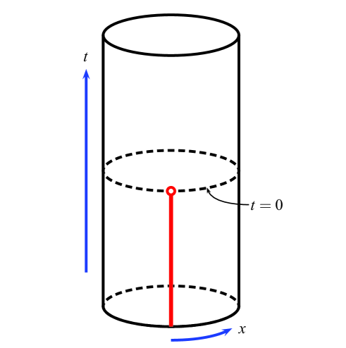
Figure 1: A graphical representation of the spacetime $\mathbb{R}\times S^{1}$, with time increasing in the vertical direction. The dashed circle midway up the cylinder shows the $t=0$ Cauchy surface. The red line shows the location of the delta-function potential that is turned off at $t=0$.

The Mamev-Trunov-type potential breaks the spacetime into two regions: a static IN region for $t<0$ where the scalar field is coupled to a non-zero delta-function potential, and a static OUT region for $t>0$ where the scalar field is free from the potential. A graphical representation of this spacetime with the potential is presented in Fig. 1.

In Sect. II, we determine the mode solutions to the Klein-Gordon-Fock wave equation for both regions. It is advantageous to separate the modes based on their spatial symmetry/antisymmetry properties about $x=0$. On the whole spacetime, both the IN and OUT regions, there exists a complete set of antisymmetric, orthonormal, positive-frequency, modes solutions of the form

$$\Phi^{\rm odd}(n,x,t)=(k_{n}L)^{-1/2}\,\sin(k_{n}x)\,e^{-ik_{n}t},$$ (33)

with $k_{n}=2\pi n/L$ and $n=1,2,3,\dots$. There are also negative-frequency antisymmetric mode solutions given by the complex conjugate. Because these modes vanish at the origin, they do not experience or interact with the potential.

There also exist symmetric, orthonormal, positive-frequency, mode solutions to the wave equation, which are sensitive to the potential, of the form

$$\Phi^{\rm even}(j,x,t)=\left\{\begin{array}[]{cc}\phi^{\rm even}(j,x,t)&\mbox{for }t\leq 0,\\[4.0pt] \phi^{\rm even}_{\rm OUT}(j,x,t)&\mbox{for }t\geq 0.\end{array}\right.$$ (34)

The IN portion of this mode solution is given by the expression

$$\phi^{\rm even}(j,x,t)=(\kappa_{j}L)^{-1/2}A_{j}\left[\cos(\kappa_{j}x)+\frac{\xi}{\kappa_{j}}\sin(\kappa_{j}|x|)\right]\,e^{-i\kappa_{j}t},$$ (35)

where $\kappa_{j}={2Z_{j}}/{L}$, $Z_{j}$ is the $j$-th positive root of the transcendental equation

$$Z=\frac{\xi L}{2}\cot(Z),$$ (36)

and $A_{j}$ is a normalization constant defined in Eq. (64) below. The IN portion of the modes solutions have a corner at the location of the delta-function potential, while the OUT portion have corners that propagate outward from the origin of the spacetime at the speed of light.

The OUT portion of the symmetric mode solution is given by a Fourier series, Eq. (94), in terms of the “standard” basis of symmetric modes for the potential-free Klein-Gordon equation, of which there are two kinds: a) an infinite family of time-oscillatory mode solutions, with the positive-frequency solutions given by

$$\psi^{\rm even}(n,x,t)=(k_{n}L)^{-1/2}\,\cos(k_{n}x)\,e^{-ik_{n}t},$$ (37)

where $k_{n}=2\pi n/L$, $n=1,2,3,\dots,$ and the negative-frequency solutions given by the complex conjugate, and b) two topological, zero-frequency, mode solutions given by

$$\psi^{\rm top.}(x,t)=\sqrt{\frac{\ell}{2L}}\left(1-i\frac{t}{\ell}\right)$$ (38)

and its complex conjugate. The topological modes exist because the spatial sections of the cylinder spacetime are compact. Furthermore, they are necessary to have a complete basis set to represent a solution to the Cauchy problem for all initial data. The antisymmetric, mode solutions, given by Eq. (33), do not appear in the Fourier representation for the OUT portion of the symmetric mode solutions on the whole spacetime.

To determine the Fourier coefficients for the OUT portion of the symmetric mode solution, we require, like Solommon, $C^{1}$ continuity (in time) of the complete mode solution across the $t=0$ Cauchy surface. Essentially, we are using the known behavior of the IN symmetric mode functions at time $t=0$ as the Cauchy data to determine a unique solution of the wave equation in the OUT region. The resulting Fourier series has non-zero Fourier coefficients, Eqs. (88) and (90), for both the topological modes and the positive and negative-frequency even mode solutions. Thus, the initially positive-frequency even mode solution on the IN region of the spacetime develops both positive and negative-frequency components at the moment that the potential turns off which persist through the OUT region.

In Sec. III, we second-quantize our system, following the standard canonical quantization scheme in literature (see, for example, Birrell and Davies Birrell and Davies (1982)). In this scheme, one promotes the real-valued classical field $\Phi$ to a self-adjoint operator $\bm{\Phi}$ on a Hilbert space of states. The typical Hilbert space is usually given by a standard Fock space. For a Bosonic field theory, the field operator and its conjugate momenta $\bm{\Pi}$ also satisfy a standard set of equal time commutation relations. This process works well for our spacetime because it has a convenient timelike Killing vector.

On the IN region of the spacetime, the Fock space associated with the field algebra has the usual form, and we define the IN vacuum state $|0_{L}\rangle$ to be the state destroyed by all of the annihilation operators of the field algebra, Eq. (103). The subscripted $L$ is included in the notation to remind us that this is the ground state on a spatially-closed spacetime of circumference $L$, and not the standard Minkowski-space vacuum state, which we will denote by $|0\rangle$. States with higher particle content can be constructed in the usual way by acting with the creation operators.

On the OUT region of the spacetime, there exists an unitarily equivalent field algebra based upon the “standard” mode solutions to the potential-free wave equation. So we also present the second-quantization of this equivalent system. However, we do make one modification to the standard quantization procedure; along with the time-oscillatory modes, we also second-quantize the topological modes using the method developed by Ford and Pathinayake Ford and Pathinayake (1989). At the classical level, the topological modes given by Eq. (38) have nonzero conjugate momenta, therefore they can be included in the classical symplectic form that gets lifted to the commutator relation of the field algebra. It is found that such a process produces an algebra with a non-trivial center Dappiaggi and Lang (2012).

Because the OUT region had two equivalent field algebras and Fock spaces, we determine the Bogolubov transformation between the elements of the algebras. Since the OUT portion of the symmetric mode solutions is already given by a Fourier series in terms of the “standard” modes, determining the explicit form of the Bogolubov coefficients is simply a task of identifying the correct Fourier coefficient.

Working in the Heisenberg picture, we then calculate the number of “standard” quanta created on the OUT region of the spacetime for the IN vacuum state $|0_{L}\rangle$. We find that (a) no quanta are created in the odd modes, (b) a finite, non-zero number of quanta are created in the topological modes, Eq. (121), (c) a finite, non-zero number of quanta are created in the time-oscillatory even modes, Eq. (122), and (d) the total number of quanta created is finite. All the quanta created in this model come into existence at the moment the potential is shut off, i.e., at $t=0$.

In Sec. IV, we determine the renormalized expectation value of the stress-tensor for the IN ground state $|0_{L}\rangle$ on both the IN and OUT regions of the spacetime. For the IN region of the spacetime we find

$$\langle 0_{L}|\bm{T}_{\mu\nu}|0_{L}\rangle_{Ren.}=\left(-\frac{\pi}{6L^{2}}+\frac{\mathcal{B}-\mathcal{C}}{L^{2}}\right)\delta_{\mu\nu},$$ (39)

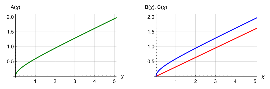
Figure 2: Plots of the coefficients $\mathcal{A}$ (green), $\mathcal{B}$ (blue), and $\mathcal{C}$ (red) as a function of the dimensionless variable $\chi$. The plots were generated in Mathematica by calculating the partial sum for the first $2^{15}$ terms of each infinite series. The plots seem to indicate that $\mathcal{A}=\mathcal{B}$. The analysis in Appendix C shows that $\mathcal{C}=\chi/\pi$, i.e., it is a straight line.

which holds everywhere except at the location of the delta-function potential. The $-\pi/6L^{2}$ part of this expression is the standard Casimir energy-density for the cylinder spacetime. The $(\mathcal{B}-\mathcal{C})/L^{2}$ is the correction to the ground state energy-density due to the presence of the potential. Here, both coefficients $\mathcal{B}$ and $\mathcal{C}$ are positive functions of $\chi\equiv\xi L/2$, given by infinite summations over the transcendental eigenvalues, Eqs. (142) and (156) respectively, and are plotted in Fig. 2. We explicitly prove that both are convergent, and we determine that the difference between them always satisfies

$$0\leq(\mathcal{B}-\mathcal{C})\leq\frac{\pi}{6}.$$ (40)

We also determine the renormalized expectation of the stress-tensor on the OUT region for the same state;

$$\langle 0_{L}|\bm{T}_{\mu\nu}|0_{L}\rangle_{Ren.} = \left\{-\frac{\pi}{6L^{2}}+\frac{\mathcal{B-C}}{L^{2}}+\frac{\mathcal{C}}{2L^{2}}\sum_{n=-\infty}^{\infty}\left[\delta\left(\frac{t+x}{L}-n\right)+\delta\left(\frac{t-x}{L}-n\right)\right]\right\}\delta_{\mu\nu}$$ (43)

$$+\frac{\mathcal{C}}{2L^{2}}\sum_{n=-\infty}^{\infty}\left[\delta\left(\frac{t+x}{L}-n\right)-\delta\left(\frac{t-x}{L}-n\right)\right]\left(\begin{array}[]{cc}0&1\\ 1&0\end{array}\right),$$

which holds for all spacetime locations to the future of the $t=0$ Cauchy surface. It is covariantly conserved, i.e., $\nabla^{\mu}\langle 0_{L}|\bm{T}_{\mu\nu}|0_{L}\rangle_{Ren.}=0$, and we find the standard Casimir energy-density for the cylinder spacetime followed by a correction to the ground state energy-density given by the $(\mathcal{B}-\mathcal{C})/L^{2}$ term. The remaining terms in the above expression are the contributions to the stress-tensor due to the quanta excited (i.e. particle creation) from the shutting off of the potential. The remarkably simple expression of two classical, point-like particles moving outward from the origin to the left and right with equal amplitude $\mathcal{C}/2$ is the result of a very detailed analysis of the properties of the Bogolubov coefficients and identities, and their application to the very complicated expression for the “moving” parts of the stress-tensor given by the Fourier series in Eq. (144).

In Sec. V, we evaluate the energy conditions from general relativity on the OUT region of the spacetime, using the expression above for the renormalized stress-tensor. For a timelike geodesic worldline, the renormalized expectation value of the energy-density is given by Eq. (201), and for a null geodesic worldline by Eq. (206). We find that the null energy condition (NEC), weak energy condition (WEC), the strong energy condition (SEC), and the dominant energy condition (DEC) all fail on some region of the space-time for the OUT-region stress-tensor because the difference $\mathcal{B}-\mathcal{C}\leq\pi/6$, and is therefore insufficiently large to overcome the usual $-\pi/6L^{2}$ term of the Casimir energy. We then calculate the total energy in a constant-time Cauchy surface on the OUT region, finding

$$\mathcal{E}=-\frac{\pi}{6L}+\frac{\mathcal{B}}{L}.$$ (44)

We note that the total energy is a constant, independent of time, further indicating that the renormalized stress-tensor on the OUT region is conserved for all time $t>0$. Additionally, because of the dependance of $\mathcal{B}$ on the value of $\chi$, the total energy in the Cauchy surface is negative for values of $\chi\leq 0.82$, positive for values of $\chi\geq 0.83$, and it passes through zero somewhere in the range $0.82<\chi<0.83$.

In the final part of Sec. V, we use our normal-ordered expectation value of the energy-density for the IN vacuum state on the OUT region in a QWEI for the two-dimensional cylinder spacetime without potential, given by

$$\int_{\mathbb{R}}d\tau\,\langle\omega|\bm{\rho}|\omega\rangle_{\rm Ren.}(\tau)\left[g(\tau)\right]^{2} \geq \frac{1+v^{2}}{1-v^{2}}\left(-\frac{\pi}{6L^{2}}\right)\int_{\mathbb{R}}d\tau\,\left[g(\tau)\right]^{2}-\frac{1}{2L}\sum_{n=1}^{\infty}k_{n}\left[\frac{1+v}{1-v}\int_{0}^{\infty}\frac{d\alpha}{\pi}\left|\hat{g}\left(\alpha+k_{n}\sqrt{\frac{1+v}{1-v}}\right)\right|^{2}\right.$$ (45)

$$\left.+\frac{1-v}{1+v}\int_{0}^{\infty}\frac{d\alpha}{\pi}\left|\hat{g}\left(\alpha+k_{n}\sqrt{\frac{1-v}{1+v}}\right)\right|^{2}\right],$$

where $|\omega\rangle$ is any Hadamard state on the cylinder spacetime, and $g(\tau)$ is a smooth, real-valued, compactly-supported test function on real line. The derivation of this QWEI, with the inclusion of the topological modes, is contained in Appendix E. We can use this inequality on the OUT region of our spacetime if we restrict the set of test functions to only those which have compact support to the future of the $t=0$ Cauchy surface.

Evaluating the left-hand side of the inequality for the state $|0_{L}\rangle$ yields

$$L.H.S = \int d\tau\,\langle 0_{L}|:\bm{\rho}:_{\tilde{0}_{L}}|0_{L}\rangle[g(\tau)]^{2}$$ (46)

$$= \frac{1+v^{2}}{1-v^{2}}\left(-\frac{\pi}{6L^{2}}\right)\int d\tau\,[g(\tau)]^{2}+\frac{1+v^{2}}{1-v^{2}}\left(\frac{\mathcal{B-C}}{L^{2}}\right)\int d\tau[g(\tau)]^{2}$$

$$+\frac{\mathcal{C}}{2L^{2}}\sum_{n=-\infty}^{\infty}\left[\frac{1+v}{1-v}\int d\tau[g(\tau)]^{2}\delta\left(\frac{t_{0}+x_{0}+(1+v)\gamma\tau}{L}-n\right)\right.$$

$$\left.+\frac{1-v}{1+v}\int d\tau[g(\tau)]^{2}\delta\left(\frac{t_{0}-x_{0}+(1-v)\gamma\tau}{L}-n\right)\right].$$

Notice that only the first of the four terms in the result for the left-hand side is negative, and that it is identical to the first term on the right-hand side of the QWEI. The remaining terms on the right-hand side are negative. Thus, the QWEI is satisfied by the stress-energy tensor of the IN vacuum state on the OUT region of the spacetime for all allowed test functions $g(t)$ with support to the future of the $t=0$ Cauchy surface, and for all values of $\xi$.

The main body of the paper concludes with some comments and conjectures in Sec. VI. In addition to the main body, there are five appendices containing technical information necessary for the paper to be complete, and to which we refer throughout the document. The appendices include: a proof of the equivalence of the IN and OUT region mode functions on a bow-tie shaped domain surrounding the $t=0$ Cauchy surface; the construction of the advanced-minus-retarded Green’s function on the cylinder spacetime when topological modes are included; the convergence and properties of certain summations over the eigenvalues of the transcendental equation; notes on an alternative way to determine the IN vacuum stress-tensor on the IN region and why it fails; and finally the derivation of the QWEI on the cylinder spacetime.

I.4 Mathematical Notation

We use units in which $\hbar$, $c$ and $G$ are set to unity throughout the paper. The complex conjugate of a complex number $z\in\mathbb{C}$ is denoted by $\overline{z}$, and similarly for functions. For complex-valued functions $u(x)$ and $v(x)$, we use the standard L² inner-product,

$$(u,v)_{L^{2}}\equiv\int_{S^{1}}u(x)\overline{v(x)}\,dx.$$ (47)

The normalization for mode solutions of the wave equation is chosen such that the modes are pseudo-orthonormal with respect to the standard bilinear product used in QFT Birrell and Davies (1982),

$$\left(\phi_{1},\phi_{2}\right)_{\rm QFT}\equiv-i\int_{-L/2}^{L/2}\left[\phi_{1}(x,t)\left(\partial_{t}\overline{\phi_{2}}(x,t)\right)-\left(\partial_{t}\phi_{1}(x,t)\right)\overline{\phi_{2}}(x,t)\right]dx.$$ (48)

Operators will be typeset in bold face to distinguish then from variables and functions. The Hermitian conjugate of an operator $\bm{a}$ will be denoted by $\bm{a}^{\dagger}$.

We define the Fourier transform on a Schwartz class function $f\in\mathcal{S}(\mathbb{R})$, the space of smooth functions that decay at infinity, as

$$\hat{f}(\alpha)=\int_{-\infty}^{\infty}f(x)\,e^{i\alpha x}dx.$$ (49)

Since the Fourier transform is an automorphism on Schwartz class functions, we have that the inverse Fourier transform is

$$f(x)=\frac{1}{2\pi}\int_{-\infty}^{\infty}\hat{f}(\alpha)\,e^{-i\alpha x}d\alpha.$$ (50)

For this choice of definition of the Fourier transform, the convolution theorem states

$$\int_{-\infty}^{\infty}f(x)g(y-x)dx=\frac{1}{2\pi}\int_{-\infty}^{\infty}\hat{f}(\alpha)\hat{g}(\alpha)\,e^{-i\alpha y}d\alpha,$$ (51)

which has as a corollary Parseval’s theorem,

$$\int_{-\infty}^{\infty}|f(x)|^{2}dx=\frac{1}{2\pi}\int_{-\infty}^{\infty}|\hat{f}(\alpha)|^{2}d\alpha.$$ (52)

II The Classical Formalism

Let $\mathcal{M}$ be an $n$-dimensional, globally hyperbolic, Lorentzian spacetime with smooth metric $\bm{g}$ of signature $(+,-,\dots,-)$. On this spacetime we have a real-valued scalar field $\phi:\mathcal{M}\rightarrow\mathbb{R}$, which interacts with a scalar potential $V(x)$. This situation is described by the action

$$S_{\rm matter}(\phi,g^{\mu\nu})=\frac{1}{2}\int\left[g^{\mu\nu}\left(\partial_{\mu}\phi\right)\left(\partial_{\nu}\phi\right)-V(x)\phi^{2}\right]\sqrt{-g}\,d^{n}x,$$ (53)

where $g_{\mu\nu}$ is the spacetime metric, $g=\det{g_{\mu\nu}}$, $g^{\mu\nu}$ is the inverse of the metric, and $\partial_{\mu}$ is the partial derivative. Variation of the action with respect to the scalar field yields the standard Klein-Gordon-Fock wave equation

$$\frac{1}{\sqrt{-g}}\partial_{\mu}\sqrt{-g}g^{\mu\nu}\partial_{\nu}\phi+V\phi=0,$$ (54)

or, more succinctly, $\Box\phi+V\phi=0$. Similarly, the stress-tensor is found by varying the action with respect to the inverse-metric. When considered with the gravitational action Wald (1984), the stress-tensor for minimal coupling has the form

$$T_{\mu\nu}=(\partial_{\mu}\phi)(\partial_{\nu}\phi)-\frac{1}{2}g_{\mu\nu}\left[g^{\alpha\beta}(\partial_{\alpha}\phi)(\partial_{\beta}\phi)-V\phi^{2}\right].$$ (55)

We now make a two choices so that the mathematics which follows is more tractable. First, we choose to work on the the standard two-dimensional cylinder spacetime $\mathbb{R}\times S^{1}$. This is done for two reasons: a) the spactime is boundaryless so there are no boundary conditions to consider, and b) the spectrum of the Laplace operator on $S^{1}$, with and without the potential, is discreet. We use the standard Minkowski space $(t,x)$ coordinates with the identification of points such that $(t,x)=(t,x+L)$. Here, $L$ is the circumference of the spatial sections of the universe. Secondly, on this spacetime we have a scalar, Mamev-Trunov-type potential Mamev and Trunov (1982) given by Eq. (32).

The classical mode functions to the wave equation can be solved for independently in both regions. To determine mode functions on the whole spacetime, we take each mode function from the IN region and require that the function and its first derivative match across the $t=0$ Cauchy surface to a general Fourier decomposition of the wave function in the OUT region, i.e. we require $C^{1}$ continuity in $t$ of the wave functions. This matching is used to determine the Fourier coefficients for the OUT solution of the wave solution. We now present the details of this process.

II.1 Mode Solutions on the IN Region, $t<0$

For our spacetime, and upon substitution of the potential, the wave equation for the IN region is

$$\partial_{t}^{2}\phi-\partial_{x}^{2}\phi+2\xi\,\delta(x)\phi=0.$$ (56)

Using the standard techniques for separation of variables, we assume a solution of the form $\phi(x,t)=u(x)T(t)$, such that the time dependence solves

$$T_{tt}(t)+\lambda T(t)=0,$$ (57)

while the space dependence leads to the Schrödinger-like equation

$$-u_{xx}(x)+2\xi\,\delta(x)u(x)=\lambda u(x).$$ (58)

Here, $\lambda$ is the separation constant, playing a role akin to the energy in ordinary quantum mechanics. The operator

$$\bm{O}=-\frac{d^{2}}{dx^{2}}+2\xi\,\delta(x)$$ (59)

is Hermitian, i.e., $(u,\bm{O}v)_{L^{2}}=(\bm{O}u,v)_{L^{2}}$, with respect to the standard $L^{2}$ inner product on $S^{1}$.

The spatial sections of the universe are compact, therefore the eigenvalues $\lambda$ are discrete. Furthermore, the eigenvalues are real-valued and greater than or equal to zero. A convenient $L^{2}$-orthonormalized basis of eigenfunction to Eq. (58) is given by (a) a family of antisymmetric eigenfunctions,

$$u^{\rm odd}(n,x)=\sqrt{\frac{2}{L}}\sin(k_{n}x),$$ (60)

where $k_{n}={2\pi n}/{L}$, $\lambda_{n}=(k_{n})^{2}$ and $n=1,2,3,\dots$, and (b) a family of symmetric eigenfunctions,

$$u^{\rm even}(j,x)=\sqrt{\frac{2}{L}}A_{j}\left[\cos(\kappa_{j}x)+\frac{\xi}{\kappa_{j}}\sin(\kappa_{j}|x|)\right],$$ (61)

where $\kappa_{j}={2Z_{j}}/{L}$, $\lambda_{j}=(\kappa_{j})^{2}$, and $Z_{j}$ is the $j$-th positive root of the transcendental equation

$$Z=\frac{\xi L}{2}\cot(Z).$$ (62)

For any value of $j$, the value of $Z_{j}$ lays in the interval between $(j-1)\pi$ and $(j-\frac{1}{2})\pi$. For $(j-1)>\xi L/2\pi$, the values of the $Z_{j}$’s approach the poles of the cotangent function from above. A fairly good approximation for $Z_{j}$ using the first two terms in the Taylor series of the cotangent function is

$$Z_{j} \approx (j-1)\pi+\frac{1}{2}\left(1+\frac{\chi}{3}\right)^{-1}\left[\sqrt{(j-1)^{2}\pi^{2}+4\chi\left(1+\frac{\chi}{3}\right)}-(j-1)\pi\right]$$ (63)

$$= (j-1)\pi+2\chi\left[(j-1)\pi+\sqrt{(j-1)^{2}\pi^{2}+4\chi\left(1+\frac{\chi}{3}\right)}\right]^{-1},$$

where $\chi=\xi L/2$. Strictly speaking, the exact value of $Z_{j}$ is always less that the value of the approximation above.

The normalization constant for the symmetric eigenfunctions is

$$A_{j}=\cos(Z_{j})\left[1+\frac{\sin(Z_{j})\cos(Z_{j})}{Z_{j}}\right]^{-1/2}.$$ (64)

There do not exist any eigenfunctions with eigenvalue $\lambda=0$.

From the above $L^{2}$-eigenfunctions, we can define positive-frequency mode solutions to the wave equation on the IN-region:

$$\phi^{\rm odd}(n,x,t)=(2k_{n})^{-1/2}u^{\rm odd}(n,x)\,e^{-ik_{n}t}$$ (65)

and

$$\phi^{\rm even}(j,x,t)=(2\kappa_{j})^{-1/2}u^{\rm even}(j,x)\,e^{-i\kappa_{j}t}.$$ (66)

The normalization for these mode solutions has been chosen such that the modes are orthonormal with respect to the standard bilinear product used in QFT, Eq. (48). Negative-frequency mode solutions are given by the complex conjugate of the above expressions.

II.2 Mode Solutions on the OUT Region, $t>0$

The OUT region is simply the spacetime $\mathbb{R}\times S^{1}$ with no potential, i.e., it is the standard cylinder spacetime. Assuming a solution of the form $\psi(x,t)=v(x)T(t)$, we find that the time dependence again solves Eq. (57), while the space dependence leads to

$$-v_{xx}(x)=\lambda v(x).$$ (67)

Here, $\lambda$ is again the separation constant. The eigenvalues and eigenfunctions to the spatial equation are well known; There are (a) antisymmetric eigenfunctions

$$v^{\rm odd}(n,x)=u^{\rm odd}(n,x),$$ (68)

(b) symmetric eigenfunctions

$$v^{\rm even}(n,x)=\sqrt{\frac{2}{L}}\cos(k_{n}x),$$ (69)

and (c) a zero-eigenvalue topological solution

$$v^{\rm top.}(x)=\frac{1}{\sqrt{L}}.$$ (70)

Both the symmetric and antisymmetric eigenfunctions have $k_{n}=2\pi n/L$ with $\lambda_{n}=(k_{n})^{2}$. A generic function on the circle can be represented as a Fourier series in this basis as

$$f(x)=c\,v^{\rm top.}(x)+\sum_{n=1}^{\infty}\left(a_{n}v^{\rm odd}(n,x)+b_{n}v^{\rm even}(n,x)\right),$$ (71)

where $c,\{a_{n}\}$, and $\{b_{n}\}$ are all Fourier coefficients. In particular, the Dirac $\delta$-function on $S^{1}$ has the representation

$$\delta(x-x^{\prime})=v^{\rm top.}(x)v^{\rm top.}(x^{\prime})+\sum_{n=1}^{\infty}\left(v^{\rm odd}(n,x)v^{\rm odd}(n,x^{\prime})+v^{\rm even}(n,x)v^{\rm even}(n,x^{\prime})\right).$$ (72)

The positive-frequency mode solutions to the wave equation on the OUT region for the antisymmetric and symmetric eigenfunctions are simply

$$\psi^{\rm odd}(n,x,t)=(2k_{n})^{-1/2}v^{\rm odd}(n,x)e^{-ik_{n}t}$$ (73)

and

$$\psi^{\rm even}(n,x,t)=(2k_{n})^{-1/2}v^{\rm even}(n,x)e^{-ik_{n}t},$$ (74)

respectively. The negative-frequency solutions are given by the complex conjugate of the above expressions. The topological eigenfunction leads to an often neglected solution of the wave equation,

$$\psi^{\rm top.}(x,t)=\sqrt{\frac{\ell}{2}}\,v^{\rm top.}(x)\left(1-i\frac{t}{\ell}\right)=\sqrt{\frac{\ell}{2L}}\left(1-i\frac{t}{\ell}\right),$$ (75)

where $\ell$ is an arbitrary constant that sets a length scale Ford and Pathinayake (1989). Unlike the time oscillatory solutions, the topological solution is not an eigenfunction of the energy operator $i\partial_{t}$. The complex conjugate of the topological solution is also a linearly independent solution of the wave equation. All three types of solutions are orthonormal with respect to the bilinear product Eq. (48), i.e., they satisfy

$$(\psi_{j},\psi_{j^{\prime}})_{\rm QFT}=\delta_{jj^{\prime}},\qquad(\overline{\psi_{j}},\overline{\psi_{j^{\prime}}})_{\rm QFT}=-\delta_{jj^{\prime}},\qquad\mbox{and}\qquad(\psi_{j},\overline{\psi_{j^{\prime}}})_{\rm QFT}=0.$$ (76)

where the labels $j$ and $j^{\prime}$ specify both the type of mode and the value of $n$.

A generic, complex-valued, classical solution to the wave equation in the OUT region is given by the Fourier series

$$\psi(x,t)=a\,\psi^{\rm top.}(x,t)+b\,\overline{\psi^{\rm top.}(x,t)}+\sum_{n=1}^{\infty}\left[a_{n}\psi^{\rm odd}(n,x,t)+b_{n}\overline{\psi^{\rm odd}(n,x,t)}+c_{n}\psi^{\rm even}(n,x,t)+d_{n}\overline{\psi^{\rm even}(n,x,t)}\right],$$ (77)

where $a$, $b$, $\{a_{n}\}$, $\{b_{n}\}$, $\{c_{n}\}$, and $\{d_{n}\}$ are complex-valued constants.

II.3 Mode Solutions on the Whole Spacetime

Next, we determine mode solutions on the whole of the spacetime for the time-dependent potential. Let $\phi(x,t)$ be any solution to the wave equation on the IN region. We know that a general solution in the OUT region is given by Eq. (77) above. At the $t=0$ Cauchy surface where the potential abruptly turns off, we require continuity of the wave function and its first time derivative, i.e.,

$$\phi(x,0)=\psi(x,0)\qquad\mbox{ and }\qquad\partial_{t}\phi(x,0)=\partial_{t}\psi(x,0).$$ (78)

Upon substitution, we find

$$\phi(x,0)=\sqrt{\frac{L}{2}}v^{\rm top}(x)(a+b)+\sum_{n=1}^{\infty}\frac{1}{\sqrt{2k_{n}}}\left[v^{\rm odd}(n,x)(a_{n}+b_{n})+v^{\rm even}(n,x)(c_{n}+d_{n})\right]$$ (79)

and

$$\partial_{t}\phi(x,0)=-\frac{i}{\sqrt{2L}}v^{\rm top}(x)(a-b)-i\sum_{n=1}^{\infty}\sqrt{\frac{k_{n}}{2}}\left[v^{\rm odd}(n,x)(a_{n}-b_{n})+v^{\rm even}(n,x)(c_{n}-d_{n})\right].$$ (80)

Next, we apply Fourier’s trick; put the above expressions into the first slot of the $L^{2}$ inner product with one of the OUT basis functions in the second slot. Permuting through all the basis functions results in

$$a = \frac{1}{\sqrt{2\ell}}\left(\phi(x,0)+i\ell\partial_{t}\phi(x,0),v^{\rm top.}(x)\right)_{L^{2}},$$ (81)

$$b = \frac{1}{\sqrt{2\ell}}\left(\phi(x,0)-i\ell\partial_{t}\phi(x,0),v^{\rm top.}(x)\right)_{L^{2}},$$ (82)

$$a_{n} = \sqrt{\frac{k_{n}}{2}}\left(\phi(x,0)-\frac{1}{ik_{n}}\partial_{t}\phi(x,0),v^{\rm odd}(n,x)\right)_{L^{2}},$$ (83)

$$b_{n} = \sqrt{\frac{k_{n}}{2}}\left(\phi(x,0)+\frac{1}{ik_{n}}\partial_{t}\phi(x,0),v^{\rm odd}(n,x)\right)_{L^{2}},$$ (84)

$$c_{n} = \sqrt{\frac{k_{n}}{2}}\left(\phi(x,0)-\frac{1}{ik_{n}}\partial_{t}\phi(x,0),v^{\rm even}(n,x)\right)_{L^{2}},$$ (85)

$$d_{n} = \sqrt{\frac{k_{n}}{2}}\left(\phi(x,0)+\frac{1}{ik_{n}}\partial_{t}\phi(x,0),v^{\rm even}(n,x)\right)_{L^{2}}.$$ (86)

We now explicitly determine these coefficients for the basis of IN mode solutions:

Odd Mode Solutions: If $\phi(x,t)=\phi^{\rm odd}(m,x,t)$ for $t\leq 0$, then $\phi(x,0)=(2k_{m})^{-1/2}v^{\rm odd}(m,x)$ and $\partial_{t}\phi(x,0)=-ik_{m}(2k_{m})^{-1/2}v^{\rm odd}(m,x)$. Upon substitution into the above expressions, we find $a=b=b_{n}=c_{n}=d_{n}=0$ for all $n$, and $a_{n}=\delta_{nm}$. So the antisymmetric, positive-frequency mode solutions to the wave equation on the whole spacetime is given by

$$\Phi^{\rm odd}(n,x,t)=(2k_{n})^{-1/2}\,u^{\rm odd}(n,x)\,e^{-ik_{n}t}\qquad\mbox{ with }\qquad k_{n}=\frac{2\pi n}{L}\mbox{ and }n=1,2,3,\dots.$$ (87)

This family of solutions, as well as its complex conjugate, are entirely ignorant to the presence of the potential.

Even Mode Solutions: If $\phi(x,t)=\phi^{\rm even}(j,x,t)$ for $t\leq 0$, then $\phi(x,0)=(2\kappa_{j})^{-1/2}u^{\rm even}(j,x)$ and $\partial_{t}\phi(x,0)=-i(\kappa_{j}/2)^{1/2}u^{\rm even}(j,x)$. Because both of the preceding expressions are even functions in the variable $x$, it is immediately obvious that $a_{n}=b_{n}=0$ for all $n$. Additionally,

$$a=\frac{1}{2\sqrt{\kappa_{j}\ell}}(1+\kappa_{j}\ell)Y_{j,0}\qquad\mbox{ and }\qquad b=\frac{1}{2\sqrt{\kappa_{j}\ell}}(1-\kappa_{j}\ell)Y_{j,0},$$ (88)

where the coefficient

$$Y_{j,0}=\left(u^{\rm even}(j,x),v^{\rm top.}(x)\right)_{L^{2}}=\frac{\xi LA_{j}}{\sqrt{2}Z_{j}^{2}}.$$ (89)

The remaining two sets of coefficients are found to be

$$c_{n}=\frac{1}{2}\sqrt{\frac{k_{n}}{\kappa_{j}}}\left(1+\frac{\kappa_{j}}{k_{n}}\right)Y_{j,n}\qquad\mbox{ and }\qquad d_{n}=\frac{1}{2}\sqrt{\frac{k_{n}}{\kappa_{j}}}\left(1-\frac{\kappa_{j}}{k_{n}}\right)Y_{j,n},$$ (90)

where

$$Y_{j,n}=\left(u^{\rm even}(j,x),v^{\rm even}(n,x)\right)_{L^{2}}=\frac{\xi LA_{j}}{Z_{j}^{2}-(\pi n)^{2}}.$$ (91)

Note, $Y_{j,0}$ is not the $n=0$ expression of $Y_{j,n}$; the two differ by a factor of $\sqrt{2}$. The $Y_{j,n}$’s turn out to be the Fourier coefficients for the Fourier series of $u^{\rm even}(j,x)$ when written in the OUT eigenfunctions, i.e.,

$$u^{\rm even}(j,x)=Y_{j,0}v^{\rm top.}(x)+\sum_{n=1}^{\infty}Y_{j,n}v^{\rm even}(n,x).$$ (92)

From the Bogolubov identities below, Eq. (125), one can demonstrate that the $Y_{j,n}$ coefficients satisfy

$$\sum_{j=1}^{\infty}Y_{j,m}Y_{j,n}=\delta_{mn},$$ (93)

where the allowed $m$ and $n$ also include zero.

Substituting the coefficients back into the Fourier decomposition of $\psi(x,t)$, we have that the time-evolution of an IN mode-solution into the OUT region is

$$\phi^{\rm even}_{\rm OUT}(j,x,t) = \sum_{n=0}^{\infty}\left[c_{n}\psi^{\rm even}(n,x,t)+d_{n}\overline{\psi^{\rm even}(n,x,t)}\right],$$ (94)

Here we are abusing our notation a bit with $\psi^{\rm even}(0,x,t)=\psi^{\rm top}(x,t)$, $c_{0}=a$ and $d_{0}=b$. We also wish to alert the reader that all of the Fourier coefficients given above are dependent upon the value of $j$ for the mode in question, although we have not explicitly written it that way. This notational deficiency will be rectified shortly when the Bogolubov coefficients are defined below.

On the whole of the spacetime, we have that the symmetric mode solutions to the wave equation are of the form

$$\Phi^{\rm even}(j,x,t)=\left\{\begin{array}[]{cc}\phi^{\rm even}(j,x,t)&\mbox{for }t\leq 0,\\[4.0pt] \phi^{\rm even}_{\rm OUT}(j,x,t)&\mbox{for }t\geq 0.\end{array}\right.$$ (95)

The symmetric modes start out as purely positive frequency, however, the shutting off of the potential at $t=0$ causes them to develop topological and negative frequency components.

There is one more important property of the symmetric mode solutions to the wave equation; we prove in Appendix A below that

$$\phi^{\rm even}(j,x,t)=\phi^{\rm even}_{\rm OUT}(j,x,t)$$ (96)

on the domain $\mathcal{D}\cup\{(0,0)\}$, where the open, bow-tie-shaped domain

$$\mathcal{D}\equiv\left\{(x,t)\in\left[-\frac{L}{2},\frac{L}{2}\right]\times\left[-\frac{L}{2},\frac{L}{2}\right]\big{|}-|x|<t<|x|\right\}.$$ (97)

In other words, we can extend the IN mode solutions to the future of $t=0$ Cauchy surface, and likewise extend the OUT mode solutions to the past of the same Cauchy surface. This is because of causality in the spacetime, i.e., the mode solutions don’t alter their behavior until information has had time to propagate outward from the location of the shutting off of the potential. So physically and mathematically we actually have

$$\Phi^{\rm even}(j,x,t)=\left\{\begin{array}[]{cl}\phi^{\rm even}(j,x,t)&\mbox{for }t<|x|,\\[4.0pt] \phi^{\rm even}(j,0,0)=\phi^{\rm even}_{\rm OUT}(j,0,0)&\mbox{for }t=x=0,\\[4.0pt] \phi^{\rm even}_{\rm OUT}(j,x,t)&\mbox{for }t>-|x|.\end{array}\right.$$ (98)

A generic complex-valued classical solution to the wave equation on the whole spacetime is given by the Fourier series

$$\Phi(x,t)=\sum_{n=1}^{\infty}\left[\alpha_{n}\Phi^{\rm odd}(n,x,t)+\alpha_{n}^{*}\overline{\Phi^{\rm odd}(n,x,t)}\right]+\sum_{j=1}^{\infty}\left[\beta_{j}\Phi^{\rm even}(j,x,t)+\beta_{j}^{*}\overline{\Phi^{\rm even}(j,x,t)}\right]$$ (99)

where $\{\alpha_{n}\}$, $\{\alpha^{*}_{n}\}$, $\{\beta_{n}\}$, $\{\beta^{*}_{n}\}$ are complex-valued constants.

We have seen that the odd mode solutions are unaffected by the delta-function potential, and therefore remain monochromatic with the same positive frequency. On the other hand, the even mode solutions change behavior when the delta-function is turned off, so even classically, the initially monochromatic positive frequency solution develops polychromatic positive and negative frequency components in the OUT region. Also notice that the mode solutions contain a contribution from the topological mode. In the quantum treatment of this problem, we will see that both of these give rise to particle creation at the moment the potential turns off.

III Canonical Quantization

To second-quantize our system, we will follow the standard canonical quantization scheme in literature (see, for example, Birrell and Davies Birrell and Davies (1982)). In this scheme, one lifts the real-valued classical field $\Phi$ to a self-adjoint operator $\bm{\Phi}$ on a Hilbert space of states. The typical Hilbert space is usually given by a Fock representation. For a Bosonic field theory, the field operator and its conjugate momenta $\bm{\Pi}$ must also satisfy a standard set of equal time commutation relations. This process works well for our spacetime because it has a convenient timelike Killing vector.

III.1 Quantization of the Field Operator on $\mathbb{R}\times S^{1}$ with Potential

For real-valued fields based on Eq. (99), we must require $\alpha_{n}^{*}=\overline{\alpha_{n}}$ and $\beta_{n}^{*}=\overline{\beta_{n}}$. Next, we promote the Fourier coefficients to operators on a Hilbert space, i.e., $a_{n}\mapsto\bm{a}_{n}$ and $b_{j}\mapsto\bm{b}_{j}$, to form a self-adjoint field operator

$$\bm{\Phi}(x,t)=\sum_{n=1}^{\infty}\left[\bm{a}_{n}\Phi^{\rm odd}(n,x,t)+\bm{a}_{n}^{\dagger}\overline{\Phi^{\rm odd}(n,x,t)}\right]+\sum_{j=1}^{\infty}\left[\bm{b}_{j}\Phi^{\rm even}(j,x,t)+\bm{b}_{j}^{\dagger}\overline{\Phi^{\rm even}(j,x,t)}\right].$$ (100)

Here, $\dagger$ specifies the Hermitian conjugate and. The field operator must also satisfy the equal time commutation relations

$$\left[\bm{\Phi}(x,t),\bm{\Phi}(x^{\prime},t)\right]=0=\left[\bm{\Pi}(x,t),\bm{\Pi}(x^{\prime},t)\right]\qquad\mbox{ and }\qquad\left[\bm{\Phi}(x,t),\bm{\Pi}(x^{\prime},t)\right]=i\delta(x-x^{\prime})\mathbb{I},$$ (101)

where $\bm{\Pi}(x,t)\equiv\partial_{t}\bm{\Phi}(x,t)$ and $\mathbb{I}$ is the identity operator. These commutation relationships hold if the operators $\bm{a}_{n}$ and $\bm{b}_{j}$ are required to satisfy

$$[\bm{a}_{n},\bm{a}_{m}^{\dagger}]=\delta_{nm}\mathbb{I}\qquad\mbox{ and }\qquad[\bm{b}_{j},\bm{b}_{j^{\prime}}^{\dagger}]=\delta_{jj^{\prime}}\mathbb{I},$$ (102)

with all other commutators vanishing.

The vacuum state for the IN region, which we will denote by $|0_{L}\rangle$, satisfies

$$\bm{a}_{n}|0_{L}\rangle=0=\bm{b}_{j}|0_{L}\rangle$$ (103)

for all $n$ and $j$. One-particle states are created by acting on the vacuum state with the creation operators $\bm{a}_{n}^{\dagger}$ and $\bm{b}_{j}^{\dagger}$, i.e.,

$$|1_{L,n}\rangle=\bm{a}_{n}^{\dagger}|0_{L}\rangle\qquad\mbox{ and }\qquad|1_{L,j}\rangle=\bm{b}_{j}^{\dagger}|0_{L}\rangle.$$ (104)

One can construct higher number particle states by repeated action of the creation operators.

The positive-frequency Wightman’s function is the vacuum expectation value of the point-split field-squared operator,

$$G^{+}(x,t;x^{\prime},t^{\prime}) = \langle 0_{L}|\bm{\Phi}(x,t)\bm{\Phi}(x^{\prime},t^{\prime})|0_{L}\rangle$$ (105)

$$= \frac{1}{2}\sum_{n=1}^{\infty}k_{n}^{-1}u^{\rm odd}(n,x)\overline{u^{\rm odd}(n,x^{\prime})}e^{-ik_{n}(t-t^{\prime})}+\sum_{j=1}^{\infty}\Phi^{\rm even}(j,x,t)\overline{\Phi^{\rm even}(j,x^{\prime},t^{\prime})}$$

The form of the Wightman’s function varies depending on the time coordinates, i.e., if $t$ and $t^{\prime}$ are on the IN or OUT regions of the spacetime. In particular, for the IN region, the Wightman’s function has the form

$$G^{+}_{\rm IN}(x,t;x^{\prime},t^{\prime})=\frac{1}{2}\left[\sum_{n=1}^{\infty}\frac{1}{k_{n}}u^{\rm odd}(n,x)\overline{u^{\rm odd}(n,x^{\prime})}e^{-ik_{n}(t-t^{\prime})}+\sum_{j=1}^{\infty}\frac{1}{\kappa_{j}}u^{\rm even}(j,x)\overline{u^{\rm even}(j,x^{\prime})}e^{-i\kappa_{j}(t-t^{\prime})}\right].$$ (106)

The form for the Wightman function for the OUT region will be given after the definition of the Bogolobuv coefficients below. (See Eq. (127) for the explicit form.)

III.2 Unitarily Equivalent Representation of the Field Operator for the OUT Region

For the OUT region of the spacetime, we have seen above that there is a second complete set of orthormal modes solutions to the wave equation given in terms of the odd modes Eq. (73), the even modes Eq. (74), and the topological modes Eq. (75). As in the preceding subsection, we can promote Eq. (77) to a real-valued, self-adjoint field operator, with

$$\bm{\psi}(x,t)=\widetilde{\bm{a}}\,\psi^{\rm top.}(x,t)+\widetilde{\bm{a}}^{\dagger}\,\overline{\psi^{\rm top.}(x,t)}+\sum_{n=1}^{\infty}\left[\widetilde{\bm{a}}_{n}\,\psi^{\rm odd}(n,x,t)+\widetilde{\bm{a}}_{n}^{\dagger}\,\overline{\psi^{\rm odd}(n,x,t)}+\widetilde{\bm{b}}_{n}\,\psi^{\rm even}(n,x,t)+\widetilde{\bm{b}}_{n}^{\dagger}\,\overline{\psi^{\rm even}(n,x,t)}\right],$$ (107)

where we assume the commutation relations Ford and Pathinayake (1989)

$$[\widetilde{\bm{a}},\widetilde{\bm{a}}^{\dagger}]=\mathbb{I}\qquad\mbox{ and }\qquad[\widetilde{\bm{a}}_{n},\widetilde{\bm{a}}_{m}^{\dagger}]=\delta_{nm}\mathbb{I}=[\widetilde{\bm{b}}_{n},\widetilde{\bm{b}}_{m}^{\dagger}],$$ (108)

with all other commutators vanishing.

It is straightforward to show that this yields the correct equal-time commutation relations for the field operator and its conjugate momenta $\bm{\pi}(x,t)\equiv\partial_{t}\bm{\psi}(x,t)$. Substituting, we have

$$\left[\bm{\psi}(x,t),\bm{\pi}(x^{\prime},t)\right] = i\left[v^{\rm top.}(x)v^{\rm top.}(x^{\prime})+\sum_{n=1}^{\infty}\left(v^{\rm odd}(x)v^{\rm odd}(x^{\prime})+v^{\rm even}(x)v^{\rm even}(x^{\prime})\right)\right].$$ (109)

By Eq. (72) above, this expression reduces to the standard $\left[\bm{\psi}(x,t),\bm{\pi}(x^{\prime},t)\right]=i\delta(x-x^{\prime})\mathbb{I}.$ It is also straightforward to demonstrate that

$$\left[\bm{\psi}(x,t),\bm{\psi}(x^{\prime},t)\right]=\left[\bm{\pi}(x,t),\bm{\pi}(x^{\prime},t)\right]=0\qquad\mbox{ and }\qquad\left[\bm{\psi}(x,t),\bm{\psi}(x^{\prime},t^{\prime})\right]=iE(x,t;x^{\prime},t^{\prime})\,\mathbb{I},$$ (110)

where $E(x,t;x^{\prime},t^{\prime})$ is the advanced-minus-retarded two point function on $\mathbb{R}\times S^{1}$ constructed in Appendix B.

The Hilbert space on which these operators act is given by the conventional Fock space used in QFT; the ground state with respect to this field operator is $|\tilde{0}_{L}\rangle$, such that

$$\widetilde{\bm{a}}|\tilde{0}_{L}\rangle=0\qquad\mbox{ and }\qquad\widetilde{\bm{a}}_{n}|\tilde{0}_{L}\rangle=0=\widetilde{\bm{b}}_{n}|\tilde{0}_{L}\rangle\qquad\forall\,n.$$ (111)

The positive-frequency Wightman function is quickly found to be

$$\tilde{G}^{+}(x,t;x^{\prime},t^{\prime}) = \langle\tilde{0}_{L}|\bm{\psi}(x,t)\bm{\psi}(x^{\prime},t^{\prime})|\tilde{0}_{L}\rangle$$ (112)

$$= \frac{\ell}{2L}\left(1-i\frac{t}{\ell}\right)\left(1+i\frac{t^{\prime}}{\ell}\right)+\frac{1}{L}\sum_{n=1}^{\infty}k_{n}^{-1}\cos[k_{n}(x-x^{\prime})]e^{-ik_{n}(t-t^{\prime})}$$

$$= \frac{\ell}{2L}\left(1-i\frac{t}{\ell}\right)\left(1+i\frac{t^{\prime}}{\ell}\right)-\frac{1}{4\pi}\ln\left\{\left[1-e^{-i2\pi(\Delta t-\Delta x)/L}\right]\left[1-e^{-i2\pi(\Delta t+\Delta x)/L}\right]\right\}$$ (113)

where $\Delta x=x-x^{\prime}$ and $\Delta t=t-t^{\prime}$.

One final note before we leave this section. With the specification and properties of the Bogolubov coefficients below, it is a straightforward exercise to check that for the OUT region $\langle\widetilde{0}_{L}|\bm{\Phi}(x,t)\bm{\Phi}(x^{\prime},t^{\prime})|\widetilde{0}_{L}\rangle=\widetilde{G}^{+}(x,t;x^{\prime},t^{\prime})$, as expected.

III.3 Bogolubov Transform and Particle Creation

For the OUT region, we have two representations for the field operator, one given in terms of the mode solutions on the whole spacetime, Eq.(100), and one given by the standard modes on $\mathbb{R}\times S^{1}$, Eq. (107). It is immediately obvious that the odd modes solutions are common to both representations, i.e., $\phi^{\rm odd}(n,x,t)=\psi^{\rm odd}(n,x,t)$, therefore $\widetilde{\bm{a}}_{n}=\bm{a}_{n}$ and $\widetilde{\bm{a}}_{n}^{\dagger}=\bm{a}_{n}^{\dagger}$, In keeping with the notation of Birrell and DaviesBirrell and Davies (1982), one can simply read the remaining Bogolubov coefficients from Eq. (94). We have

$$\overline{\alpha_{0j}} = a$$ (114)

$$\beta_{0j} = -b$$ (115)

$$\overline{\alpha_{nj}} = c_{n}$$ (116)

$$\beta_{nj} = -d_{n}$$ (117)

Therefore, on the OUT region, it is possible to express the $\mathbb{R}\times S^{1}$ annihilation and creation operators in terms of the annihilation and creation operators on the whole spacetime, i.e,

$$\widetilde{\bm{a}}=\sum_{j=1}^{\infty}(\overline{\alpha_{0j}}\,\bm{b}_{j}-\overline{\beta_{0j}}\,\bm{b}_{j}^{\dagger})\qquad\mbox{ and }\qquad\widetilde{\bm{b}}_{n}=\sum_{j=1}^{\infty}(\overline{\alpha_{nj}}\,\bm{b}_{j}-\overline{\beta_{nj}}\,\bm{b}_{j}^{\dagger}).$$ (118)

If the quantum state of the system is initially in the IN vacuum state, $|0_{L}\rangle$, then observers in the OUT region will observe the creation of field quanta with an expectation value per mode given by

$$\langle 0_{L}|\widetilde{\bm{N}}_{0}|0_{L}\rangle=\langle 0_{L}|\widetilde{\bm{a}}^{\dagger}\widetilde{\bm{a}}|0_{L}\rangle=\sum_{j=1}^{\infty}\left|\beta_{0j}\right|^{2}$$ (119)

for the topological modes, and

$$\langle 0_{L}|\widetilde{\bm{N}}_{n}|0_{L}\rangle=\langle 0_{L}|\widetilde{\bm{b}}_{n}^{\dagger}\widetilde{\bm{b}}_{n}|0_{L}\rangle=\sum_{j=1}^{\infty}\left|\beta_{nj}\right|^{2}$$ (120)

for the even modes. No quanta are created in the odd modes. By definition, the number of quanta created is a strictly positive quantity. Substituting the expressions for the Bogolubov coefficients and using Eq. (93), we find

$$\langle 0_{L}|\widetilde{\bm{N}}_{0}|0_{L}\rangle = -\frac{1}{2}+\frac{1}{4}\sum_{j=1}^{\infty}\left(\frac{1}{\kappa_{j}\ell}+\kappa_{j}\ell\right)Y_{j,0}^{2}$$ (121)

$$= -\frac{1}{2}+\left(\frac{\xi L}{2}\right)^{2}\left(\frac{\ell}{L}\right)\sum_{j=1}^{\infty}\left[Z_{j}^{2}+\left(\frac{L}{2\ell}\right)^{2}\right]\frac{A_{j}^{2}}{Z_{j}^{5}}$$

$$= -\frac{1}{2}+\frac{\ell}{L}F_{3}(\chi)+\frac{1}{4}\frac{L}{\ell}F_{5}(\chi),$$

where the function $F_{n}(x)$ is defined in Appendix C, and

$$\langle 0_{L}|\widetilde{\bm{N}}_{n}|0_{L}\rangle=-\frac{1}{2}+\frac{1}{4}\sum_{j=1}^{\infty}\left(\frac{k_{n}}{\kappa_{j}}+\frac{\kappa_{j}}{k_{n}}\right)Y_{j,n}^{2}=-\frac{1}{2}+\left(\frac{\xi L}{2}\right)^{2}\frac{1}{\pi n}\sum_{j=1}^{\infty}\frac{Z_{j}^{2}+(\pi n)^{2}}{\left[Z_{j}^{2}-(\pi n)^{2}\right]^{2}}\frac{A_{j}^{2}}{Z_{j}}.$$ (122)

Both $\langle 0_{L}|\widetilde{\bm{N}}_{0}|0_{L}\rangle$ and $\langle 0_{L}|\widetilde{\bm{N}}_{n}|0_{L}\rangle$ are absolutely convergent. Furthermore, the sum formed from the upper bound of these two sums is also absolutely convergent. Therefore, the total number of particles created at the shutting off of the potential is finite. Numerical values found using Mathematica for the first ten coefficients are presented in Table 1. The dominant pathway for particle creation is into the topological mode.

Table 1: Expectation value for the number of quanta excited per mode when the potential is turned off for various values of the coupling constant $\xi$. The values were generated using $L=1$ and summing the first 500 terms in the series using Mathematica. The $n=0$ values were determined with $\ell=L$.

	$\displaystyle\langle 0_{L}|\widetilde{\bm{N}}_{n}|0_{L}\rangle$
$n$	$\xi=1$	$\xi=5$	$\xi=10$	$\xi=100$
0	0.023987	0.255469	0.416834	1.082297
1	0.003875	0.024742	0.047086	0.198755
2	0.000665	0.005465	0.011781	0.070152
3	0.000231	0.002154	0.004975	0.036841
4	0.000108	0.001091	0.002639	0.022904
5	0.000059	0.000637	0.001594	0.015659
6	0.000036	0.000408	0.001048	0.011386
7	0.000024	0.000277	0.000731	0.008647
8	0.000017	0.000200	0.000533	0.006782
9	0.000012	0.000149	0.000402	0.005455
10	0.000009	0.000114	0.000312	0.004477

With the definition of the Bogolubov coefficients completed, we now give the expression for the Wightman’s function of the IN ground state on the OUT region of the spacetime. Making use of the series expansion of $\phi^{\rm even}_{\rm OUT}(j,x,t)$ in terms of the conventional modes on the OUT region, i.e.,

$$\phi^{\rm even}_{\rm OUT}(j,x,t)=\sum_{n=0}^{\infty}\left[\overline{\alpha_{nj}}\psi^{\rm even}(n,x,t)-\beta_{nj}\overline{\psi^{\rm even}(n,x,t)}\right],$$ (123)

we have

$$G^{+}_{\rm OUT}(x,t;x^{\prime},t^{\prime}) = \sum_{n=1}^{\infty}\phi^{\rm odd}(n,x,t)\overline{\phi^{\rm odd}(n,x^{\prime},t^{\prime})}$$ (124)

$$+\sum_{j=1}^{\infty}\sum_{n=0}^{\infty}\sum_{m=0}^{\infty}\left[\overline{\alpha_{nj}}\,\alpha_{mj}\,\psi^{\rm even}(n,x,t)\overline{\psi^{\rm even}(m,x^{\prime},t^{\prime})}-\overline{\alpha_{nj}}\,\overline{\beta_{mj}}\,\psi^{\rm even}(n,x,t)\psi^{\rm even}(m,x^{\prime},t^{\prime})\right.$$

$$\left.-\beta_{nj}\,\alpha_{mj}\,\overline{\psi^{\rm even}(n,x,t)}\overline{\psi^{\rm even}(m,x^{\prime},t^{\prime})}+\beta_{nj}\,\overline{\beta_{mj}}\,\overline{\psi^{\rm even}(n,x,t)}\psi^{\rm even}(m,x^{\prime},t^{\prime})\right].$$

Swapping the order of the $j$-summation with the $n$ and $m$ summations and using the properties of the Bogolubov coefficients,

$$\sum_{j=1}^{\infty}\left(\alpha_{mj}\,\overline{\alpha_{nj}}-\beta_{mj}\,\overline{\beta_{nj}}\right)=\delta_{nm}\qquad\mbox{ and }\qquad\sum_{j=1}^{\infty}\left(\alpha_{mj}\,\beta_{nj}-\beta_{mj}\,\alpha_{nj}\right)=0,$$ (125)

we can simplify the above expression to

$$G^{+}_{\rm OUT}(x,t;x^{\prime},t^{\prime}) = \sum_{n=1}^{\infty}\psi^{\rm odd}(n,x,t)\overline{\psi^{\rm odd}(n,x^{\prime},t^{\prime})}+\sum_{n=0}^{\infty}\psi^{\rm even}(n,x,t)\overline{\psi^{\rm even}(n,x^{\prime},t^{\prime})}$$ (126)

$$+2\operatorname{Re}\left\{\sum_{n=0}^{\infty}\sum_{m=0}^{\infty}\left[\left(\sum_{j=1}^{\infty}\overline{\beta_{nj}}\,\beta_{mj}\right)\psi^{\rm even}(n,x,t)\overline{\psi^{\rm even}(m,x^{\prime},t^{\prime})}\right.\right.$$

$$-\left.\left.\left(\sum_{j=1}^{\infty}\overline{\alpha_{nj}}\,\overline{\beta_{mj}}\right)\psi^{\rm even}(n,x,t)\psi^{\rm even}(m,x^{\prime},t^{\prime})\right]\right\}.$$

However, the first two summations are the definition of the positive-frequency Wightman function for the OUT ground state given by Eq. (113), thus

$$G^{+}_{\rm OUT}(x,t;x^{\prime},t^{\prime})-\widetilde{G}^{+}(x,t;x^{\prime},t^{\prime}) = 2\operatorname{Re}\left\{\sum_{n=0}^{\infty}\sum_{m=0}^{\infty}\left[\left(\sum_{j=1}^{\infty}\overline{\beta_{nj}}\,\beta_{mj}\right)\psi^{\rm even}(n,x,t)\overline{\psi^{\rm even}(m,x^{\prime},t^{\prime})}\right.\right.$$ (127)

$$-\left.\left.\left(\sum_{j=1}^{\infty}\overline{\alpha_{nj}}\,\overline{\beta_{mj}}\right)\psi^{\rm even}(n,x,t)\psi^{\rm even}(m,x^{\prime},t^{\prime})\right]\right\}.$$

We will determine the renormalized expectation value of the stress-energy tensor in the OUT region using this expression in the next section. Two final notes: first, both of the summations over $j$ in the above expression are absolutely convergent, and second, on the domain $\mathcal{D}\cup\{(0,0)\}$ the IN and OUT Wightman functions can be used interchangeably, i.e.,

$$G^{+}_{\rm OUT}(x,t;x^{\prime},t^{\prime})=G^{+}_{\rm IN}(x,t;x^{\prime},t^{\prime}).$$ (128)

This second property follows from the mode solutions being equal on the domain $\mathcal{D}\cup\{(0,0)\}$.

IV Stress-Energy Tensor

With the second quantization of the field now completed, we address the expectation value of the stress-tensor. The classical stress-tensor, Eq. (55), is promoted to the self-adjoint operator

$$\bm{T}_{\mu\nu}=\frac{1}{2}\left\{(\partial_{\mu}\bm{\Phi})(\partial_{\nu}\bm{\Phi})+(\partial_{\nu}\bm{\Phi})(\partial_{\mu}\bm{\Phi})-g_{\mu\nu}\left[g^{\alpha\beta}(\partial_{\alpha}\bm{\Phi})(\partial_{\beta}\bm{\Phi})-V\bm{\Phi}\bm{\Phi}\right]\right\}.$$ (129)

For any normalized state $|\chi_{L}\rangle$ in the Fock space, it is well know that the expectation value of the stress-tensor is divergent. For free fields in Minkowski spacetime, the divergences are removed by the normal ordering process, but in curved spacetimes and flat spacetimes of non-trivial topology, we are required to employ renormalization to obtain finite results. For a quantum field interacting with a potential, as here, further local renormalization counterterms are required which are dependent upon the potential. Mamev and Trunov discuss this in their paper and the references therein Mamev and Trunov (1982). Further work has been carried out by others, including Graham, Jaffe, and colleagues Graham et al. (2002); Graham and Olum (2003), working primarily in Minkowski spacetime.

This leaves us in an awkward position. Progress has been made on the two fronts, but we are unaware of both renormalizations being combined to fully treat the problem at hand. To do so here would be beyond the intent of this paper, so we follow the path of Mamev and Trunov who calculate the renormalized stress-tensor in regions of the spacetime where the potential is zero. For such localized potentials, the potential-dependent counterterms are not necessary outside of the support of the potential. This is the same path that Solomon takes, which gives rise to his notion of the kinetic-tensor. Thus, outside the support of the potential, we define

$$\langle\chi_{L}|\bm{T}_{\mu\nu}|\chi_{L}\rangle_{Ren.}\equiv\langle\chi_{L}|\bm{T}_{\mu\nu}|\chi_{L}\rangle-\langle 0|\bm{T}_{\mu\nu}|0\rangle$$ (130)

where $|0\rangle$ is the Minkowski vacuum state. The rigorous mathematical interpretation of this renormalization scheme is discussed by Kay Kay (1979).

The renormalized expectation value of the stress-tensor for the OUT vacuum state on the OUT region of the spacetime is identical to the determination of the Casimir effect in the standard $\mathbb{R}\times S^{1}$ spacetime that is found in literature. (For example, see Chap. 4 of Birrell and Davies, or Kay Kay (1979) and the references therein.) With the inclusion of the topological modes Ford and Pathinayake (1989), we have the simple expression

$$\langle\widetilde{0}_{L}|\bm{T}_{\mu\nu}|\widetilde{0}_{L}\rangle_{\rm Ren.}=\left(\frac{1}{4\ell L}-\frac{\pi}{6L^{2}}\right)\delta_{\mu\nu}.$$ (131)

Notice that the topological modes only add a positive-constant term to the renormalized stress-tensor. The additional term is dependent upon the arbitrary constant $\ell$.

For the calculation to follow below, we define normal ordering of the unrenormalized stress-tensor in any allowable state $|\chi_{L}\rangle$, with respect to any other allowable state $|\rho_{L}\rangle$, as

$$\langle\chi_{L}|:\bm{T}_{\mu\nu}:_{\rho_{L}}|\chi_{L}\rangle=\langle\chi_{L}|\bm{T}_{\mu\nu}|\chi_{L}\rangle-\langle\rho_{L}|\bm{T}_{\mu\nu}|\rho_{L}\rangle.$$ (132)

It is computationally useful to combine this with the renormalization scheme defined above, yielding

$$\langle\chi_{L}|\bm{T}_{\mu\nu}|\chi_{L}\rangle_{Ren.}=\langle\chi_{L}|:\bm{T}_{\mu\nu}:_{\rho_{L}}|\chi_{L}\rangle+\langle\rho_{L}|\bm{T}_{\mu\nu}|\rho_{L}\rangle_{Ren.}.$$ (133)

The remainder of this section is dedicated to determining expressions for each of the terms above when $|\chi_{L}\rangle=|0_{L}\rangle$ and $|\rho_{L}\rangle=|\tilde{0}_{L}\rangle$. Because the mode decompositon of the field changes at the $t=0$ Cauchy surface, the expression for the stress-tensor can be written as

$$\langle 0_{L}|\bm{T}_{\mu\nu}|0_{L}\rangle_{Ren.}=\left\{\begin{array}[]{ll}\langle 0_{L}|:\bm{T}_{\mu\nu}^{IN}:_{\widetilde{0}_{L}}|0_{L}\rangle+\langle\widetilde{0}_{L}|\bm{T}_{\mu\nu}|\widetilde{0}_{L}\rangle_{Ren.}&\mbox{for }t\leq 0,\\ \langle 0_{L}|:\bm{T}_{\mu\nu}^{OUT}:_{\widetilde{0}_{L}}|0_{L}\rangle+\langle\widetilde{0}_{L}|\bm{T}_{\mu\nu}|\widetilde{0}_{L}\rangle_{Ren.}&\mbox{for }t\geq 0.\end{array}\right.$$ (134)

IV.1 Renormalized Stress-Tensor for $|0_{L}\rangle$ on the OUT Region

For the OUT region, we can make progress toward an explicit expression if we first look at the ingoing ground state’s normal-ordered, point-split, field-squared operator,

$$\Delta G^{+}(x,t;x^{\prime},t^{\prime})=\langle 0_{L}|:\bm{\Phi}(x)\bm{\Phi}(x^{\prime}):_{\tilde{0}_{L}}|0_{L}\rangle=\langle 0_{L}|\bm{\Phi}(x)\bm{\Phi}(x^{\prime})|0_{L}\rangle-\langle\widetilde{0}_{L}|\bm{\Phi}(x)\bm{\Phi}(x^{\prime})|\widetilde{0}_{L}\rangle.$$ (135)

However, the right-hand side is the difference of the positive-frequency Wightman functions we determined above in Eq. (127). Recall, the $n=0$ topological mode is unique from the rest of the even modes, so we expand the products out;

$$\Delta G^{+}(x,t;x^{\prime},t^{\prime}) = 2\operatorname{Re}\left\{\left[\left(\sum_{j=1}^{\infty}|\beta_{0j}|^{2}\right)\psi^{\rm top.}(x,t)\overline{\psi^{\rm top.}(x^{\prime},t^{\prime})}-\left(\sum_{j=1}^{\infty}\overline{\alpha_{0j}}\,\overline{\beta_{0j}}\right)\psi^{\rm top.}(x,t)\psi^{\rm top.}(x^{\prime},t^{\prime})\right]\right.$$

$$+\sum_{m=1}^{\infty}\left[\left(\sum_{j=1}^{\infty}\overline{\beta_{0j}}\,\beta_{mj}\right)\psi^{\rm top.}(x,t)\overline{\psi^{\rm even}(m,x^{\prime},t^{\prime})}-\left(\sum_{j=1}^{\infty}\overline{\alpha_{0j}}\,\overline{\beta_{mj}}\right)\psi^{\rm top.}(x,t)\psi^{\rm even}(m,x^{\prime},t^{\prime})\right]$$

$$+\sum_{n=1}^{\infty}\left[\left(\sum_{j=1}^{\infty}\overline{\beta_{nj}}\,\beta_{0j}\right)\psi^{\rm even}(n,x,t)\overline{\psi^{\rm top.}(x^{\prime},t^{\prime})}-\left(\sum_{j=1}^{\infty}\overline{\alpha_{nj}}\,\overline{\beta_{0j}}\right)\psi^{\rm even}(n,x,t)\psi^{\rm top.}(x^{\prime},t^{\prime})\right]$$

$$+\left.\sum_{n=1}^{\infty}\sum_{m=1}^{\infty}\left[\left(\sum_{j=1}^{\infty}\overline{\beta_{nj}}\,\beta_{mj}\right)\psi^{\rm even}(n,x,t)\overline{\psi^{\rm even}(m,x^{\prime},t^{\prime})}\right.\right.$$

$$-\left.\left.\left(\sum_{j=1}^{\infty}\overline{\alpha_{nj}}\,\overline{\beta_{mj}}\right)\psi^{\rm even}(n,x,t)\psi^{\rm even}(m,x^{\prime},t^{\prime})\right]\right\}.$$

The expectation value of the normal-ordered energy-density for the IN ground state on the OUT region can be found from this expression by

$$\langle 0_{L}|:\bm{T}_{tt}:|0_{L}\rangle=\frac{1}{2}\lim_{(t^{\prime},x^{\prime})\rightarrow(t,x)}\left(\partial_{t}\partial_{t^{\prime}}+\partial_{x}\partial_{x^{\prime}}\right)\Delta G^{+}(x,t;x^{\prime},t^{\prime}).$$ (137)

Evaluating the derivatives and taking the limit as the spacetime points come together yields

$$\langle 0_{L}|:\bm{T}_{tt}:|0_{L}\rangle = \frac{1}{L}\left\{\sum_{n=1}^{\infty}k_{n}\sum_{j=1}^{\infty}|\beta_{nj}|^{2}+\frac{1}{2\ell}\sum_{j=1}^{\infty}\left[|\beta_{0j}|^{2}+\operatorname{Re}(\alpha_{0j}\beta_{0j})\right]\right\}+\operatorname{Re}\left[\rho(t-x)+\rho(t+x)\right]$$ (138)

$$= -\frac{1}{4\ell L}+\frac{\mathcal{B}}{L^{2}}+\operatorname{Re}\left[\rho(t-x)+\rho(t+x)\right],$$ (139)

where we have made use of the properties of the Bogolubov coefficients to simplify the summation,

$$\sum_{j=1}^{\infty}\left[|\beta_{0j}|^{2}+\operatorname{Re}(\alpha_{0j}\beta_{0j})\right]=-\frac{1}{2}+\frac{1}{2}\sum_{j=1}^{\infty}\left|\beta_{0j}+\overline{\alpha_{0j}}\right|^{2},$$ (140)

in order to define the positive constant

$$\mathcal{B}\equiv L\left(\sum_{n=1}^{\infty}k_{n}\sum_{j=1}^{\infty}|\beta_{nj}|^{2}+\frac{1}{4\ell}\sum_{j=1}^{\infty}|\beta_{0j}+\overline{\alpha_{0j}}|^{2}\right).$$ (141)

Upon substitution of the expressions for the Bogolubov coefficients, we find

$$\mathcal{B} = \frac{(\xi L)^{2}}{2}\sum_{n=1}^{\infty}\sum_{j=1}^{\infty}\frac{A_{j}^{2}}{Z_{j}(Z_{j}+\pi n)^{2}}+\frac{(\xi L)^{2}}{4}\sum_{j=1}^{\infty}\frac{A_{j}^{2}}{Z_{j}^{3}}$$ (142)

$$= \frac{(\xi L)^{2}}{2\pi^{2}}\sum_{j=1}^{\infty}\frac{A_{j}^{2}}{Z_{j}}\left[\psi^{(1)}\left(1+\frac{Z_{j}}{\pi}\right)+\frac{\pi^{2}}{2Z_{j}^{2}}\right],$$

where $\psi^{(1)}(x)$ is the polygamma function of order one (p. 260 of Abramowitz and Stegun (1965)). $\psi^{(1)}(x)$ is a positive, strictly decreasing function on the interval $x\in(0,\infty)$, with a pole of order-2 at $x=0$. (We have no interest in the polygamma function for values of $x<1$.) Also, $\psi^{(1)}(1)=\zeta(2)=\pi^{2}/6$, thus

$$\pi^{2}/6\geq\psi^{(1)}\left(1+\frac{z}{\pi}\right)>0$$ (143)

on the interval $z\in[0,\infty).$ One remarkable fact to note is that the constant $\mathcal{B}$ is independent of $\ell$.

The coordinate-dependent function $\rho$ is given by

$$\rho(z) \equiv \frac{1}{2L\sqrt{2\ell}}\sum_{n=1}^{\infty}k_{n}^{1/2}\left[e^{-ik_{n}z}\sum_{j=1}^{\infty}(\overline{\beta_{nj}}\beta_{0j}+\overline{\alpha_{nj}}\overline{\beta_{0j}}+\overline{\alpha_{0j}}\overline{\beta_{nj}})+e^{ik_{n}z}\sum_{j=1}^{\infty}\overline{\beta_{0j}}\beta_{nj}\right]$$ (144)

$$+\frac{1}{2L}\sum_{n=1}^{\infty}\sum_{m=1}^{\infty}(k_{n}k_{m})^{1/2}\left[(1-\delta_{nm})e^{-i(k_{n}-k_{m})z}\sum_{j=1}^{\infty}\overline{\beta_{nj}}\beta_{mj}+e^{-i(k_{n}+k_{m})z}\sum_{j=1}^{\infty}\overline{\alpha_{nj}}\overline{\beta_{mj}}\right].$$

For this particular case, the Bogolubov coefficients are all real valued and we find

$$\operatorname{Re}\rho(z) = \frac{1}{2L\sqrt{2\ell}}\sum_{n=1}^{\infty}k_{n}^{1/2}\cos(k_{n}z)\sum_{j=1}^{\infty}(2\beta_{nj}\beta_{0j}+\alpha_{nj}\beta_{0j}+\alpha_{0j}\beta_{nj})$$ (145)

$$+\frac{1}{2L}\sum_{n=1}^{\infty}\sum_{m=1}^{\infty}(k_{n}k_{m})^{1/2}\left\{(1-\delta_{nm})\cos\left[(k_{n}-k_{m})z\right]\sum_{j=1}^{\infty}\beta_{nj}\beta_{mj}+\cos\left[(k_{n}+k_{m})z\right]\sum_{j=1}^{\infty}\alpha_{nj}\beta_{mj}\right\}.$$

The double summations of $n$ and $m$ over the above range can be reorganized to simplify our expression.

Upon substitution for the Bogolubov coefficients, we have

$$\operatorname{Re}\rho(z) = \frac{1}{2L}\left\{\sum_{n=1}^{\infty}\cos(k_{n}z)\left[\frac{1}{2\sqrt{2}}\sum_{j=1}^{\infty}\left(2\kappa_{j}-k_{n}-\frac{1}{\ell}\right)Y_{j,0}Y_{j,n}\right]\right.$$ (146)

$$+\sum_{n=1}^{\infty}\cos(k_{n}z)\left[\frac{1}{2}\sum_{m=1}^{\infty}\sum_{j=1}^{\infty}\frac{1}{\kappa_{j}}(\kappa_{j}-k_{m})(\kappa_{j}-k_{n+m})Y_{j,m}Y_{j,n+m}\right]$$

$$+\left.\sum_{n=2}^{\infty}\cos(k_{n}z)\left[\frac{1}{4}\sum_{m=1}^{n-1}\sum_{j=1}^{\infty}\frac{1}{\kappa_{j}}(\kappa_{j}+k_{m})(\kappa_{j}-k_{n-m})Y_{j,m}Y_{j,n-m}\right]\right\}.$$

The first $j$-summation may be simplified by using the orthogonality relation, Eq. (93), which eliminates two of the terms;

$$\sum_{j=1}^{\infty}\left(2\kappa_{j}-k_{n}-\frac{1}{\ell}\right)Y_{j,0}Y_{j,n}=2\sum_{j=1}^{\infty}\kappa_{j}Y_{j,0}Y_{j,n}-\left(k_{n}+\frac{1}{\ell}\right)\sum_{j=1}^{\infty}Y_{j,0}Y_{j,n}=2\sum_{j=1}^{\infty}\kappa_{j}Y_{j,0}Y_{j,n}.$$ (147)

Making the further substitutions to obtain an expression in terms of $Z_{j}$, we find

$$\operatorname{Re}\rho(z) = \frac{\xi^{2}}{2}\left\{\sum_{n=1}^{\infty}\cos(k_{n}z)\left[\sum_{j=1}^{\infty}\frac{A_{j}^{2}}{Z_{j}(Z_{j}^{2}-(\pi n)^{2})}\right]\right.$$ (148)

$$+\sum_{n=1}^{\infty}\cos(k_{n}z)\left[\sum_{m=1}^{\infty}\sum_{j=1}^{\infty}\frac{A_{j}^{2}}{Z_{j}(Z_{j}+\pi m)(Z_{j}+\pi(n+m))}\right]$$

$$+\left.\sum_{n=2}^{\infty}\cos(k_{n}z)\left[\frac{1}{2}\sum_{m=1}^{n-1}\sum_{j=1}^{\infty}\frac{A_{j}^{2}}{Z_{j}(Z_{j}-\pi m)(Z_{j}+\pi(n-m))}\right]\right\}.$$

Interchanging the order of the $m$ and $j$ summations in the second and third terms gives

$$\operatorname{Re}\rho(z) = \frac{\xi^{2}}{2}\left\{\sum_{n=1}^{\infty}\cos(k_{n}z)\left[\sum_{j=1}^{\infty}\frac{A_{j}^{2}}{Z_{j}(Z_{j}^{2}-(\pi n)^{2})}\right]\right.$$ (149)

$$+\sum_{n=1}^{\infty}\cos(k_{n}z)\left[\sum_{j=1}^{\infty}\frac{A_{j}^{2}}{Z_{j}}\sum_{m=1}^{\infty}\frac{1}{(Z_{j}+\pi m)(Z_{j}+\pi(n+m))}\right]$$

$$+\left.\sum_{n=2}^{\infty}\cos(k_{n}z)\left[\frac{1}{2}\sum_{j=1}^{\infty}\frac{A_{j}^{2}}{Z_{j}}\sum_{m=1}^{n-1}\frac{1}{(Z_{j}-\pi m)(Z_{j}+\pi(n-m))}\right]\right\}.$$

Next, we use two facts:

$$\sum_{m=1}^{\infty}\frac{1}{(Z_{j}+\pi m)(Z_{j}+\pi(n+m))}=\frac{1}{\pi n}\sum_{m=1}^{n}\frac{1}{Z_{j}+\pi m}$$ (150)

and

$$\frac{1}{2}\sum_{m=1}^{n-1}\frac{1}{(Z_{j}-\pi m)(Z_{j}+\pi(n-m))}=\frac{1}{\pi n}\sum_{m=1}^{n-1}\frac{\pi m}{Z_{j}^{2}-(\pi m)^{2}}.$$ (151)

Upon substitution, one finds that it is possible to combine the three summations into a single compact expression,

$$\operatorname{Re}\rho(z) = \frac{1}{2}\sum_{n=1}^{\infty}\cos(k_{n}z)\left[\frac{\xi^{2}}{\pi n}\sum_{j=1}^{\infty}A_{j}^{2}\sum_{m=1}^{n}\frac{1}{Z_{j}^{2}-(\pi m)^{2}}\right]$$ (152)

$$= \frac{1}{2}\sum_{n=1}^{\infty}\cos(k_{n}z)\left[\frac{\xi^{2}}{\pi n}\sum_{m=1}^{n}\sum_{j=1}^{\infty}\frac{A_{j}^{2}}{Z_{j}^{2}-(\pi m)^{2}}\right]$$

Next, consider Eq. (93) when $m\neq 0$ and $n=0$. Substituting the definition of the $Y_{j,n}$’s, we immediately find

$$\sum_{j=1}^{\infty}\frac{A_{j}^{2}}{Z_{j}^{2}\left[Z_{j}^{2}-(\pi m)^{2}\right]}=0.$$ (153)

The summation itself is convergent, therefore we can alternatively write the above as

$$\frac{1}{(\pi m)^{2}}\sum_{j=1}^{\infty}\left[\frac{A_{j}^{2}}{Z_{j}^{2}-(\pi m)^{2}}-\frac{A_{j}^{2}}{Z_{j}^{2}}\right]=0.$$ (154)

Both of the above terms in the summation are individually convergent, therefore we conclude that for all $m$

$$\sum_{j=1}^{\infty}\frac{A_{j}^{2}}{Z_{j}^{2}-(\pi m)^{2}}=\sum_{j=1}^{\infty}\frac{A_{j}^{2}}{Z_{j}^{2}}.$$ (155)

To simplify the expression for the moving part of the energy-density, we define the positive constant

$$\mathcal{C}\equiv\frac{(\xi L)^{2}}{2\pi}\sum_{j=1}^{\infty}\frac{A_{j}^{2}}{Z_{j}^{2}}=\frac{(\xi L)^{2}}{2\pi}\sum_{j=1}^{\infty}\frac{A_{j}^{2}}{Z_{j}^{2}-(\pi m)^{2}}.$$ (156)

$\mathcal{C}$ is a dependent upon the product of the coupling constant $\xi$ and the size of the universe $L$, but it is independent of the free parameter $\ell$. It is shown in Appendix C that the series of the form above for even powers of the $Z_{j}$ in the denominator often result in a simple analytic expression in terms of the variable $\chi=\xi L/2$, such that

$$\mathcal{C}=\frac{2}{\pi}F_{2}(\chi)=\frac{\xi L}{2\pi}.$$ (157)

Substituting $\mathcal{C}$ into Eq. (152) yields

$$\operatorname{Re}\rho(z)=\frac{\mathcal{C}}{L^{2}}\sum_{n=1}^{\infty}\cos(k_{n}z)=\frac{\mathcal{C}}{2L^{2}}\left[\delta(z/L)-1\right],$$ (158)

where we have made use of the definition of the delta-function, Eq. (72). Finally, this yields a remarkably simple expression for the normal-ordered energy-density of the ‘IN’-vacuum state in the ‘OUT’-region of the spacetime,

$$\langle 0_{L}|:\bm{T}_{tt}:_{\tilde{0}_{L}}|0_{L}\rangle=-\frac{1}{4\ell L}+\frac{\mathcal{B-C}}{L^{2}}+\frac{\mathcal{C}}{2L^{2}}\sum_{n=-\infty}^{\infty}\left[\delta\left(\frac{t-x}{L}-n\right)+\delta\left(\frac{t+x}{L}-n\right)\right].$$ (159)

Although not immediately obvious, the summation over $n$ is necessary in the above expression to account for the spacial periodicity of the spacetime. A similar analysis yields the expectation value of the remaining components of the stress-tensor. Combining leads to the complete expression for the expectation value of the normal-ordered stress-tensor;

$$\langle 0_{L}|:\bm{T}_{\mu\nu}:_{\tilde{0}_{L}}|0_{L}\rangle = \left\{-\frac{1}{4\ell L}+\frac{\mathcal{B-C}}{L^{2}}+\frac{\mathcal{C}}{2L^{2}}\sum_{n=-\infty}^{\infty}\left[\delta\left(\frac{t+x}{L}-n\right)+\delta\left(\frac{t-x}{L}-n\right)\right]\right\}\mathbb{I}$$ (162)

$$+\frac{\mathcal{C}}{2L^{2}}\sum_{n=-\infty}^{\infty}\left[\delta\left(\frac{t+x}{L}-n\right)-\delta\left(\frac{t-x}{L}-n\right)\right]\left(\begin{array}[]{cc}0&1\\ 1&0\end{array}\right).$$

Adding the Casmir energy for the OUT region of the spacetime leads directly to the renormalized stress-tensor on the OUT region;

$$\langle 0_{L}|\bm{T}_{\mu\nu}|0_{L}\rangle_{Ren.} = \left\{-\frac{\pi}{6L^{2}}+\frac{\mathcal{B-C}}{L^{2}}+\frac{\mathcal{C}}{2L^{2}}\sum_{n=-\infty}^{\infty}\left[\delta\left(\frac{t+x}{L}-n\right)+\delta\left(\frac{t-x}{L}-n\right)\right]\right\}\mathbb{I}$$ (165)

$$+\frac{\mathcal{C}}{2L^{2}}\sum_{n=-\infty}^{\infty}\left[\delta\left(\frac{t+x}{L}-n\right)-\delta\left(\frac{t-x}{L}-n\right)\right]\left(\begin{array}[]{cc}0&1\\ 1&0\end{array}\right).$$

The first term in the stress-tensor is the “standard” expression for the Casimir energy on the spacetime. Further, since both positive constants $B$ and $C$ are independent of $\ell$, the expectation value of the stress-tensor is also independent of $\ell$. The trace of this stress-tensor vanishes.

Finally, the energy-density and pressure terms for the OUT region depend on the the difference between the constants

$$\mathcal{B-C}=\frac{(\xi L)^{2}}{2\pi^{2}}\sum_{j=1}^{\infty}\frac{A_{j}^{2}}{Z_{j}}\left[\psi^{(1)}\left(1+\frac{Z_{j}}{\pi}\right)+\frac{\pi^{2}}{2Z_{j}^{2}}-\frac{\pi}{Z_{j}}\right].$$ (166)

To show that this is positive, we begin by defining the function

$$f(y)\equiv\psi^{(1)}(1+y)+\frac{1}{2y^{2}}-\frac{1}{y}$$ (167)

over the domain $y\in[0,\infty)$. By the recurrence formula for polygamma functions, $f(y)$ can also be written as

$$f(y)\equiv\psi^{(1)}(y)-\frac{1}{2y^{2}}-\frac{1}{y}.$$ (168)

We now use two facts: the integral definition of the polygamma function,

$$\psi^{(1)}(y)=\int_{0}^{\infty}\frac{te^{-yt}}{1-e^{-t}}dt,$$ (169)

and the relation

$$\frac{1}{y^{n}}=\frac{1}{\Gamma(n)}\int_{0}^{\infty}t^{n-1}e^{-yt}dt.$$ (170)

Substituting both into the definition of $f(y)$ yields

$$f(y)=\int_{0}^{\infty}e^{-yt}\left(\frac{t}{1-e^{-t}}-\frac{1}{2}t-1\right)dt=\int_{0}^{\infty}\frac{e^{-yt}}{1-e^{-t}}\left[\left(\frac{1}{2}t-1\right)+\left(\frac{1}{2}t+1\right)e^{-t}\right]dt.$$ (171)

It is straightforward to see that the integrand is positive when $t>2$. To show that the integrand is always positive, it is sufficient to demonstrate that

$$g(t)=\left(\frac{1}{2}t-1\right)+\left(\frac{1}{2}t+1\right)e^{-t}$$ (172)

is positive over the remainder of the domain of integration, i.e. $t\in[0,2]$.

The real-valued function $g(t)$ is continuous on $[0,2]$, thus, by the extreme value theorem in calculus, we know that $g(t)$ achieves both a minimum and a maximum on $[0,2]$. The extrema can occur at either endpoint of the interval or at critical points of the function. For the endpoints, we have $g(0)=0$ and $g(2)=2e^{-2}>0$. Checking for critical points using the first derivative test, we need to determine the root(s) of the equation

$$\frac{1}{2}-\frac{1}{2}(t+1)e^{-t}=0.$$ (173)

Rearranging, we have $t+1=e^{t}$. This is only satisfied at $t=0$, therefore we conclude the minimum of $g(t)$ on the interval $[0,2]$ occurs at $t=0$. Combining this with the straightforward positivity for $t>2$, we can deduce that the integrand in Eq. (171) is always positive, thus implying that $f(y)\geq 0$. So far we can conclude that

$$\mathcal{B-C}\geq 0.$$ (174)

To find an upper bound on our expression, we define the function

$$h(t)\equiv\frac{12+6t+t^{2}}{12-6t+t^{2}}\qquad\mbox{ for }t\geq 0.$$ (175)

A straightforward calculation shows that $h(0)=1$ and

$$h(t)-h^{\prime}(t)=\frac{t^{4}}{(12-6t+t^{2})^{2}}\geq 0.$$ (176)

This is equivalent to the set

$$\ln h(0)=0\qquad\mbox{ and }\qquad\left[\ln h(t)\right]^{\prime}\leq 1.$$ (177)

Integrating this equation with respect to $t$ over the range of $0$ to $t$ yields

$$h(t)\leq e^{t}.$$ (178)

Substituting the definition of $h(t)$ and rearranging the terms yields

$$\frac{t}{1-e^{-t}}-\frac{1}{2}t-1\leq\frac{1}{12}t^{2}.$$ (179)

This is an upper bound on the integrand of Eq. (171), thus

$$f(y)\leq\frac{1}{12}\int_{0}^{\infty}e^{-yt}t^{2}dt=\frac{1}{6y^{3}}.$$ (180)

When applied to Eq. (166), we have

$$\mathcal{B}-\mathcal{C}\leq\frac{\pi}{3}\chi^{2}\sum_{j=1}^{\infty}\frac{A_{j}^{2}}{Z_{j}^{4}}=\frac{\pi}{3}F_{4}(\chi).$$ (181)

Consulting Appendix C, we find $F_{4}(\chi)=1/2$, therefore, we can conclude that the difference between $\mathcal{B}$ and $\mathcal{C}$ always satisfies

$$0\leq\left(\mathcal{B}-\mathcal{C}\right)\leq\frac{\pi}{6}.$$ (182)

IV.2 Renormalized Stress-Tensor for $|0_{L}\rangle$ on the IN Region

For a moment, let us consider the static cylinder spacetime $\mathbb{R}\times S^{1}$ with the potential $V(x,t)=2\xi\delta(x).$ From the time independence of the potential, and the symmetry of the potential along the $x$-direction, we can expect that the renormalized vacuum expectation value of the stress-energy tensor to be time independent, and a symmetric function in the $x$-variable , i.e.,

$$\langle 0_{L}|\bm{T}_{\mu\nu}|0_{L}\rangle_{Ren.}(x,t)=\langle 0_{L}|\bm{T}_{\mu\nu}|0_{L}\rangle_{Ren.}(x)=\langle 0_{L}|\bm{T}_{\mu\nu}|0_{L}\rangle_{Ren.}(-x).$$ (183)

If we now consider our time dependent potential, for times $t<0$ we expect the renormalized expectation value of the IN-state stress-tensor to be of the same functional form as above, i.e. a time-independent, symmetric function in $x$. Additionally, on the open, bow-tie-shaped region $\mathcal{D}$, causality enforces the condition

$$\langle 0_{L}|\bm{T}_{\mu\nu}^{\rm IN}|0_{L}\rangle_{Ren.}(x)=\langle 0_{L}|\bm{T}_{\mu\nu}^{\rm OUT}|0_{L}\rangle_{Ren.}(x,t)=\left(-\frac{\pi}{6L^{2}}+\frac{\mathcal{B}-\mathcal{C}}{L^{2}}\right)\delta_{\mu\nu}.$$ (184)

The above expression is missing the moving delta-function terms of Eq. (165) because they have support on the boundary of $\mathcal{D}$, i.e., on the future and past lightcone of the origin, and not on $\mathcal{D}$ itself. So on $\mathcal{D}$, the expectation value of the stress-tensor for the IN vacuum state is a position-independent constant. However, it is a function of the parameter $\chi$.

Because of the static nature of the $t<0$ portion of the spacetime, we can then extend the above expression back to $t=-\infty$ for all spacetime points except those along the line $x=0$, where the delta-function potential exists. In other words Eq. (184) is the renormalized expectation-value of the stress-tensor for the IN vacuum state on the IN region, outside of the support of the potential.

We now confirm that the above analysis yields the correct expression by deriving the renormalized stress-tensor directly. From Sec. III.1 above, we already know the IN mode-solution representation of the IN-region Wightman function, Eq. (106). One can simply substitute the explicit form of the eigenfunctions, Eqs. (65) and (66) and then proceed to take the appropriate derivatives to calculate the unrenormalized stress-tensor. The details of this approach are given in Appendix D. Unfortunately, this method is fraught with the technical difficulties of having to explicity determine the difference between two divergent sums to obtain a renormalized answer. Furthermore, this approach seems to yield only one of the two terms of the Casimir energy on the IN-region.

Instead, we proceed by first substituting the Fourier expansion of the IN region, even-parity eigenfunctions in terms of the OUT region eigenfunctions given by Eq. (92). We then define the difference between the Wightman functions on the IN region as

$$\Delta G_{IN}^{+}(x,t;x^{\prime},t^{\prime}) \equiv G_{IN}^{+}(x,t;x^{\prime},t^{\prime})-\widetilde{G}^{+}(x,t;x^{\prime},t^{\prime})$$ (185)

$$= -\frac{\ell}{2L}\left(1-i\frac{t}{\ell}\right)\left(1+i\frac{t^{\prime}}{\ell}\right)-\frac{1}{2}\sum_{n=1}^{\infty}\frac{e^{-ik_{n}(t-t^{\prime})}}{k_{n}}v^{\rm even}(n,x)v^{\rm even}(n,x^{\prime})$$

$$+\frac{1}{2}\sum_{j=1}^{\infty}\frac{e^{-i\kappa_{j}(t-t^{\prime})}}{\kappa_{j}}\left\{\frac{Y_{j,0}^{2}}{L}+\frac{Y_{j,0}}{\sqrt{L}}\sum_{n=1}^{\infty}Y_{j,n}\left[v^{\rm even}(n,x)+v^{\rm even}(n,x^{\prime})\right]\right.$$

$$\left.+\sum_{n=1}^{\infty}\sum_{m=1}^{\infty}Y_{j,n}Y_{j,m}v^{\rm even}(n,x)v^{\rm even}(n,x^{\prime})\right\}$$

Next, to determine any of the normal-ordered components of the kinetic-tensor, we act with the appropriate point-split derivative operator on the difference of the Wightmen’s functions and then take the limit as the spacetime points come together. For example, the $tt$-component of the kinetic-tensor is given by

$$\langle 0_{L}|:\bm{K}_{tt}:_{\widetilde{0}_{L}}|0_{L}\rangle = -\frac{1}{4\ell L}-\frac{1}{2L}\sum_{n=1}^{\infty}k_{n}+\frac{1}{4L}\sum_{j=1}^{\infty}\kappa_{j}Y_{j,0}^{2}+\frac{1}{2\sqrt{L}}\sum_{n=1}^{\infty}v^{\rm even}(n,x)\sum_{j=1}^{\infty}\kappa_{j}Y_{j,0}Y_{j,n}$$ (186)

$$+\frac{1}{4}\sum_{j=1}^{\infty}\frac{1}{\kappa_{j}}\sum_{n=1}^{\infty}\sum_{m=1}^{\infty}Y_{j,n}Y_{j,m}\left[\kappa_{j}^{2}v^{\rm even}(n,x)v^{\rm even}(m,x)+k_{n}k_{m}v^{\rm odd}(n,x)v^{\rm odd}(m,x)\right].$$

Our goal now is to pull out of the final triple summation a divergent piece that exactly cancels the second term of the expression. This is accomplished by separating out a term proportional to

$$\kappa_{j}(k_{n}+k_{m})\left[v^{\rm even}(n,x)v^{\rm even}(m,x)+v^{\rm odd}(n,x)v^{\rm odd}(m,x)\right],$$ (187)

such that the final triple summation can be rewritten as

$$\langle 0_{L}|:\bm{K}_{tt}:_{\widetilde{0}_{L}}|0_{L}\rangle = -\frac{1}{4\ell L}-\frac{1}{2L}\sum_{n=1}^{\infty}k_{n}+\frac{1}{4L}\sum_{j=1}^{\infty}\kappa_{j}Y_{j,0}^{2}+\frac{1}{2\sqrt{L}}\sum_{n=1}^{\infty}v^{\rm even}(n,x)\sum_{j=1}^{\infty}\kappa_{j}Y_{j,0}Y_{j,n}$$ (188)

$$+\frac{1}{8}\sum_{j=1}^{\infty}\sum_{n=1}^{\infty}\sum_{m=1}^{\infty}Y_{j,n}Y_{j,m}(2\kappa_{j}-k_{n}-k_{m})v^{\rm even}(n,x)v^{\rm even}(m,x)$$

$$+\frac{1}{8}\sum_{j=1}^{\infty}\sum_{n=1}^{\infty}\sum_{m=1}^{\infty}Y_{j,n}Y_{j,m}\left(\frac{2k_{n}k_{m}}{\kappa_{j}}-k_{n}-k_{m}\right)v^{\rm odd}(n,x)v^{\rm odd}(m,x)$$

$$+\frac{1}{8}\sum_{j=1}^{\infty}\sum_{n=1}^{\infty}\sum_{m=1}^{\infty}Y_{j,n}Y_{j,m}(k_{n}+k_{m})\left[v^{\rm even}(n,x)v^{\rm even}(m,x)+v^{\rm odd}(n,x)v^{\rm odd}(m,x)\right].$$

Notice, in the final triple-summation term that the only $j$ dependence is in the $Y_{j,n}$, thus, we can use Eq. (93) to eliminate both the $j$-summation and the $m$-summation. Recalling the property of the modes that

$$v^{\rm even}(n,x)^{2}+v^{\rm odd}(n,x)^{2}=\frac{2}{L},$$ (189)

we find that this final term exactly cancels the second term of the kinetic energy-density, yielding a fully regularized expression,

$$\langle 0_{L}|:\bm{K}_{tt}:_{\widetilde{0}_{L}}|0_{L}\rangle = -\frac{1}{4\ell L}+\frac{1}{4L}\sum_{j=1}^{\infty}\kappa_{j}Y_{j,0}^{2}+\frac{1}{\sqrt{2}L}\sum_{n=1}^{\infty}\cos(k_{n}x)\sum_{j=1}^{\infty}\kappa_{j}Y_{j,0}Y_{j,n}$$ (190)

$$+\frac{1}{4}\sum_{n=1}^{\infty}\sum_{m=1}^{\infty}\cos(k_{n}x)\cos(k_{m}x)\sum_{J=1}^{\infty}(2\kappa_{j}-k_{n}-k_{m})Y_{j,n}Y_{j,m}$$

$$+\frac{1}{4}\sum_{n=1}^{\infty}\sum_{m=1}^{\infty}\sin(k_{n}x)\sin(k_{m}x)\sum_{J=1}^{\infty}\left(\frac{2k_{n}k_{m}}{\kappa_{j}}-k_{n}-k_{m}\right)Y_{j,n}Y_{j,m}$$

The next step is use the product rule for sine and cosine to rewrite the summations;

$$\langle 0_{L}|:\bm{K}_{tt}:_{\widetilde{0}_{L}}|0_{L}\rangle = -\frac{1}{4\ell L}+\frac{1}{4L}\sum_{j=1}^{\infty}\kappa_{j}Y_{j,0}^{2}+\frac{1}{\sqrt{2}L}\sum_{n=1}^{\infty}\cos(k_{n}x)\sum_{j=1}^{\infty}\kappa_{j}Y_{j,0}Y_{j,n}+\frac{1}{4L}\sum_{n=1}^{\infty}\sum_{j=1}^{\infty}\frac{(\kappa_{j}-k_{n})^{2}}{\kappa_{j}}Y_{j,n}^{2}$$ (191)

$$+\frac{1}{4L}\sum_{n=2}^{\infty}\cos(k_{n}x)\sum_{m=1}^{n-1}\sum_{j=1}^{\infty}\left[\frac{1}{\kappa_{j}}(\kappa_{j}+k_{m})(\kappa_{j}-k_{n-m})-k_{m}+k_{n-m}\right]Y_{j,m}Y_{j,n-m}$$

$$+\frac{1}{2L}\sum_{n=1}^{\infty}\cos(k_{n}x)\sum_{m=1}^{\infty}\sum_{j=1}^{\infty}\frac{1}{\kappa_{j}}(\kappa_{j}-k_{m})(\kappa_{j}-k_{n+m})Y_{j,m}Y_{j,n+m}.$$

Because of Eq. (93), we note that

$$\sum_{m=1}^{n-1}\sum_{j=1}^{\infty}(-k_{m}+k_{n-m})Y_{j,m}Y_{j,n-m}=0,$$ (192)

because the only value where the Kronecker delta is nonzero occurs when $m=n/2$, but for this value of $m$ the $k_{n-m}-k_{m}=0$. Reorganizing our terms leads to

$$\langle 0_{L}|:\bm{K}_{tt}:_{\widetilde{0}_{L}}|0_{L}\rangle = -\frac{1}{4\ell L}+\frac{1}{4L}\left[\sum_{j=1}^{\infty}\kappa_{j}Y_{j,0}^{2}+\sum_{n=1}^{\infty}\sum_{j=1}^{\infty}\frac{(\kappa_{j}-k_{n})^{2}}{\kappa_{j}}Y_{j,n}^{2}\right]$$ (193)

$$+\frac{1}{L}\left\{\sum_{n=1}^{\infty}\cos(k_{n}x)\left[\frac{1}{\sqrt{2}}\sum_{j=1}^{\infty}\kappa_{j}Y_{j,0}Y_{j,n}\right]\right.$$

$$+\sum_{n=2}^{\infty}\cos(k_{n}x)\left[\frac{1}{4}\sum_{m=1}^{n-1}\sum_{j=1}^{\infty}\frac{1}{\kappa_{j}}(\kappa_{j}+k_{m})(\kappa_{j}-k_{n-m})Y_{j,m}Y_{j,n-m}\right]$$

$$\left.+\sum_{n=1}^{\infty}\cos(k_{n}x)\left[\frac{1}{2}\sum_{m=1}^{\infty}\sum_{j=1}^{\infty}\frac{1}{\kappa_{j}}(\kappa_{j}-k_{m})(\kappa_{j}-k_{n+m})Y_{j,m}Y_{j,n+m}\right]\right\}.$$

Comparing with Eqs. (146) from the preceding subsection, we can immediately identify the three cosine series terms with $2\operatorname{Re}\rho(x)$, thus

$$\langle 0_{L}|:\bm{K}_{tt}:_{\widetilde{0}_{L}}|0_{L}\rangle = -\frac{1}{4\ell L}+\frac{1}{4L}\left[\sum_{j=1}^{\infty}\kappa_{j}Y_{j,0}^{2}+\sum_{n=1}^{\infty}\sum_{j=1}^{\infty}\frac{(\kappa_{j}-k_{n})^{2}}{\kappa_{j}}Y_{j,n}^{2}\right]+2\operatorname{Re}\rho(x).$$ (194)

After substituting the explicit form $\kappa_{j}$, $k_{n}$, and the Fourier coefficients into the remaining summations and comparing with Eq. (142), we find

$$\langle 0_{L}|:\bm{K}_{tt}:_{\widetilde{0}_{L}}|0_{L}\rangle = -\frac{1}{4\ell L}+\frac{\mathcal{B}-\mathcal{C}}{L^{2}}+\frac{\mathcal{C}}{L^{2}}\delta(x/L).$$ (195)

From the definition of the kinetic tensor and the fact that we are working in two-dimension, we have that

$$\langle 0_{L}|:\bm{K}_{xx}:_{\widetilde{0}_{L}}|0_{L}\rangle=\langle 0_{L}|:\bm{K}_{tt}:_{\widetilde{0}_{L}}|0_{L}\rangle$$ (196)

A similar calculations can be performed for the remaining components of the kinetic tensor.

Finally, recalling that the Mamev-Trunov potential $V(x,t)$ only has support at $x=0$ for times $t<0$ and adding the Casimir energy for the cylinder spacetime yields the almost-everywhere renormalized stress-tensor on the IN region;

$$\langle 0_{L}|\bm{T}_{\mu\nu}|0_{L}\rangle_{\rm Ren.} = \left(-\frac{\pi}{6L^{2}}+\frac{\mathcal{B}-\mathcal{C}}{L^{2}}\right)\delta_{\mu\nu}.$$ (197)

This expression does not hold along the half line where the potential is non-zero.

V Energy Conditions on the OUT Region

On the covering space of this spacetime, a timelike geodesic can be parameterized as

$$\gamma^{\mu}(\tau)=\frac{1}{\sqrt{1-v^{2}}}(\tau,v\tau)+(t_{0},x_{0}),$$ (198)

where $v$ is the speed of the observer, $\gamma=(1-v^{2})^{-1/2}$, and $(t_{0},x_{0})$ is the location in spacetime of the geodesic at proper time $\tau=0$. At every point along the geodesic, we have the tangent

$$u^{\mu}(\tau)=\frac{1}{\sqrt{1-v^{2}}}(1,v)$$ (199)

and the orthogonal spacelike vector

$$r^{\mu}=\frac{1}{\sqrt{1-v^{2}}}(v,1).$$ (200)

Both of these vectors can be extended to vector fields on the whole of the manifold, which we will denote as $v_{0}^{\mu}=u^{\mu}$ and $v_{1}^{\nu}=r^{\mu}$. For a given $(t_{0},x_{0})$, the geodesic is contained within the IN region for $\tau\in(-\infty,-\gamma^{-1}t_{0})$, on the $t=0$ Cauchy surface when $\tau=-\gamma^{-1}t_{0}$, and contained within the OUT region for $\tau\in(-\gamma^{-1}t_{0},\infty)$.

The renormalized expectation value of the energy-density along the worldline of any timelike geodesic observer on the OUT region is

$$\langle 0_{L}|\bm{\rho}|0_{L}\rangle_{Ren.}(\tau) = \langle 0_{L}|\bm{T}_{\mu\nu}|0_{L}\rangle_{Ren.}u^{\mu}u^{\nu}$$ (201)

$$= \frac{1+v^{2}}{1-v^{2}}\langle 0_{L}|\bm{T}_{tt}|0_{L}\rangle_{Ren.}+\frac{2v}{1-v^{2}}\langle 0_{L}|\bm{T}_{tx}|0_{L}\rangle_{Ren.}$$

$$= \frac{1+v^{2}}{1-v^{2}}\left(-\frac{\pi}{6L^{2}}+\frac{\mathcal{B-C}}{L^{2}}\right)+\frac{\mathcal{C}}{2L^{2}}\sum_{n=-\infty}^{\infty}\left[\frac{1+v}{1-v}\delta\left(\frac{t_{0}+x_{0}+(1+v)\gamma\tau}{L}-n\right)\right.$$

$$\left.+\frac{1-v}{1+v}\delta\left(\frac{t_{0}-x_{0}+(1-v)\gamma\tau}{L}-n\right)\right].$$

The interpretation of this expression is straight forward. The geodesic observer “measures” that the universe is filled with (a) a static, uniform cloud of negative energy-density given by

$$\langle\rho_{\rm cloud}\rangle_{\rm Ren.}=\frac{1+v^{2}}{1-v^{2}}\left(-\frac{\pi}{6L^{2}}+\frac{\mathcal{B-C}}{L^{2}}\right)$$ (202)

and (b) two Dirac-delta-function pulses of particles that were created by the shutting off of the potential which circle around the universe, one moving in the $+x$-direction and the other moving in the $-x$-direction, that repeatedly cross with the observers worldline with fixed periods of

$$T_{\rm right}=\sqrt{\frac{1+v}{1-v}}L\qquad\mbox{ and }\qquad T_{\rm left}=\sqrt{\frac{1-v}{1+v}}L,$$ (203)

respectively. Both pulses have positive energy-density. Similarly, the renormalized expectation value of the momentum density in the $r^{\nu}$-direction Wald (1984) is

$$\langle 0_{L}|\bm{p}|0_{L}\rangle_{Ren.}(\tau) = -\langle 0_{L}|\bm{T}_{\mu\nu}|0_{L}\rangle_{Ren.}u^{\mu}r^{\nu}$$ (204)

$$= -\frac{2v}{1-v^{2}}\left(-\frac{\pi}{6L^{2}}+\frac{\mathcal{B-C}}{L^{2}}\right)+\frac{\mathcal{C}}{2L^{2}}\sum_{n=-\infty}^{\infty}\left[-\frac{1+v}{1-v}\delta\left(\frac{t_{0}+x_{0}+(1+v)\gamma\tau}{L}-n\right)\right.$$

$$\left.+\frac{1-v}{1+v}\delta\left(\frac{t_{0}-x_{0}+(1-v)\gamma\tau}{L}-n\right)\right].$$

For a right-going (+) or left-going (-) null geodesic parameterized by the variable $\lambda$, such that

$$\eta_{\pm}^{\mu}(\lambda)=(\lambda,\pm\lambda)+(t_{0},x_{0})\qquad\mbox{ with }\qquad K_{\pm}^{\mu}=\frac{d}{d\lambda}\eta_{\pm}^{\mu}(\lambda)=(1,\pm 1),$$ (205)

we determine that the renormalized energy-density along the worldline of a null geodesic observer on the OUT region of the spacetime to be

$$\langle 0_{L}|\bm{T}_{\mu\nu}|0_{L}\rangle_{Ren.}K_{\pm}^{\mu}K_{\pm}^{\nu}(\tau) = 2\langle 0_{L}|\bm{T}_{tt}|0_{L}\rangle_{Ren.}\pm 2\langle 0_{L}|\bm{T}_{tx}|0_{L}\rangle_{Ren.}$$ (206)

$$= 2\left(-\frac{\pi}{6L^{2}}+\frac{\mathcal{B}-\mathcal{C}}{L^{2}}\right)+2\frac{\mathcal{C}}{L^{2}}\sum_{n=-\infty}^{\infty}\delta\left(\frac{2\lambda+t_{0}\pm x_{0}}{L}-n\right).$$

Notice that the null observer only picks up a contribution from the positive-energy delta-function pulse that is moving in the opposite direction to that of the observer. The co-moving delta-function pulse never crosses the null observer’s worldline.

V.1 Classical Energy Conditions on the OUT Region

With the expressions for the renormalized energy-density along the worldline of both a timelike and null observer, we can now evaluate whether the stress-tensor for our scalar quantum field obeys or violates each of the point-wise classical energy conditions of general relativity on the OUT region of the spacetime:

• Null Energy Condition A stress-tensor is said to satisfy the null energy condition from general relativity if it obeys

  $$T_{\mu\nu}K^{\mu}K^{\nu}\geq 0$$ (207)

  at all points in the spacetime. From Eq. (206), the renormalized expectation value of the stress-energy tensor for the IN vacuum state on the OUT region fails to satisfy the NEC for all values of the $\chi$ because $\mathcal{B}-\mathcal{C}<\pi/6$.

• Weak Energy Condition A stress-tensor is said to satisfy the weak energy condition from general relativity if it obeys

  $$T_{\mu\nu}u^{\mu}u^{\nu}\geq 0$$ (208)

  at all points in the spacetime. From Eq. (201), the renormalized expectation value of the stress-tensor for the IN vacuum state on the OUT region fails to satisfy the WEC for all values of $\chi$. This was the same situation as for the NEC.

• Strong Energy Condition A stress-tensor is said to satisfy the strong energy condition from general relativity if it obeys

  $$\left(T_{\mu\nu}-\frac{1}{2}T\,g_{\mu\nu}\right)u^{\mu}u^{\nu}\geq 0$$ (209)

  at all points in the spacetime. The renormalized expectation value of the stress-tensor for the IN vacuum state on the OUT region, Eq. (165), is traceless, thus, the SEC is equivalent to the WEC for our problem and will fail under the same circumstances.

• Dominant Energy Condition A stress-tensor is said to satisfy the dominant energy condition from general relativity if, for every future-pointing causal vector field $Y^{\mu}$ (timelike and null), the vector

  $$V^{\mu}\equiv{T^{\mu}}_{\nu}Y^{\nu}$$ (210)

  is also a future-pointing and causal. Using the above definition of $V^{\mu}$ and the expectation value of our normalized stress-tensor, the future-pointing condition is

  $$\langle 0_{L}|{\bm{T}}_{tt}|0_{L}\rangle_{\rm Ren.}Y^{t}+\langle 0_{L}|{\bm{T}}_{tx}|0_{L}\rangle_{\rm Ren.}Y^{x}>0$$ (211)

  and the causal condition is

  $$\left(\langle 0_{L}|{\bm{T}}_{tt}|0_{L}\rangle_{\rm Ren.}^{2}-\langle 0_{L}|{\bm{T}}_{tx}|0_{L}\rangle_{\rm Ren.}^{2}\right)\left[\left(Y^{t}\right)^{2}-\left(Y^{x}\right)^{2}\right]\geq 0.$$ (212)

  If $Y^{\mu}$ is everywhere null, then the causal condition is satisfied. As for the future-pointing condition, setting $Y^{\mu}=K_{\pm}^{\mu}$ reduces the condition to

  $$-\frac{\pi}{6L^{2}}+\frac{\mathcal{B-C}}{L^{2}}+\frac{\mathcal{C}}{L^{2}}\sum_{n=-\infty}^{\infty}\delta\left(\frac{t\pm x}{L}-n\right)>0.$$ (213)

  However, $\mathcal{B-C}\leq\pi/6$, so the above inequality fails on large regions of the spacetime. We can therefore conclude that the DEC is also violated under the same condition as all the other energy conditions.

V.2 Total Energy in a Constant-Time Hypersurface

Let $t_{s}>0$, determine a constant time Cauchy surface on the OUT region of the spacetime. The unit normal to the Cauchy surface is given by $n^{\mu}=(1,0)$. Contracting Eq. (165) with the unit normal twice yields the energy-density contained in the Cauchy surface,

$$\rho_{L}(x,t_{s}) = -\langle 0_{L}|\bm{T}_{\mu\nu}|0_{L}\rangle_{Ren.}n^{\mu}n^{\nu}$$ (214)

$$= -\frac{\pi}{6L^{2}}+\frac{\mathcal{B}-\mathcal{C}}{L^{2}}+\frac{\mathcal{C}}{2L^{2}}\sum_{n=-\infty}^{\infty}\left[\delta\left(\frac{t_{s}-x}{L}-n\right)+\delta\left(\frac{t_{s}+x}{L}-n\right)\right].$$

To determine the “total” energy contained in the Cauchy surface, we integrate the above expression over the spatial direction, thus

$$\mathcal{E}(t_{s})=-\frac{\pi}{6L}+\frac{\mathcal{B}-\mathcal{C}}{L}+\frac{\mathcal{C}}{2L}\int_{0}^{L}\sum_{n=-\infty}^{\infty}\left[\delta\left(t_{s}-x-nL\right)+\delta\left(t_{s}+x-nL\right)\right]dx.$$ (215)

Only two of the delta-functions in the infinite sum give nontrivial contributions to the integral. They occur when $n=\mbox{IntegerPart}(t_{s}/L)$, and the positions $x=\mbox{Remainder}(t_{s}/L)$ for the right moving pulse and $x=L-\mbox{Remainder}(t_{s}/L)$ for the left moving pulse. The result for the energy in the Cauchy surface is

$$\mathcal{E}(t_{s})=-\frac{\pi}{6L}+\frac{\mathcal{B}}{L},\qquad\mbox{for}\qquad t_{s}>0.$$ (216)

This expression is a time-independent constant, thus energy is conserved on the OUT region of the spacetime by the scalar field. From the numerical simulations of $\mathcal{B}$ as a function of $\chi$, the total energy in the Cauchy surface is negative for values of $\chi\leq 0.82$, positive for values of $\chi\geq 0.83$, and it passes through zero somewhere in the range $0.82<\chi<0.83$.

V.3 Quantum Weak Energy Inequality on the OUT Region

In Appendix E, we derive a QWEI for the quantized scalar field on the cylinder spacetime with no potential that includes the contributions from the topological modes. For a timelike geodesic observer moving through the spacetime, the QWEI is

$$\int_{\mathbb{R}}d\tau\,\langle\omega|:\bm{\rho}:_{\tilde{0}_{L}}|\omega\rangle(\tau)\left[g(\tau)\right]^{2} \geq \frac{1+v^{2}}{1-v^{2}}\left(-\frac{1}{4\ell L}\right)\int_{\mathbb{R}}d\tau\,\left[g(\tau)\right]^{2}-\frac{1}{2L}\sum_{n=1}^{\infty}k_{n}\left[\frac{1+v}{1-v}\int_{0}^{\infty}\frac{d\alpha}{\pi}\left|\hat{g}\left(\alpha+k_{n}\sqrt{\frac{1+v}{1-v}}\right)\right|^{2}\right.$$ (217)

$$\left.+\frac{1-v}{1+v}\int_{0}^{\infty}\frac{d\alpha}{\pi}\left|\hat{g}\left(\alpha+k_{n}\sqrt{\frac{1-v}{1+v}}\right)\right|^{2}\right],$$

where $|\omega\rangle$ is any Hadamard state on the spacetime $\mathbb{R}\times S^{1}$, $g(\tau)$ is a smooth, real-valued, compactly-supported test function on the real line, $\hat{g}(\alpha)$ is the Fourier transform of $g(\tau)$, and normal ordering is done with respect to the OUT ground state $|\widetilde{0}_{L}\rangle$. We emphasize that the above form of the QWEI is a difference inequality. To convert the above inequality into one for the renormalized energy-density, we must include the energy-density due to the Casimir effect, which adds to both sides of the inequality a term of the form

$$\int_{\mathbb{R}}d\tau\langle\tilde{0}_{L}|\bm{\rho}|\tilde{0}_{L}\rangle_{\rm Ren.}(\tau)\,\left[g(\tau)\right]^{2}=\frac{1+v^{2}}{1-v^{2}}\left(\frac{1}{4\ell L}-\frac{\pi}{6L^{2}}\right)\int_{\mathbb{R}}d\tau\,\left[g(\tau)\right]^{2}.$$ (218)

Thus, the absolute QWEI for the scalar field on the cylinder spacetime with no potential is

$$\int_{\mathbb{R}}d\tau\,\langle\omega|\bm{\rho}|\omega\rangle_{\rm Ren.}(\tau)\left[g(\tau)\right]^{2} \geq \frac{1+v^{2}}{1-v^{2}}\left(-\frac{\pi}{6L^{2}}\right)\int_{\mathbb{R}}d\tau\,\left[g(\tau)\right]^{2}-\frac{1}{2L}\sum_{n=1}^{\infty}k_{n}\left[\frac{1+v}{1-v}\int_{0}^{\infty}\frac{d\alpha}{\pi}\left|\hat{g}\left(\alpha+k_{n}\sqrt{\frac{1+v}{1-v}}\right)\right|^{2}\right.$$ (219)

$$\left.+\frac{1-v}{1+v}\int_{0}^{\infty}\frac{d\alpha}{\pi}\left|\hat{g}\left(\alpha+k_{n}\sqrt{\frac{1-v}{1+v}}\right)\right|^{2}\right].$$

All the terms on the right-hand side of our QWEI are negative.

To apply this QWEI to states of the quantized scalar field living on the OUT region of the cylinder spacetime with potential, we appeal to the causal isometric embedding arguments of Fewster and Pfenning Fewster and Pfenning (2006). The OUT region of our spacetime is causally isometric to the $t\geq 0$ portion of the the cylinder spacetime without potential. (It is assumed we maintain the time orientiation in the isometry.) By the principle of local causality, an observer who performs local experiments in the $t>0$ portion of either of these spacetimes should not be able to discern which spacetime they actually inhabit. Basically, an observer whose experiments do not extend back in time beyond the $t=0$ Cauchy surface is not able to determine that the stress-tensor they are measuring is due to the IN vacuum state of a field that used to interact with a potential, or just some very highly prepared state of a quantum field that never interacted with the potential. So by this locality argument, quantum inequalities on the OUT region of our spacetime should be the same as those on the quantum inequalities on the $t>0$ portion of the standard cylinder spacetime. Thus, to apply the QWEI above to states on the OUT region of our spacetime, all we have to do is restrict the space of allowable test functions to only those which have support to the future of the $t=0$ Cauchy surface, i.e., our test function space for $g(\tau)$ is a subspace of the full test function space on $\mathbb{R}\times S^{1}$.

Next, we evaluate the left-hand side of the QWEI when the state of interest is the IN ground state $|0_{L}\rangle$ with $g(\tau)$ being any test function from the restricted space of test functions. Substituting the expression for the renormalized energy-density on the OUT region, Eq. (201), we find

$$L.H.S = \int d\tau\,\langle 0_{L}|\bm{\rho}|0_{L}\rangle_{\rm Ren.}(\tau)[g(\tau)]^{2}$$ (220)

$$= \frac{1+v^{2}}{1-v^{2}}\left(-\frac{\pi}{6L^{2}}\right)\int d\tau\,[g(\tau)]^{2}+\frac{1+v^{2}}{1-v^{2}}\left(\frac{\mathcal{B-C}}{L^{2}}\right)\int d\tau[g(\tau)]^{2}$$

$$+\frac{\mathcal{C}}{2L^{2}}\sum_{n=-\infty}^{\infty}\left[\frac{1+v}{1-v}\int d\tau[g(\tau)]^{2}\delta\left(\frac{t_{0}+x_{0}+(1+v)\gamma\tau}{L}-n\right)\right.$$

$$\left.+\frac{1-v}{1+v}\int d\tau[g(\tau)]^{2}\delta\left(\frac{t_{0}-x_{0}+(1-v)\gamma\tau}{L}-n\right)\right].$$

Only the first term of this expression is negative and it is identical to the first term on the right-hand side of the absolute QWEI above. As we pointed out above, all the remaining terms on the right-hand side of the QWEI are negative, therefore, we conclude the IN state $|0_{L}\rangle$ obeys the QWEI on the OUT region of the spacetime for all $g(\tau)$ in the restricted space of test functions.

VI Conclusions

In this paper, we studied the behavior of a quantized scalar field coupled to an external, time-dependent, Mamev-Trunov potential on the cylinder spacetime $\mathbb{R}\times S^{1}$. We found for a quantum field that begins in the IN vacuum state that the shutting off of the potential at time $t=0$ causes the field to respond with the creation of particles out of the vacuum on the OUT region of the spacetime. We determined analytic expressions for the number of particles created and showed that the number of particles in each mode is finite, and that the total number of particles is also finite. We then determined the renormalized stress-tensor on both the IN and OUT regions of the spacetime. For the IN region, we found the almost-everywhere expression, Eq. (197), consisted of the standard Casimir effect of $-\pi/6L^{2}$ and an additional term of $(\mathcal{B}(\chi)-\mathcal{C}(\chi))/L^{2}$ that is due to the potential. This result was valid on the IN region away from the location of the potential. For the OUT region, we found that the stress-tensor, Eq. (165), consisted of the same two parts as the IN region, plus additional terms that describe the positive energy-density and flux of the particles created out of the vacuum. We went on to show that all of the point-wise energy conditions of general relativity are violated by this stress-tensor. However, we also found that stress-tensor for the IN vacuum state satisfies a quantum inequality for all timelike geodesic observers on the OUT region of the spacetime, with the constraint that the compactly supported test functions have support only to the future of the $t=0$ Cauchy surface. The quantum inequality was satisfied because of the positive-energy contributions to the stress-tensor from the particles created out of the vacuum.

With regard to Solomon’s claims of violations of the quantum inequalities for the double delta-function potential of Mamev and Trunov, we see from the analysis of this paper that the particle creation and their resulting positive-energy contributions to the renormalized stress-tensor cannot be ignored. In all likelihood, if these contributions could be determined and added to the partial results of Solomon, we would find that the quantum inequalities hold. This is a topic we will return to in the future.

Finally, a great deal of the research work of this paper was directed toward determining the behavior of infinite series over the positive solutions of the transcendental equation $Z=\chi\cot Z$. This includes $\mathcal{B}(\chi)$ and $\mathcal{C}(\chi)$ in the main body, and $F_{p}(\chi)$ and $\mathcal{A}(\chi)$ in Appendices C and D, respectively. From Eq. (274) below, the functions $F_{p}(\chi)$ look remarkably like the derivative of a some form of generalized Riemann zeta function. This probably explains why it was possible to determine analytic expressions for $F_{p}(\chi)$ when $p>1$ was an even integer. We have two conjectures about the functions $\mathcal{A}(\chi)$ and $\mathcal{B}(\chi)$ which are based on the numerical simulation of each in Mathematica: that $\mathcal{A}(\chi)=\mathcal{B}(\chi)$ and that $\mathcal{B}$ is a hyperbola of the form $\mathcal{B}(\chi)=(\pi)^{-1}\sqrt{\chi(\chi-2b)}$ where $0<b\leq\pi^{2}/6$. The Mathematica plots seem to indicate that $b\approx 12/\pi^{2}$ is a good fit.

Appendix A Equivalence of “IN’-Mode Functions with the Fourier Time Evolution on the Bow-Tie Shaped Region $-|x|\leq t\leq|x|$

In this appendix, we show that

$$\phi^{\rm even}(j,x,t)=\phi^{\rm even}_{\rm OUT}(j,x,t)$$ (221)

on the the region $\mathcal{D}\cup\{(0,0)\}$, where the open, bow-tie-shaped domain

$$\mathcal{D}\equiv\left\{(x,t)\in\left[-\frac{L}{2},\frac{L}{2}\right]\times\left[-\frac{L}{2},\frac{L}{2}\right]\big{|}-|x|<t<|x|\right\}.$$ (222)

In other words, the explicit form of the IN-region mode functions can be used to the future of the $t=0$ Cauchy surface, i.e, to the portion of the IN-region where $0\leq t<|x|$. Similarly, the explicit form of the OUT-regions solutions can be used to the past of the $t=0$ Cauchy surface, i.e. to the portion of the IN-region where $-|x|<t\leq 0$. On this domain, one can use the expressions for the IN and OUT forms of the mode solutions interchangeably.

Substituting the definitions of the mode functions and Fourier coefficients into the above expression, we need to show that

$$\left[\cos(\kappa_{j}x)+\frac{\xi}{\kappa_{j}}\sin(\kappa_{j}|x|)\right]e^{-i\kappa_{j}t}=\frac{\xi L}{2}\left\{\frac{1-i\kappa_{j}t}{Z_{j}^{2}}+2\sum_{n=1}^{\infty}\frac{\cos(k_{n}x)}{Z_{j}^{2}-(\pi n)^{2}}\left[\cos(k_{n}t)-i\frac{\kappa_{j}}{k_{n}}\sin(k_{n}t)\right]\right\}$$ (223)

on the specified region. It easier to handle the real and imaginary parts separately, thus, the above expression breaks into two conditions which we must prove:

$$\left[\cos(\kappa_{j}x)+\frac{\xi}{\kappa_{j}}\sin(\kappa_{j}|x|)\right]\cos(\kappa_{j}t)=\frac{\xi L}{2}\left[\frac{1}{Z_{j}^{2}}+2\sum_{n=1}^{\infty}\frac{\cos(k_{n}x)\cos(k_{n}t)}{Z_{j}^{2}-(\pi n)^{2}}\right]$$ (224)

for the real part, and

$$-\left[\cos(\kappa_{j}x)+\frac{\xi}{\kappa_{j}}\sin(\kappa_{j}|x|)\right]\sin(\kappa_{j}t)=-\frac{\xi L}{2}\left[\frac{\kappa_{j}t}{Z_{j}^{2}}+2\sum_{n=1}^{\infty}\left(\frac{\kappa_{j}}{k_{n}}\right)\frac{\cos(k_{n}x)\sin(k_{n}t)}{Z_{j}^{2}-(\pi n)^{2}}\right]$$ (225)

for the imaginary part.

To begin, it is a straightforward exercise of Fourier analysis on the circle of circumference $L$ to show that

$$f(x)\equiv\cos(\kappa_{j}x)+\frac{\xi}{\kappa_{j}}\sin(\kappa_{j}|x|)=\frac{\xi L}{2}\left[\frac{1}{Z_{j}^{2}}+2\sum_{n=1}^{\infty}\frac{\cos(k_{n}x)}{Z_{j}^{2}-(\pi n)^{2}}\right].$$ (226)

From this, it is easy to see that Eq. (224) holds when $t=0$, while Eq. (225) is trivially true along the same line. Next, using the product identities for cosines, it is possible to rewrite the right-hand side of the real-part equation as

$$f(x)\cos(\kappa_{j}t)\stackrel{{\scriptstyle?}}{{=}}\frac{1}{2}\left(\frac{\xi L}{2}\left\{\frac{1}{Z_{j}^{2}}+2\sum_{n=1}^{\infty}\frac{\cos[k_{n}(x-t)]}{Z_{j}^{2}-(\pi n)^{2}}\right\}+\frac{\xi L}{2}\left\{\frac{1}{Z_{j}^{2}}+2\sum_{n=1}^{\infty}\frac{\cos[k_{n}(x+t)]}{Z_{j}^{2}-(\pi n)^{2}}\right\}\right),$$ (227)

or more simply,

$$f(x)\cos(\kappa_{j}t)\stackrel{{\scriptstyle?}}{{=}}\frac{1}{2}\left[f(x-t)+f(x+t)\right].$$ (228)

Using the product identities of the trigonometric functions on the left-hand side of this equation, substituting the compact definition of $f(x)$ on the right-hand side, and simplifying, results in us having to determine the domain of validity of the equation

$$\sin[\kappa_{j}(|x|-t)]+\sin[\kappa_{j}(|x|+t)]\stackrel{{\scriptstyle?}}{{=}}\sin(\kappa_{j}|x-t|)+\sin(\kappa_{j}|x+t|).$$ (229)

This equation is satisfied if we can meet either of the following conditions:

$$\mbox{a) }|x|-t=|x-t|\mbox{ and }|x|+t=|x+t|,$$ (230)

or

$$\mbox{b) }|x|-t=|x+t|\mbox{ and }|x|+t=|x-t|.$$ (231)

However, for both cases, it is always true that $|x\pm t|\geq 0$, which implies that we would simultaneously need $|x|-t\geq 0$ and $|x|+t\geq 0$. These are compatible conditions which hold on the non-trivial domain $-|x|\leq t\leq|x|$. Therefore, this implies that the real part, Eq. (224), holds on the domain $\mathcal{D}$, and on the boundary of the domain.

We now turn our attention to the proving that on the domain $\mathcal{D}$ the imaginary part, Eq. (225), is true. We begin with Eq. (226) and integrate it in $x$ from $x-t$ to $x+t$, i.e.,

$$\int_{x-t}^{x+t}\left[\cos(\kappa_{j}x^{\prime})+\frac{\xi}{\kappa_{j}}\sin(\kappa_{j}|x^{\prime}|)\right]dx^{\prime} = \frac{\xi L}{2}\int_{x-t}^{x+t}\left[\frac{1}{Z_{j}^{2}}+2\sum_{n=1}^{\infty}\frac{\cos(k_{n}x^{\prime})}{Z_{j}^{2}-(\pi n)^{2}}\right]dx^{\prime},$$ (232)

resulting in

$$\frac{2}{\kappa_{j}}\left[\cos(\kappa_{j}x)+\left(\frac{\xi}{\kappa_{j}}\right)\Theta^{+}(x,t)\sin(\kappa_{j}x)\right]\sin(\kappa_{j}t)-\frac{2\xi}{\kappa_{j}^{2}}\Theta^{-}(x,t)\left[\cos(\kappa_{j}x)\cos(\kappa_{j}t)-1\right]$$

$$=2\left(\frac{\xi L}{2}\right)\left[\frac{t}{Z_{j}^{2}}+2\sum_{n=1}^{\infty}\frac{1}{k_{n}}\frac{\cos(k_{n}x)\sin(k_{n}t)}{Z_{j}^{2}-(\pi n)^{2}}\right],$$ (233)

where we have simplified using trigonometric identities and the definition

$$\Theta^{\pm}(x,t)\equiv\frac{1}{2}\left[\mbox{sign}(x+t)\pm\mbox{sign}(x-t)\right]$$ (234)

with the sign-function being the numerical sign of the argument, i.e., it equals $+1$ for positive arguments, $-1$ for negative arguments, and undefined at zero. Notice, the right-hand side of Eq. (233) is, up to a factor of $\kappa_{j}/2$, identical to the right-hand side of Eq. (225).

The final step is to determine if there exist any regions where

$$\Theta^{+}(x,t)=\mbox{sign}(x)\qquad\mbox{ and }\qquad\Theta^{-}(x,t)=0.$$ (235)

The second of these two conditions is equivalent to $\mbox{sign}(x+t)=\mbox{sign}(x-t)$, which is satisfied within the bow tie region $\mathcal{D}$. Furthermore, for all $x<0$ inside of $\mathcal{D}$ we have $\Theta^{+}(x,t)=-1$, and for all $x>0$ inside of $\mathcal{D}$ we have $\Theta^{+}(x,t)=1$. Therefore, we have $\Theta^{+}(x,t)=\mbox{sign}(x)$ on $\mathcal{D}$. Because both relations hold within $\mathcal{D}$, we have that

$$\frac{2}{\kappa_{j}}\left[\cos(\kappa_{j}x)+\left(\frac{\xi}{\kappa_{j}}\right)\sin(\kappa_{j}|x|)\right]\sin(\kappa_{j}t)=2\left(\frac{\xi L}{2}\right)\left[\frac{t}{Z_{j}^{2}}+2\sum_{n=1}^{\infty}\frac{1}{k_{n}}\frac{\cos(k_{n}x)\sin(k_{n}t)}{Z_{j}^{2}-(\pi n)^{2}}\right]$$ (236)

holds within $\mathcal{D}$. Multiply both sides by of this equation by $\kappa_{j}/2$, we can conclude that Eq. (225) indeed holds on $\mathcal{D}$. Recall from above that Eq. (224) and Eq. (225) also hold for all values of $x$ when $t=0$, which includes the origin point $(0,0)$. Because the real and imaginary parts hold on $\mathcal{D}\cup\{(0,0)\}$, we can finally conclude that $\phi^{\rm even}(j,x,t)=\phi^{\rm even}_{\rm OUT}(j,x,t)$ on this region.

Appendix B Construction of the advanced-minus-retarded Green’s function on $M\simeq\mathbb{R}\times S^{1}$

In this appendix, we derive the advanced-minus-retarded Green’s function for the scalar Klein-Gordon-Fock equation on $\mathcal{M}\approx\mathbb{R}\times S^{1}$ without a potential. We use the conventions of Fulling Fulling (1989). Let $\mathcal{J}\in C_{0}^{\infty}(\mathcal{M};\mathbb{R})$ be a smooth, compactly-supported function on $\mathcal{M}$, then by spectral theory, the advanced-minus-retarded operator $E:C_{0}^{\infty}(M)\rightarrow C^{\infty}(M)$ is given by

$$(E\mathcal{J})(x,t)=-\int dt^{\prime}\sum_{j=0}^{\infty}\frac{(-\hat{K})^{j}}{(2j+1)!}(t-t^{\prime})^{2j+1}\mathcal{J}(x,t^{\prime}),$$ (237)

where the operator $\hat{K}=-\partial_{x}^{2}$ is Hermitian under integration on the circle. The completeness theorem for functions on $S^{1}$ tells us

$$\mathcal{J}(x,t^{\prime})=({v^{top.}}\mathcal{J})(t^{\prime})\,v_{top.}(x)+\sum_{n=1}^{\infty}\left[({v^{odd}_{n}}\mathcal{J})(t^{\prime})\,v^{odd}(n,x)+({v^{even}_{n}}\mathcal{J})(t^{\prime})\,v^{even}(n,x)\right]$$ (238)

where we define

$$({v^{top.}}\mathcal{J})(t^{\prime}) \equiv \int_{S^{1}}{v^{top.}(x^{\prime})}\,\mathcal{J}(x^{\prime},t^{\prime})\,dx^{\prime},$$ (239)

$$({v^{odd}_{n}}\mathcal{J})(t^{\prime}) \equiv \int_{S^{1}}{v^{odd}(n,x^{\prime})}\,\mathcal{J}(x^{\prime},t^{\prime})\,dx^{\prime},$$ (240)

$$({v^{even}_{n}}\mathcal{J})(t^{\prime}) \equiv \int_{S^{1}}{v^{even}(n,x^{\prime})}\,\mathcal{J}(x^{\prime},t^{\prime})\,dx^{\prime}.$$ (241)

The advanced-minus-retarded Green’s function smeared in both slots by $\mathcal{J}_{1},\mathcal{J}_{2}\in C_{0}^{\infty}(M;\mathbb{R})$ is defined as

$$E(\mathcal{J}_{1},\mathcal{J}_{2})=\int dt\int_{S^{1}}dx\,\mathcal{J}_{1}(x,t)(E\mathcal{J}_{2})(x,t).$$ (242)

Substituting into this expression yields

$$E(\mathcal{J}_{1},\mathcal{J}_{2}) = -\int dt\int dt^{\prime}(t-t^{\prime})(v^{top.}\mathcal{J}_{1})(t)({v^{top.}}\mathcal{J}_{2})(t^{\prime})$$ (243)

$$-\int dt\int dt^{\prime}\sum_{n=1}^{\infty}\frac{\sin[k_{n}(t-t^{\prime})]}{k_{n}}\left[(v^{odd}_{n}\mathcal{J}_{1})(t)({v^{odd}_{n}}\mathcal{J}_{2})(t^{\prime})+(v^{even}_{n}\mathcal{J}_{1})(t)({v^{even}_{n}}\mathcal{J}_{2})(t^{\prime})\right].$$

The kernel of this expression is easily seen to be

$$E(x,t;x^{\prime},t^{\prime}) = -(t-t^{\prime})\,v^{top.}(x)\,{v^{top.}(x^{\prime})}$$ (244)

$$-\sum_{n=1}^{\infty}\frac{\sin[k_{n}(t-t^{\prime})]}{k_{n}}\left[v^{odd}(n,x)\,{v^{odd}(n,x^{\prime})}+v^{even}(n,x)\,{v^{even}(n,x^{\prime})}\right],$$

$$= -\frac{(t-t^{\prime})}{L}-\frac{1}{L}\sum_{n=1}^{\infty}\frac{1}{k_{n}}\left(\sin\left\{k_{n}\left[(t-t^{\prime})-(x-x^{\prime})\right]\right\}+\sin\left\{k_{n}\left[(t-t^{\prime})+(x-x^{\prime})\right]\right\}\right).$$

It is clear the kernel consists of a smooth topological part, a purely “right”-moving part and a purely “left”-moving part, both moving parts propagating at the speed of light. Also, from the above expression we see that the kernel is antisymmetric under the interchange of the coordinates, i.e., $E(x^{\prime},t^{\prime};x,t)=-E(x,t;x^{\prime},t^{\prime})$, which in turn implies $E(\mathcal{J}_{2},\mathcal{J}_{1})=-E(\mathcal{J}_{1},\mathcal{J}_{2})$.

By elementary Fourier analysis, it is straightforward to show that the function below, constructed from the modulo operation, has the Fourier representation

$$\frac{L}{4}\left[1-\frac{2}{L}\left(x\bmod L\right)\right]=\sum_{n=1}^{\infty}\frac{1}{k_{n}}\sin(k_{n}x),$$ (245)

whereby, we may alternatively express the kernel of the advanced-minus-retarded Green’s function as

$$E(x,t;x^{\prime},t^{\prime})=-\frac{(t-t^{\prime})}{L}-\frac{1}{2}+\frac{1}{2L}\left\{\left[(t-t^{\prime})-(x-x^{\prime})\right]\bmod L+\left[(t-t^{\prime})+(x-x^{\prime})\right]\bmod L\right\}.$$ (246)

For the Cauchy problem, where the initial data is given by $\phi(x,0)=f(x)$ and $\partial_{t}\phi(x,0)=g(x)$, the unique classical solution is given by

$$\phi(x,t)=-\int_{S^{1}}\left[\left(\partial_{t}E(x,t;x^{\prime},0)\right)f(x^{\prime})+E(x,t;x^{\prime},0)g(x^{\prime})\right]dx^{\prime}.$$ (247)

Appendix C Convergence of Series

In this appendix, we are interested in the properties of series of the form

$$F_{p}(x)\equiv x^{2}\sum_{j=1}^{\infty}\frac{A_{j}^{2}}{Z_{j}^{p}},$$ (248)

where $x\in[0,\infty)$, $p$ is a positive real number greater than one, $Z_{j}$ is the $j$-th positive root of the transcendental equation

$$Z=x\cot(Z),$$ (249)

and

$$A_{j}^{2}=\frac{\cos^{2}Z_{j}}{1+\frac{\sin Z_{j}\cos Z_{j}}{Z_{j}}}=\frac{Z_{j}^{2}}{Z_{j}^{2}+x^{2}+x}.$$ (250)

We remind the reader that $Z_{j}$ is an implict function of $x$. The transcendental equation implies the trigonometric relations

$$\sin Z_{j}=(-1)^{j-1}\frac{x}{\sqrt{Z_{j}^{2}+x^{2}}}\qquad\mbox{ and }\qquad\cos Z_{j}=(-1)^{j-1}\frac{Z_{j}}{\sqrt{Z_{j}^{2}+x^{2}}},$$ (251)

which were used to obtain the final equality of Eq. (250). For the main body of the paper, we had $x=\xi L/2$. Also, the Bogolubov relations imply, via Eq. (93) with $m=n=0$, that $F_{4}(x)=1/2$. (Numerical simulation in Mathematica seems to confirm this fact.)

We wish to demonstrate that such sums are convergent for $p>1$. First, note that every term in the summation above is positive, therefore the summation is bounded below by zero. Next, we determine an upper bound. Using the definition of $A_{j}$ and separating out the first term in the summation, we have

$$\sum_{j=1}^{\infty}\frac{A_{j}^{2}}{Z_{j}^{p}}=\frac{\cos^{2}(Z_{1})}{Z_{1}^{p-1}\left[Z_{1}+\sin(Z_{1})\cos(Z_{1})\right]}+\sum_{j=2}^{\infty}\frac{\cos^{2}(Z_{j})}{Z_{j}^{p-1}\left[Z_{j}+\sin(Z_{j})\cos(Z_{j})\right]}.$$ (252)

Recall from above that the $Z_{j}$’s always satisfy

$$(j-1)\pi\leq Z_{j}\leq\left(j-\frac{1}{2}\right)\pi.$$ (253)

On each of these intervals, the product of the sine and cosine functions is a positive number, thus

$$\frac{\cos^{2}(Z_{j})}{Z_{j}^{p-1}\left[Z_{j}+\sin(Z_{j})\cos(Z_{j})\right]}\leq\frac{1}{Z_{j}^{p-1}\left[Z_{j}+\sin(Z_{j})\cos(Z_{j})\right]}\leq\frac{1}{Z_{j}^{p}}\leq\frac{1}{(j-1)^{p}\pi^{p}}.$$ (254)

Therefore, we have an upper bound

$$\sum_{j=1}^{\infty}\frac{A_{j}^{2}}{Z_{j}^{p}}\leq\frac{\cos^{2}(Z_{1})}{Z_{1}^{p-1}\left[Z_{1}+\sin(Z_{1})\cos(Z_{1})\right]}+\frac{1}{\pi^{p}}\sum_{j=2}^{\infty}\frac{1}{(j-1)^{p}}.$$ (255)

The summation over $j$ is the series definition of the Riemann zeta function, thus

$$\sum_{j=1}^{\infty}\frac{A_{j}^{2}}{Z_{j}^{p}}\leq\frac{\cos^{2}(Z_{1})}{Z_{1}^{p-1}\left[Z_{1}+\sin(Z_{1})\cos(Z_{1})\right]}+\frac{\zeta(p)}{\pi^{p}}.$$ (256)

The zeta function is convergent for all $p>1$, and the value of $Z_{1}$, which may be very small as the product $\xi L$ tends to 0, is strictly greater than zero, thus, our summation is convergent for all $p>1$.

We now wish to show that the functions $F_{p}(x)$ and $F_{p+2}(x)$ are related to one and other. Beginning with definition (248), we have

$$F_{p+2}(x)=x^{2}\sum_{j=1}^{\infty}\frac{1}{Z_{j}^{p}}\left(\frac{A_{j}^{2}}{Z_{j}^{2}}\right).$$ (257)

It is a simple matter of algebra to demonstrate that

$$(x^{2}+x)\frac{A_{j}^{2}}{Z_{j}^{2}}=1-A_{j}^{2},$$ (258)

whereby,

$$(x^{2}+x)F_{p+2}(x)=x^{2}\sum_{j=1}^{\infty}\left(\frac{1}{Z_{j}^{p}}-\frac{A_{j}^{2}}{Z_{j}^{p}}\right).$$ (259)

Each of the terms under the summation are individually convergent for $p>1$, therefore

$$(x^{2}+x)F_{p+2}(x)+F_{p}(x)=x^{2}\sum_{j=1}^{\infty}\frac{1}{Z_{j}^{p}}.$$ (260)

Next, take the derivative of this expression with respect to $x$;

$$(x^{2}+x)F_{p+2}^{\prime}(x)+(2x+1)F_{p+2}(x)+F_{p}^{\prime}(x)=2x\sum_{j=1}^{\infty}\frac{1}{Z_{j}^{p}}-px^{2}\sum_{j=1}^{\infty}\frac{1}{Z_{j}^{p+1}}\left(\frac{dZ_{j}}{dx}\right).$$ (261)

Similarly, differentiation of the transcendental equation with respect to $x$ yields

$$\frac{dZ_{j}}{dx}=\frac{A_{j}^{2}}{Z_{j}}.$$ (262)

Substituting, we finally arrive at

$$(x^{2}+x)F_{p+2}^{\prime}(x)+(p-1)F_{p+2}(x)+F_{p}^{\prime}(x)-\frac{2}{x}F_{p}(x)=0.$$ (263)

We already know that $F_{4}(x)=1/2$, therefore, let us set $p=2$ in the above expression, which yields the ordinary differential equation

$$xF_{2}^{\prime}(x)-2F_{2}(x)=-\frac{1}{2}x,$$ (264)

whose general solution is

$$F_{2}(x)=\frac{1}{2}x+cx^{2},$$ (265)

where $c$ is a constant of integration. Because all the terms of the series form of $F_{2}(x)$ are positive for all values of the allowed range of $x$, we immediately have the constraint $c\geq 0$.

We obtain an upper bound on $c$ by returning to Eq. (260) and separating the first term out of the summation on the right-hand side,

$$(x^{2}+x)F_{p+2}(x)+F_{p}(x)=x^{2}\left(\frac{1}{Z_{1}^{p}}+\sum_{j=2}^{\infty}\frac{1}{Z_{j}^{p}}\right).$$ (266)

Next, we recall that $Z_{j}\geq(j-1)\pi$, thus, employing the series definition of the Riemann zeta function $\zeta(p)$, we find

$$(x^{2}+x)F_{p+2}(x)+F_{p}(x)\leq x^{2}\left(\frac{1}{Z_{1}^{p}}+\frac{\zeta(p)}{\pi^{p}}\right).$$ (267)

Setting $p=2$ and substituting the expressions for $F_{2}(x)$ and $F_{4}(x)$ leads to the upper bound

$$c\leq\frac{1}{Z_{1}^{2}}-\left(\frac{1}{x}+\frac{1}{3}\right),$$ (268)

which must hold for all positive values of $x$. The strongest bound occurs when $x\rightarrow 0$; a condition under which $Z_{1}$ is also going to zero, but they approach zero at different rates. We may use the transcendental equation to put the entire expression in terms of $Z_{1}$, and then use the series expansion for $\cot Z_{1}$ about zero to obtain

$$c\leq\left(\frac{Z_{1}^{2}}{45}+\frac{2Z_{1}^{4}}{945}+\mathcal{O}(Z_{1}^{6})+\dots\right).$$ (269)

In the limit of $Z_{1}\rightarrow 0$, we find that $c\leq 0$. Combining this bound with the lower bound implies that $c=0$.

So far, we have found

$$F_{2}(x)\equiv x^{2}\sum_{j=1}^{\infty}\frac{A_{j}^{2}}{Z_{j}^{2}}=\frac{1}{2}x$$ (270)

and

$$F_{4}(x)\equiv x^{2}\sum_{j=1}^{\infty}\frac{A_{j}^{2}}{Z_{j}^{4}}=\frac{1}{2}.$$ (271)

An identical analysis can be use to determine

$$F_{6}(x)\equiv x^{2}\sum_{j=1}^{\infty}\frac{A_{j}^{2}}{Z_{j}^{6}}=\frac{1}{2}\left(\frac{1}{x}+\frac{1}{3}\right).$$ (272)

Substituting back into Eq. (260), we also find

$$\sum_{j=1}^{\infty}\frac{1}{Z_{j}^{2}}=\frac{1}{2}+\frac{1}{x}\qquad\mbox{ and }\qquad\sum_{j=1}^{\infty}\frac{1}{Z_{j}^{4}}=\frac{1}{6}\left(1+\frac{4}{x}+\frac{6}{x^{2}}\right).$$ (273)

Numerical simulations in Mathematica appears to confirm (B23) through (B26) over a wide range of $x$. Finally, for $p>1$ we note the relationship

$$F_{p+2}(x)=-\frac{x^{2}}{p}\frac{d}{dx}\sum_{j=1}^{\infty}\frac{1}{Z_{j}^{p}}.$$ (274)

Appendix D A flawed derivation of the IN-region stress-tensor

In Sec. IV.2, we determined the renormalized stress-tensor for the state $|0_{L}\rangle$ on the IN region of the spacetime, with a final result of Eq. (197). The derivation used the Fourier representation of the IN-region even-parity eigenfunctions in terms of the OUT-region eigenfunctions, given by Eq. (92). The strength of this approach is that one can easily cancel all of the divergent terms in the OUT-region mode expansion of the normal-ordered kinetic-tensor early in the calculations. It is natural to ask if the same result is found by using the explicit form of the IN-region eigenfunctions $u^{\rm even}(j,x)$, instead of its Fourier representation. We explore this approach in this appendix.

For the IN vacuum state $|0_{L}\rangle$, we know from Eq. (129) that the unrenormalized expectation value of the components of the stress-tensor on the IN region is given by

$$\langle 0_{L}|\bm{T}_{\mu\nu}|0_{L}\rangle = \frac{1}{2}\left\{\sum_{n=1}^{\infty}\left[\frac{k_{n}}{2}\left(u^{\rm odd}(n,x)\right)^{2}+\frac{1}{2k_{n}}\left(\partial_{x}u^{\rm odd}(n,x)\right)^{2}\right]+\sum_{j=1}^{\infty}\left[\frac{\kappa_{j}}{2}\left(u^{\rm even}(j,x)\right)^{2}+\frac{1}{2\kappa_{j}}\left(\partial_{x}u^{\rm even}(j,x)\right)^{2}\right]\right\}\delta_{\mu\nu}$$ (275)

$$+\frac{\xi}{2}\delta(x)g_{\mu\nu}\sum_{j=1}^{\infty}\frac{1}{\kappa_{j}}\left(u^{\rm even}(j,0)\right)^{2}.$$

The derivative in $x$ can be evaluated everywhere except at $x=0$, where it is indeterminate for the even modes. Looking at the kinetic part separate from the potential part, and substituting the modes, we have that the unrenormalized expectation value of the kinetic-tensor is

$$\langle 0_{L}|\bm{K}_{\mu\nu}|0_{L}\rangle = \frac{1}{2L}\left\{\sum_{n=1}^{\infty}k_{n}+\sum_{j=1}^{\infty}\kappa_{j}A_{j}^{2}\left[1+\left(\frac{\xi}{\kappa_{j}}\right)^{2}\right]\right\}\delta_{\mu\nu},$$ (276)

which has support everywhere on the IN region except at the support of the potential. The unrenormalized potential-tensor, which only has support on the support of the potential, is

$$\langle 0_{L}|\bm{U}_{\mu\nu}|0_{L}\rangle=\frac{\xi}{2}\delta(x)g_{\mu\nu}\sum_{j=1}^{\infty}\frac{A_{j}^{2}}{Z_{j}}.$$ (277)

Similarly, the unrenormalized expectation value of the stress-tensor for the OUT ground state on the OUT region is given by

$$\langle\widetilde{0}_{L}|\bm{T}_{\mu\nu}|\widetilde{0}_{L}\rangle=\left(\frac{1}{4\ell L}+\frac{1}{L}\sum_{n=1}^{\infty}k_{n}\right)\delta_{\mu\nu}.$$ (278)

By subtracting this expression from the kinetic-tensor, and then adding the renormalized OUT ground state expectation value, we find

$$\langle 0_{L}|\bm{K}_{\mu\nu}|0_{L}\rangle_{Ren.}=\left(-\frac{\pi}{6L^{2}}+\frac{\mathcal{A}}{L^{2}}\right)\delta_{\mu\nu},$$ (279)

where

$$\mathcal{A}=\sum_{j=1}^{\infty}Z_{j}A_{j}^{2}\left(1+\frac{\chi^{2}}{Z_{j}^{2}}\right)-\sum_{j=1}^{\infty}(j-1)\pi$$ (280)

is implicitly a function of the product $\chi\equiv\xi L/2$.

A bit of algebra and substituting the transcendental equation allows us to rewrite the above equation as

$$\mathcal{A}=\sum_{j=1}^{\infty}\left[Z_{j}-\tan Z_{j}+(\chi+1)\chi^{2}\frac{A_{j}^{2}}{Z_{j}^{3}}\right]-\sum_{j=1}^{\infty}(j-1)\pi.$$ (281)

Next, let us define $\epsilon_{j}$, by the relation

$$\epsilon_{j}\equiv Z_{j}-(j-1)\pi,$$ (282)

thus, $\epsilon_{j}$ satisfies the transcendental equation

$$(j-1)\pi+\epsilon_{j}=\chi\cot\epsilon_{j}$$ (283)

and its value lies in the interval from 0 to $\pi/2$ for all $j$. Substituting into the first two terms, we find

$$\mathcal{A}=\sum_{j=1}^{\infty}\left[(j-1)\pi+\epsilon_{j}-\tan\epsilon_{j}+(\chi+1)\chi^{2}\frac{A_{j}^{2}}{Z_{j}^{3}}\right]-\sum_{j=1}^{\infty}(j-1)\pi.$$ (284)

We now have to make sense of this expression. Let $p$ be any integer that is much greater than $\chi/\pi$, and define the partial sum

$$\mathcal{A}_{p}=\sum_{j=1}^{p}\left[(j-1)\pi+\epsilon_{j}-\tan\epsilon_{j}+(\chi+1)\chi^{2}\frac{A_{j}^{2}}{Z_{j}^{3}}\right]-\sum_{j=1}^{p}(j-1)\pi,$$ (285)

such that $\mathcal{A}=\lim_{p\rightarrow\infty}\mathcal{A}_{p}$. Because partial sums are convergent, we can alternately write this as

$$\mathcal{A}_{p}=\sum_{j=1}^{p}(\epsilon_{j}-\tan\epsilon_{j})+(\chi+1)\chi^{2}\sum_{j=1}^{p}\frac{A_{j}^{2}}{Z_{j}^{3}}$$ (286)

which we can interpret as a mode-by-mode difference of the first $p$ energies. Notice, the second summation is proportional to the partial sum of the function $F_{3}(\chi)$ as defined in Appendix C, and where we show that it is convergent. Considering the limit of $p\rightarrow\infty$, we have

$$\mathcal{A}=\lim_{p\rightarrow\infty}\sum_{j=1}^{p}(\epsilon_{j}-\tan\epsilon_{j})+(\chi+1)F_{3}(\chi).$$ (287)

We now show that the remaining summation in $\epsilon_{j}$ is convergent. First, the tangent function is greater than or equal to it argument on the interval $(0,\pi/2)$. Every term in the summation is negative, so the sum is bounded above by zero. Next we show that the sum is also bounded from below by recalling the Taylor series for the tangent function, from which we find

$$\tan\epsilon_{j}-\epsilon_{j}=\frac{\epsilon_{j}^{3}}{3}+\frac{2\epsilon_{j}^{5}}{15}+\frac{17\epsilon_{j}^{7}}{315}+\cdots.$$ (288)

Next, there exists a $j^{*}$ such that $\epsilon_{j}<1$ for all $j\geq j^{*}$. For these $\epsilon_{j}$’s, we know $\epsilon_{j}^{3}\geq\epsilon_{j}^{5}\geq\epsilon_{j}^{7}\geq\dots$, therefore

$$\tan\epsilon_{j}-\epsilon_{j}\leq\left(\tan 1-1\right)\epsilon_{j}^{3}$$ (289)

which results in

$$\lim_{p\rightarrow\infty}\sum_{j=1}^{p}(\epsilon_{j}-\tan\epsilon_{j}) = \sum_{j=1}^{j^{*}-1}(\epsilon_{j}-\tan\epsilon_{j})+\lim_{p\rightarrow\infty}\sum_{j=j*}^{p}(\epsilon_{j}-\tan\epsilon_{j})$$ (290)

$$\geq \sum_{j=1}^{j^{*}-1}(\epsilon_{j}-\tan\epsilon_{j})+(1-\tan 1)\lim_{p\rightarrow\infty}\sum_{j=j*}^{p}\epsilon_{j}^{3}.$$

From the text following Eq. (63), we know

$$\epsilon_{j}<2\chi\left[(j-1)\pi+\sqrt{(j-1)^{2}\pi^{2}+4\chi\left(1+\frac{\chi}{3}\right)}\right]^{-1}<\frac{\chi}{(j-1)\pi}.$$ (291)

Upon substitution, we find

$$\lim_{p\rightarrow\infty}\sum_{j=1}^{p}(\epsilon_{j}-\tan\epsilon_{j})>\sum_{j=1}^{j^{*}-1}(\epsilon_{j}-\tan\epsilon_{j})+(1-\tan 1)\left(\frac{\chi}{\pi}\right)^{3}\lim_{p\rightarrow\infty}\sum_{j=j*}^{p}\frac{1}{(j-1)^{3}}.$$ (292)

The first sum of the above expression is bounded because there are a finite number of terms. The second sum we recognize as the majority of the series for the Riemann zeta function, thus we find the bounds

$$0>\lim_{p\rightarrow\infty}\sum_{j=1}^{p}(\epsilon_{j}-\tan\epsilon_{j})>\sum_{j=1}^{j^{*}-1}(\epsilon_{j}-\tan\epsilon_{j})+(1-\tan 1)\left(\frac{\chi}{\pi}\right)^{3}\zeta(3).$$ (293)

Therefore, we conclude that $\mathcal{A}$ is convergent.

A plot of $\mathcal{A}$ as a function of $\chi$ is given in Figure 2. The plot was generated in Mathematica by calculating the the first $2^{15}$ terms in the partial sum of $\mathcal{A}$ for each value of $\chi$. Comparing the plot of $\mathcal{A}$ with the plot of $\mathcal{B}$, we conjecture that the two function are the same, i.e., $\mathcal{A}=\mathcal{B}$. Presently, we have no way of proving this assertion.

Unfortunately, Eq. (279) does not yield the the complete expression for the stress-tensor on the IN region of the spacetime. In Sec. IV.2 above, we saw that the Fourier representation of the even-parity modes allowed for the derivative to be taken at the point $x=0$, which gave rise to the delta-function contributions in the renormalized stress-tensor. On the circle, the Fourier-representation of the delta-function, Eq. (72), has a constant term, which results in an additional constant term of $-\mathcal{C}/{L^{2}}$ in the renormalized stress-tensor. The approach used in this appendix does not allow the derivative to be evaluated at $x=$. Therefore, it fails to give rise to a delta-function portion of the stress-tensor and its associated constant term.

Appendix E Quantum Weak Energy Inequality on $\mathcal{M}\simeq\mathbb{R}\times S^{1}$

In this appendix, we sketch the proof of a QWEI that we can use on the OUT region of our spacetime. We will be brief, as most of the technical details for the rigorous derivation have been worked out by Fewster Fewster (2000) . All we are seeking here is the contribution to the QWEI due to the topological modes.

Consider the complete cylinder spacetime $\mathcal{M}\simeq\mathbb{R}\times S^{1}$ with no potential. On this spacetime we have the space of smooth compactly supported complex valued test functions, which we denote by $C_{0}^{\infty}(\mathcal{M})$. For $f\in C_{0}^{\infty}(\mathcal{M})$, we define the smeared quantum field operator by

$$\bm{\psi}(f)=\int_{\mathcal{M}}\bm{\psi}(\bm{x})f(\bm{x})\,d{\rm{Vol}_{g}},$$ (294)

where $\bm{\psi}(\bm{x})$ is given by Eq. (107). By the properties describe in the main body of the paper, we have that the smeared quantum field operator satisfies the following relations:

1. Linearity, $\bm{\psi}(c_{1}f_{1}+c_{2}f_{2})=c_{1}\bm{\psi}(f_{1})+c_{2}\bm{\psi}(f_{2})$ for all $c_{i}\in\mathbb{C}$ and $f_{i}\in C_{0}^{\infty}(\mathcal{M})$,

2. Hermiticity, $\bm{\psi}(f)^{\dagger}=\bm{\psi}(\overline{f})$ for all $f\in C_{0}^{\infty}(\mathcal{M})$,

3. Field equation, $\bm{\psi}(\Box f)=0$ for all $f\in C_{0}^{\infty}(\mathcal{M})$, and

4. Canonical commutation relations, $[\bm{\psi}(f_{1}),\bm{\psi}(f_{2})]=iE(f_{1},f_{2})\mathbb{I}$ for all $f_{i}\in C_{0}^{\infty}(\mathcal{M})$,

where the smeared advanced-minus-retarded Green’s function $E(f_{1},f_{2})$ is defined in Appendix B.

These four properties look identical to the relations used by Fewster to quotient a free, unital, $*$-algebra in the framework of algebraic QFT. The first three relations are indeed the same. The fourth relation looks identical, but it has a subtle difference; the advanced-minus-retarded Green’s function used by Fewster does not include the topological modes, thus the resulting $*$-algebra has a trivial center. The advanced-minus-retarded Green’s function above does include a contribution from the topological modes, and thus the resulting $*$-algebra has a nontrivial center. The quantization of the topological modes within an algebraic field theory and the resulting nontrivial center has been discussed by Dappiaggi and Lang Dappiaggi and Lang (2012).

In Sect. V, we saw that a timelike geodesic can be parameterized by Eq. (198) and that there exist vector fields $v_{0}^{\mu}$ and $v_{1}^{\mu}$ of unit length, which are parallel and perpendicular, respectively, to the tangent vector of the geodesic. On $M\times M$, we define the unrenormalized, point-split, energy-density operator as

$${\bm{\rho}}(t,x;t^{\prime},x^{\prime})\equiv\frac{1}{2}\left[(v_{0}^{\mu}\partial_{\mu})(v_{0}^{\nu^{\prime}}\partial_{\nu^{\prime}})+(v_{1}^{\mu}\partial_{\mu})(v_{1}^{\nu^{\prime}}\partial_{\nu^{\prime}})\right]{\bm{\psi}}(x,t){\bm{\psi}}(x^{\prime},t^{\prime}),$$ (295)

where $\partial_{\nu^{\prime}}$ is understood as taking the derivative with respect to the primed variables and $v_{i}^{\nu^{\prime}}$ is also in the primed variables. Is has been shown Fewster (2000) that the energy-density along the geodesic of an observer is given by the pulled-back of the above expression onto the observer’s geodesic $\gamma(\tau)$, i.e.

$${\bm{\rho}}(\tau)=\bm{\rho}(\gamma(\tau);\gamma(\tau)).$$ (296)

Let $\omega_{L}$ and $\omega_{0}$ be any Hadamard state on the $*$-algebra for our spacetime, and $g\in C_{0}^{\infty}(\mathbb{R})$ be a smooth, real-valued, compactly-supported test function on the real line. Then, we have the smeared, normal-ordered energy-density along the worldline is given by

$$\int_{\mathbb{R}}d\tau\langle\omega_{L}|:\bm{\rho}(\tau):_{\omega_{0}}|\omega_{L}\rangle\,g(\tau)^{2}.$$ (297)

The derivation of the quantum inequality on this expression now follows the steps found in Fewster. In fact, the entire derivation is identical, including his Theorem 4.1 which yields the quantum inequality

$$\int_{\mathbb{R}}d\tau\,\langle\omega_{L}|:_{\omega_{0}}\bm{\rho}(\tau):|\omega_{L}\rangle g(\tau^{2})\geq-\frac{1}{\pi}\int_{0}^{\infty}d\alpha\langle\omega_{0}|\bm{\rho}|\omega_{0}\rangle(\overline{g_{\alpha}}\otimes g_{\alpha}),$$ (298)

where $g_{\alpha}(\tau)=g(\tau)e^{i\alpha\tau}$ and the energy-density operator on the right-hand side is still point split along the proper time. All of this comes about because the topological modes only contribute a smooth function piece to the two-point functions of the Hadamard states. This contribution can be seen directly as the $(t^{\prime}-t)/L$ term in the advanced-minus-retarded Green’s function above. Therefore, the topological modes do nothing to alter the wavefront set of the any of the distributions we work with in the derivation of the quantum inequality.

We now wish to evaluate the right-hand side of this expression for our spacetime. Upon substitution of the explicit form of the vector fields $v_{0}^{\mu}$ and $v_{1}^{\mu}$, the expectation value of the point-split energy-density operator is

$$\langle\omega_{0}|\bm{\rho}|\omega_{0}\rangle(t,x;t^{\prime},x^{\prime})=\frac{1}{2}\left[\frac{1+v^{2}}{1-v^{2}}(\partial_{t}\partial_{t^{\prime}}+\partial_{x}\partial_{x^{\prime}})+\frac{2v}{1-v^{2}}(\partial_{t}\partial_{x^{\prime}}+\partial_{x}\partial_{t^{\prime}})\right]\langle\omega_{0}|\bm{\Psi}(x,t)\bm{\Psi}(x^{\prime},t^{\prime})|\omega_{0}\rangle.$$ (299)

Next, we choose our reference state for normal ordering to be the OUT vacuum state $|\widetilde{0}_{L}\rangle$, such that

$$\langle\widetilde{0}_{L}|\bm{\Psi}(x,t)\bm{\Psi}(x^{\prime},t^{\prime})|\widetilde{0}_{L}\rangle=\widetilde{G}^{+}(x,t;x^{\prime},t^{\prime})$$ (300)

is the positive-frequency Wightman function, whose series representation is given by Eq. (112) above. Upon substitution, we find

$$\langle\widetilde{0}_{L}|\bm{\rho}|\widetilde{0}_{L}\rangle(t,x;t^{\prime},x^{\prime}) = \frac{1}{2L}\left(\frac{1+v^{2}}{1-v^{2}}\left\{\frac{1}{2\ell}+2\sum_{n=1}^{\infty}k_{n}\cos[k_{n}(x-x^{\prime})]e^{-ik_{n}(t-t^{\prime})}\right\}\right.$$ (301)

$$\left.-\frac{4iv}{1-v^{2}}\sum_{n=1}^{\infty}k_{n}\sin[k_{n}(x-x^{\prime})]e^{-ik_{n}(t-t^{\prime})}\right).$$

For the above point-split energy-density, the topological modes simply contributes a constant of $1/2\ell$.

Next, pulling back onto the worldline of the observer, still point split in the proper time used to parameterize the geodesic, we find

$$\langle\widetilde{0}_{L}|\bm{\rho}|\widetilde{0}_{L}\rangle(\gamma(\tau));\gamma(\tau^{\prime})) = \frac{1}{2L}\left\{\frac{1+v^{2}}{1-v^{2}}\left(\frac{1}{2\ell}\right)+\sum_{n=1}^{\infty}k_{n}\left[\frac{1-v}{1+v}e^{-i(\tau-\tau^{\prime})k_{n}\sqrt{\frac{1-v}{1+v}}}+\frac{1+v}{1-v}e^{-i(\tau-\tau^{\prime})k_{n}\sqrt{\frac{1+v}{1-v}}}\right]\right\}.$$ (302)

Therefore, the right-hand side of the QWEI, Eq. (298), becomes

$$R.H.S = -\frac{1}{\pi}\left[\frac{1+v^{2}}{1-v^{2}}\left(\frac{1}{4\ell L}\right)\int_{0}^{\infty}d\alpha\,\hat{g}(-\alpha)\hat{g}(\alpha)\right.$$ (303)

$$+\frac{1-v}{1+v}\left(\frac{1}{2L}\right)\int_{0}^{\infty}d\alpha\,\sum_{n=1}^{\infty}k_{n}\,\hat{g}\left(-\alpha-k_{n}\sqrt{\frac{1-v}{1+v}}\right)\hat{g}\left(\alpha+k_{n}\sqrt{\frac{1-v}{1+v}}\right)$$

$$\left.+\frac{1+v}{1-v}\left(\frac{1}{2L}\right)\int_{0}^{\infty}d\alpha\,\sum_{n=1}^{\infty}k_{n}\,\hat{g}\left(-\alpha-k_{n}\sqrt{\frac{1+v}{1-v}}\right)\hat{g}\left(\alpha+k_{n}\sqrt{\frac{1+v}{1-v}}\right)\right].$$

This expression can be further simplified by recalling that for real-valued test functions, the Fourier transforms satisfies $\hat{g}(-\alpha)=\overline{\hat{g}(\alpha)}$, whereby, we can then uses Parseval’s theorem on the first term. Finally swapping the order of summation and integration, we arrive at Eq. (217).

References

• Epstein et al. (1965) H. Epstein, V. Glaser,  and A. Jaffe, Il Nuovo Cim. 36, 1016 (1965).
• Casimir (1948) H. B. G. Casimir, Proc. Kon. Ned. Akad. Wetensch. B51, 793 (1948).
• Pfenning (1998) M. J. Pfenning, Quantum Inequality Restrictions on Negative Energy Densities in Curved Spacetimes, Ph.D. thesis, Tufts University, Medford, Massachusetts (1998), gr-qc/9805037.
• Ford (1978) L. H. Ford, Proc. Roy. Soc. Lond. A 364, 227 (1978).
• Ford (1991) L. H. Ford, Phys. Rev. D 43, 3972 (1991).
• Ford and Roman (1995) L. H. Ford and T. A. Roman, Phys. Rev. D 51, 4277 (1995), gr-qc/9410043.
• Flanagan (1997) É. É. Flanagan, Phys. Rev. D 56, 4922 (1997), gr-qc/9706006.
• Fewster and Eveson (1998) C. J. Fewster and S. P. Eveson, Phys. Rev. D 58, 084010 (1998), gr-qc/9805024.
• Fewster (2000) C. J. Fewster, Class. Quantum Grav. 17, 1897 (2000).
• Fewster and Pfenning (2003) C. J. Fewster and M. J. Pfenning, J. Math. Phys. 44, 4480 (2003), gr-qc/0303106.
• Solomon (2011) D. Solomon, Adv. Studies Theor. Phys. 5, 227 (2011).
• Solomon (2012) D. Solomon, Adv. Studies Theor. Phys. 6, 245 (2012).
• Mamaev and Trunov (1981) S. G. Mamaev and N. N. Trunov, Sov. J. Nucl. Phys 24, 171 (1981).
• Mamev and Trunov (1982) S. G. Mamev and N. N. Trunov, Sov. J. Nucl. Phys 35 (1982).
• Graham et al. (2002) N. Graham, R. L. Jaffe, V. Khemani, M. Quandt, M. Scandurra,  and H. Weigel, Nuclear Physics B 645, 49 (2002).
• Birrell and Davies (1982) N. D. Birrell and P. C. W. Davies, Quantum Fields in Curved Space, Cambridge Monographs on Mathematical Physics (Cambridge University Press, Cambridge, 1982).
• Ford and Pathinayake (1989) L. H. Ford and C. Pathinayake, Phys. Rev. D 39, 3642 (1989).
• Dappiaggi and Lang (2012) C. Dappiaggi and B. Lang, Letters in Mathematical Physics 101, 265 (2012), arXiv:1104:1374v2.
• Wald (1984) R. M. Wald, General Relativity (The University of Chicago Press, Chicago, Illinois, 1984).
• Graham and Olum (2003) N. Graham and K. D. Olum, Phys. Rev. D 67, 085014 (2003).
• Kay (1979) B. S. Kay, Phys. Rev. D 20, 3052 (1979).
• Abramowitz and Stegun (1965) M. Abramowitz and I. A. Stegun, Handbook of Mathematical Functions, with Formulas, Graphs and Mathematical Tables (Dover Publications, Inc., New York, 1965).
• Fewster and Pfenning (2006) C. J. Fewster and M. J. Pfenning, J. Math. Phys. 47, 082303 (2006), math-ph/0602042.
• Fulling (1989) S. A. Fulling, Aspects of Quantum Field Theory in Curved Spacetime, London Mathematical Society Student Texts, Vol. 17 (Cambridge University Press, Cambridge, 1989).
Refer to caption