Single-shot energetic-based estimator for entanglement in a half-parity measurement setup
Abstract
Producing and certifying entanglement between distant qubits is a highly desirable skill for quantum information technologies. Here we propose a new strategy to monitor and characterize entanglement genesis in a half parity measurement setup, that relies on the continuous readout of an energetic observable which is the half-parity observable itself. Based on a quantum-trajectory approach, we theoretically analyze the statistics of energetic fluctuations for a pair of continuously monitored qubits. We quantitatively relate these energetic fluctuations to the rate of entanglement produced between the qubits, and build an energetic-based estimator to assess the presence of entanglement in the circuit. Remarkably, this estimator is valid at the single-trajectory level and shows to be robust against finite detection efficiency. Our work paves the road towards a fundamental understanding of the stochastic energetic processes associated with entanglement genesis, and opens new perspectives for witnessing quantum correlations thanks to quantum thermodynamic quantities.
1 Introduction
Entanglement is a cornerstone of quantum information technologies: Entangled pairs of qubits have for long been a resource for secure quantum key distribution [1], quantum teleportation [2], quantum repeaters for long distance quantum communication [3], while large scale entanglement can be exploited through cluster states to perform measurement-based quantum computing [4].
From a practical point of view, entangled pairs of qubits can be produced, e.g. by using quantum gates based on non-linear interactions [5], or performing measurement-based protocols of the parity observable. The latter is known to induce entanglement between two qubits initially in a separable state and has been extensively investigated in the last decade within various physical systems. Proposals have been made considering superconducting qubits jointly measured by a cavity mode [6, 7, 8, 9] and semiconductor quantum dots jointly measured by a quantum point contact [10, 11] or by an electronic Mach-Zehnder interferometer in quantum transport experiments [12, 13]. All these works have derived the specific conditions under which these setups can be operated as parity meters. Those conditions include having a fine tuning of the coupling parameters between the qubits and the detector such that only the parity degree of freedom of the qubits is measured. In addition, having each of the two qubits initially in a maximal coherent superposition state is required to generate maximally entangled states. In particular, Ref. [11] investigated the stochastic generation of entanglement from a weak continuous measurement of the parity operator, putting forward the measurement-induced entanglement genesis. Since then, measurement-induced entanglement has eventually been implemented within circuit QED experiments [14, 15, 8]. Interestingly, these platforms also provide the technological know-how to access the quantum trajectories of individual quantum systems both subject to local measurements [16, 17, 18] or to joint-measurements [15, 8]. Hence, Refs. [15, 8] not only implemented a parity-measurement based protocol onto two qubits, but could also access the stochastic trajectories followed by the joint state of the qubits along the entanglement generation process.
Recently, it was shown that the measurements allowing to reconstruct the pure state trajectories of the monitored systems are associated with energetic fluctuations of genuinely quantum origin called quantum heat. These energetic fluctuations can be turned into work in various protocols [19, 20, 21, 22] and have been related to entropy production of quantum origin [23, 24] and provide new merit criteria to assess the performances of a feedback loop [25, 18]. So far, a thermodynamic analysis of entanglement genesis based on stochastic trajectories has remained elusive.
In this work, we theoretically analyze the statistics of energetic fluctuations for a pair of continuously monitored half spins subject to a half-parity measurement. This is achieved within the framework of stochastic quantum thermodynamics presented in [23, 26] and it allows us to derive and highlight for the first time energetic signatures associated with measurement-induced entanglement genesis. We quantitatively relate these energetic quantum fluctuations to the rate of entanglement produced between the qubits. We then exploit our results to propose a new practical application of these energetic fluctuations by building an energetic-based estimator to attest the presence of entanglement in the circuit. Remarkably, this latter quantity holds at the single trajectory level and does not rely on the measurement record itself.
The paper is organized as follows. In Sec. 2, we present our system and recall the basics of a half-parity measurement protocol. In Sec. 3, we relate parity measurement and energy measurement, and we introduce the quantum energetic fluctuations associated with the quantum heat. We define and compute the stochastic energetic quantities involved in the continuous measurement case. In Sec. 4, we relate the fluctuations of quantum heat to the rate of entanglement induced between the qubits. This one is investigated through the time-derivative of the concurrence, a monotone measure for two-qubit entanglement. We derive upper and lower bounds for the rate of entanglement genesis, which we exploit in Sec. 5 to build an estimator assessing the presence of entanglement. The latter does not depend explicitly on the measurement record, it is solely based on energetic quantities and is valid at the single-trajectory level. We also investigate its robustness in presence of finite detection efficiency.
2 Model
System– The system is made of two two-level systems (qubits) with identical energy splitting described by their Hamiltonian
| (1) |
where denotes the z-Pauli matrix for qubit . We assume the two qubits to be initially in a separable state, and more specifically in a maximal superposition state:
| (2) |
This choice is motivated by previous works showing that this state belongs to the set of optimal states that lead to maximally entangled final states (i.e. Bell states) when the qubits are subject to a (half-) parity measurement [12]. Hence, this choice of initial state will allow us to investigate the energetic signatures associated to the generation of entanglement in optimal conditions.
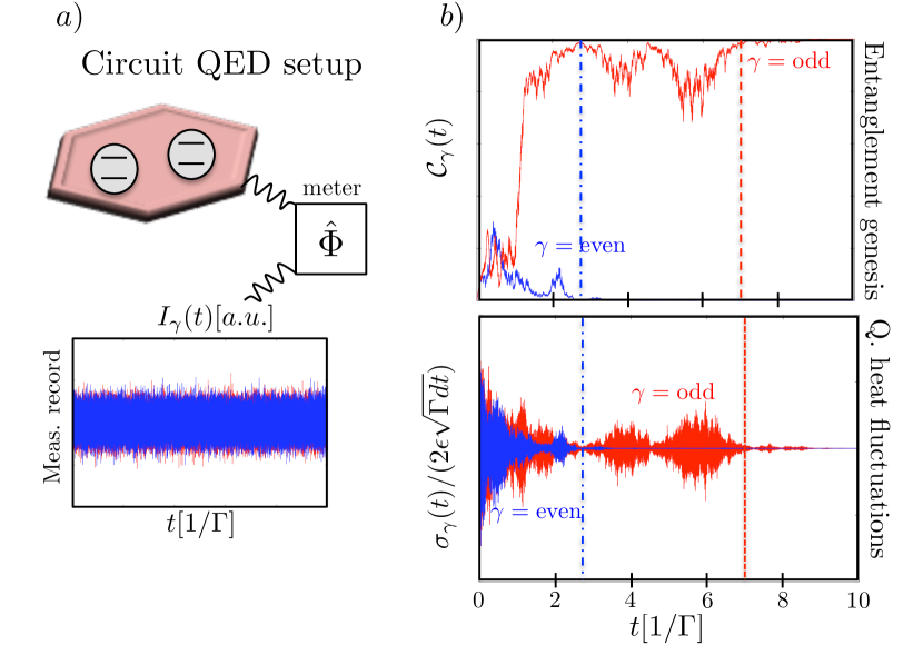
In addition, the qubits are subject to a weak continuous measurement of the joint observable , that implements a half-parity measurement, see Fig. 1. Within the two-qubit computational basis , the collective operator is defined by and has three eigenvalues and with eigenstates , and respectively. The eigenvalue 0 is degenerate, implying that this outcome does not allow one to distinguish between the two odd states . Consequently, when outcome is obtained from the measurement, the two qubits are driven into a coherent superposition of those states, which leads to entanglement. On the contrary, the measurement of the eigenvalues allows to distinguish the two even states, leaving the qubits in a product state. Hence, the half-parity measurement presents the specificity of producing in a probabilistic way entangled and product states. It is clear from the expression of that its measurement does not put the qubits into an entangled state (spanned by the odd states) if these ones are not in a coherent superposition initially. Although the forms of and of the parity operator seem to be specific, these joint operators are the only ones up to local unitary operations that can generate correlations between two qubits. This explains the high interest in the past years for this parity measurement protocol within solid-state setups, also known within the quantum information community as a Bell measurement. This one was for instance proposed and realized for quantum teleportation [2, 27].
Quantum trajectories– Assuming a weak continuous measurement of , each realization of the measurement procedure is associated to a quantum stochastic trajectory followed by the qubits and labelled in the rest of the manuscript [28, 29]. We assume the initial state of the qubits is a known pure state, see Eq.(2), such that the trajectory is made of a sequence of pure states . To each trajectory corresponds a stochastic measurement record :
| (3) |
Here, is the expectation value of the half-parity operator w.r.t. the state , and corresponds to the detector measurement rate, i.e. the rate at which one is able to distinguish the measurement outcomes from the detector’s shot noise [30, 31, 12, 13]. The infinitesimal Wiener increment is a stochastic variable characterized by a zero average and variance , i.e. and , where denotes the average over all realizations of the measurement during the time interval . Note that throughout this work, we use Ito’s convention for stochastic differential calculus [32, 33]. This infinitesimal Wiener increment encodes Gaussian fluctuations of the measurement record around its expectation value and therefore captures the detector’s shot noise in the weak coupling limit [31, 29]. Based upon the knowledge of , the conditional dynamics of the two qubits subject to the weak measurement of the half-parity observable is captured by the stochastic Schrödinger equation
| (4) | |||||
Using , see Eq. (1), one can solve analytically Eq.(4) at any time as a function of the stochastic measurement record:
| (5) |
with the time-dependent normalization factor . Following Ref. [29], this solution is expressed in terms of the measurement outcome :
| (6) |
with a Gaussian random variable with mean zero and variance . The time integral corresponds to a finite resolution time, typically set by experimental constraints. The probability distribution of is a sum of three Gaussian functions of variance , each peaked around one of the eigenvalues of the measured observable :
| (7) |
with the variance setting the measurement strength. In the long time limit , only takes one of three possible outcomes which are the eigenvalues of the half-parity measurement operator: , . At those long times, the measurement becomes projective. In the following of the work, we choose to label the different trajectories with their long-time value of ; this defines three subsets of trajectories, leading the qubits either in an entangled state () or in a product state ().
Measure of entanglement– We quantify the presence of entanglement at any time using the concurrence, a monotone measure for two-qubit entangled states [34]. The qubits being in a pure state at each instant of time along their trajectory , we can make use of a simpler definition where are the amplitudes of with respect to the computational states respectively. Inserting Eq.(5), we get a stochastic concurrence which depends on the measurement outcome :
| (8) |
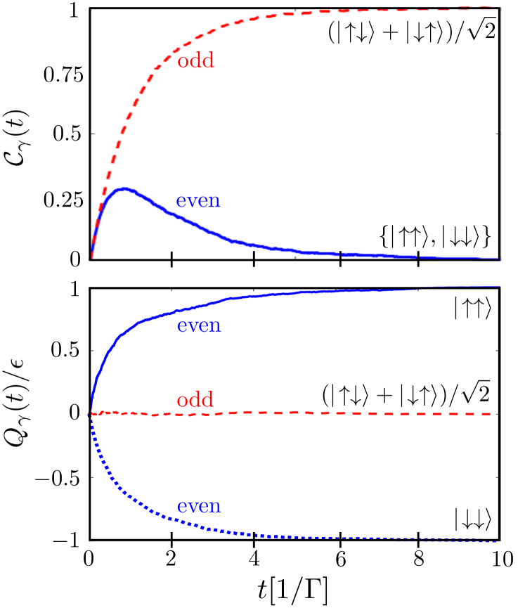
Figure 2 a) shows the time evolution of the average post-selected concurrence according to the three subsets of trajectories, labeled by the final outcomes . The average is made over all realizations that belong to a given subset. At long times, , the concurrence can be directly obtained by replacing in Eq.(8) by the -eigenvalues as the measurement becomes projective. Under optimal conditions as considered here (QND-measurement, no additional dephasing processes, ideal detection scheme), the concurrence reaches the value 1 when qubits are driven into the odd subspace, meaning that the qubits end up in a maximally entangled state. Non-ideal conditions encountered in experiments lead to a lower maximal value of concurrence, and eventually to a long-time state that is separable if dephasing processes are too important. This was for instance the case in Ref. [15], and can be accounted for theoretically.
In this work, the goal is to establish fundamental links between energetic signatures and the generation of entanglement. This is why we focus below on the realization of weak continuous half-parity measurement under optimal conditions. Non-ideal conditions could also be accounted for, but would prevent us to draw clear conclusions on the origin of these energetic signatures.
3 Half-parity measurement seen as an energy measurement (filter)
It is remarkable that the half-parity observable also serves as energy filter within our model: , both being related by the energy gap of the qubits (see Eq. (1)). Hence, the half-parity measurement provides a direct access to the energetics of the qubits along the quantum trajectories generated by the weak measurement of . The internal energy of the two qubits along a given trajectory is given by:
| (9) |
Considering the initial state (see Eq.(2)), the initial internal energy is zero and constitutes the energy reference. In the absence of driving, is time-independent. Hence no work is performed onto the qubits. In addition, there is no thermal reservoir involved in the problem so that a change in the internal energy of the qubits can only arise from the measurement process itself. This form of energy exchange has no classical counter-part [35, 25, 23, 36, 37, 38] and will be, in the line of [23], referred to as quantum heat and denoted in this article.
Long times: projective energetic measurement– At long times, , the change of internal energy (associated here to a net quantum heat ) takes three different values depending on the measurement outcomes:
| (13) |
When averaged over all trajectories, , which equals the reference internal energy at initial time . This equality follows from that characterizes a QND-measurement. Indeed, as both observables commute, there must be no change of internal energy on average and this must hold at all times. At long times, the weak continuous measurement of is equivalent to a projective energy measurement, and this explains the long-time values of for the different subsets of trajectories, equal to the energy of the odd states and even states and respectively.
Intermediate times– At arbitrary time , the quantum heat exchange depends on the exact outcome :
| (14) | |||||
This quantum heat exchange , after post-selection, is plotted in Fig. 2 b) as a function of time. As for the concurrence, an average is made within each subset of trajectories defined by the long-time limit value of the measurement record . Because the half-parity measurement amounts to an energetic measurement, an access to the internal energy is sufficient to determine whether the qubits are entangled or not. A record equal to 0 implies that the qubits ended up in the odd subspace, in a coherent superposition of the odd states .
This first part demonstrates that, on top of being a way to generate entangled state in a heralded way (the outcome is enough to know whether the final state is entangled) as demonstrated in previous works, the half-parity measurement also gives access to the joint internal energy of the qubits. Let us note that the rate at which the quantum heat exchange converges to its final value corresponds to the measurement-induced dephasing rates derived in previous works [12, 13, 14, 15].
Stochastic fluctuations at arbitrary times– To derive the fluctuations of the quantum heat, let us first introduce the increment that corresponds to the stochastic infinitesimal variation of the internal energy between times and along a trajectory . It is related to the total quantum heat exchange up to time via:
| (15) |
and is defined as
| (17) | |||||
Inserting Eqs. (1) and (5) into Eq. (17) and expanding the last term up to the first order in , we obtain
| (18) | |||||
with
| (19) | |||||
| (20) |
Here, we have introduced the populations for the 4 two-qubit states defined as and we denote and the populations within the even and odd parity subspaces respectively. From those definitions, the products and correspond respectively to the squared coherences (off-diagonal elements in the two-qubit density matrix) within the even subspace and between the even and odd subspaces. Let us recall that a (half-) parity measurement generates entanglement by distinguishing the even states form the odd ones. It is therefore the loss of coherence between the two parity subspaces that brings the two qubits in a coherent superposition of odd states when outcome is obtained. Hence, we claim that the product (equivalently ) in Eq.(20) reflects entanglement genesis, and so does the total heat increment . We demonstrate this claim in the following sections.
4 Energetic bounds for the entanglement genesis rate
To validate our claim, we define the standard deviation of the quantum heat increment between times and as
| (21) | |||||
where we made use of and . For simplicity, we will work in the following with dimensionless quantities:
| (22) |
refers to the variance of the Gaussian distribution of the measurement record during the discrete time interval , see the variance defined in Eq. (7). Similarly to Eq. (18), we define two contributions to the standard deviation of the stochastic quantum heat increment:
| (23) |
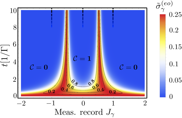
Figure 3 illustrates our claim. The contour plot corresponding to constant values of the concurrence is superimposed onto the density plot of . It highlights that an increase in the concurrence is associated with non-zero fluctuations of . In contrast, the concurrence plateaus correspond to the areas where vanishes. This observation is supported by a strict equality between the concurrence variation (the concurrence derivative) and for the trajectories leading the qubits into an entangled state (see App. A for detailed derivation):
| (24) |
Because it constitutes at the same time the source of entanglement and a direct access to the energy and its fluctuations, it follows that the energy fluctuations must be related to the creation of entanglement. However, the practical interest of Eq. (24) is limited as it would be impossible in a heat-sensitive measurement to distinguish the two contributions and .
Nevertheless, at intermediate times, we demonstrate that the concurrence derivative, that characterizes the rate at which entanglement is induced by the measurement, can be upper and lower bounded by energetic quantities solely. Starting from
we then perform an an ensemble average over all trajectories (or equivalently over the measurement record ) during the time interval , keeping the past records fixed. This interval is the one over which we investigate the fluctuations of the quantum heat increment , and this ensemble average corresponds to the one used in the definitions of the quantum heat increment fluctuations, see Eq.(21). We then have in Eq.(4) and
Inequalities (27) and (28) constitute one of the main analytical results of this work. The entanglement rate is exclusively upper and lower bounded by energetic quantities, the quantum heat and quantum heat fluctuations defined in Eq.(22). All quantities are defined over a (small) finite time interval . Remarkably, we can further exploit Ineq. (27) towards the derivation of an energetic-based estimator to assess the presence of entanglement at intermediate times. Of interest towards single shot entanglement detection, this will be done at the level of a unique quantum trajectory.
5 Single-shot energetic-based estimator for entanglement
Formally, a witness for entanglement is an observable that takes a negative value when averaged with respect to a state that is entangled. If the witness takes a positive value, no conclusions can be drawn, the state can either be entangled or separable [39]. In the past years, few witnesses based on temperature have been proposed, as a first attempt to exploit energetic quantities to certify the presence of entanglement [40, 41]. Following the spirit of assessing the presence of entanglement with some independent quantities, we introduce in this section a trajectory-based witness, i.e. a quantity which takes negative value in presence of entanglement, just as usual entanglement witnesses, but which takes as an input a single quantum trajectory, or equivalently a weak measurement record, instead of a quantum state. As a first step to build this witness, we use the property that a given quantum trajectory will drive the qubits onto an entangled state if,
| (29) |
This condition is motivated by the idea that accumulating positive time-derivatives would lead to a positive concurrence at final time . While one cannot certify the presence of entanglement along individual trajectory from Eq.(29), the integration over time of used to compute the concurrence at time is expected to play the role of the ensemble average for and provided . Therefore, condition (29) implies an entangled state at time for a high fraction of the considered trajectories.
Making use of inequality (27), this condition translates into:
| (30) |
We can now use that the concurrence takes values within to prove an inequality assessing the presence of entanglement, that only depends on energetic quantities, We can now directly use this condition to introduce our trajectory-based entanglement witness , defined as:
| (31) |
The time-averaged over is meant to take into account a finite acquisition time during the experiment. When is negative, one can expect with high probability that the trajectory leads to qubits in an entangled state. When it is positive, one can not draw a definite conclusion. However, and as stated before, this quantity implies an ensemble-average over all trajectories occurring during the finite time interval , which is not yet optimal for experimental purposes. We therefore define an estimator (with the label referring to single-shot), where the ensemble average in the definition of Eq.(21) is replaced by a time average over an interval . This procedure is similar to a coarse-graining of the fluctuations along a single trajectory. The witness (31) then transforms into an estimator, valid at the level of single trajectory:
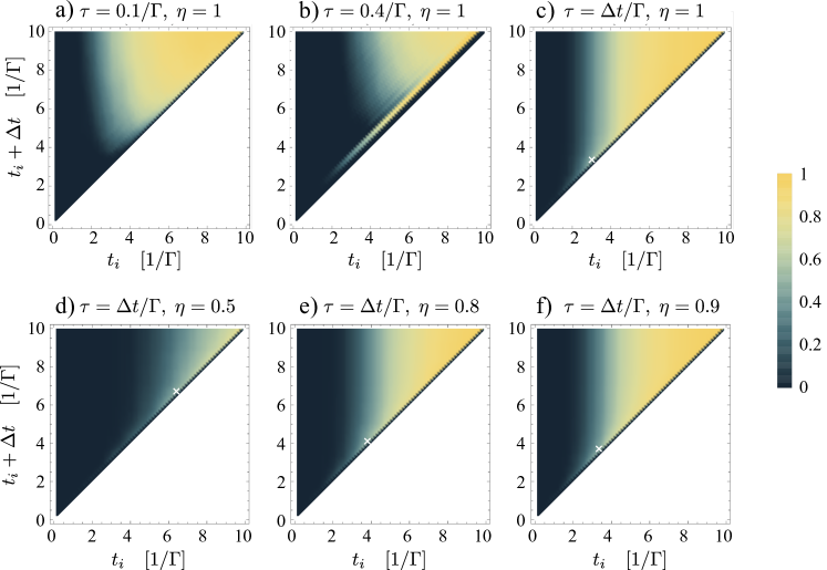
The performance of as an estimator to attest entanglement between the qubits is analyzed through two figures of merit, its success rate (ratio of detected vs. total number of trajectories leading to entangled states) and its error rate (whenever takes a negative value whereas the trajectory does not lead to entangled qubits). The error rate takes the maximal value of for the coarse-graining times and and for . Indeed, as the coarse-graining time increases, the time average leads to trusty measurements, as expected from the analytical bound derived with the ensemble-averaged. The finite error rate forbids us to claim an energetic witness, but its small value demonstrates the usefulness of our energetic-based estimator. As shown in Fig.4, the success rate of does not strongly depend on the overall integration window , but rather on the initial time from which the averages are performed. At large , the success rate reaches 1 as expected from the convergence of each trajectory towards one of the eigenstate of the measurement operator . However, the success rate exceeds 0.5 for as small as for , with a corresponding error rate of , being promising for future experiments towards single-shot energetic-based estimators to certify the presence of entanglement. Finally, as a first step towards realistic implementation, we have also investigated the robustness of our estimator against finite detection efficiency. We have numerically simulated trajectories when the half-parity detection channel has an efficiency , which leads to mixed state trajectories [29], see App. C . As a consequence, the analytic justification for the estimator is not valid anymore as the formula for the concurrence has to be modified for mixed state[34] and there is no analytic expression for the state conditioned to a given readout . However, a numerical treatment is possible, and it is straightforward to extend the definition (5) to mixed state trajectories, using the average heat increment along mixed state trajectory defined as . The latter is related to the populations of the states and and of the even and odd subspaces in the same way as in Eq.(18), with an additional overall factor . The generation of entanglement happens to be quite robust to finite detection efficiency, as witnessed by the experimental implementations [14, 15]. The success rate, computed from a sample of numerically generated trajectories, is plotted for finite efficiency in Fig. 4d)-f) for different values of , showing that our method is robust against finite detection efficiency. High success rates (up to for ) are predicted even for which is the order of magnitude of the experimental conditions. The error rate remains smaller or of the order of .
6 Discussion
In this work, we investigate the energy fluctuations associated with entanglement genesis during the paradigmatic half-parity measurement procedure. Not only this measurement generates both product states and entangled states, but it also constitutes an energy observable. Based on a quantum-trajectory approach, and making use of the framework provided by stochastic thermodynamics, we demonstrate that the generation of entanglement is closely related to the presence of quantum heat fluctuations induced by the stochasticity of the weak continuous measurement. We derive analytical upper and lower bounds for the entanglement genesis rate. We then exploit the lower bound to derive an estimator that is solely based on energetic observables and their fluctuations. We show that this energetic-based estimator is indeed able to attest the presence of entanglement at a finite time for a given quantum trajectory, with a tunable probability that depends on the total time-averaged window . Remarkably, this single-shot estimator is valid at the level of a single trajectory and so does not require any ensemble average. Remarkably, the energetic-based estimator we proposed is robust to finite detection efficiency, reaching a success rate close to 1 for suitable integration times as discussed earlier.
These results do not aim at evaluating the energetic cost of creating quantum correlations, see for instance Refs.[42, 43, 44], but rather at defining an energetic signature associated to their generation. Whereas the quantum heat is zero on average, the quantum fluctuations during a finite time interval contain relevant information to attest the presence of entanglement.
Exact in the context of the half-parity measurement process which also plays the role of an energetic filter, our work fixes theoretical tools for thermodynamic analysis of the generation of quantum correlations and opens the way to develop witnesses based exclusively on the measurements of energetic quantities for quantum information purposes. This theoretical research is additionally motivated by recent experimental achievements in the emergent field of quantum caloritronics, aiming at controlling and measuring energetic observables like the heat current in various quantum circuits [45, 46, 47, 48, 49, 50, 51].
Acknowledgements G.H. gratefully acknowledges discussions with J. Anders, A. Jordan and I. Siddiqi. C.E. acknowledges the US Department of Energy grant No. DE-SC0017890. This research was supported in part by the National Science Foundation under Grant No. NSF PHY-1748958. G.H. thanks the Swiss National Science Foundation for support through the MHV grant 164466 and starting grant PRIMA PR00P2179748. This research was supported in part by the National Science Foundation under Grant No. NSF PHY17-48958.
Appendix A Long-time limit formula between the concurrence derivative and infinitesimal heat fluctuations
The fluctuations of the heat increment associated to the lose of coherences between the two parity subspaces are defined in a similar was as :
| (33) | |||||
| (34) |
We can compare them to the derivative of the concurrence averaged over realizations occurring during the time interval :
| (35) | |||||
When , the probability distribution of the measurement outcome is narrowly peaked around the three values corresponding to the eigenvalues of the half-parity measurement operator [29], i.e. . The average value of tends also to one of the three eigenvalues. Hence, for trajectories corresponding to qubits in a maximally entangled state at long times, and the heat flow . Consequently, Eqs. (34) and (35) simplify to
| (36) | |||||
| (37) |
When time exceeds the measurement time, the following equality holds:
| (38) |
Although only valid and meaningful at times longer than the measurement time, this relation exemplifies the underlying fundamental role of infinitesimal heat fluctuations for the generation of entanglement. As stated in the main text, this relation is only exact in the context of the half-parity measurement considered in this work and can not be exploited experimentally. Indeed, one could not distinguish in an experiment infinitesimal heat fluctuations originating in the loss of phase coherence between the two parity subspaces () from total infinitesimal heat fluctuations ().
Appendix B Energetic bounds for the entanglement genesis rate
Appendix C Finite detection efficiency
When the efficiency of the detector takes a finite value , the state of the two qubits along a given trajectory is a mixed state which obeys [29]:
| (45) |
where . The measurement record is now linked to the Wiener increment via:
| (46) |
References
- Ekert [1991] A. K. Ekert, Phys. Rev. Lett. 67, 661 (1991).
- Bennett et al. [1993] C. H. Bennett, G. Brassard, C. Crépeau, R. Jozsa, A. Peres, and W. K. Wootters, Phys. Rev. Lett. 70, 1895 (1993).
- Briegel et al. [1998] H.-J. Briegel, W. Dür, J. I. Cirac, and P. Zoller, Phys. Rev. Lett. 81, 5932 (1998).
- Raussendorf and Briegel [2001] R. Raussendorf and H. J. Briegel, Phys. Rev. Lett. 86, 5188 (2001).
- Nielsen M. [2010] C. I. Nielsen M., Quantum Computation and Quantum Information: 10th Anniversary Edition (Cambridge: Cambridge University Press, 2010).
- Lalumière et al. [2010] K. Lalumière, J. M. Gambetta, and A. Blais, Phys. Rev. A 81, 040301 (2010).
- Tornberg and Johansson [2010] L. Tornberg and G. Johansson, Physical Review A 82, 012329 (2010).
- Chantasri et al. [2016] A. Chantasri, M. E. Kimchi-Schwartz, N. Roch, I. Siddiqi, and A. N. Jordan, Phys. Rev. X 6, 041052 (2016).
- Royer et al. [2018] B. Royer, S. Puri, and A. Blais, Science Advances 4, eaau1695 (2018).
- Trauzettel et al. [2006] B. Trauzettel, A. N. Jordan, C. W. J. Beenakker, and M. Büttiker, Phys. Rev. B 73, 235331 (2006).
- Williams and Jordan [2008] N. S. Williams and A. N. Jordan, Phys. Rev. A 78, 062322 (2008).
- Haack et al. [2010] G. Haack, H. Förster, and M. Büttiker, Phys. Rev. B 82, 155303 (2010).
- Meyer zu Rheda et al. [2014] C. Meyer zu Rheda, G. Haack, and A. Romito, Phys. Rev. B 90, 155438 (2014).
- Ristè et al. [2013] D. Ristè, M. Dukalski, C. A. Watson, G. de Lange, M. J. Tiggelman, Y. M. Blanter, K. W. Lehnert, R. N. Schouten, and L. DiCarlo, Nature 502, 350 (2013).
- Roch et al. [2014] N. Roch, M. E. Schwartz, F. Motzoi, C. Macklin, R. Vijay, A. W. Eddins, A. N. Korotkov, K. B. Whaley, M. Sarovar, and I. Siddiqi, Phys. Rev. Lett. 112, 170501 (2014).
- Weber et al. [2014] S. J. Weber, A. Chantasri, J. Dressel, A. N. Jordan, K. W. Murch, and I. Siddiqi, Nature 511, 570 (2014).
- Ficheux et al. [2017] Q. Ficheux, S. Jezouin, P. Campagne-Ibarcq, P. Rouchon, and B. Huard, in Quantum Information and Measurement (QIM) 2017 (Optical Society of America, 2017) p. QF5A.2.
- Naghiloo et al. [2018] M. Naghiloo, J. J. Alonso, A. Romito, E. Lutz, and K. W. Murch, Phys. Rev. Lett. 121, 030604 (2018).
- Elouard et al. [2017a] C. Elouard, D. Herrera-Martí, B. Huard, and A. Auffèves, Phys. Rev. Lett. 118, 260603 (2017a).
- Elouard and Jordan [2018] C. Elouard and A. N. Jordan, Phys. Rev. Lett. 120, 260601 (2018).
- Buffoni et al. [2018] L. Buffoni, A. Solfanelli, P. Verrucchi, A. Cuccoli, and M. Campisi, (2018), arXiv:1806.07814.
- Ding et al. [2018] X. Ding, J. Yi, Y. W. Kim, and P. Talkner, Phys. Rev. E 98, 042122 (2018).
- Elouard et al. [2017b] C. Elouard, D. A. Herrera-Martí, M. Clusel, and A. Auffèves, npj Quantum Information 3, 9 (2017b).
- Manzano et al. [2015] G. Manzano, J. M. Horowitz, and J. M. R. Parrondo, Phys. Rev. E 92, 032129 (2015).
- Alonso et al. [2016] J. J. Alonso, E. Lutz, and A. Romito, Phys. Rev. Lett. 116, 080403 (2016).
- Elouard and Mohammady [2018] C. Elouard and H. Mohammady, Work, heat and entropy production along quantum trajectories (2018) arXiv:1805.08305.
- Riebe et al. [2004] M. Riebe, H. Häffner, C. F. Roos, W. Hänsel, J. Benhelm, G. P. T. Lancaster, T. W. Körber, C. Becher, F. Schmidt-Kaler, D. F. V. James, and R. Blatt, Nature 429, 734 EP (2004).
- Wiseman [1996] H. M. Wiseman, Quantum and Semiclassical Optics: Journal of the European Optical Society Part B 8, 205 (1996).
- Jacobs and Steck [2006] K. Jacobs and D. A. Steck, Contemporary Physics 47, 279 (2006).
- Pilgram and Büttiker [2002] S. Pilgram and M. Büttiker, Phys. Rev. Lett. 89, 200401 (2002).
- Korotkov [1999] A. N. Korotkov, Phys. Rev. B 60, 5737 (1999).
- Gardiner [1985] C. Gardiner, Handbook of Stochastic Methods (Springer-Verlag Berlin Heidelberg, 1985).
- Gillespie [1996] D. T. Gillespie, American Journal of Physics 64, 225 (1996).
- Wootters [1998] W. K. Wootters, Phys. Rev. Lett. 80, 2245 (1998).
- Brandner et al. [2015] K. Brandner, K. Saito, and U. Seifert, Phys. Rev. X 5, 031019 (2015).
- [36] K. Abdelkhalek, Y. Nakata, and D. Reeb, Fundamental energy cost for quantum measurement, ArXiv:1609.06981.
- Elouard et al. [2017c] C. Elouard, D. Herrera-Martí, B. Huard, and A. Auffèves, Physical Review Letters 118, 260603 (2017c).
- Yi et al. [2017] J. Yi, P. Talkner, and Y. W. Kim, Phys. Rev. E 96, 022108 (2017).
- Plenio and Virmani [2007] M. B. Plenio and S. Virmani, Quantum Info. Comput. 7, 1 (2007).
- Anders et al. [2006] J. Anders, D. Kaszlikowski, C. Lunkes, T. Ohshima, and V. Vedral, New Journal of Physics 8, 140 (2006).
- Anders [2008] J. Anders, Phys. Rev. A 77, 062102 (2008).
- Huber et al. [2015] M. Huber, M. Perarnau-Llobet, K. V. Hovhannisyan, P. Skrzypczyk, C. Klöckl, N. Brunner, and A. Acín, New Journal of Physics 17, 065008 (2015).
- Bruschi et al. [2015] D. E. Bruschi, M. Perarnau-Llobet, N. Friis, K. V. Hovhannisyan, and M. Huber, Phys. Rev. E 91, 032118 (2015).
- Friis et al. [2016] N. Friis, M. Huber, and M. Perarnau-Llobet, Phys. Rev. E 93, 042135 (2016).
- Giazotto and Martínez-Pérez [2012] F. Giazotto and M. J. Martínez-Pérez, Nature 492, 401 (2012).
- Jezouin et al. [2013] S. Jezouin, F. D. Parmentier, A. Anthore, U. Gennser, A. Cavanna, Y. Jin, and F. Pierre, Science 342, 601 (2013).
- Gasparinetti et al. [2015] S. Gasparinetti, K. Viisanen, O.-P. Saira, T. Faivre, M. Arzeo, M. Meschke, and J. Pekola, Physical Review Applied 3, 014007 (2015).
- Iftikhar et al. [2016] Z. Iftikhar, A. Anthore, S. Jezouin, F. D. Parmentier, Y. Jin, A. Cavanna, A. Ouerghi, U. Gennser, and F. Pierre, Nature Communications 7, 12908 (2016).
- Fornieri and Giazotto [2017] A. Fornieri and F. Giazotto, Nature Nanotechnology 12, 944 (2017).
- Banerjee et al. [2017] M. Banerjee, M. Heiblum, A. Rosenblatt, Y. Oreg, D. E. Feldman, A. Stern, and V. Umansky, Nature 545, 75 (2017).
- van Zanten et al. [2016] D. M. T. van Zanten, D. M. Basko, I. M. Khaymovich, J. P. Pekola, H. Courtois, and C. B. Winkelmann, Phys. Rev. Lett. 116, 166801 (2016).
