Development of a Sensory-Neural Network for Medical Diagnosing

Abstract

Performance of a sensory-neural network developed for diagnosing of diseases is described. Information about patient’s condition is provided by answers to the questionnaire. Questions correspond to sensors generating signals when patients acknowledge symptoms. These signals excite neurons in which characteristics of the diseases are represented by synaptic weights associated with indicators of symptoms. The disease corresponding to the most excited neuron is proposed as the result of diagnosing. Its reliability is estimated by the likelihood defined by the ratio of excitation of the most excited neuron and the complete neural network.

Keywords: sensory-neural network, disease symptoms, medical diagnosing.

1 Introduction

Medical diagnosing can be treated as a mapping of symptoms to characteristics of diseases [1, 2]. Our goal is to develop a sensory-neural network (SNN) by which this mapping could be performed automatically by a PC [3, 4, 5]. With this aim we first transform data about patient’s condition into a proper form for the numerical processing. This transformation corresponds to sensing of symptoms by sensors at the input layer of the SNN shown in Fig. 1. Similarly as data of patients, the characteristics of diseases are transformed and utilized to specify the synaptic weights of neurons in the next layer [6]. At this specification we take into account the performance of a doctor at the diagnosis assessment.

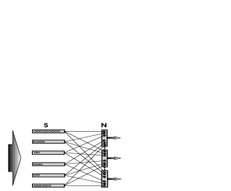
Figure 1: Schematic drawing of the sensory-neural network. Bold arrows demonstrate input and output information flow, o - denote symptom indicators, ${\bf\ast}$ - show synapses, $\leftrightarrow$ - represent connections between SNN elements.

The doctor collects symptoms of the treated patient and compares them with the properties of diseases. At the comparison he considers certain symptoms as more significant than others and so assesses the agreement between given symptoms and those describing diseases [6, 7]. The disease with the highest correlation is then selected as a result of diagnosis. We describe such treatment by characterizing the significance of symptoms by synaptic weights connecting the sensors to neurons that correspond to various diseases. A signal from a particular sensor thus contributes different amounts to excitation of various neurons. The excitation of a particular neuron therefore represents the correlation between the symptoms of a patient and the properties of the disease represented by the neuron. The disease corresponding to the most excited neuron in the NN layer determines the result of diagnosis. We describe the reliability of such assessment by expressing the output of the neuron relatively with respect to the mean value of all outputs. The corresponding estimator represents the likelihood of the diagnosis. At the specification of the SNN we first select a set of diseases and specify their symptoms as well as synaptic weights of neurons. In terms of them we next define the agreement and likelihood estimators.

Table 1: Symptoms used for characterization of diseases

$s$	Symptom name - $S(s)$	$s$	Symptom name - $S(s)$	$s$	Symptom name - $S(s)$
1	no symptoms	17	sleep disturb.- night walk	33	difficulty when speaking
2	sudden onset of illness	18	distorted vision	34	difficulty moving one side
3	hyperthermia	19	frequent urination	35	sudden infertility
4	malaise, tiredness	20	tinnitus	36	difficult verbal expression
5	age over 70	21	bleeding	37	vomiting
6	headache	22	dark urine in last 2 weeks	38	snoring during sleep
7	sudden headache	23	thirst, dry mouth	39	smelly urine
8	cough	24	nervousness, depression	40	heart rate
9	dizziness	25	throat irritation	41	arterial hypertension
10	trouble breathing	26	pharyngeal dryness	42	pulse rhythmicity
11	pain	27	hoarseness	43	O satur. - pulse oxim.
12	w. loss in last 1/2 y	28	obstruction in the throat	44	breathing frequency
13	loss of appetite	29	jaundice of skin & sclera	45	body height
14	irregular pulse	30	light feces	46	body weight
15	sweating	31	frequent infections
16	difficult concentrating	32	ability to lift both arms

Table 2: Indicators of symptoms

$s$	Indicators $I(s,:)$
3	{fever, y, n}
6	{y, n, in the morning, daily persistent}
8	{y-in the morning, y-with sputum, y-daily persistent, y-without sputum,n}
10	{at rest, on exertion, n}
11	{chest,ear,abdomen,pharynx,at swallowing,at speaking,at urinating,shoulder,n}
15	{daily persistent, nocturnal,n}
18	{y, n, one eye only}
19	{y, n, at night}
21	{from the nose, in the sputum, in the urine, n}
31	{urinary tract, tongue, corners of the mouth, lung, n}
40	{$<$50, 51-70, 71-90, $>$90}
41	{$<$100, 100-140, $>$140}
42	{rhythmic, arrhythmic}
43	{$\leq$ 90, $>$90}
44	{$<$10, 11-15, $>$15}
45	{$<$150, 151-160, 161-170, 171-180, 181-190, $>$190} cm
46	{$<$50, 51-60, 61-70, 71-80, 81-90, 91-100, $>$100} kg

All other possible indicators are specified by: $I(s,:)=\{{\rm yes,no}\}=\{{\rm y,n}\}$.
Components missing in Table 2 correspond to empty space $\emptyset$, for example: $I(s,:)=\{{\rm fever,y,n}\}\equiv\{{\rm fever,y,n,\emptyset,\emptyset,\emptyset,\emptyset,\emptyset,\emptyset}\}$.

2 Properties of data bases

2.1 Symptoms and diseases

According to the suggestion of the research initiator [5] we apply the set of $15$ most frequent diseases denoted by the name and index $D(d)$: 1) Anemia, 2) Urinary tract infection, 3) Diabetes-2, 4) Atrial fibrillation, 5) Acute hemorrhagic stroke, 6) Obstructive sleep apnea, 7) Tuberculosis, 8) Chronic obstructive pulmonary disease, 9) Pneumonia, 10) Otitis media, 11) Leukocytosis, 12) Hepatitis-A, 13) Hypertension, 14) Throat inflammation, 15) No disease. Their properties are characterized by $N_{s}=46$ symptoms $S(s)$ shown in Table 1 and used to describe the sensory layer of the SNN [3, 4]. A symptom $S(s)$ is described by up to $N_{i}=9$ possible indicators $I(s,i)$ shown in Table 2.

A particular disease is characterized by various symptom indicators. The presence or absence of a symptom indicator can be generally denoted by $0$ or $1$, but such indication leads to a very rough assessment of diagnosis. For a better assessment we describe the importance of the symptom indicator $I(s,i)$ of the disease $D(d)$ by a synaptic weight $W(d,s,i)$. A non important indicator is assigned the weight $W=0$, while the other weights are positive or negative. A negative weight points to the absence of the disease. To avoid problems related with network training we apply a set of fixed weights specified by a clinical research. Their values mostly lie in the interval (1, 3).

Table 3: Statistical weights describing importance of symptom indicators

$d$	The values denote: (symptom index $s$, indicator index $i$, weight $W(d,s,i)$)
1	(2,2,1) (3,3,1) (4,1,1) (6,1,1) (9,1,1) (10,1,1) (14,1,1) (16,1,1) (17,1,1) (20,1,1)
	(31,1,1) (31,3,2) (40,4,1) (44,3,2)
2	(2,1,1) (3,1,3) (3,2,1) (11,3,2) (11,8,4) (19,1,3) (22,1,3) (39,1,3)
3	(2,2,2) (3,3,2) (4,1,1) (12,2,2) (18,1,1) (19,1,2) (31,1,2)
4	(2,1,3) (3,2,3) (5,1,3) (10,2,2) (11,1,2) (14,1,3) (41,2,1) (41,3,3) (42,2,3)
5	(2,1,2) (3,3,1) (7,1,2) (9,1,1) (18,3,2) (32,2,2) (33,1,2) (34,2,2) (35,1,2) (36,1,2)
	(37,1,1)
6	(2,2,1) (4,1,1) (6,3,1) (16,1,1) (17,1,3) (23,1,1) (24,1,2) (41,3,1) (46,6,2) (46,7,3)
7	(2,2,1) (3,2,1) (4,1,1) (8,3,3) (11,1,1) (12,1,1) (13,1,1) (15,2,3) (21,2,3)
8	(2,2,2) (3,3,1) (8,1,3) (8,2,3) (8,5,-3) (31,4,2)
9	(2,1,2) (3,1,3) (3,2,1) (4,1,2) (8,2,1) (8,3,1) (8,4,1) (10,1,1) (10,2,1) (11,1,1)
10	(2,1,2) (3,2,1) (4,1,1) (6,4,2) (11,2,3) (29,1,1)
11	(2,2,1) (3,2,1) (4,1,1) (9,1,1) (10,1,1) (10,2,1) (12,1,1) (13,1,1) (15,1,1) (18,1,1)
12	(2,1,2) (3,2,1) (4,1,3) (11,3,2) (13,1,2) (29,1,3) 22,1,3) (30,1,3) (37,1,2)
13	(2,2,1) (3,3,2) (5,1,1) (6,4,2) (9,1,1) (21,1,1) (41,3,6)
14	(2,1,2) (3,1,1) (11,4,3) (25,1,2) (26,1,1) (27,1,1) (28,1,1)
15	(1,1,1) (2,2,1) (3,3,1) (4,2,1) (6,2,1) (8,5,1) (11,9,1) (13,2,1) (16,2,1) (18,2,1)
	(21,4,1) (22,2,1) (23,2,1) (24,2,1) (25,2,1) (26,2,1) (27,2,1) (28,2,1) (29,2,1)
	(30,2,1) (31,5,1) (32,2,1) (33,2,1) (34,2,1) (35,2,1) (36,2,1) (37,2,1) (38,2,1)
	(39,2,1)

Weights at other indices are $0$.

By the set $\{W(d,s,i);1\leq d\leq 15;1\leq s\leq 46;1\leq i\leq 9\}$ shown in Table 3 we describe quantitatively the properties of diseases. For this purpose we treat the weights $W(d,s,i)$ as the transmission parameters of synaptic joints on the neuron with index $d$. To provide for equivalent treatment of all diseases at the assessment of a diagnosis, it is reasonable to normalize the weights so that the sum of their positive values equals $1$. By using the Heaviside function: $\{H(x)=0$ for $x\leq 0$ ; $H(x)=1$ for $x>0\}$ we include just positive weights into the total positive weight: $W_{t}(d)=\sum_{s=1}^{N_{s}}\sum_{i=1}^{N_{i}}W(d,s,i)H(W(d,s,i))$, and define the normalized weight by the fraction: $W_{n}(d,s,i)=W(d,s,i)/W_{t}(d)$.

2.2 Algorithm of diagnosis

At a diagnosis, the patient first completes the questionnaire containing names of symptoms and their indicators. A confirmed item is represented by the value $1$ in the response matrix $\{R(s,i);s=1\ldots N_{s};i=1\ldots N_{i}\}$, while all other non-confirmed terms are $0$. This matrix represents the signals of values $0/1$ supplied from the sensory to neural layer of the network. We next assume that the signal from $I(s,i)$ excites the $neuron(d)$ over the synaptic weight $W_{n}(d,s,i)$ and adds to its output the amount $W_{n}(d,s,i)R(s,i)$. The complete output of the $neuron(d)$ is then given by the sum:

$$A(d)=\sum_{s=1}^{N_{s}}\sum_{i=1}^{N_{i}}W_{n}(d,s,i)R(s,i)$$ (1)

The distribution $\{A(d);d=1,\ldots,N_{d}\}$ describes the excitation of the complete NN, while $A(d)$ is the estimator of the agreement between the patient’s symptoms and the symptoms of the disease $D(d)$. If all symptoms of $D(d)$ coincide with the symptoms confirmed by the patient, the $neuron(d)$ is maximally excited and we get $A(d)=1$ (or $100\%$). As the result of the diagnosis assessment, we propose the disease $D(d_{o})$ with the maximal agreement: $A(d_{o})={\rm max}\,\{A(d);d=1\ldots N_{d}\}$.

To support our decision we determine the mean value $<A>=\sum_{d=1}^{N_{d}}A(d)/N_{d}$ and the standard deviation $\sigma_{A}=\sqrt{{\rm var}(A)}$ of $A(d)$, and then determine the relative deviation: $\Delta_{A}(d)=(A(d)-<A>)/\sigma_{A}$. In the case when $\Delta_{A}(d_{o})\gg 1$ we conclude that the corresponding $D(d_{o})$ is significantly outstanding and can be considered as a reliable quantitative result of the diagnosis. Such reasoning is possible when the symptoms of a particular disease are well exhibited. However, this is not always the case, since several diseases share similar symptoms. This leads to similar stimulations and consequently, a question arises as how to infer when $\Delta_{A}(d_{o})$ is not outstanding. To address this possibility we divide $A(d)$ by the sum: $\sum_{d=1}^{N_{d}}A(d)$ and define the disease likelihood estimator $L(d)$ as:

$$L(d)=\frac{A(d)}{\sum_{d^{\prime}=1}^{N_{d}}A(d^{\prime})}$$ (2)

This estimator describes the relative stimulation of the $neuron(d)$ in the layer of neurons and represents the reliability of our decision. A high value of $L(d)$ corresponds to a firm argument for selecting the corresponding disease as a reliable result of the diagnosis. It is important that both $A(d)$ and $L(d)$ are quantitative in character and thus can be treated as the supplement of other quantitative data in clinical tests.

3 Performance of SNN

3.1 Characterization of the performance

For a wide application we have developed a program that interacts with a user over a graphic interface [3, 4]. At the start the graphic interface presents the user with three options: 1) Identifying a diagnosis based on completing the questionnaire, 2) Testing the program performance based on internally stored data sets of formal symptoms for all diseases, 3) Changing the weights of symptom indicators. All options can be repeated.

In the first option a new window with instructions for the user appears together with a window to enter the patient’s name. After accepting the name, the program shows sequentially $46$ windows with the symptom names and their indicators. Confirmed data are translated into the response matrix $R$ that is led from the sensory to the neural layer of SNN, where the distributions of the agreement $A$ and likelihood $L$ are determined. The results are transferred to the user over various channels. The most informative is the displayed diagram of $A(d)$ and $L(d)$ distribution versus the disease index $d$. The lines at the levels of $<A>$, $<A>+\sigma_{A}$ and $<A>+2\sigma_{A}$ are used as references for a visual assessment of the diagnosis. Two examples are shown in Fig. 2. In addition to such diagram, the files with the patient’s responses and corresponding numerical data are available for printing.

In the second option the program displays the set of diseases. After one of them is selected, the program applies the corresponding formal set of symptoms and uses it instead of the patient’s symptoms in the same procedure as in the first option. This step shows the optimal possibility of the selected disease diagnosis.

The third option allows specialists to examine how a variation of synaptic weights influences the diagnosis process. By adjusting the weights and further testing the diagnosis using the second option, the performance of the complete program can be gradually improved. With this aim, the program allows modification of weights. This option provides for NN training, while the changing of the set of symptoms provides for evolution of the complete SNN.

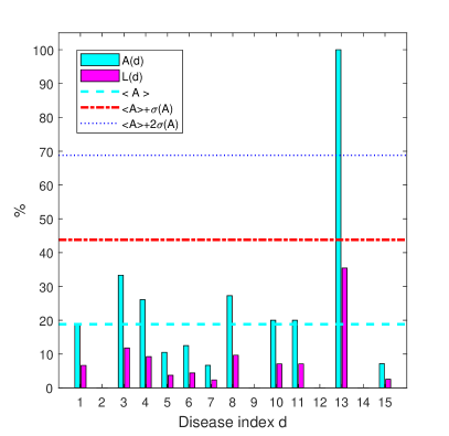
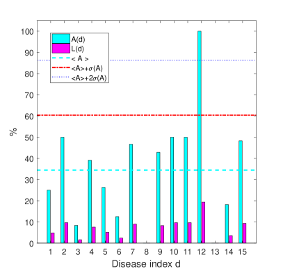
Figure 2: Left : Distribution of $A$ and $L$ in testing the program performance based on formal symptoms of $D(13$) - hypertension. Right : Distribution of $A$ and $L$ based on the answers to the questionnaire by a patient suffering from $D(12)$ - hepatitis A.

3.2 Testing of the program performance

To demonstrate the performance of developed SNN we first present results of its testing performed with the formal symptoms of the typical disease $D(13)$ - hypertension. In this test, we get the diagram shown on the left of Fig. 2.

The value of the corresponding optimal agreement estimator is in this case $A_{o}(4)=100\%$, and it surpasses the mean value $<A>$ for $3.25\,\sigma_{A}$. This outstanding deviation from the mean value indicates a correct assessment of the diagnosis. But the value of $A$ corresponding to several other diseases also surpasses the mean value $<A>$. This outcome indicates that the symptoms of these diseases are in a sense similar to those of hypertension. In spite of this property, the distribution of $A(d)$ suggests selecting hypertension as the result of the diagnosis. Although the agreement with its symptom indicators is $A_{o}=100\%$, the likelihood value of hypertension disease is only $L_{o}=35\%$; the other values, however, are still appreciably smaller: $L(d)\ll L_{o};d\neq d_{o}$.

Similar performance of the program as in testing the diagnosis of hypertension is observed when using formal symptoms of other diseases. The corresponding optimal likelihood values $\{L_{o}(d);d=1,\ldots 15\}$ are:

$$L_{o}=(29,32,34,32,37,33,29,48,24,32,28,28,35,48,41)\%$$ (3)

The mean value of the set of optimal values $\{L_{o}(d);d=1,\ldots,15\}$ is similar as in the demonstrated case of hypertension, amounting to $<L_{o}>=34,6\%$. The corresponding standard deviation is $\sigma_{L}=7\%$ while the maximal and minimal values are $L_{o,max}=L_{o}(8)=L_{o}(14)=48\%$ and $L_{o,min}=L_{o}(9)=24\%$, respectively. These data indicate that the likelihood value of $L_{o}\approx 35\%$ yields a rather firm quantitative argument for accepting the result of the automatic diagnosing.

To demonstrate performance of SNN in the clinical practice we perform diagnosis of the disease $D(12)$ - hepatitis A by data obtained from a patient. The diagram is shown on the right of Fig. 2. In this case the value of the relative agreement is also $A(12)=100\%$ and surpasses the mean value $<A>$ of the agreement distribution by $2.53\,\sigma_{A}$. All other values $\{A(d);d\not=12\}$ are essentially below the value $A(12)$; therefore, we accept as the rather reliable result of diagnosis the $D(12)$ - hepatitis A. This conclusion is supported by the value $L(12)=19\%$ that is smaller as $L_{o}(12)=28\%$ obtained at testing by formal indicators, but still approximately two times greater than all other values. Such result is obtained when all significant symptom indicators in the questionnaire are confirmed by a patient. Other characteristic examples are published elsewhere [3, 4].

4 Conclusions

Our testing has indicated that the selected sets of symptoms and synaptic weights provide a proper basis for the specification of a sensory-neural network applicable for an automatic diagnosing of selected diseases. The advantage of the developed method is the quantitative expression of the agreement between patient symptoms and properties of diseases. By using this estimator various subjective errors could be avoided at the assessment of a diagnosis. Moreover, its reliability can be described by the disease likelihood estimator. Consequently, the developed SNN could be widely applied by medical doctors and patients outside the professional environment.

At the development of our SNN we have utilized synaptic weights determined by doctors. However, in the interest of refining the diagnosing the corresponding data could also be automatically created and even improved during the application of the corresponding computer program. Various methods developed for training artificial neural networks could be applied for this purpose [1, 6]. Such an adaptation would in fact allow for the acquisition of new medical knowledge and also for its storage.

We are aware that our procedure corresponds to a rather crude simplification of the professional performance of doctors. To improve it one should take more symptoms as well as diseases into account. However, making such an improvement requires more in depth descriptions of the corresponding sets. We expect that for this purpose applying a hierarchic structure could be advantageous.

Acknowledgments.

This research was was supported by the Slovenian Academy of Sciences and Art, Ljubljana and Amanova Ltd, Technology Park of Ljubljana, Slovenia.

References

- [1] Wagholikar, K. B., Sundararajan, V., Deshpande, A. W.: Modeling paradigms for medical diagnostic decision support: a survey and future directions. J. Med. Syst. 36(5), 3029-3049 (2012).
- [2] Improving Diagnosis in Health Care, Eds: Balogh, E. P. , Miller, B. T., Ball, J. R.; Committee on Diagnostic Error in Health Care; Board on Health Care Services; Institute of Medicine; The Nat. Acad. Sci., Eng. and Med.. The National Academic Press, Washington DC, 2015.
- [3] Sok, M., Švegl, E., Grabec, I.: Statistical diagnosis of diseases. In: Int. Conf. Applied Stat., Ribno (Bled) Slovenia, Sept. 18-21, 2016, Abstracts and Program, p30.
- [4] Sok, M., Švegl, E., Grabec, I.: A sensory-neural network for medical diagnosis. In: IEEE Conf. Evolv. & Adapt. Intell. Syst. (EAIS2017), Ljubljana, Slovenia, 31 May-2 June 2017, http://ieeexplore.ieee.org/document/7954819/; DOI: 10.1109/EAIS.2017.7954819.
- [5] Project proposals call: https://en.wikipedia.org/wiki/Tricorder\_X\_Prize.
- [6] Grabec, I., Sachse, W. : Synergetics of Measurement, Prediction and Control. Springer-Verlag, Berlin (1997).
- [7] Zhou, X. H., Obuchowski, N. A., McClish, D. K.: Statistical Methods in Diagnostic Medicine, 2nd Edition. Wiley series in probability and statistics (2011).