Stability and metastability of trapless Bose-Einstein condensates and quantum liquids

Abstract

Various kinds of Bose-Einstein condensates are considered, which evolve without any geometric constraints or external trap potentials including gravitational. For studies of their collective oscillations and stability, including the metastability and macroscopic tunneling phenomena, both the variational approach and the Vakhitov-Kolokolov criterion are employed; calculations are done for condensates of an arbitrary spatial dimension. It is determined that that the trapless condensate described by the logarithmic wave equation is essentially stable, regardless of its dimensionality, while the trapless condensates described by wave equations of a polynomial type with respect to the wavefunction, such as the Gross-Pitaevskii (cubic), cubic-quintic, and so on, are at best metastable. This means that trapless “polynomial” condensates are unstable against spontaneous delocalization caused by fluctuations of their width, density and energy, leading to a finite lifetime.

I Introduction

Studies of collective excitations inside Bose-Einstein condensates (BEC) and their stability are an important direction of research, which has direct connections to both experimental studies and technological applications. Historically, most of the research done was primarily focused on cold gases in which two-body interactions are predominant; therefore they can be described by the Gross-Pitaevskii equation (GPE) which is cubic with respect to a condensate’s wavefunction and thus also known as the cubic Schrödinger equation. Naturally, confining those gases requires some kind of external (trapping) potential, such as a harmonic one. Stability studies of those systems are based on a formalism developed by Zakharov and collaborators zak72 ; zak72c ; wei83 ; ber98 , extended for cases where a trap is included r23 ; sto97 ; r6 ; r7 ; bak00 ; r8 ; r9 . It was demonstrated that trap potentials facilitate stability of the GPE BEC by suppressing the collapse process, which is still inevitable if the number of atoms exceeds a certain critical limit. Moreover, when studying the collapse processes in diluted condensates, one should bear in mind that, once the density of a condensate rises above a certain threshold, the two-body approximation can become too crude, as will be discussed below in more detail.

Notwithstanding the phenomenological success of the Gross-Pitaevskii approximation for some systems, it soon became apparent that there are condensates for which three-body interactions play an important role (e.g., when density rises or when the two-body interaction gets switched off by tuning external fields) r10 ; r11 ; r12 ; r13 ; r14 ; r15 ; r16 . In particular, adding a three-body interaction can considerably increase the BEC’s stability region r14 . Another example of where multi-body (three and more) interactions become very important for forming bound states of bosons at low temperatures is the Efimov state, which has been experimentally observed efim ; efimb ; efimc ; efimexp ; nfj98 . It seems also that multi-body interactions are inevitable for explaining recent experimental data khm17 , which are currently receiving a disputable interpretation. Moreover, the mere notion of a general Bose-Einstein condensate itself presumes, strictly speaking, that correlations are simultaneously established between all the particles which form a condensate, not just between a pair of them. It is thus natural to go beyond the two-, three-, or even few-body, interactions’ approximations, and consider wave equations’ terms containing all powers of a condensate wavefunction. In turn, this leads to an appearance of transcendental functions in wave equations.

In the works Zloshchastiev:2009zw ; r17 ; r20 ; r21 , a new quantum Bose liquid was proposed, which is described by a nonlinear quantum wave equation of a logarithmic kind, previously introduced on different grounds by Rosen and Bialynicki-Birula and Mycielski r18 ; r18a ; r19 ; r19b ; bbm79 . Currently, applications of this equation, both in its Euclidean and Lorentz-symmetric versions, can be found in nonlinear scalar field theory r18 ; r18a , extensions of quantum mechanics r19 , physics of particles in presence of nontrivial vacuum r17 ; gg14 ; Dzhunushaliev:2012zb ; gul14 ; gul15 ; dmz15 , microscopical theory of superfluidity of helium II r21 , optics and transport or diffusion phenomena gg2 ; gg5 ; gg6 , nuclear physics gg3 ; gg4 , and theory of dissipative systems and quantum information gg7 ; gg8 ; gg9 ; gg10 ; gg11 ; gg12 . Moreover, applications of logarithmic wave equations can be also found in classical and quantum gravity Zloshchastiev:2009zw ; r17 ; szm16 , where one can utilize the fluid/gravity correspondence between nonrelativistic inviscid fluids (such as superfluids) and pseudo-Riemannian manifolds unr81 ; unr81a ; vis98 ; zlo99 ; vol03 .

While some of the above results are still a subject for future experimental verification, one practical application of a logarithmic fluid model is immediately apparent. In Ref. r20 , the fluid was shown to be a proper superfluid, i.e., a quantum Bose liquid which simultaneously possesses the following two properties: its spectrum of excitations has a Landau’s “roton” form, which guarantees that dissipation is suppressed at microscopic level, and its macroscopic (averaged) equation of state has, in the leading approximation at least, an ideal-fluid form (a ratio of density to pressure is constant), which guarantees the perfectly elastic collisions. More specifically, in Ref. r21 , the fluid was used to construct a fully analytical theory of a superfluid component of helium II, which has a very good agreement with an experiment: with only one essential (non-scale) parameter to fit, this model could theoretically explain the main three properties of helium II – “roton” spectrum, structure factor, and speed of sound – with high accuracy.

Altogether, in Refs. r20 ; r21 ; bo15 , it has been shown that the logarithmic condensate has features that are drastically different from those of the Gross-Pitaevskii condensate. In this paper, we continue this line of research: we study the stability properties of the logarithmic BEC in free space related to its collective excitations (in Ref. bo15 these were considered for the BEC in a harmonic trap).

Our paper is organized as follows. In Sec. II, we discuss different notions of stability and set definitions for subsequent sections. In Sec. III, we present the basics of a theory of logarithmic BEC in absence of any trap potentials and geometrical constraints. In Sec. IV, an analysis of collective oscillations and stability is performed, using both the variational approach and the Vakhitov-Kolokolov (VK) criterion. In Sec. V, a comparison between collective oscillations and stability for the logarithmic BEC and “polynomial” condensates with few-body interactions (including the two- and three-body ones) is done. Concluding remarks and discussions are provided in Sec. VI.

II Stability analysis of quantum liquids and gases

As a starting point, we emphasize that our stability studies should not be confused with a conventional stability analysis of optical solitons and other objects whose evolution is also governed by nonlinear wave equations ab79 ; abl79 ; and83 ; alr88 ; fe96 ; fe96a . The underlying physics of quantum molecular gases and liquids is very different from that of optical fibers and other electromagnetic (EM) materials. For instance, for optical solitons, the wave equation solution is originally a deterministic function related to a strength of EM wave field and governed by Maxwell equations (although some dissipative effects for EM waves in media can be described using quantum statistics z16prb ; z17adp ), whereas for quantum condensates it is a priori a proper wavefunction which has a quantum-mechanical probabilistic interpretation. The latter leads to the occurrence of many kinds of quantum effects in condensates, including the macroscopic tunneling phenomenon, which will be further discussed below. These effects obviously affect the stability properties of quantum liquids and gases, a factor which often causes stability methods and results to differ from those for other classes of physical objects.

In a theory of quantum liquids and gases including Bose-Einstein condensates, there are a few kinds of stability, each with its own definitions and criteria. The reason for this variety lies in the complex nature of Bose-Einstein condensation: condensates are not only nonlinear phenomena described by solutions of nonlinear wave equations (e.g. the Gross-Pitaevskii one); but also essentially quantum systems whose states can be eigenstates of wave equations, superpositions of eigenstates, or even statistical ensembles of eigenstates (i.e., mixed states). Their quantum nature implies that condensates not only follow continuous evolution of eigenstates governed by wave equations but can also experience spontaneous transitions between these eigenstates, due to the inevitable presence of quantum fluctuations.

The most common types of stability analysis are the linear and orbital stability of a given solution, such as the Vakhitov-Kolokolov criterion vk73 , which formalism comes from a classical theory of stability of nonlinear systems. According to this approach, one takes a fixed solution of a wave equation and studies its linearized response to small perturbations. From the viewpoint of a quantum theory, this solution describes a state with a definite value of energy which is kept fixed during a perturbation. Therefore, the VK-type stability analysis is essentially classic (although some modifications are probably possible): for instance, it does not take into account effects from possible quantum transitions between levels. In the quantum realm, these transitions can happen, e.g., if a state corresponding to a given solution is not a ground one: for instance, a solution which is stable from a classical point of view, may be unstable against spontaneous transitions if it corresponds to an excited state.

The other stability approach, variational, which was initially proposed for studies of optical solitons and83 ; alr88 , does not initiate from the fixed solution of a system. Instead, similar to a Ritz optimization procedure, one starts with trial functions and searches for a configuration which minimizes a field-theoretical action of the condensate (related to an average energy), then one studies linear oscillations near such minimum. If such oscillations do not blow up with time, then a system stays near the above-mentioned minimum, therefore it is stable. By its construction, this method does not ab initio fix an energy level, therefore it can detect instability against quantum transitions between different states which can occur spontaneously.

In what follows, we will be using these two notions of stability, where possible: by stability and metastability analysis of condensates we will understand the variational method taking into account quantum effects, while the linear and orbital stability approach of a given state will be implemented using the Vakhitov-Kolokolov criterion.

III Trapless logarithmic BEC: Basics

Let us consider a system of quantum Bose particles, with a fixed mean number $N$, which evolves in a $D$-dimensional Euclidean space, in the absence of any external potentials including gravity. We assume that the kinetic energy of the particles is sufficiently low for the Bose-Einstein condensate to form. If interparticle interactions are sufficiently large (which can happen, e.g., at large densities), the dynamics of such BEC can be described by the logarithmic Schrödinger equation (LogSE):

$$i\hbar\partial_{t}\Psi=\left[-\frac{\hbar^{2}}{2m}\Delta_{D}-b\ln(a^{D}|\Psi|^{2})\right]\Psi.$$ (1)

where $\Psi=\Psi(\vec{r},t)$ is the condensate wavefunction normalized to the particle number $N$,

$$\left\langle\Psi|\Psi\right\rangle\equiv\int|\Psi|^{2}d^{D}\vec{r}=N,$$ (2)

and $\Delta_{D}=\vec{\nabla}_{D}\cdot\vec{\nabla}_{D}$ is the $D$-dimensional Laplacian. The parameter $b$ measures the strength of a nonlinear interaction, $a$ is a parameter of dimensionality length required to make the argument of the logarithm dimensionless, and $m$ is a particle’s mass.

Equation (1) can also be derived, as an Euler-Lagrange equation, from a field-theoretical action, where the Lagrangian density is given by

$${\cal L}=\frac{i\hbar}{2}(\Psi\partial_{t}\Psi^{*}-\Psi^{*}\partial_{t}\Psi)+\frac{\hbar^{2}}{2m}|\vec{\nabla}\Psi|^{2}+V(|\Psi|^{2}),$$ (3)

where the field-theoretical potential density (not to be confused with the external trap potential) is defined as

$$V(n)=-b\,n\left[\ln{(na^{D})}-1\right],$$ (4)

for $n=|\Psi|^{2}$. For positive values of $b$, this potential opens down and has local non-zero maxima at $n_{\text{ext}}=1/a^{D}$, see Fig. 1. In spite of the fact that it is not bounded from below as a function of $\sqrt{n}=|\Psi|$, no particle density divergences arise since the condensate wavefunction cannot take arbitrarily large values, due to the constraint (2), as discussed in Ref. r21 .

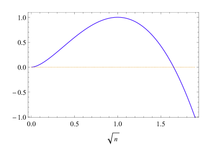
Figure 1: Field-theoretical potential density (4) of the logarithmic BEC (in units $b/{a}^{D}$) versus $|\Psi|$ (in units ${a}^{-D/2}$). Due to the normalization constraint (2), this plot must be viewed as effectively having been placed inside a well with an infinite wall starting at $n\geqslant n_{\text{cut}}$, $n_{\text{cut}}$ being some finite number.

From Fig. 1, one can easily see that the field-theoretical potential of a logarithmic BEC changes its sign when its particle density crosses a certain value, $n_{0}=\text{e}/a^{D}=\text{e}\,n_{\text{ext}}$. This switching between attraction and repulsion depending on a size can be used for explaining recent experimental data khm17 , which indicate the presence of some localization mechanism even for low-density condensates. Indeed, below we will demonstrate that this feature manifests itself in the condensate’s stability against both collapse and unbounded expansion.

In principle, one could perform a Taylor series expansion of the non-linear part $\ln(a^{D}|\Psi|^{2})$ around some point, and obtain in the lowest order the Gross-Pitaevskii equation, in the next-to-lowest order – the cubic-quintic Schrödinger equation (CQSE), and in higher orders – the higher-degree polynomial terms. All these terms describe interactions of a finite amount of particles at any given instant of time. Therefore, one might assume that the properties of the logarithmic model would be similar to those models, at least qualitatively, and the polynomial models’ properties would be able to reproduce all features of the logarithmic model by considering sufficiently many terms in the series expansion. However, this turns out to be incorrect: by restricting to any finite number of terms in series, one drastically alters the main properties of a corresponding condensate model, as we will see in the next sections. Therefore, a nonperturbative treatment is essential when dealing with the “transcendental” condensates in general and the logarithmic ones in particular.

Furthermore, the system (1) has two natural scales of length, two of time, and two of mass:

$$\text{L}=\left\{|a|,\frac{\hbar}{\sqrt{m|b|}}\right\},\ \text{T}=\left\{\frac{\hbar}{|b|},\frac{ma^{2}}{\hbar}\right\},\ \text{M}=\left\{m,\frac{\hbar^{2}}{a^{2}|b|}\right\},$$ (5)

which can be used to obtain dimensionless quantities. Assuming $a,b>0$ and

$$\vec{r}\,^{\prime}=\vec{r}/\ell,\ t^{\prime}=t/\tau,\ \psi=a^{D/2}\Psi,$$ (6)

where

$$\ell=\hbar/\sqrt{mb},\ \tau=\hbar/b,$$ (7)

we can write Eq. (1) in a dimensionless form. From Eqs. (1) and (2) we obtain, respectively:

$$i\partial_{t^{\prime}}\psi+\frac{1}{2}\Delta_{D}^{\prime}\psi+\ln(|\psi|^{2})\psi=0,$$ (8)

and

$$\left\langle\psi|\psi\right\rangle^{\prime}\equiv\int|\psi|^{2}d^{D}\vec{r}\,^{\prime}=N(a/\ell)^{D}\equiv\bar{N},$$ (9)

where $\bar{N}$ will be called the reduced number of particles.

Furthermore, the action that generates Eq. (8) can be written in a dimensionless form as

$$S[\psi,\psi^{*}]=\int\mathcal{L}^{\prime}dt^{\prime}d^{D}\vec{r}^{\prime}=\int L^{\prime}dt^{\prime},$$ (10)

where the dimensionless Lagrangian density is given by

$$\mathcal{L}^{\prime}=\frac{i}{2}(\psi\partial_{t^{\prime}}\psi^{*}-\psi^{*}\partial_{t^{\prime}}\psi)+\frac{1}{2}|\vec{\nabla}_{D}^{\prime}\psi|^{2}-|\psi|^{2}(\ln(|\psi|^{2})-1)\,,$$ (11)

and the dimensionless chemical potential $\mu^{\prime}=\mu/b$ is given as an eigenvalue of a stationary version of Eq. (8),

$$\Delta_{D}^{\prime}\phi+\left(\mu^{\prime}+4\ln{|\phi|}\right)\phi=0,$$ (12)

where $\psi(\vec{r}\,^{\prime},t^{\prime})=\exp[-i(\mu^{\prime}t^{\prime}/2)]\phi(\vec{r}\,^{\prime})$.

IV Trapless logarithmic BEC: Stability

Let us consider a spherically symmetric configuration of freely moving logarithmic BEC in a $D$-dimensional Euclidean space. For example, in a case $D=3$ this symmetry is the most natural one that can arise in absence of any trapping potentials including gravity. Note that, although a logarithmic BEC in a harmonic trap was considered in Ref. bo15 , those results cannot be directly applied to a trapless case – because in a zero trap frequency limit, the parametrization used becomes singular. Thus, for a trapless BEC, we have to start our calculations anew.

In this section, we will be omitting primes, assuming instead that length is measured in units $\ell$, time - in units $\tau$, energy - in units $b$, and so on. For the stability analysis of the logarithmic condensate we will employ the following two approaches.

IV.1 Variational approach

In order to analyze the dynamics of logarithmic condensate, it is convenient to follow a variational approach r23 ; sto97 ; r7 ; r24 ; r22 ; r28 . We will seek the solutions of Eq. (8) using the trial functions

$$\psi(r,t)=A\exp[-\frac{r^{2}}{2\xi^{2}}+i\beta r^{2}+i\alpha]\,,$$ (13)

where $A=A(t)$ is the amplitude, $\xi=\xi(t)$ is the width, $\alpha=\alpha(t)$ is the linear phase of the condensate, and $\beta=\beta(t)$ is the chirp parameter r24 ; these functions become de facto the collective degrees of freedom of the condensate. The integral over the whole space can be transformed into

$$\int d^{D}\vec{r} = \left\{\begin{array}[]{lll}\frac{2\pi^{D/2}}{\Gamma(D/2)}\int\limits_{0}^{\infty}drr^{D-1}&\text{if}&D>1,\\ \int\limits_{-\infty}^{\infty}dr&\text{if}&D=1,\end{array}\right.$$ (16)

where $\Gamma(x)$ is the Euler Gamma function. Therefore, the (reduced) number of particles (9) can be computed as

$$\bar{N}=\pi^{D/2}A^{2}\xi^{D}=\text{const},$$ (17)

whereas the averaged Lagrangian can be derived, using Eqs. (10), (11), (13) and (16), as

$$L=\pi^{D/2}A^{2}\xi^{D}\Big{[}1+\frac{D}{2}+\frac{D}{4\xi^{2}}+\frac{D}{2}\xi^{2}\left(\dot{\beta}+2\beta^{2}\right)+\dot{\alpha}-\ln A^{2}\Big{]},$$ (18)

where dot represents a time derivative. By analyzing the corresponding Euler-Lagrange equations, $\frac{\partial L}{\partial q}-\frac{d}{dt}\frac{\partial L}{\partial\dot{q}}=0$, where $q=\{A(t),\xi(t),\alpha(t),\beta(t)\}$, we obtain, after some rearrangement,

$$\dot{\alpha}+\frac{D+2}{2}\left[1+\xi^{2}\left(\dot{\beta}+2\beta^{2}\right)\right]+\frac{D-2}{4\xi^{2}}=\ln{A^{2}}\!,~{}~{}~{}$$ (19)

$$\dot{\alpha}+\frac{D}{2}\left[1+\xi^{2}\left(\dot{\beta}+2\beta^{2}\right)+\frac{1}{2\xi^{2}}\right]=\ln{A^{2}},$$ (20)

$$\dot{\xi}-2\xi\beta=0,$$ (21)

together with Eq. (17). Furthermore, these equations can be rewritten in the form

$$A^{2} = \frac{\bar{N}}{\pi^{D/2}\xi^{D}},$$ (22)

$$\alpha = \alpha_{0}+\ln{\!\left(\frac{\bar{N}}{\pi^{D/2}}\right)}\,t-\frac{D}{2}\int\left(\ln{\xi^{2}}+\frac{1}{\xi^{2}}\right)dt,~{}~{}~{}$$ (23)

$$\beta = \frac{\dot{\xi}}{2\xi},$$ (24)

and

$$\ddot{\xi}+\frac{2}{\xi}-\frac{1}{\xi^{3}}=0,$$ (25)

where $\alpha_{0}$ is an integration constant. The equations reveal that the evolution equation for width $\xi$ is a core equation of the system’s dynamics, and also that the amplitude and linear phase of the condensate are generally $D$-dependent, whereas the width and chirp do not depend on the dimensionality of the condensate.

Furthermore, for the wavefunction (13), using Eqs. (22)-(25), one can derive that

$$\left\langle r^{2}\right\rangle = \frac{1}{2}D\xi^{2},$$ (26)

$$\left\langle p^{2}\right\rangle = \frac{1}{2}\hbar^{2}D\left(\dot{\xi}^{2}+\frac{1}{\xi^{2}}\right),$$ (27)

$$\left\langle E\right\rangle = \frac{1}{2}\hbar D\left[\frac{1}{2}\dot{\xi}^{2}+\frac{1}{2\xi^{2}}+\ln{\left(\frac{\pi\xi^{2}}{\bar{N}^{2/D}}\right)}+1\right]$$ (28)

$$= \frac{1}{2\hbar}\left\langle p^{2}\right\rangle+\frac{1}{2}\hbar D\left[\ln{\left(\frac{2\pi\left\langle r^{2}\right\rangle}{D\bar{N}^{1+2/D}}\right)}+1\right]\!,~{}~{}$$

where the averages are computed using the formula

$$\langle O\rangle=\left\{\begin{array}[]{lll}\frac{2\pi^{D/2}}{\Gamma(D/2)\,\bar{N}}\int\limits_{0}^{\infty}\psi^{*}(\hat{O}\psi)\,r^{D-1}dr&\text{if}&D>1,\\ \frac{1}{\bar{N}}\int\limits_{-\infty}^{\infty}\psi^{*}(\hat{O}\psi)dr&\text{if}&D=1,\end{array}\right.$$ (29)

where $\hat{O}$ being a given operator. One can see that $\xi$ is proportional to the mean-square radius of condensate, therefore Eq. (25) can be viewed as an equation of the motion of a unit-mass fictitious particle moving in a positive $\xi$ direction

$$\ddot{\xi}=-\frac{1}{D}\frac{d}{d\xi}U(\xi),$$ (30)

where

$$U(\xi)=D\left(\frac{1}{2\xi^{2}}+\ln{\xi^{2}}\right)$$ (31)

is an effective potential, and

$${\cal E}=\frac{1}{2}\dot{\xi}^{2}+U(\xi)$$ (32)

is a fictitious particle’s energy. In terms of this mechanical analogy, the interpretation of Eq. (25) is as follows. The term proportional to $\xi^{-3}$ is related to the dispersive effect caused by a spatial gradient term in Eq. (3), while the term proportional to $\xi^{-1}$ comes from the nonlinear logarithmic term. The system’s dynamics is thus determined by competition between these terms: at small $\xi$’s the gradient term dominates, and at large $\xi$’s the logarithmic one does. From the asymptotics of Eq. (31), one can deduce that the logarithmic term should prevent the condensate from unbounded spreading ($\xi\to\infty$), whereas the gradient and logarithmic terms together should prevent the condensate from collapse ($\xi\to 0$).

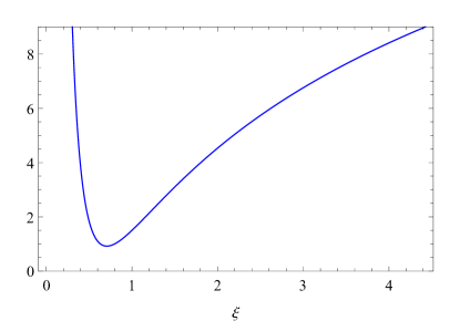
Figure 2: Effective potential (31) versus $\xi$, evaluated at $D=3$.

The potential (31) has a simple form, as shown in Fig. 2. It has a single global minimum and diverges at both small and large $\xi$’s, which means that the only allowed motion of the system is an oscillation around this minimum. The fixed-point width of the condensate can be calculated from the condition

$$\left.\frac{dU(\xi)}{d\xi}\right|_{\xi=\xi_{0}}=0,$$ (33)

which yields

$$\xi_{0}=1/\sqrt{2}.$$ (34)

Expanding Eq. (25) around this fixed pint, we obtain the dynamical equation of the width

$$\xi=\xi_{0}+A_{0}\sin(\omega_{r}t+\phi_{0})\,.$$ (35)

where $\omega_{r}$ is a frequency of collective oscillations:

$$\omega_{r}=\sqrt{\left.\frac{1}{D}\frac{d^{2}U(\xi)}{d^{2}\xi}\right|_{\xi=\xi_{0}}}=\frac{1}{\xi_{0}^{2}}\sqrt{3-2\xi_{0}^{2}},$$ (36)

and $A_{0}$ and $\phi_{0}$ are real-valued integration constants. The frequency $\omega_{r}$ can be used to analyze the stability of the condensate: the solution (34) is stable only if frequencies of collective modes are real-valued. In our case, using Eq. (34), one obtains

$$\omega_{r}=2\sqrt{2},$$ (37)

which indicates that our solution is indeed stable, without any critical points.

IV.2 Vakhitov-Kolokolov stability

Another criterion for stability is the Vakhitov-Kolokolov one vk73 , which in our case reads r24 :

$$\frac{\partial N}{\partial\mu}<0,$$ (38)

assuming our notation conventions for this section.

In order to determine the chemical potential, let us find the ground state of our system (an importance of studying the ground state’s stability is discussed in Sec. II above). One can derive that an exact ground-state solution of Eq. (12) is given by a Gaussian:

$$\phi_{0}(r)=\pm\sqrt{\bar{N}}\left(2/\pi\right)^{D/4}\exp{(-r^{2})},$$ (39)

while Eq. (12) reduces to an algebraic equation for the eigenvalue $\mu$. Solving it, we obtain

$$\mu_{0}=\ln{\left(\bar{N}_{c}^{2}/\bar{N}^{2}\right)}=\ln{\left(N_{c}^{2}/N^{2}\right)},$$ (40)

where we denoted the critical value

$$\bar{N}_{c}=N_{c}(a/\ell)^{D}=(\pi\text{e}^{2}/2)^{D/2},$$ (41)

which corresponds to the number of particles at which the chemical potential changes its sign. Using these formulae, we obtain

$$\frac{\partial N}{\partial\mu_{0}}=-\frac{1}{2}N<0,$$ (42)

which means that the trapless logarithmic condensate is also VK-stable. Moreover, its formation is energetically favorable for $N>N_{c}$.

To summarize, both approaches have shown us that the trapless $D$-dimensional logarithmic BEC is stable, even in absence of any trapping potentials, which makes it unique among all other known condensates which require external potentials for stability (cf. Sec. V). These results confirm an earlier idea r21 that the logarithmic condensate behaves more like a liquid than a gas - for instance, in the absence of any forces including gravity, it should form a Gaussian droplet which stability was demonstrated in Ref. r20 and recently confirmed by means of an orbital stability approach ard16 . The stability of such a droplet is ensured not by surface tension but by quantum nonlinear effects in its bulk.

V Trapless BEC with few-body interactions

For the sake of comparison with a logarithmic case, let us study trapless BEC with few-body interactions that evolves in the $D$-dimensional Euclidean space which is free of any external potentials including gravity. We begin by considering an isotropic BEC with both two- and three-body interactions. The formalism of Refs. r24 ; r22 ; r28 , where the $D$-dimensional condensate with two- and three-body interactions was considered in a harmonic trap, will be used in this section. However, those results alone cannot be directly applied to a completely trapless case – because in a zero trap frequency limit, some parameters used become singular. Thus, for a trapless BEC, one should start derivations anew, similar to what was done for a 3D case ackm03 ; adh04 ; svpm10 .

The wave equation for the condensate with two- and three-body interactions at zero temperature takes a form of the cubic-quintic Schrödinger equation:

$$i\hbar\frac{\partial}{\partial t}\Psi=\left[-\frac{\hbar^{2}}{2m}\Delta_{D}+\frac{\lambda_{2}}{2}|\Psi|^{2}+\frac{\lambda_{3}}{2}|\Psi|^{4}\right]\Psi,$$ (43)

where the condensate wavefunction is normalized as in Eq. (2), $\lambda_{2}$ and $\lambda_{3}$ are real coupling constants (we do not consider dissipative effects here). The corresponding Lagrangian density is given by a formula analogous to Eq. (3) where the field-theoretical potential density is defined as

$$V(n)=\frac{1}{2}\sum\limits_{k=2}^{3}\frac{\lambda_{k}}{k}n^{k}=\frac{\lambda_{2}}{4}n^{2}+\frac{\lambda_{3}}{3!}n^{3},$$ (44)

for $n=|\Psi|^{2}$.

Furthermore, because (effectively) one- and two-dimensional condensates are impossible to contain without some kind of trapping potential or geometric constraint (which is de facto a trapping potential too), we can restrict ourselves to the case

$$D>2,$$ (45)

while the lower-dimensional cases can be considered by analogy. Then the system (43) has three natural scales of length, three of time, and two of mass:

L $$= \left\{\left(\frac{m|\lambda_{2}|}{\hbar^{2}}\right)^{\frac{1}{D-2}},\left(\frac{m|\lambda_{3}|}{\hbar^{2}}\right)^{\frac{1}{2(D-1)}},\left(\frac{|\lambda_{3}|}{|\lambda_{2}|}\right)^{\frac{1}{D}}\right\},$$

T $$= \left\{\left(\frac{m^{D}\lambda_{2}^{2}}{\hbar^{D+2}}\right)^{\frac{1}{D-2}},\left(\frac{m^{D}|\lambda_{3}|}{\hbar^{D+1}}\right)^{\frac{1}{D-1}},\hbar\frac{|\lambda_{3}|}{\lambda_{2}^{2}}\right\},~{}~{}$$ (46)

M $$= \left\{m,\hbar^{2}\left(\frac{|\lambda_{3}|^{D-2}}{\lambda_{2}^{2(D-1)}}\right)^{\frac{1}{D}}\right\},$$

which can be used to obtain dimensionless quantities. Assuming $\lambda_{2}\not=0$ and introducing the notations

$$\ell_{2}=\left(\frac{m|\lambda_{2}|}{\hbar^{2}}\right)^{\frac{1}{D-2}},\ \tau_{2}=\left(\frac{m^{D}\lambda_{2}^{2}}{\hbar^{D+2}}\right)^{\frac{1}{D-2}},$$ (47)

$$\ell_{3}=\left(\frac{|\lambda_{3}|}{|\lambda_{2}|}\right)^{\frac{1}{D}},\ \tau_{3}=\hbar\frac{|\lambda_{3}|}{\lambda_{2}^{2}},$$ (48)

and

$$\vec{r}\,^{\prime}=\vec{r}/\ell_{2},\ t^{\prime}=t/\tau_{2},\ \psi=\ell_{3}^{D/2}\Psi,$$ (49)

we can write Eq. (43) in a dimensionless form:

$$i\partial_{t^{\prime}}\psi=-\frac{1}{2}\Delta_{D}^{\prime}\psi+\frac{\lambda}{2}\left(s_{2}|\psi|^{2}+s_{3}|\psi|^{4}\right)\psi,$$ (50)

where $\lambda=\tau_{2}/\tau_{3}$, and $s_{k}=\text{sgn}(\lambda_{k})=\lambda_{k}/|\lambda_{k}|$. Besides, the normalization condition reads

$$\left\langle\psi|\psi\right\rangle^{\prime}\equiv\int|\psi|^{2}d^{D}\vec{r}\,^{\prime}=N(\ell_{3}/\ell_{2})^{D}\equiv\tilde{N},$$ (51)

where $\tilde{N}$ is the reduced number of particles of the CQSE condensate. Since $\lambda$ is non-negative by construction, signs $s_{k}$ define the type of corresponding $k$-body interaction: repulsive (plus) or attractive (minus).

In this section, we do not consider the linear or orbital criteria of stability: even though nontrivial solutions of Eq. (50) do exist, they correspond to excited states of the CQSE system, therefore they will be unstable against spontaneous quantum transitions, as discussed in Sec. II. Those transitions will eventually bring the system to its ground state – which is a trivial one, $\psi_{0}=0$. In what follows, we study only the variational stability of the system, for which one does not need to know any solution of Eq. (50).

From now on, we omit primes assuming that in this section, a length is measured in units $\ell_{2}$, time - in units $\tau_{2}$, energy - in units $\hbar/\tau_{2}$, and so on. Using the formalism of Sec. IV.1, including the notations for the trial function (13), we can write the averaged Lagrangian in the form

$$L = \pi^{D/2}A^{2}\xi^{D}\Biggl{[}\frac{D}{4\xi^{2}}+\frac{D}{2}\xi^{2}\left(\dot{\beta}+2\beta^{2}\right)+\dot{\alpha}$$ (52)

$$+\frac{\lambda}{2}\left(\frac{s_{2}A^{2}}{2^{1+D/2}}+\frac{s_{3}A^{4}}{3^{1+D/2}}\right)\Biggr{]},$$

where the dot denotes a time derivative. By analyzing the corresponding Euler-Lagrange equations, we obtain

$$\dot{\beta} = \frac{\lambda\tilde{N}}{4\xi^{2}}\left(\frac{s_{2}}{(2\pi)^{D/2}\xi^{D}}+\frac{4s_{3}\tilde{N}}{\pi^{D}3^{1+D/2}\xi^{2D}}\right)$$ (53)

$$+\frac{1}{2\xi^{4}}-2\beta^{2},$$

$$\dot{\xi} = 2\xi\beta,$$ (54)

and

$$\tilde{N}=\pi^{D/2}A^{2}\xi^{D}=\text{const},$$ (55)

assuming the definition (51). From these equations one can easily derive the width equation and fictitious particle’s effective potential:

$$\ddot{\xi}=\frac{1}{\xi^{3}}+\frac{s_{2}P}{\xi^{D+1}}+\frac{s_{3}Q}{\xi^{2D+1}},$$ (56)

$$U(\xi)=\frac{D}{2\xi^{2}}+\frac{s_{2}P}{\xi^{D}}+\frac{s_{3}Q}{2\xi^{2D}},$$ (57)

where we have introduced the dimensionless magnitudes of two- and three-body interactions:

$$P=\frac{\lambda\tilde{N}}{2(2\pi)^{D/2}},\ Q=\frac{2\lambda\tilde{N}^{2}}{3^{1+D/2}\pi^{D}}=\frac{2^{1+D/2}\tilde{N}P}{3(3\pi)^{D/2}}=\frac{2^{1+D}P^{2}}{3^{1+D/2}\lambda},$$

and the fictitious particle’s energy ${\cal E}$ is given by a general formula (32).

Since we consider a case $D>2$, the potential $U(\xi)$ has the following asymptotics:

$$\xi\to 0 : \ \ U(\xi)\to\left\{\begin{array}[]{lll}s_{3}Q/(2\xi^{2D})&\text{if}&Q\not=0,\\ s_{2}P/\xi^{D}&\text{if}&Q=0,\end{array}\right.$$ (60)

$$\xi\to+\infty : \ \ U(\xi)\to 0,$$ (61)

which indicates that it always diverges in the $\xi$-origin but vanishes at spatial infinity, cf. Fig. 3. This means that, depending on values $P$, $Q$ and $s_{k}$, either $U(\xi)$ has no fixed points at $0<\xi<\infty$, or those points are extrema, hence a finite value of energy ${\cal E}$ always exists at which the fictitious particle eventually escapes to $\xi$-infinity or hits the origin $\xi=0$.

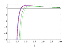
(a) $s_{2}=-1,\,s_{3}=-1$

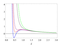
(b) $s_{2}=-1,\,s_{3}=1$

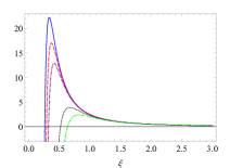
(c) $s_{2}=1,\,s_{3}=-1$

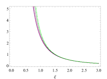
(d) $s_{2}=1,\,s_{3}=1$

Figure 3: Effective potential (57) versus $\xi$, evaluated at $D=3$, $P=1$, and different values of $Q$: $0.05$ (solid curves), $0.07$ (dashed curves), $0.1$ (dash-dotted curves), $0.5$ (dotted curves) and $1$ (dash-double-dotted curves). The upper (lower) row of panels corresponds to an attractive (repulsive) two-body interaction, while the left (right) column corresponds to an attractive (repulsive) three-body interaction.

In physical terms, this means that the trapless CQSE condensate can be, in the best case scenario, metastable: even if it is stable against the collapse ($\xi\to 0$) it is unstable against delocalization (“spreading”). The latter can be dynamic if the effective potential (57) has no local minima at $0<\xi<\infty$, cf. Figs. 3a, 3c or 3d, or spontaneous if the potential has at least one minimum at $0<\xi<\infty$, cf. the solid or dashed curve in Fig. 3b.

Within the frameworks of the variational approach, spontaneous delocalization occurs due to fluctuations of a condensate’s width $\xi(t)$, which are inevitable in the quantum realm. It can be effectively described as macroscopic tunneling of a fictitious particle towards $\xi$ infinity through a finite potential barrier, $\Delta U=U(\xi_{\text{max}})-U(\xi_{\text{min}}),$ where $0<\{\xi_{\text{max}},\,\xi_{\text{min}}\}<\infty$ are the local extrema’s points for the potential $U(\xi)$ sto97 . Note that this process should not be confused with the quantum tunneling of trapped Bose-Einstein condensates through a trap potential located in the configuration space $\vec{r}$: here we work in terms of a collective degree of freedom $\xi(t)$ and a number of particles $N$ is conserved. It should also be noted that energy ${\cal E}$ of a fictitious particle in $\xi$ space is not the same as energy of a condensate in the configuration space.

The transmission coefficient at a given energy ${\cal E}$ can be easily computed in a semiclassical approximation as

$$T({E})=\exp{\left(-2K_{23}\right)},$$ (62)

where

$$K_{jk}\equiv\int\limits_{\xi_{j}}^{\xi_{k}}\!\sqrt{2(U(\xi)-{E})}\,d\xi,$$ (63)

and $\xi_{2}$ and $\xi_{3}$ are classical turning points in a region under the barrier, $\xi_{2}<\xi_{\text{max}}<\xi_{3}$. The lifetime $\tau_{\xi}$ of the condensate which undergoes spontaneous delocalization can be easily computed in a semiclassical approximation. Assuming that the tunneling probability through the barrier $\Delta U$ is small and therefore

$$K_{23}\gg 1,$$ (64)

we obtain

$$\tau_{\xi}\approx\frac{2}{T(E)}\left(\frac{\partial J_{12}}{\partial E}\right)_{E=E_{n}},$$ (65)

where the value $E_{n}$ is a real-valued solution of the eigenvalue equation

$$J_{12}-\pi(n+1/2)=0,$$ (66)

$n$ being an integer, and

$$J_{jk}\equiv\int\limits_{\xi_{j}}^{\xi_{k}}\!\sqrt{2({E}-U(\xi))}\,d\xi,$$ (67)

and $\xi_{1}$ and $\xi_{2}$ are classical turning points in the adjacent well on the left-hand side from the barrier, $\xi_{1}<\xi_{\text{min}}<\xi_{2}<\xi_{\text{max}}<\xi_{3}$. Similarly, one can derive the characteristics of macroscopic tunneling towards the $\xi$ origin, if it is allowed by the effective potential’s form.

As a result, the trapless CQSE condensate always has a finite lifetime (except in those cases when a potential $U(\xi)$ has a global minimum at a finite positive $\xi$, with at least one negative energy ${\cal E}$ level, cf. a solid curve in Fig. 3b, and energy fluctuations are somehow suppressed): it tends to either occupy all the available volume (hence get depleted) or collapse to a state with a delta-singular density profile. In other words, it is unstable against either unrestricted expansion (hence dilution) or collapse, depending on values $P$, $Q$ and attraction/repulsion indicators $s_{k}$. Such a metastability can be easily seen in reality: models like (43) are known to be applicable for gaseous condensates, therefore, some kind of trapping potential or geometrical constraint would be necessary for their “eternal” stability, otherwise the system quickly depletes with time. As for the collapse process, in practice it stops at a length scale for which condensed atoms can no longer be regarded as point-like Bose particles, or the few-body approximation becomes no longer applicable.

Now let us consider a trapless BEC with arbitrary few-body interactions. Most of above-mentioned features remain valid – since in a minimally-coupled $U(1)$-symmetric case, such a condensate would be described by some kind of polynomially nonlinear Schrödinger equation,

$$i\hbar\frac{\partial}{\partial t}\Psi=\left[-\frac{\hbar^{2}}{2m}\Delta_{D}+\frac{1}{2}\sum\limits_{k=2}^{\cal N}\lambda_{k}|\Psi|^{2(k-1)}\right]\Psi,$$ (68)

the few-body analogue of Eqs. (56) and (57) would be, respectively:

$$\ddot{\xi}=\frac{1}{\xi^{3}}+\frac{1}{\xi}\sum\limits_{k=2}^{\cal N}\frac{I_{k}}{\xi^{(k-1)D}},$$ (69)

$$U(\xi)=\frac{D}{2\xi^{2}}+\sum\limits_{k=2}^{\cal N}\frac{I_{k}}{(k-1)\xi^{(k-1)D}},$$ (70)

where the coefficient $I_{k}=I_{k}(\lambda_{k})$ is a function of a $k$-body interaction strength parameter, $2\leqslant{\cal N}<\infty$ is a maximum amount of particles that can interact simultaneously, and the fictitious particle’s energy ${\cal E}$ is given by a general formula (32). The asymptotic properties of Eq. (70),

$$\xi\to 0 : \ \ U(\xi)\to\frac{I_{\cal N}}{({\cal N}-1)\xi^{({\cal N}-1)D}},$$ (71)

$$\xi\to+\infty : \ \ U(\xi)\to 0,$$ (72)

are qualitatively similar to Eqs. (60) and (61). As shown above, this implies, at least, the suppression of stability against unbounded expansion caused by spontaneous delocalization, due to the presence of the width’s fluctuations. This means that the trapless few-body condensates described by “polynomial” models are at best metastable, with a finite lifetime determined by Eq. (65), except in some cases when the effective potential (70) has a global minimum at $0<\xi<\infty$, with at least one negative level of energy ${\cal E}$, which can stabilize the system (in absence of energy fluctuations).

VI Conclusion

In the present work, the stability of a trapless condensate described by the logarithmic Schrödinger equation was studied and compared with a case of a trapless BEC with few-body interactions, described by wave equations with polynomial nonlinearity, such as GPE or CQSE.

By arguing that one can always expand transcendental functions, such as logarithm, into Taylor series, one might expect that the properties of the logarithmic model would be similar to the few-body models, at least qualitatively, and that the few-body models’ properties could reproduce all the features of the logarithmic model by considering sufficiently many terms in the series expansion. However, we showed that these assumptions are incorrect, in general: by restricting oneself to any finite number of terms in series, one drastically changes the main properties of a corresponding condensate model. In other words, a nonperturbative treatment is essential when dealing with the “transcendental” condensates in general and the logarithmic ones in particular.

The Gaussian variational approach and Vakhitov-Kolokolov criterion were used to determine the dynamics and stability of the logarithmic condensate, in $D$ dimensions. Using natural symmetry assumptions, we derived the collective oscillations frequency and the mean-square radius of the condensate. Further, it was demonstrated that the trapless logarithmic condensate is always stable – essentially, because logarithmic nonlinearity prevents it from both the collapse and unbounded expansion (hence dilution).

One notices that, according to Eqs. (30)-(34), trapless logarithmic Bose-Einstein condensate is attractive if its width is above a certain length scale, approximately $\xi_{0}\ell$, and repulsive if it is below. Therefore, it can be used for modeling bosenova-type phenomena when the Bose-Einstein condensate shrinks to a size smaller than the minimum resolution limit of a detector, and then rapidly expands.

Finally, stability studies of trapless condensates with few-body interactions, described by polynomially nonlinear wave equations, demonstrated that such condensates are unstable against unbounded expansion or collapse, unless one applies an external potential or geometric constraint to them. The crucial indicator here is the shape of their effective potential $U(\xi)$ which governs the dynamics of collective oscillations in terms of the width $\xi(t)$, a collective degree of freedom of a condensate. It is generally shown that: (i) if this potential has neither confining shape nor local minima then the condensate is dynamically unstable against delocalization, (ii) if this potential does not have a confining shape (e.g., it vanishes at infinity) but has at least one local minima then the condensate is metastable, i.e., unstable against the spontaneous delocalization, and thus has a finite lifetime (except in some special cases discussed below).

By comparing these features to the logarithmic case (for which the effective potential does have an absolute minimum and confining shape, cf. Fig. 2), one can deduce that “transcendental” condensates, such as the logarithmic one, can be used for describing stable quantum liquids (which was indeed shown in the work r21 ), while “polynomial” ones are a priori more suitable for describing low-density quantum matter, such as diluted cold gases (although, even there their applicability might have limits, as indicated by experiments khm17 ). Besides, a special class of trapless “polynomial” condensates exists, for which the effective potential $U(\xi)$ vanishes at infinity, has a global minimum at a finite positive $\xi$, and allows at least one negative level of effective energy ${\cal E}$. In this case, the condensate would be stable in absence of energy fluctuations (regardless of the presence of width fluctuations), but even a small increase of energy can excite the system into a metastable state with a nonzero probability of delocalization. Such models can be used for describing those condensates, which stay localized, similarly to liquids, in absence of energy fluctuations, but expand like gases otherwise.

- (1) V.E. Zakharov, Zh. Eksp. Teor. Fiz. 62, 1745 (1972) [Sov. Phys. JETP 35, 908 (1972)].
- (2) V.E. Zakharov and V.S. Synakh, Zh. Eksp. Teor. Fiz. 68, 940 (1975) [Sov. Phys. JETP 41, 465 (1975)].
- (3) M.I. Weinstein, Commun. Math. Phys. 87, 567 (1983).
- (4) L. Bergé, Phys. Rep. 303, 260 (1998).
- (5) Y. B. Gaididei et al., Phys. Rev. E 52, 2951 (1995).
- (6) H. Stoof, J. Stat. Phys. 87, 1353 (1997).
- (7) F. Dalfovo, C. Minniti, and L. P. Pitaevskii, Phys. Rev. A 56, 4855 (1997).
- (8) V. M. Pérez-García, H. Michinel, J. I. Cirac, M. Lewenstein, and P. Zoller, Phys. Rev. A 56, 1424 (1997).
- (9) L. Bergé, T. J. Alexander, and Yu. S. Kivshar, Phys. Rev. A 62, 023607 (2000).
- (10) Y. Lu, W. Xiao-Rui, L. Ke, T. Xin-Zhou, X. Hong-Wei, et al., Chin. Phys. Lett. 26, 076701 (2009).
- (11) S. E. Pollack, D. Dries, R. G. Hulet, K. M. F. Magalhẽs, E. A. L. Henn, E. R. F. Ramos, M. A. Caracanhas, and V. S. Bagnato, Phys. Rev. A 81, 053627 (2010).
- (12) A. E. Leanhardt, A. P. Chikkatur, D. Kielpinski, Y. Shin, T. L. Gustavson, et al., Phys. Rev. Lett. 89, 040401 (2002).
- (13) A. X. Zhang and J. K. Xue, Phys. Rev. A 75, 013624 (2007).
- (14) A. Gammal, T. Frederico, L. Tomio, and P. Chomaz, J. Phys. B: At. Mol. Opt. Phys. 33, 4053 (2000).
- (15) T. Köhler, Phys. Rev. Lett. 89, 210404 (2002).
- (16) N. Akhmediev, M. P. Das, and A. V. Vagov, Int. J. Mod. Phys. B 13, 625 (1999).
- (17) C. A. Jones, S. J. Putterman, and P. H. Roberts, J. Phys. A: Math. Gen. 19, 2991 (1986).
- (18) K. Watanabe, T. Mukai, and T. Mukai, Phys. Rev. A 55, 3639 (1997).
- (19) V. Efimov, Yad. Fiz. 12, 1080 (1970) [Sov. J. Nucl. Phys. 12, 589 (1971)].
- (20) V. Efimov, Phys. Lett. B 33, 563 (1970).
- (21) V. Efimov, Comments Nucl. Part. Phys. 19, 271 (1990).
- (22) W. Schöllkopf and J. P. Toennies, J. Chem. Phys. 104, 1155 (1996).
- (23) E. Nielsen, D. V. Fedorov and A. S. Jensen, J. Phys. B: At. Mol. Opt. Phys. 31, 4085 (1998).
- (24) M. A. Khamehchi, K. Hossain, M. E. Mossman, Y. Zhang, Th. Busch, M. McNeil Forbes, and P. Engels, Phys. Rev. Lett. 118, 155301 (2017).
- (25) K. G. Zloshchastiev, Grav. Cosmol. 16, 288 (2010) [arXiv:0906.4282].
- (26) K. G. Zloshchastiev, Acta Phys. Polon. B 42, 261 (2011) [arXiv: 0912.4139].
- (27) A. V. Avdeenkov and K. G. Zloshchastiev, J. Phys. B: At. Mol. Opt. Phys. 44, 195303 (2011) [arXiv:1108.0847].
- (28) K. G. Zloshchastiev, Eur. Phys. J. B 85, 273 (2012) [arXiv:1204.4652].
- (29) G. Rosen, J. Math. Phys. (N.Y.) 9, 996 (1968).
- (30) G. Rosen, Phys. Rev. 183, 1186 (1969).
- (31) I. Bialynicki-Birula and J. Mycielski, Annals Phys. 100, 62 (1976).
- (32) I. Bialynicki-Birula and J. Mycielski, Commun. Math. Phys. 44, 129 (1975);
- (33) I. Bialynicki-Birula and J. Mycielski, Phys. Scripta 20, 539 (1979).
- (34) K. G. Zloshchastiev, Phys. Lett. A 375, 2305 (2011) [arXiv:1003.0657].
- (35) V. Dzhunushaliev and K. G. Zloshchastiev, Central Eur. J. Phys. 11, 325-335 (2013) [arXiv:1204.6380].
- (36) I. E. Gulamov, E. Ya. Nugaev, and M. N. Smolyakov, Phys. Rev. D 89, 085006 (2014).
- (37) I. E. Gulamov, E. Ya. Nugaev, A. G. Panin, and M. N. Smolyakov, Phys. Rev. D 92, 045011 (2015).
- (38) V. Dzhunushaliev, A. Makhmudov, and K. G. Zloshchastiev, Phys. Rev. D 94, 096012 (2016) [arXiv:1611.02105].
- (39) H. Buljan, A. Šiber, M. Soljačić, T. Schwartz, M. Segev, and D. N. Christodoulides, Phys. Rev. E 68, 036607 (2003).
- (40) S. De Martino, M. Falanga, C. Godano, and G. Lauro, Europhys. Lett. 63, 472 (2003).
- (41) T. Hansson, D. Anderson, and M. Lisak, Phys. Rev. A 80, 033819 (2009).
- (42) E. F. Hefter, Phys. Rev. A 32, 1201 (1985).
- (43) V. G. Kartavenko, K. A. Gridnev and W. Greiner, Int. J. Mod. Phys. E 7 (1998) 287.
- (44) K. Yasue, Annals Phys. 114 (1978) 479.
- (45) N. A. Lemos, Phys. Lett. A 78 (1980) 239.
- (46) J. D. Brasher, Int. J. Theor. Phys. 30 (1991) 979.
- (47) D. Schuch, Phys. Rev. A 55, 935 (1997).
- (48) M. P. Davidson, Nuov. Cim. B 116 (2001) 1291.
- (49) J. L. Lopez, Phys. Rev. E. 69 (2004) 026110.
- (50) T. C. Scott, X. Zhang, R. B. Mann, and G. J. Fee, Phys. Rev. D 93, 084017 (2016).
- (51) W. G. Unruh, Phys. Rev. Lett. 46, 1351 (1981).
- (52) T. A. Jacobson and G. E. Volovik, Phys. Rev. D 58, 064021 (1998).
- (53) M. Visser, Class. Quant. Grav. 15, 1767 (1998).
- (54) K. G. Zloshchastiev, Acta Phys. Polon. B 30, 897-905 (1999).
- (55) G. E. Volovik, The Universe in a helium droplet, Int. Ser. Monogr. Phys. 117, 1-507 (2003).
- (56) B. Bouharia, Mod. Phys. Lett. B 29, 1450260 (2015).
- (57) D. Anderson and M. Bonnedal, Phys. Fluids 22, 105 (1979).
- (58) D.Anderson, M. Bonnedal, and M. Lisak, Phys. Fluids 22, 1839 (1979).
- (59) D. Anderson, Phys. Rev. A 27, 3135 (1983).
- (60) D. Anderson, M. Lisak and T. Reichel, J. Opt. Soc. Am. B 5, 207 (1988).
- (61) J. Fujioka and A. Espinosa, J. Phys. Soc. Japan 65, 2440 (1996).
- (62) J. Fujioka and A. Espinosa, J. Phys. Soc. Japan 82, 034007 (2013).
- (63) K. G. Zloshchastiev, Phys. Rev. B 94, 115136 (2016).
- (64) K. G. Zloshchastiev, Ann. Phys. (Berlin) 529, 1600185 (2017).
- (65) N.G. Vakhitov and A.A. Kolokolov, Izv. Vyssh. Uchebn. Zaved. Radiofiz. 16, 1020 (1973) [Radiophys. Quantum Electron. 16, 783 (1975)].
- (66) F. Kh. Abdullaev, A. Gammal, L. Tomio, and T. Frederico, Phys. Rev. A 63, 043604 (2001).
- (67) P. Ping and L. Guan-Qiang, Chin. Phys. B 18, 3221 (2009).
- (68) H. Al-Jibbouri, I. Vidanović, A. Balaž, and A. Pelster, J. Phys. B: At. Mol. Opt. Phys. 46, 065303 (2013).
- (69) A. H. Ardila, Electron. J. Diff. Equat. 2016(335), 1-9 (2016) [arXiv:1607.01479].
- (70) F. Kh. Abdullaev, J. G. Caputo, R. A. Kraenkel, and B. A. Malomed, Phys. Rev. A 67, 013605 (2003).
- (71) S. K. Adhikari, Phys. Rev. A 69, 063613 (2004).
- (72) S. Sabari, R. V. J. Raja, K. Porsezian, and P. Muruganandam, J. Phys. B: At. Mol. Opt. Phys. 43, 125302 (2010).