Disorder perturbed Flat Bands II: a search for criticality

Abstract

We present a common mathematical formulation of the level statistics of a disordered tight-binding lattice, with one or many flat bands in clean limit, in which system specific details enters through a single parameter. The formulation, applicable to both single as well as many particle flat bands, indicates the possibility of two different types of critical statistics: one in weak disorder regime (below a system specific disorder strength) and insensitive of the disorder-strength, another in strong disorder regime and occurs at specific critical disorder strengths. The single parametric dependence however relates the statistics in the two regimes (notwithstanding different scattering conditions therein). This also helps in revealing an underlying universality of the statistics in weakly disordered flat bands, shared by a wide-range of other complex systems irrespective of the origin of their complexity.

I Introduction

A dispersion-less band, also referred as a flat band, appears in crystal lattices under subtle interplay of the system conditions. The onset of disorder, say $w$ may lead to violation of these conditions, lifting the degeneracy of the energy levels and changing the nature of the eigenfunction dynamics. The important role played by these bands e.g. in magnetic systems makes it relevant to seek the detailed information about the effect of disorder on their physical properties e.g if varying disorder may lead to a localization to delocalization transition and whether its nature is similar to other disorder driven transitions.

Previous numerical studies nmg1 ; nmg2 ; cps ; lbdf on perturbed flat bands indicate the existence of two different types of transitions: an inverse Anderson transition nmg1 , independent of disorder strength, in weak disorder regime (below a system specific disorder strength, say $w_{0}$) and a standard Anderson transition in strong disorder regime mj ; emm . The different nature of these transitions originates from two types of scattering mechanism prevailing in the regimes. The wavefunction interference for $w<w_{0}$ is caused by strong back scattering due to diverging effective mass (vanishing group velocity of the wavefunction) and is insensitive to disorder strength (disorder dependent scattering being weaker) nmg1 ; nmg2 . The interference effects for $w>w_{0}$ are however due to disorder dominated scattering, resulting in a transition at a specific disorder if the band is single particle mj . In case of many particle bands, the system in $w>w_{0}$ regime undergoes a many body localization transition at one or more critical disorder strengths baa ; mg ; krav . A theoretical formulation of the transition in weak disorder regime and its connection with the one in strong disorder regime has been missing so far. Our objective here is to pursue a statistical route, analyze these transitions using spectral statistics as a tool and present an exact mathematical formulation of the transition parameter in terms of the system conditions. The later helps in identifying the universality class of the spectral statistics at each type of transition and reveal analogies if any exist.

The need to analyze the transition through statistical approach can be explained as follows. The standard search of a localization to delocalization transition, hereafter referred as LD transition, in a disordered system is based on a range of criteria e.g. the existence of an order parameter, a divergence of correlations length at the critical point, a scaling behavior for finite system sizes and critical exponents of the average physical properties. For complex systems however the fluctuation of physical properties, from one sample to another or even within one sample subjected to a perturbation, are often comparable to their average behavior and their influence on the physical properties can not be ignored. As a consequence, one has to consider criteria based on the distribution of the physical properties mj . In case of systems where the physical properties can in principle be expressed in terms of the eigenvalues and eigenfunctions of a relevant linear operator, it is appropriate to seek criteria based on their joint probability distribution function (JPDF) mj .

The definition of criticality in a JPDF of $N$ variable $x_{1},\ldots,x_{N}$ is in general based on a single parameter scaling concept mj . The distribution $P(x_{1},\ldots,x_{N};t_{1},\ldots,t_{n})$ that depends on system size $N$ and a set of $n$ parameters $t_{1},t_{2},\ldots,t_{n}$ obeys one parameter scaling if for large $N$ it is approximately a function of only variables $x_{1},..,x_{N}$ and one scale dependent parameter, say, $\Lambda\equiv\Lambda(N,t_{1},\ldots,t_{n})$. For system conditions under which the limit $\Lambda^{*}={\rm lim}_{N\rightarrow\infty}\;\Lambda(N)$ exists, the distribution approaches a universal limiting form $P^{*}(\{x\},\Lambda^{*})={\rm lim}_{N\rightarrow\infty}\;P(\{e\},\Lambda)$ and is referred as critical with $\Lambda^{*}$ as the critical parameter mj . In psf1 , we considered a typical disorder perturbed flat band, with its Hamiltonian modelled by a system-dependent ensemble of Hermitian random matrices and described a single parametric formulation of its ensemble density. As an integration of the ensemble density over all eigenfunction leads to the JPDF of its eigenvalues, this encourages us to search for a single parametric scaling of the JPDF as well as higher order eigenvalue correlations. The universal limit of these correlation, if it exists, is referred as the critical spectral statistics for the ensemble.

The concept of critical spectral statistics was first introduced in sssls in context of metal-insulator transition in disordered Hamiltonians; the study showed that the distribution $P(s)$ of the spacings $s$ between the nearest neighbor eigenvalues of the Hamiltonian turns out to be a universal hybrid of the Wigner-Dyson distribution at small-$s$ and Poisson at large-$s$, with an exponentially decaying tail: $P(s)\sim{\rm e}^{-\kappa s}$ for $s\gg 1$ with $\kappa$ as a constant sssls . The analytical studies later on indicated the criticality to manifest also through an asymptotically linear behavior of the number variance $\Sigma^{2}(r)$ (the variance in the number of levels in an spectrum interval of length $rD$) in mean number of levels $r$ with a fractional coefficient ckl .

As indicated by many studies of the transition in disordered systems, with or without particle-interactions, the wave-functions at the critical point are multifractal mj ; emm ; ms . (Note however the study gu1 claims an absence of multifractal wavefunctions in a many body systems; see pp2 in this context). This led to introduction of the singularity spectrum as the criteria for the criticality. The wave-functions in the delocalized limit are essentially structureless and overlapping almost everywhere which leads to Wigner-Dyson type level repulsion. In localized limit, the wave-functions are typically localized at different basis state with almost negligible overlap which manifests in uncorrelated level-statistics described by Poisson universality class. But the multifractality leads to an intimate conspiracy between the correlations of energy levels and eigenfunctions (for both single particle as well as many particle type). This is because the two fractal wave-functions, irrespective of their sparsity, still overlap strongly which in turn affects the decay of level correlations at long energy ranges. For $|e_{n}-e_{m}|\gg\Delta$, the correlation between two wave-functions $\psi_{n}(r)$ and $\psi_{m}(r)$ at energy $e_{n}$ and $e_{m}$ is given as ckl : $\langle|\psi_{n}(r)|^{2}|\psi_{m}(r)|^{2}\rangle\propto|e_{n}-e_{m}|^{1-(D_{2}/d)}$. In ckl , $\chi$ was suggested to be related to the multifractality of eigenfunctions too: $\chi=\frac{d-D_{2}}{2d}$ with $D_{2}$ as the fractal dimension and $d$ as the system-dimension. However numerical studies later on indicated the result to be valid only in the weak-multifractality limit emm .

Our objective in the present work is to analyze the criticality of the spectral statistics and eigenfunctions when a flat band is perturbed by the disorder. In psf1 , we analyzed the disordered tight binding Hamiltonians, with at least one flat band in the clean limit, using their matrix representation in an arbitrary basis. Presence of disorder makes it necessary to consider an ensemble of such Hamiltonians; assuming the Gaussian disorder in on-site energies (and/or interaction strengths, hopping etc) and by representing the non-random matrix elements by a limiting Gaussian, the ensemble density, say $\rho(H)$ with $H$ as the Hamiltonian, was described in psf1 by a multi-parametric Gaussian distribution, with uncorrelated or correlated matrix elements. Using the complexity parameter formulation discussed in detail in psalt ; psco ; psvalla ; psbe ; psand , the statistics of $\rho(H)$ can then be mapped to that of a single parametric Brownian ensemble (BE) appearing between Poisson and Wigner-Dyson ensemble psbe ; apbe ; fh ; me ; fkpt5 ; pslg (also equivalent to Rosenzweig-Porter model rp ). The mapping is achieved by identifying a rescaled complexity parameter of the BE with that of the disordered band. The mapping not only implies connections of the flat band statistics with the BE but also with other complex systems under similar global constraints e.g. symmetry conditions and conservation laws ps-all ; psrp . Additionally, as discussed in detail in psf1 , it also leads to a single parametric formulation of the level density and inverse participation ratio of the perturbed flat band.

In case of the BEs, the existence of a critical statistics and multifractal eigenstates is already know psbe ; krav . Their connection with disorder perturbed flat bands suggests presence of criticality in the latter too. This is indeed confirmed by our results presented here which indicate existence of a critical statistics for all weak disorders and is therefore in contrast to a single critical point in the disorder driven Anderson transition. Although the disorder independence of the statistics of a weakly disordered flat band was numerically observed in previous studies nmg2 ; viddi ; cps , its critical aspects were not explored. Another feature different from the Anderson transition is the following: with increasing disorder, the spectral statistics in a flat band undergoes a Poisson $\to$ Brownian ensemble $\to$ Poisson transition, implying a localization $\to$ extended $\to$ localization transition of the eigenstates. As well-known, the standard Anderson transition undergoes a delocalization $\to$ localization transition with increasing disorder psand . Notwithstanding these differences, the complexity parameter formulation predicts an Anderson analog of a weakly disordered flat band and also reveals its connection of to a wide range of other ensembles ps-all ; psrp ; ssps of the same global constraint class; the prediction is verified by a numerical analysis discussed later in the paper. Although the theoretical analysis presented here is based on the Gaussian disorder in flat bands but it can also be extended to other type of disorders psvalla .

The paper is organized as follows. The complexity parameter formulation for the ensemble density of a disordered tight-binding lattice, with at least one flat band in clean limit, is discussed in detail in psf1 . To avoid the repetition, we directly proceed, in section II, to review the complexity parameter formulation for the statistics of the eigenvalues and eigenfunctions. This formulation is used in sections III and IV to derive an exact mathematical expression for the transition parameter and seek criticality in the disorder perturbed flat bands; here we also analyze the influence of other neighboring bands on the statistics. A detailed numerical analysis of our theoretical claims is discussed in section V. The next section presents a numerical comparison of the spectral statistics of the disordered flat bands with two other disordered ensembles with dispersive bands, namely, the standard Anderson ensemble with on-site Gaussian disorder and Rosenzweig-Porter ensemble and confirms an analogy of their statistics for those system parameters which result in the same value of their complexity parameters. This in turn validates our theoretical claim regarding the existence of one parameter dependent universality class of statistics among disordered bands, irrespective of the underlying scattering mechanism, and more generally among complex systems subjected to similar global constraints e.g symmetry, conservation laws etc. We conclude in section VII with a brief summary of our main results.

II criticality of spectral statistics and eigenfunctions

Consider the Hamiltonian $H$ of a disorder perturbed tight binding lattice with at least one flat band in clean limit: $H=V+U$ with $V$ and $U$ as single particle and two particle interactions. By choice of a physically motivated $N$-dimensional basis, $H$ can be represented as a $N\times N$ matrix, with $N$ as a system specific parameter oh1 . Here we consider a basis, labelled by vectors $|k\rangle$, $k=1\to N$, in which (i) $H$ is Hermitian, (ii) matrix elements $H_{kl}$ are either independent or only pair-wise correlated. (For example, for $U=0$, a basis consisting of single particle states e.g. site basis can serve the purpose. Similarly, for $U\not=0$ a many body wavefunction basis mg e.g. many body Foch basis of localized single particle states or occupation number basis is appropriate oh ; see section III of psf1 for an example).

Ensemble complexity parameter: As discussed in psf1 along with a few examples, the statistical behavior of the $H$-matrix, with entries $H_{kl}$, can be modeled by a multi-parametric Gaussian ensemble if $H_{kl}$ are either independent or pairwise correlated. Assuming $e_{1},e_{2},\ldots,e_{N}$ and $U_{1},\ldots,U_{N}$ as the eigenvalues and eigenfunctions of $H$, the correlations among their various combinations can then be obtained, in principle, by an integration of the ensemble density, say $\rho(H)$, over those variables which do not appear in the combination. To study the effect of varying system conditions on the correlations, it is however easier as well as more informative to first derive an evolution equation of $\rho(H)$ which on integration leads to the evolution equations for the correlations. As described in psf1 , irrespective of the number of changing conditions, the diffusion of $\rho(H)$ undergoes a single parametric evolution

$${\partial\rho\over\partial Y} = \sum_{k,l;q}{\partial\over\partial H_{kl;q}}\left[{g_{kl}\over 2}{\partial\over\partial H_{kl;q}}+\gamma\;H_{kl;q}\;\right]\rho$$ (1)

where $g_{kl}=1+\delta_{kl}$ with $\delta_{kl}$ as a Kronecker delta function and $\gamma$ is an arbitrary constant, marking the end of the diffusion. The diffusion parameter $Y$, referred as the ensemble complexity parameter, is a combination of all ensemble parameters of $\rho(H)$ and thereby contains the information about the system parameters.

A detailed derivation of eq.(1) is technically complicated and is discussed in psco for multi parametric Gaussian ensembles (also see psalt ; ps-all ) and in psvalla for multi-parametric non-Gaussian ensembles. As an example, consider the case which can be modelled by the probability density $\rho(H,v,b)=C\;{\rm exp}[{-\sum_{q=1}^{\beta}\sum_{k\leq l}{1\over 2v_{kl;q}}(H_{kl;q}-b_{kl;q})^{2}}]$; here $q$ refers to the real ($q=1$) or imaginary ($q=2$) component of the variable, with $\beta$ as their total number, and, the variances $v_{kl;q}$ and mean values $b_{kl;q}$ can take arbitrary values (e.g. $v_{kl;q}\to 0$ for non-random cases). Using Gaussian form of $\rho(H)$, it is easy to see that a specific combination $T\rho$ of the parametric derivatives, namely, $T\rho\equiv\sum_{k\leq l;q}\left[({2\over(2-\delta_{kl})}\;x_{kl;q}\;{\partial\rho\over\partial v_{kl;q}}-\gamma\;b_{kl;q}\;{\partial\rho\over\partial b_{kl;q}}\right]$ can exactly be rewritten as the right side of eq.(1) where $x_{kl;q}\equiv 1-(2-\delta_{kl})\gamma\;v_{kl;q}$. Clearly the left side of eq.(1) must satisfy the condition $T\rho={\partial\rho\over\partial Y}$ which on solving gives $Y$ as follows psalt ; psvalla :

$$Y=-{1\over\gamma\;N_{\beta}}\;\;{\rm ln}\left[\prod_{k\leq l}\;\prod_{q=1}^{\beta}|x_{kl;q}|\quad|b_{kl;q}+b_{0}|^{2}\right]+constant$$ (2)

with $N_{\beta}={\beta N\over 2}(N+2-\beta)+N_{b}$ and $N_{b}$ as the total number of $b_{kl;q}$ which are not zero. Further $b_{0}=1$ or $0$ if $b_{kl;q}=0$ or $\not=0$ respectively. Similarly $Y$ can be formulated for the case when the matrix elements of $H$ are pairwise correlated; see psf1 and eq.(15) of psco .

Spectral density correlations: spectral complexity parameter: The statistical measures of a spectrum basically correspond to the local fluctuations of spectral density around its average value and can in principle be obtained from the $n^{th}$ order level-density correlations $R_{n}(e_{1},e_{2},..,e_{n};Y)$, defined as $R_{n}=\int\prod_{k=1}^{n}\delta(e_{k}-\lambda_{k})\;\rho(H;Y)\;{\rm D}H$. As mentioned in psf1 (see section II.C therein), eq.(1) is analogous to the Dyson’s Brownian motion model of random matrix ensembles, also referred as Brownian ensemble (see section 6.13 of fh or eq.(9.2.14) of me ). The latter describe the perturbation of a stationary Gaussian ensemble by another one with $Y$ as a perturbation parameter (or mean-square off-diagonal matrix element of the perturbation). Following exactly the same steps, as used in the derivation of eq.(6.14.21) in section 6.14 of fh , a hierarchical diffusion equation for $R_{n}$ can be derived by a direct integration of eq.(1) over $N-n$ eigenvalues and entire eigenvector space (also see section 8 of fkpt5 or apbe ; psbe ; pslg for more information). The specific case of $R_{1}(e)$ was discussed in detail in psf1 ; it varies at a scale $Y\sim N\Delta_{e}^{2}$. The solution of the diffusion equation for $R_{2}(e_{1},e_{2})$ with Poisson initial conditions is discussed in apbe (see eq.(48) therein). Contrary to $R_{1}$, $R_{n}$ with $n>1$ undergo a rapid evolution at a scale $Y\sim\Delta_{e}^{2}$, with $\Delta_{e}(e)$ as the local mean level spacing in a small energy-range around $e$. For comparison of the local spectral fluctuations around $R_{1}(e)$, therefore, a rescaling (also referred as unfolding) of the eigenvalues $e_{n}$ by local mean level spacing $\Delta_{e}(e)$ is necessary. As discussed in detail in section 6.14 of fh in context of single parametric Brownian ensembles, this leads to a rescaling of both $R_{n}$ as well as the crossover parameter $Y$, with new correlations given as ${\mathcal{R}_{n}}(r_{1},\ldots,r_{n})=\lim_{N\to\infty}\left(\Delta_{e}\right)^{n}\;R_{n}(e_{1},e_{2},..e_{n})$, where $r_{n}=e_{n}/\Delta_{e}$ and the rescaled crossover parameter $\Lambda_{e}$ given as (see eq.(6.14.12) of fh )

$$\Lambda_{e}(Y,e)={|Y-Y_{0}|\over\Delta_{e}^{2}}.$$ (3)

As discussed in psalt (see section I.E therein) and psco (see neighborhood of eq.(53) therein), eq.(3) also gives the rescaled parameter in context of multi-parametric Gaussian ensembles. (This is expected because the latter include Gaussian Brownian ensembles as a special case). As $Y$ is a combination of all ensemble parameters, $\Lambda_{e}$ can be interpreted as a measure of average complexity (or uncertainty) of the system measured in units of mean level spacing. This encourages us to refer $\Lambda_{e}$ as the spectral complexity parameter. It must be noted that $\Lambda_{e}\rightarrow\infty$ leads to a steady state i.e Gaussian orthogonal ensemble (GOE) if $H$ is real-symmetric ($\beta=1$) or Gaussian unitary ensemble (GUE) if $H$ is complex Hermitian ($\beta=2$), $\Lambda_{e}\rightarrow 0$ corresponds to an initial state psalt ; psco ; psbe . Also note that $\Delta_{e}$ here refers to the single particle mean level spacing for the single particle bands and many particle level spacing in case of the many particle bands.

In principle, all spectral fluctuation measures can be expressed in terms of ${\mathcal{R}_{n}}$; the spectral statistics as well as its criticality, therefore, depends on the system parameters and energy only through $\Lambda_{e}$. For system conditions under which the limit $\Lambda^{*}={\rm lim}_{N\rightarrow\infty}\;\Lambda_{e}(N)$ exists, ${\mathcal{R}_{n}}$ approaches a universal limiting form ${\mathcal{R}_{n}}^{*}(r_{1},\ldots,r_{n};\Lambda^{*})={\rm lim}_{N\rightarrow\infty}\;{\mathcal{R}}_{n}(r_{1},\ldots,r_{n};\Lambda_{e})$. Clearly the size-dependence of $\Lambda_{e}$ plays an important role in locating the critical point which can be explained as follows. The standard definition of a phase transition refers to infinite system sizes (i.e limit $N\to\infty$); the parameter governing the transition is therefore expected to be $N$-independent in this limit. In general, both $Y-Y_{0}$ as well as $\Delta_{e}$ and therefore $\Lambda_{e}$ can be $N$-dependent. In finite systems, a variation of $N$ therefore leads to a smooth crossover of spectral statistics between an initial state ($\Lambda_{e}\rightarrow 0$) and the equilibrium ($\Lambda_{e}\rightarrow\infty$); the intermediate statistics belongs to an infinite family of ensembles, parametrized by $\Lambda_{e}$. However, for system-conditions leading to an $N$-independent value of $\Lambda_{e}$, say $\Lambda^{*}$, the spectral statistics becomes universal for all sizes; the corresponding system conditions can then be referred as the critical conditions with $\Lambda^{*}$ as the critical value of $\Lambda_{e}$. It should be stressed that the critical criteria may not always be fulfilled by a given set of system conditions; the critical statistics therefore need not be a generic feature of all systems. (For example, it is conceivable that $\Lambda_{e}$ for a single particle flat band perturbed by disorder may not achieve size-independence at a specific energy for any disorder strength, thus indicating lack of criticality. Switching on particle-interactions however may change the size-dependence of $\Delta_{e}$ and $Y$ and lead to a size-independent $\Lambda_{e}$). This indicates an important application of the complexity parameter based formulation: $\Lambda_{e}$ provides an exact criteria, based only on a Gaussian ensemble modeling of the Hamiltonian, to seek criticality and predict presence or absence of the LD transition in a disorder perturbed flat band (single particle as well as many particles).

At the critical value $\Lambda_{e}=\Lambda^{*}$, ${\mathcal{R}}_{n}$ (for $n>1$) and therefore all spectral fluctuation measures are different from the two end points of the transition i.e $\Lambda_{e}=0$ and $\infty$ and any one of them can, in principle, be used as a criteria for the critical statistics psbe . An important aspect of these measures is their energy-dependence: ${\mathcal{R}}_{n}$ retain the dependence through $\Lambda_{e}$ even after unfolding and are non-stationary i.e vary along the spectrum psbe . Any criteria for the criticality in the spectral statistics can then be defined only locally i.e within the energy range, say $\delta e_{c}$, in which $\Lambda_{e}$ is almost constant psbe . For example, as reported by the numerical study nmg2 of diamond lattice with two flat bands, the metal insulator transition occurs only at specific energies; this energy dependence of transition can theoretically be explained using $\Lambda_{e}$ (see section IV for details).

Spectral fluctuations: standard measures: Based on previous studies, numerical as well as theoretical, two spectral measures namely nearest neighbor spacing distribution $P(s)$ and the number variance $\Sigma^{2}(r)$ are confirmed to be a reliable criteria for seeking criticality sssls ; mj ; gmp ; emm ; me in a wide range of complex systems. Here $P(s)$ measures the probability of a spacing $s$ between two nearest neighbor energy levels (rescaled by local mean level spacing) and $\Sigma^{2}(r)$ gives the variance of the number of levels in an interval of $r$ unit mean spacings. Although in past $P(s)$ has played an important role in spectral fluctuation analysis of many body systems e.g. nuclei, atoms and molecules, the numerical rescaling of a many body spectrum is subjected to technical issues e.g. exponentially increasing density of states or numerical simulation of large number of realization. This has motivated some recent studies to suggest another spectral measure for the short range correlations, namely, distribution of the level spacing ratio oh ; bog . In the present study, however, it is sufficient to consider $P(s)$ for the critical analysis; (this is because the disordered systems used in our as well as previous numerical analysis nmg2 are single particle cases with Gaussian mean level densities and the unfolding on the spectrum is easier).

As confirmed by several studies in past (see for example gmp ; mj ; emm ; me and references therein), the level fluctuations of a system in a fully delocalized wave limit behave similar to that of a Wigner-Dyson ensemble i.e GOE ($\beta=1$) for cases with time-reversal symmetry and integer angular momentum and GUE ($\beta=2$) for cases without time-reversal symmetry; here $P(s)=A_{\beta}\;s^{\beta}\;{\rm e}^{-B_{\beta}\;s^{2}}$ with $A_{1}=\pi/2,B_{1}=\pi/4,A_{2}=32/\pi^{2},B_{2}=4/\pi$ and $\Sigma^{2}(r)={2\over\pi^{2}\beta}\;\left(\ln(2\pi r)+\gamma+1+{(\beta-2)\pi^{2}\over 8}\right)$ with $\gamma=0.5772$. Similarly the fully localized case shows a behavior typical of a set of uncorrelated random levels, that is, exponential decay for $P(s)$, also referred as Poisson distribution, $P(s)={\rm e}^{-s}$, and $\Sigma^{2}(r)=r$ gmp ; mj ; me . (In case of the structured matrices e.g. those with additional constraints besides Hermiticity however Poisson spectral statistics may appear along with delocalized eigenfunctions pstp ).

For non-zero, finite $\Lambda_{e}$ cases, the exact $P(s)$ behavior is known only for the Brownian ensembles consisting of matrices of size $N=2$. As derived in ko , $P(s)$ for Poisson $\to$ GOE crossover and Poisson $\to$ GUE crossover can be given as

$$P(s,\Lambda_{e}) = \frac{s}{4\Lambda_{e}}\;{\rm exp}\left(-\frac{s^{2}}{8\Lambda_{e}}\right)\;\int_{0}^{\infty}{\rm d}x\;{\rm e}^{-{x^{2}\over 8\Lambda_{e}}-x}\;I_{0}\left(\frac{xs}{4\Lambda_{e}}\right)\hskip 72.26999pt\beta=1$$ (4)

$$P(s,\Lambda_{e}) = \frac{s}{\sqrt{2\pi\Lambda_{e}}}\;{\rm exp}\left(-\frac{s^{2}}{8\Lambda_{e}}\right)\;\int_{0}^{\infty}{\rm d}x\;{1\over x}\;{\rm e}^{-{x^{2}\over 8\Lambda_{e}}-x}\;\sinh\left(\frac{xs}{4\Lambda_{e}}\right)\hskip 36.135pt\beta=2$$ (5)

with $I_{0}$ as the modified Bessel function (see eq.(5) and eq.(11) of ko ). Here $\beta=1$ case corresponds to Brownian ensemble of real-symmetric matrices which appear as a perturbed (or non-equilibrium) state of a Poisson ensemble by a Gaussian orthogonal ensemble (also referred as the Poisson $\to$ GOE crossover) and are good models for systems with time-reversal symmetry. Similarly $\beta=2$ case corresponds to Brownian ensembles of complex Hermitian matrices, appearing as a perturbed state of a Poisson ensemble by a Gaussian unitary ensemble (also referred as Poisson $\to$ GUE crossover) and are applicable to systems without time-reversal symmetry. As $P(s)$ is dominated by the nearest neighbor pairs of the eigenvalues, this result is a good approximation also for $N\times N$ case derived in to , especially in small-$s$ and small-$\Lambda_{e}$-limit. Using the complexity parametric based mapping of the multi-parametric Gaussian ensembles of the perturbed flat bands to Brownian ensembles, the above results can directly be used for the former case too.

As mentioned above, $\Lambda_{e}$ is non-zero, finite and size-independent in the critical regime. This along with eq.(4) and eq.(5) indicates the following: $P(s)\sim{\rm e}^{-\kappa s}$, for $s\gg 1$ with $\kappa$ a constant for a finite $\Lambda_{e}$. The study sssls indicates an exponentially decaying tail of $P(s)$ as a criteria for critical spectral statistics. Similarly $\Sigma^{2}(r)$ for the critical spectral statistics is linear but with fractional coefficient: $\Sigma^{2}(r)\sim\chi\;r$ with $0<\chi<1$ mj . The coefficient $\chi$, also referred as the level compressibility, is a characteristic of the long-range correlations of levels; it is defined as, in a range $r$ around energy $e$, $\chi(e,r)=1-\int_{-r}^{r}(1-R_{2}(e,e+s))\;{\rm d}s$. As $R_{2}(e,r)$ is related to $\Sigma_{2}(e,r)$, $\chi$ can also be expressed as the $r$-rate of change of $\Sigma_{2}(e,r)$ mj ; ckl ): $\chi=\lim_{r\to\infty}{{\rm d}\Sigma^{2}(r)\over{\rm d}r}$. As discussed in psand ; psbe , $\chi$ at the critical point $\Lambda^{*}$ can be given as

$$\chi \approx 1-4\;\pi^{2}\;\Lambda^{*}\qquad{\rm small}\;\Lambda^{*}$$ (6)

$$\approx {1\over\beta\pi^{2}\Lambda^{*}}\qquad{\rm large}\;\Lambda^{*}$$ (7)

with $\chi(e,r,\Lambda=0)=1$ and $0$ for Poisson and Wigner-Dyson (GOE if $\beta=1$ or GUE if $\beta=2)$ limits, respectively. $\chi$ is also believed to be related to the exponential decay rate of $P(s)$ for large $s$: $\chi={1\over 2\kappa}$. Although $\chi$ is often used as a measure for criticality of the statistics mj but, as discussed in psbe , its numerical calculation in case of non-stationary ensembles is error-prone and unreliable.

Eigenfunction fluctuation measures: At the critical point, the fluctuations of eigenvalues are in general correlated with those of the eigenfunctions. The spectral features at the criticality are therefore expected to manifest in the eigenfunction measures too. As shown by previous studies mj ; emm , this indeed occurs through large fluctuations of their amplitudes at all length scales, and can be characterized by an infinite set of critical exponents related to the scaling of the ensemble averaged, generalized inverse participation ratio (IPR) i.e moments of the wave-function intensity with system size. At transition, ensemble average of IPR, later defined as ${\mathcal{I}}_{q}(e)=\int|\Psi({\bf r})|^{2q}\;{\rm d}{\bf r}$ for a state $\Psi({\bf r})$ with energy $e$, reveals an anomalous scaling with size $N$: $\langle{\mathcal{I}}_{q}\rangle(e)\sim N^{-(q-1)D_{q}/d}$ with $D_{q}$ as the generalized fractal dimension of the wave-function structure and $d$ as the system dimension. At critical point, $D_{q}$ is a non-trivial function of $q$, with $0<D_{q}<d$. The criticality in the eigenfunction statistics also manifests through other eigenfunction fluctuation measures e.g. IPR-distribution or two-point wave-function correlations emm . A complexity parameter based formulation for these measures is discussed in psbe ; pslg ; psf1 .

Role of dimensionality: The dimensionality dependence of the critical point in the localization $\to$ delocalization transitions of the wave-functions is well-established. This can also be seen through $\Lambda_{e}$ based formulation where dimension $d$ of the system enters mainly through local mean level spacing $\Delta_{e}(e)$ at energy $e$. This can be explained as follows. In the delocalized regime, a typical state, say $\Psi({\bf r})$ occupies the volume $L^{d}$ with $L$ as the linear size of the system which gives $|\Psi({\bf r})|^{2}={1\over L^{d}}$ (under normalization $\int_{L^{d}}|\psi({\bf r})|^{2}\;{\rm d}{\bf r}=1$). As almost all states in this regime occupy the same space with unit probability, $\Delta_{e}(e)={1\over{\langle\rho_{e}\rangle}\;L^{d}}$ with ${\langle\rho_{e}(e)\rangle}$ as the mean spectral density (i.e number of states per unit energy per unit volume): ${\langle\rho_{e}(e)\rangle}={1\over N}\langle\sum_{n=1}^{N}\delta(e-e_{n})\rangle={R_{1}\over N}$. In the localized regime, the states are typically not overlapping but localized in the same regime with a probability ${\xi^{d}\over L^{d}}$ where $\xi$ is the average localization length at energy $e$; consequently $\Delta_{e}(e)$ in this case corresponds to the level spacing in the localized volume $\xi^{d}$ and is given as $\Delta_{e}(e)={1\over\langle\rho_{e}\rangle\;\xi^{d}}={N\over R_{1}\;\xi^{d}}$. Note $\xi(e)$ is in general a function of dimensionality mj (besides other system conditions e.g. particle interactions) and can be expressed in terms of the inverse participation ratio $\overline{\langle{\mathcal{I}}_{2}\rangle}$ of the eigenfunctions in a small neighborhood of $e$ (with $\langle.\rangle$ and $\overline{.}$ implying ensemble and spectral averages respectively): $\xi^{d}=(\overline{\langle{\mathcal{I}}_{2}\rangle})^{-1}$. The above gives $\Delta_{e}(e)={N\over R_{1}}\;\overline{\langle{\mathcal{I}}_{2}\rangle}$ which on substitution in eq.(3) results in

$$\Lambda_{e}(Y,N,e)={|Y-Y_{0}|\over N^{2}}\left({R_{1}\over\overline{\langle{\mathcal{I}}_{2}\rangle}}\right)^{2}.$$ (8)

As clear from the above, a size-independence of $\Lambda_{e}(e)$ i.e existence of $\Lambda^{*}(e)$ requires a subtle cancellation of size-dependence among the ensemble complexity parameter $Y$, ensemble averaged level density $R_{1}$ and inverse participation ratio ${\mathcal{I}}_{2}$ (single particle or many particle based on the nature of the band). Note, in case of a many particle band, $\xi$ refers to many particle localization length, defined as the typical scale at which many-particle wavefunction decays and $I_{2}$ its inverse participation ratio.

In the following sections, we use eq.(8) to derive $\Lambda_{e}$ for three cases of disorder perturbed flat bands; $R_{1}$ and $I_{2}$ for these cases are derived in psf1 .

III Transition in an isolated flat band

In psf1 , we obtained the ensemble complexity parameter $Y$ for a perturbed flat band. For cases, in which disorder $w$ is the only parameter subjected to variation, $Y$ turns out to be

$$Y-Y_{0}=-{1\over N}\;{\ln|1-w^{2}|},$$ (9)

where $Y_{0}$ corresponds to the unperturbed flat band ($w=0$) and $N$ is the number of energy levels in the band.

As discussed in psf1 , the level density $R_{1}$ for an isolated flat band for arbitrary $w$ is (eq.(39) of psf1 )

$$R_{1}(e;w)={N\over\sqrt{2\pi w^{2}}}\;{\rm e}^{-{e^{2}\over 2w^{2}}}$$ (10)

Further the averaged inverse participation ratio ${\overline{\langle{\mathcal{I}}_{2}\rangle}}(e)$ for arbitrary $w$ and large $N$ can be approximated as (see section V.B of psf1 )

$${\overline{\langle{\mathcal{I}}_{2}\rangle}} \approx {6\;\pi\;u_{0}\over N\;E_{c}}\;{\rm e}^{{2\Lambda_{I}\over N}}{\rm e}^{-{4e\over E_{c}}+{e^{2}\over 2w^{2}}}$$ (11)

with $u_{0}$ as the local intensity at $e=0$ and $\Lambda_{I}={4\ln|1-w^{2}|\over E_{c}^{2}}$. Here $E_{c}$ is an energy scale associated with the range of level-repulsion around $e$ and can in general depend on $e$ as well as $w$. Eq.(11) is obtained by assuming $E_{c}\sim N^{-\mu}$ with $\mu\geq 0$ which is consistent with the definition of $E_{c}$; as discussed in psf1 , $E_{c}\sim E_{th}$ with $E_{th}$ as the Thouless energy: $E_{th}\sim o(N^{-1})$ and $o(N^{0})$ for the localized and delocalized dynamics respectively but in partially localized regime $E_{th}\sim\Delta(e).N^{D_{2}/d}$, with $\Delta(e)=(R_{1}(e))^{-1}$ as the mean level spacing at energy $e$, $D_{2}$ as the fractal dimension and $d$ as the physical dimension. Assuming $\Delta(e)\sim N^{-\eta}$ with $\eta$ as a system-dependent power, this gives

$$E_{c}\sim N^{-(\eta d-D_{2})/d}$$ (12)

and $\mu=(\eta d-D_{2})/d$. With $0\leq D_{2}\leq d$, the assumption $\mu>0$ is valid at least in flat band regime where $\eta=1$ (the latter follows from eq.(10)).

Substitution of eq.(10), eq.(11) along with eq.(9) in eq.(8) leads to

$$\Lambda_{e}(Y,N,e)={NE_{c}^{2}\over 72\;\pi^{3}\;u_{0}^{2}}\;{|\ln|1-w^{2}||\over w^{2}}\;{\rm e}^{-{16\ln|1-w^{2}|\over NE_{c}^{2}}}\;{\rm e}^{{8e\over E_{c}}-{2e^{2}\over w^{2}}}$$ (13)

As clear from the above, $\Lambda_{e}$ depends on the energy $e$, disorder $w$ as well as energy scale $E_{c}$. To seek the critical point, it is necessary to find specific $e$ and $w$ values which results in a $\Lambda_{e}$ size-independent as well as different from the two end-points: ${\lim\atop N\to\infty}\;\Lambda_{e}\not=0,\infty$. For further analysis of eq.(13), we consider following energy and disorder regimes:

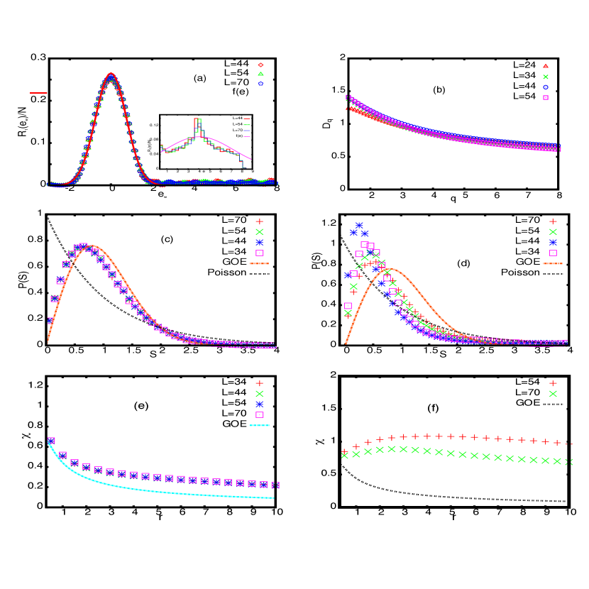
Figure 2: Critical spectral statistics for weak disorder $w=\sqrt{3}\times 10^{-5}$: (a) Level density in the flat band (inset showing the behavior in the dispersive band) with fit $f(e_{w})={1\over 2\sqrt{1.25\pi}}\;{\rm e_{w}}^{-0.8\;e_{w}^{2}}$, (b) $D_{q}$ in the flat band ($e\sim 0$), (c) $P(S)$ for flat band bulk ($e\sim 0$), (d) $P(S)$ for dispersive band bulk ($e\sim 4$), (e) $\chi(r)$ for flat band bulk ($e\sim 0$) , (f) $\chi(r)$ for dispersive band bulk ($e\sim 4$), The parts (c-e) also display the GOE and Poisson limits. Here, with $\langle{\mathcal{I}}_{2}\rangle=0.0116$ and $R_{1}\approx{0.248\;N\over w}$, eq.(23) gives $\Lambda_{e}=0.395$ near $e\sim 0$. The convergence of the curves for different sizes in parts (c, e) indicates scale-invariance of the statistics in the flat band. The behavior is critical due to $P(S)$ being different from the two end-points, namely, Poisson and GUE statistics even in large size limit. This is also confirmed by the $\chi$-behavior shown in part (e), approaching a constant value $0..2$ for large $r$, and $D_{q}$ behavior shown in part (b). Note the $\chi$-value is in agreement with eq.(7) and $D_{2}$ is consistent with relation $D_{2}=d(1-2\chi)$ with $d=2$. The survival of scale-invariance and partially localized behavior even for such a weak disorder indicates the critical point of the inverse Anderson transition to occur at zero disorder strength. In contrast, parts (d) and (f) indicate that the bulk statistics in the dispersive band is size-dependent and is not critical.

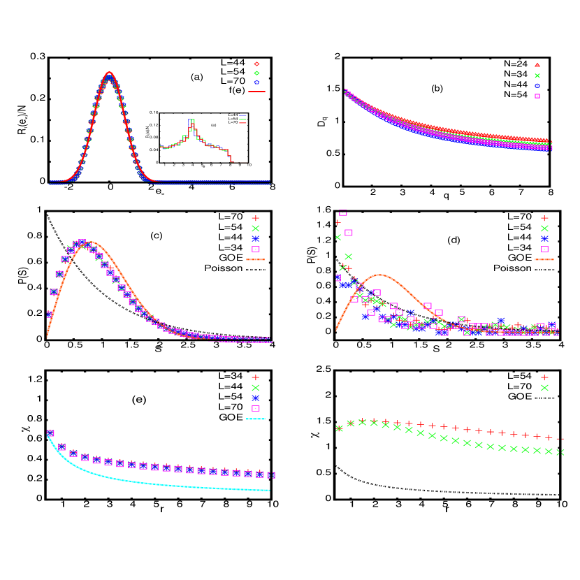
Figure 3: Critical spectral statistics for weak disorder: $w=0.1$: The details here are same as in figure 2; the fit in part (a) is $f(e_{w})={1\over 2\sqrt{1.25\pi}}\;{\rm e}^{-0.8\;e_{w}^{2}}$. Here, with $\langle{\mathcal{I}}_{2}\rangle=0.0116$ and $R_{1}(e)\approx{0.248\;N\over w}$, eq.(23) gives $\Lambda_{e}\approx 0.395$. As can be seen from parts (b) and (e) $\chi=0.2,D_{2}=1.2$ near $e\sim 0$ which is again in agreement with eq.(7) as well as relation $D_{2}=d(1-2\chi)$ with $d=2$. The analogy of the statistics with the case displayed in figure 2 indicates the disorder insensitivity of the statistics for $w<1$.

Case $e\sim 0$: For large $N$ and $E_{c}\sim N^{-\mu}$ with $0<\mu\leq 1/2$, one can approximate ${\rm e}^{-{16\ln|1-w^{2}|\over NE_{c}^{2}}}\sim 1$. This along with eq.(13) then implies disorder-independence of $\Lambda_{e}$ for $e\sqrt{2}<w<1$: $\Lambda_{e}(Y,N,e)={NE_{c}^{2}\over 72\;\pi^{3}\;u_{0}^{2}}$. Further for cases with $\mu=1/2$, $\Lambda_{e}$ is also size-independent, implying a critical spectral statistics in the bulk of the flat band spectrum (i.e $e\sim 0$). As indicated by our numerical analysis, $\eta=1,D_{2}\approx 1.18$ which gives $E_{c}\sim N^{-0.41}$ for the two dimensional chequered board lattice ($d=2$) in weak disorder limit. The criticality of the spectral statistics is also confirmed by the size-independence of the fluctuation measures (see parts (c) and (e) of the figures (2,3)). The details are discussed later in section V. (Note, for weak disorder, the chequered board lattice has a perturbed flat band in the neighborhood of a dispersive band but the former can still be treated as isolated).

For large $w$ and finite $N$, $\Lambda_{e}$ decrease smoothly with increasing $w$ and therefore the spectral statistics near $e\sim 0$ again approaches Poisson limit, implying lack of level-repulsion. Further in limit $N\to\infty$, $\Lambda_{e}\to 0$ for any finite $w>1$ which indicates a transition from critical statistics to Poisson at $w\approx 1$. As clear from the above, the statistics undergoes an inverse Anderson transition in the disorder perturbed flat band, with fully localized states at zero disorder becoming partially localized for a weak disorder ($w<1$ in our case). However the usual Anderson transition sets in presence of strong disorder ($w\simeq 1$). In infinite size limit $N\to\infty$, the statistics therefore shows two types of disorder driven critical behavior near $e\sim 0$: (i) at $w\sim 0$, Poisson $\rightarrow$ near GOE (or near GUE in presence of magnetic field) transition of the level statistics, (ii) at $w\sim 1$, the level-statistics transits from near GOE/ GUE $\rightarrow$ Poisson.

Case $e>0$: For $w^{2}<2e^{2}$, the term ${\rm e}^{-{2e^{2}\over w^{2}}}\to 0$ which gives $\Lambda_{e}\to 0$ and Poisson statistics. But, for a fixed $e>0$, ${\rm e}^{-{2e^{2}\over w^{2}}}\to 1$ with increasing $w$ and consequently $\Lambda_{e}$ increases too if $w<1$. For $w>1$, however, the contribution from other terms results in a decrease of $\Lambda_{e}$ with increasing $w$. For finite $N$ the statistics at $e>0$ therefore changes from Poisson $\to$ GOE $\to$ Poisson with increasing $w$.

An important point worth emphasizing here is an energy dependence of the spectral statistics for infinite system sizes ($N\to\infty$) and for weak disorder: critical near $e\sim 0$ if $E_{c}(e\sim 0)\propto{1\over\sqrt{N}}$ but Poisson for $e>0$ if $N\;E_{c}^{2}\leq 1$ for $e>0$. This suggests the existence of a mobility edge separating partially localized states from the localized states.

At this stage, it is relevant to indicate the following. As the level density for a flat band in clean limit can be expressed as a $\delta$-function, irrespective of whether the band is single or many particle type, the formulation derived in psf1 remains valid for both type of bands; (although $Y$ for two cases is different). Similarly the response of the average inverse participation ratio to weak disorder discussed in psf1 is based on a knowledge of initial condition only and not on the presence or absence of interactions in the band; it is thus applicable for both type of bands too. This is however not the case for the spectral fluctuations which are governed by $\Lambda_{e}$ and therefore dependent on the local mean level spacing $\Delta_{e}$. For many particle spectrum, $\Delta_{e}$ in general depends on many particle localization length which can be varied by tuning either disorder or interactions. Thus the size-independence of many body $\Delta_{e}$ can be achieved in many ways which could as a result lead to more than one critical point.

IV Transition in a flat band with other bands in the neighborhood

In presence of other bands, the energy as well as size dependence of $\Lambda_{e}$, defined in eq.(8) can vary significantly based on the neighborhood. As calculation of $\Lambda_{e}$ requires a prior knowledge of the level densities and IPR, here we consider two examples for which these measures are discussed in psf1 :

(i) two flat bands:

As discussed in section VI.A psf1 , $R_{1}(e)$ can now be expressed as a sum over two Gaussians (originating from $\delta$-function densities of two flat bands)

$$R_{1}(e;w)={N\over 2\;\sqrt{2\pi w^{2}}}\;\sum_{k=1}^{2}{\rm e}^{-{(e-e_{k})^{2}\over 2w^{2}}}$$ (14)

with $e_{1},e_{2}$ as the centers of two flat bands. The IPR in large $N$ limit is (see section VI.B of psf1 )

$${\overline{\langle{\mathcal{I}}_{2}\rangle}}(e,\Lambda_{I}) \approx {3\;u_{0}\sqrt{2\pi}\over 2\;R_{1}\;E_{c}}\;\sum_{k,l=1}^{2}{\rm e}^{-{4(e-e_{k})\over E_{c}}}\;{\rm e}^{-{(e_{l}-e_{k})^{2}\over 2w^{2}}+{2\Lambda_{I}\over N}}\;\Theta(e-e_{k})$$ (15)

with $\Lambda_{I}={4\ln|1-w^{2}|\over E_{c}^{2}}$ and $\Theta(x)$ as the step function: $\Theta(x)=0,1$ for $x<0$ and $x>0$ respectively. Substitution of eq.(14) and eq.(15) in eq.(8) now gives $\Lambda_{e}$ for this case. A better insight can however be gained by deriving $\Lambda_{e}$ in different energy regimes.

Case $e\sim e_{k}$: For $e\sim e_{k}$, with $k=1,2$, eq.(14) and eq.(15) can be approximated as $R_{1}(e;w)\approx{N\over 2\sqrt{2\pi w^{2}}}[1+{\rm e}^{-{(e_{2}-e_{1})^{2}\over 2w^{2}}}]$ and ${\overline{\langle{\mathcal{I}}_{2}\rangle}}(e)\approx{6\;\pi\;u_{0}\over N\;E_{c}}\;{\rm e}^{{8ln|1-w^{2}|\over NE_{c}^{2}}}$. These on substitution in eq.(8) give

$$\Lambda_{e}(Y,N,e)\approx{NE_{c}^{2}\over 288\;\pi^{3}\;u_{0}^{2}}\;{|\ln|1-w^{2}||\over w^{2}}\;{{\rm e}^{-{16\ln|1-w^{2}|\over NE_{c}^{2}}}\over[1+{\rm e}^{-{(e_{2}-e_{1})^{2}\over 2w^{2}}}]^{2}}$$ (16)

Clearly, similar to the single band case, here again $\Lambda_{e}$ is independent of disorder for $w<1$ and in large $N$ limit but it rapidly decreases with larger disorder (for $w>1$). Here again the size-independence of $\Lambda_{e}$ requires $E_{c}\propto{1\over\sqrt{N}}$. For $w<1$, the spectral statistics at the centers of two Gaussian bands (flat ands in clean limit) can therefore be critical as well as disorder independent only if $\mu=1/2$.

Case $e\sim(e_{1}+e_{2})/2$: For the energies midway between two bands, $R_{1}$ is very small for $w<1$ but, contrary to band center, it increases with increasing $w$ for $w>|e_{1}-e_{2}|$: $R_{1}\left({e_{1}+e_{2}\over 2}\right)={N\over\sqrt{2\pi w^{2}}}\;{\rm e}^{-{(e_{2}-e_{1})^{2}\over 8w^{2}}}$ and eq.(15) gives ${\overline{\langle{\mathcal{I}}_{2}\rangle}}(e)\approx{6\;\pi\;u_{0}\over N\;E_{c}}\;{\rm e}^{{8\;\ln|1-w^{2}|\over NE_{c}^{2}}}\;{\rm e}^{-2(e_{2}-e_{1})\over E_{c}}\;{\rm e}^{(e_{1}-e_{2})^{2}\over 8w^{2}}\;\left[1+{\rm e}^{-(e_{1}-e_{2})^{2}\over 2w^{2}}\right]$. With $Y-Y_{0}$ given by eq.(9), we now have

$$\Lambda_{e}(Y,N,e)={NE_{c}^{2}\over 72\;\pi^{3}\;u_{0}^{2}}\;{|\ln|1-w^{2}||\over w^{2}}\;{\rm e}^{-{16\;\ln|1-w^{2}|\over NE_{c}^{2}}}\;\;{{\rm e}^{4(e_{2}-e_{1})\over E_{c}}\;{\rm e}^{-(e_{1}-e_{2})^{2}\over 2w^{2}}\;\over\left(1+{\rm e}^{-(e_{1}-e_{2})^{2}\over 2w^{2}}\right)^{2}}$$ (17)

As clear from the above, here also $\Lambda_{e}$ become $N$-independent thus implying critical statistics if $E_{c}\propto N^{-1/2}$. Note however the term ${\rm e}^{-(e_{1}-e_{2})^{2}\over 2w^{2}}$ present in eq.(17) can result in the statistics different from that of $e\sim e_{k}$.

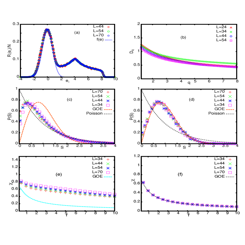
Figure 4: Critical spectral statistics for disorder: $w=1$: (a) Level density $R_{1}(e_{w})/N$ along with fit $f(e_{w})={1\over 2\sqrt{1.15\pi}}\;{\rm e}^{-0.76\;e_{w}^{2}}$ with $e_{w}=e/w$, (b) $D_{q}$ near $e\sim 0$, (c) $P(S)$ near $e\sim 0$, (d) $P(S)$ near $e\sim 4$, (e) $\chi(r)$ near $e\sim 0$, (f) $\chi(r)$ near $e\sim 4$. Here, with $\langle{\mathcal{I}}_{2}\rangle=0.0269$ and $R_{1}(e)\approx{0.261\;N\over{w}}$, eq.(23) gives $\Lambda_{e}=0.08$ near $e\sim 0$. The parts (b) and (e) now give $D_{2}=0.95,\chi=0.5$ near $e\sim 0$; this values are no longer consistent with eq.(6) or eq.(7) or relation $D_{2}=d(1-2\chi)$; the latter is however expected because the $D_{2}-\chi$ relation is expected to be valid only for small $\chi$. Further, as can be seen from part (a), the two bands start merging at this disorder strength. In contrast to weak disorder case, the statistics in flat and dispersive bands are now reversed i.e closer to Poisson and GOE respectively. But the survival of scale-invariance and partially localized behavior even for this disorder strength indicates the dominance of flat band spectrum on that of the dispersive band.

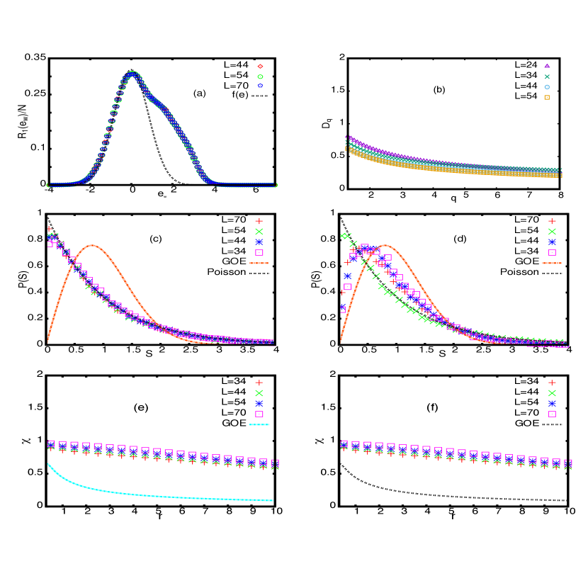
Figure 5: Critical spectral statistics for strong disorder $w=\sqrt{10}$: (a) Level density $R_{1}(e_{w})/N$ along with fit $f(e_{w})={1\over 2\sqrt{0.82\pi}}\;{\rm e}^{-1.2\;e_{w}^{2}}$ with $e_{w}=e/w$, (b) $D_{q}$ near $e\sim 0$, (c) $P(S)$ near $e\sim 0$, (d) $P(S)$ near $e\sim 4$, (e) $\chi(r)$ near $e\sim 0$, (f) $\chi(r)$ near $e\sim 4$. Here with $\langle{\mathcal{I}}_{2}\rangle=0.1149$ and $R_{1}(e)\approx 0.3\;N/{w}$, eq.(23) gives $\Lambda_{e}=1.38\times 10^{-3}$ near $e\sim 0$. As can be seen from parts (b) and (e) $\chi\approx 0.6,D_{2}=1.2$ near $e\sim 0$. Again there is no agreement with eq.(6) or relation $D_{2}=d(1-2\chi)$. Clearly eq.(6) seems to be applicable for a much smaller $\Lambda_{e}$. Further a large $D_{2}$ value here seems to be the effect of the complete merging between two bands giving rise to a new band. The statistics approaches Poisson regime and an intermediate regime for $e\sim 0$ and $e\sim 4$ respectively, both indicating localized dynamics of wave functions. The system has now reached an insulator limit in the bulk energies but is still partially localized at the edge of the new band.

A case of two flat bands was studied in nmg2 for the 3-dimensional hexagonal diamond lattice. The study indicates $D_{2}\approx 2.55$ and $2.61$ for $e\sim e_{k}$ and $e\sim(e_{1}+e_{2})/2$, respectively. With $\Delta(e)\propto N^{-1}$ and $d=3$, eq.(12) gives $E_{c}$ for this system as $N^{-0.15}$ for $e\sim e_{k}$ and $N^{-0.13}$ for $e\sim(e_{1}+e_{2})/2$. Based on our theory, the statistics is predicted to be size as well as disorder dependent near $e\sim(e_{1}+e_{2})/2$ and size-dependent but disorder-independent near $e\sim e_{k}$. The display in figures (4,5) of nmg2 indeed confirms this prediction.

The case of three flat bands was discussed in vidi , for a bipartite periodic lattice described by a tight binding, interacting Hamiltonian. The study indicates a localization $\to$ delocalization transition at the onset of disorder or many body interactions. The possibility of a critical behavior for this case can be explored along the same route as given above.

(iii) a flat band at the edge of a dispersive band: For the combination of a flat band located at $e=0$ and a dispersive band at $e>0$ with the level density $f_{d}(e)$, the results in section VI of psf1 give

$$R_{1}(e;w)={N\over 2\;\sqrt{2\pi w^{2}}}\;{\rm e}^{-{e^{2}\over 2w^{2}}}+{N\over 2}\;f_{w}(e,w,N)$$ (18)

with $f_{w}(e,w,N)$ as the dispersive band density at disorder $w$ and

$${\overline{\langle{\mathcal{I}}_{2}\rangle}}(e,\Lambda_{I}) \approx {1\over 2\;R_{1}}\;{3\sqrt{2}\over w\;E_{c}}\;\left[u_{0}\sqrt{\pi}+B_{1}+B_{2}+B_{3}\right]\;{\rm e}^{-{4e\over E_{c}}+{2\Lambda_{I}\over N}}$$ (19)

with $B_{1}={2u_{0}w\over E_{c}}\;\sqrt{\pi N\over\Lambda_{I}}\;\int_{-\infty}^{\infty}{\rm d}x\;f_{w}(x)\;{\rm e}^{-{2Nx^{2}\over\Lambda_{I}E_{c}^{2}}+{4x\over E_{c}}}$, $B_{2}=N\int_{-\infty}^{\infty}{\rm d}x\;f_{w}(x)\;u_{d}(x)\;{\rm e}^{-{x^{2}\over 2w^{2}}+{4x\over E_{c}}}$, $B_{3}={\sqrt{2\pi w^{2}}}\;\int_{-\infty}^{\infty}{\rm d}x\;f_{w}(x)\;u_{d}(x)\;{\rm e}^{4x\over E_{c}}$ and $\Lambda_{I}={4\ln|1-w^{2}|\over E_{c}^{2}}$. Here $u_{0}$ and $u_{d}(e,w)$ are the local eigenfunction intensities in the flat band at disorder $w=0$ and in dispersive band at disorder $w$. For cases in which $f_{w}(e,w,N)$ varying slower than the Gaussians in the related integrals, $B_{1}$ and $B_{2}$ can be approximated as follows: $B_{1}=\pi\sqrt{2}u_{0}\;f_{w}\left({\Lambda_{I}E_{c}\over 4}\right)\;{\rm e}^{2\Lambda_{N}\over N}$, $B_{2}=\sqrt{2\pi w^{2}}\;u_{d}\left({4w^{2}\over E_{c}^{2}}\right)\;{\rm e}^{8w^{2}\over E_{c}^{2}}$.

A substitution of eq.(18), eq.(19) along with eq.(9) in eq.(8) give $\Lambda_{e}$ for arbitrary energy and disorder but here again it is instructive to analyze the behavior near specific energies:

Case $e\sim 0$: Due to almost negligible contribution for weak disorder from the dispersive part near $e\sim 0$, one can approximate $R_{1}\approx{N\over 2\;\sqrt{2\pi w^{2}}}$ and ${\overline{\langle{\mathcal{I}}_{2}\rangle}}\approx{6{\pi}u_{0}\over NE_{c}}$ which in turn gives $\Lambda_{e}={N\;E_{c}^{2}\over 288\pi^{3}u_{0}^{2}}$. The latter is therefore again size as well as disorder independent indicating criticality near $e\sim 0$ for all weak-disorders if $E_{c}\propto N^{-1/2}$. As intuitively expected, the behavior of spectral statistics near $e\sim 0$ and $w<1$ in this case is analogous to that of the single flat band case.

As mentioned in cps ; psf1 , the two dimensional chequered board lattice consists of a flat band and a dispersive band in clean limit. Our numerical analysis of the system for $w<1$ indicated $\Delta(e)\propto N^{-1}$ and $D_{2}\sim 1.18$ (see figures 2(a,b), 3(a,b) of the present work and figure 4 of psf1 ), leading to $E_{c}\sim N^{-0.41}$ which implies ${\overline{\langle{\mathcal{I}}_{2}\rangle}}\sim N^{-0.59}$, an indicator of partially localized states pp3 . Based on theoretical grounds, therefore, the spectral statistics is expected to be critical near $e\sim 0$ and $w<1$; this is indeed confirmed by the size-independence of the statistics displayed in figure 2(c,e) and figure 3(c,e).

For large $w$ (e.g $w>1$ for the case with $\mu=1/2$), however the contribution from the dispersive band becomes significant near $e\sim 0$. This results in $R_{1}(e\sim 0)\approx{N\over 2\;\sqrt{2\pi w^{2}}}\;T_{1}$ where $T_{1}=1+\sqrt{2\pi w^{2}}\;f_{w}(0,w,N)$ and ${\overline{\langle{\mathcal{I}}_{2}\rangle}}\approx{6\;\sqrt{\pi}\over N\;E_{c}\;T_{1}}\;\left[u_{0}\sqrt{\pi}+B_{1}+B_{2}+B_{3}\right]\;{\rm e}^{{8\ln|1-w^{2}|\over NE_{c}^{2}}}$. These on substitution in eq.(8) give

$$\Lambda_{e}(Y,N,e)={NE_{c}^{2}\over 288\;\pi^{2}}\;\;{|\ln|1-w^{2}||\over w^{2}}\;{T_{1}^{4}\over\left(u_{0}\sqrt{\pi}+B_{1}+B_{2}+B_{3}\right)^{2}}\;{\rm e}^{-{16\;\ln|1-w^{2}|\over NE_{c}^{2}}}$$ (20)

As clear from the above, for large $w$ and finite $N$, $\Lambda_{e}$ decrease smoothly with increasing $w$ and therefore the spectral statistics near $e\sim 0$ again approaches Poisson limit, implying lack of level-repulsion; note $E_{c}$ is expected to decrease with increasing $w$. Further in limit $N\to\infty$, $\Lambda_{e}\to 0$ for any finite $w>1$ which indicates a transition from critical statistics to Poisson at $w\approx 1$.

The above prediction is again consistent with our numerical analysis (see figure 4(c,e) and figure 5(c,e)). Note as displayed in figure 5(a), $\Delta(e)\propto N^{-1}$ and figure 5(b), $D_{2}\approx 0.5$ which gives $E_{c}\sim N^{-0.75}$, thus implying a size-dependent $\Lambda_{e}$, approaching zero in large $N$-limit which corresponds to Poisson statistics. Figures 4(c,e) and figure 5(c,e) indeed confirm the approach of spectral measures to Poisson limit for $e\sim 0$ and $w>1$.

Case $e>0$: Due to weaker contribution from the Gaussian density for $e>0$, the contribution from the dispersive band density need not be negligible and it is appropriate to consider the full form of $R_{1}(e)$. The IPR can now be approximated as

$${\overline{\langle{\mathcal{I}}_{2}\rangle}}\approx{6\;\sqrt{\pi}\over N\;E_{c}\;T_{0}}\;\left[u_{0}\sqrt{\pi}+B_{1}+B_{2}+B_{3}\right]\;{\rm e}^{-{4e\over E_{c}}+{8\ln|1-w^{2}|\over NE_{c}^{2}}}$$ (21)

where $T_{0}={\rm e}^{-{e^{2}\over 2w^{2}}}+\sqrt{2\pi w^{2}}\;f_{w}(e)$. The above leads to

$$\Lambda_{e}(Y,N,e)={NE_{c}^{2}\over 288\;\pi^{2}}\;\;{|\ln|1-w^{2}||\over w^{2}}\;{T_{0}^{4}\over\left(u_{0}\sqrt{\pi}+B_{1}+B_{2}+B_{3}\right)^{2}}\;{\rm e}^{-{16\ln|1-w^{2}|\over NE_{c}^{2}}}\;{\rm e}^{{8e\over E_{c}}}$$ (22)

The presence of term ${\rm e}^{{8e\over E_{c}}}$ in eq.(22) results in the statistics different from the case $e\sim 0$. For $w=0$, the statistics in the dispersive band at $e>0$ is that of a GOE (or GUE if time-reversal symmetry is violated) but, with onset of disorder, it abruptly changes to Poisson. With increasing $w$ for $0<w<1$, $\Lambda_{e}$ increases but starts decreasing above $w=1$. For large $e>0$, the statistics therefore varies from GOE (at $w=0$) to Poisson statistics for $w=0^{+}$, becomes GOE at $w=1$, and then again approaches Poisson $w>1$. This prediction is consistent with our numerical results displayed in figures 2(d,f), 3(d,f) for $w<1$ and figures 4(d,f) and 5(d,f) for $w\geq 1$.

V Numerical analysis: 2-d chequered Board Lattice

To verify our theoretical predictions, we pursue a numerical statistical analysis of the eigenvalues and eigenfunctions of the Hamiltonian $H=\sum_{x,y}^{N}V_{xy}\;c_{y}^{\dagger}.c_{x}$ of a 2-$d$-planer pyrochlore lattice with single orbital per site cps ; psf1 . With 2-d unit cell labeled as $(m,n)$, one can write a site-index as $x=(m,n,\alpha)$ with $\alpha=a,b$ (i.e two atoms per unit cell). The lattice consists of one flat band $E_{f}=\varepsilon-2t$ and one dispersive band $E_{d}=\varepsilon+2t(\cos k_{x}+\cos k_{y}+1)$ if $V_{xy}$ satisfies following set of conditions psf1 ; cps : (i) $V_{xx}=\epsilon$, (ii) $V_{xy}=t$ with $x=(m,n,\alpha)$ if $y=(m,n,\beta)$ or $(m-1,n,\beta)$ or $(m,n+1,\beta)$ with $\beta=a,b$ and (iii) $V_{xy}=0$ for all other $x,y$ pairs.

For $\epsilon=2,t=1$, the Hamiltonian, in absence of disorder, consists of a flat band at $e=0$ and a dispersive band centered at $e=4$. (This can be seen from the band energies $E_{f}$ and $E_{d}$ given above). The onset of disorder through on-site energies with $\langle V_{xx}\rangle=\varepsilon,\langle V_{xx}^{2}\rangle-\langle V_{xx}\rangle^{2}=w^{2}$ leads to randomization of the Hamiltonian. For the numerical analysis, therefore, we simulate large matrix ensembles of the Hamiltonian, and at many $w$, for various ensemble-sizes $M$ (the number of matrices in the ensemble) as well as the matrix-sizes $N=L^{2}$. The energy-sensitivity of the transition (due to energy-dependence of $\Lambda_{e}$) requires the fluctuations analysis at precisely a given value of energy. In order to improve the statistics however a consideration of the averages over an optimized energy range $\Delta E$ is necessary (not too large, to avoid mixing of different statistics). For comparison of a measure for different system-sizes $N$ at a given disorder, we have used only $20\%$ levels in our numerical analysis.

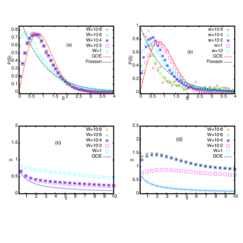
Figure 1: Disorder dependence of spectral measures in two energy ranges: (a) $P(S)$ in the bulk of flat band ($e\sim 0$), (b) $P(S)$ in the bulk of dispersive band ($e\sim 4$), (c) $\chi(r)$ in the bulk of flat band ($e\sim 0$), (d) $\chi(r)$ in the bulk of dispersive band ($e\sim 4$). Here $W=w^{2}$ and $P(S)$ refers to the distribution of the nearest-neighbor spacing $S$ and $\chi(r)$ as the spectral compressibility for the unfolded eigenvalues taken from a narrow energy-range around the specific energy for a fixed system size $L=70$. The total number of eigenvalues used in each case is approximately $10^{5}$. As clear from parts (a, c), the statistics is near GOE and disorder-insensitive for $w<1$ but approaches Poisson limit for $w>1$. Clearly, with $w=0$ as the Poisson case (due to degeneracy in flat band spectrum), increasing disorder from zero leads to a change of statistics from Poisson to near-GOE to Poisson, which corresponds to a localization-delocalization-localization crossover of the eigenfunctions in the bulk of the flat band. But parts (b,d) indicate a disorder insensitivity as well as inverse crossover in the dispersive band: with $w=0$ as GOE case, increasing disorder from zero leads to a change of statistics from GOE $\to$ Poisson $\to$ GOE which corresponds to a delocalization-localization-crossover of the eigenfunctions in the bulk of the dispersive band.

In psf1 , we theoretically analyzed the disorder dependence of level density $R_{1}$ and average inverse participation ratio $\langle I_{2}\rangle$. Our results indicated a disorder insensitivity of these measures in weak disorder limit ($w<1$). This was also confirmed by their numerical analysis as well as that of $D_{q}$ displayed in figure 4 of psf1 . A search for criticality however also requires an analysis of the size-dependence of the fluctuation measures. In this section, we numerically analyze the disorder and size dependence of the spectral fluctuations as well as the fractal dimensions $D_{q}$. The figure 1 displays the disorder-dependence of $P(s)$ and $\Sigma^{2}(r)$ in two energy regimes i.e near $e\sim 0$ and $e\sim 4$ (corresponding to bulk of the flat band and dispersive bands in clean limit). As clear from figures 1(a) and 1(c), for a weak disorder ($w<1$) and near $e\sim 0$, both measures are insensitive to change in disorder. But as displayed in figures 1(b,d), the statistics in the dispersive band ($e\sim 4$) varies with disorder even for weak disorders. A similar result was reported by the numerical study of a $3$-dimensional disordered diamond lattice (with two flat bands in the clean limit) nmg2 . The effect of on-site disorder for the ${\mathcal{T}}_{3}$ lattice with three flat bands in clean limit, was analyzed in viddi . The results again indicated disorder independence of the fluctuation measures for low disorder $w<1$ but an increase of localization with $w$ for $w>1$.

Our next step is to seek criticality in the spectral and eigenfunction statistics. For this purpose, we focus on the size-dependence of $P(S),\chi$ and $D_{2}$ in two energy regimes $e\sim 0$ and $e\sim 4$; the results for four disorder-strengths, two in weak and two in strong disorder regime, are displayed in figures 2-5. (Here, for clarity of presentation, a comparison with theoretical approximation given by eq.(4) is not displayed). To determine $\Lambda_{e}$ for these cases, it is numerically easier to use the following expression (instead of the theoretical approximation discussed in the previous section),

$$\Lambda_{e,FE}={R_{1}^{2}\over\langle I_{2}\rangle^{2}}\;{|\ln|1-w^{2}||\over N^{3}}.$$ (23)

where $R_{1}$ and $\langle I_{2}\rangle$ are numerically obtained; the corresponding values are given in the captions of figures 2-5. Before proceeding further, it is important to note that the intial condition $w=0$ (clean limit) corresponds to $\Lambda_{e}=0$ but the initial state of the statistics is different in the two bands. In clean limit, the flat band corresponds to Poisson statistics while dispersive band corresponds to that of the GOE.

The size-independence as well as location of the curves, intermediate to Poisson and GOE limits in figure 2(c,e) is an indicator of the critical spectral statistics; note the disorder here is very weak ($w\sim 10^{-5}$). Similarly behavior in figure 2(b) is an indicator of the partially localized wave-functions pp3 ; emm in the weakly disordered flat band bulk; also note that figures 2(b) and 2(e) give $D_{2}\approx 1.2$ and $\chi\approx 0.2$ respectively for the flat band which agrees well with the prediction based on the weak multifractality relation $D_{2}=d(1-2\chi)$ (note $d=2$ in our case) ckl . With $\Lambda_{e}\approx 0.384$ in this case (see caption of figure 2), the numerically obtained $\chi$-value is also consistent with eq.(7). In contrast to behavior near $e\sim 0$, the size-dependence of the measures is clearly visible from figures 2(d,f) (depicting behavior near $e\sim 4$) which rules out criticality in the dispersive regime. Furthermore the statistics here is almost Poisson which indicates an abrupt transition from GOE (for $w=0$) with onset of disorder;

As shown in figures 3(b,c,e), the critical behavior in the flat band persists even when disorder is varied to $w\sim 10^{-1}$. But in contrast to $w\sim 10^{-5}$, the statistics in the dispersive regime ($e\sim 4$) now shifts away from the Poisson limit (see figures 2(d,f) and 3(d,f)); this implies a tendency of the wave-functions in the dispersive band to increasingly delocalize as $w$ approaches $1$. The results given in figures 2 and 3 clearly indicate the reverse trend of the statistics in two bands with increasing disorder in range $0<w\leq 1$: the flat band bulk undergoes a Poisson $\to$ near GOE $\to$ near Poisson type crossover with increasing $w$ (though never reaching GOE) but the dispersive bulk changes from GOE $\to$ Poisson $\to$ GOE limit. For $w>1$ however bands increasingly overlap with each other and the statistics for both energy ranges approaches Poisson limit with increasing disorder (although at different rate based on energy regime, see figures 4,5), as expected from a standard Anderson transition (later discussed in more detail in emm ). The statistics now seems to be size-independent for all energy ranges. Also note from figures 5(b,e), the relation $D_{2}=d(1-2\chi)$ is no longer so well-satisfied near $e\sim 0$ (here $d=2$, $D_{2}\approx 0.5$ from figure 5(b) and $\chi\approx 0.42$ from figure 5(e)). This is expected because the multifractality in the band is no longer weak.

As confirmed by a large number of theoretical, numerical as well as experimental studies of wide-ranging complex systems gmp ; mj ; emm ; me , Poisson and GOE type behavior of the spectral statistics are indicators of localized and delocalized dynamics of the eigenfunctions, respectively, with an intermediate statistics indicating partially localized states pp3 ; (note, as discussed in pstp , the above relation between spectral statistics and eigenfunction dynamics is valid only for Hermitian matrices). This implies that, for $w\sim 10^{-5}$ and $10^{-1}$, the states near $e\sim 0$ are extended (although not completely delocalized) but localized near $e\sim 4$ (see parts (c),(d) of figures 2,3). For $w=1$, however the localization tendency is now reversed, with almost localized states near $e\sim 0$ but delocalized near $e\sim 4$. This inverse eigenstate localization tendency at $e\sim 0$ to the at $e\sim 4$ for a given weak disorder hints at the existence of a mobility edge/region. Note beyond $w>1$, all states are almost localized although the rate of change of localization length with disorder strength is energy-dependent (This follows because the average localization length in general depends on both disorder as well as energy).

Let us now focus on the flat band only. As clear from the above, the behavior near $e\sim 0$ indicates the occurrence of an inverse Anderson transition, with fully/ compact localized states at zero disorder becoming partially localized for a non-zero weak disorder ($w<1$ in our case). However the usual Anderson transition sets in presence of the strong disorder (for $w\geq 1$). The quantum dynamics near $e\sim 0$ now shows two types of critical behavior: (i) at $w=0$, a localized $\to$ extended state transition , in weak disorder regime and (ii) an extended state $\to$ localization transition at $w\approx 1$.

VI Analogy with other ensembles

Based on the complexity parametric formulation, different ensembles subjected to same global constraint (which is the Hermitian nature of $H$-matrix in present study) are expected to undergo similar evolution. This in turn implies an analogy of their statistical measures if the values of their complexity parameters are equal and the initial conditions are statistically analogous. In this section, we verify the analogy by comparing the statistical behavior of weakly disordered flat bands with two other disordered ensembles of real-symmetric matrices, namely, the Anderson ensemble with on-site Gaussian disorder and Rosenzweig-Porter ensemble. Similar to flat band lattices, both of these ensembles can be expressed as a multi-parametric Gaussian ensemble and the expressions for $Y$ and $\Lambda_{e}$ for them can be easily obtained (see psand , psrp and psbe for details). The two ensembles can briefly be described as follows.

Anderson Ensemble: The standard Anderson Hamiltonian $H=\sum_{k=1}^{N}\varepsilon_{k}\;c_{k}^{\dagger}.c_{k}+\sum_{k,l=n.n}^{N}V_{kl}\;c_{k}^{\dagger}.c_{l}$ describes the dynamics of an electron moving in a random potential in a $d$-dimensional tight binding lattice with one atom per unit cell. The disorder in the lattice can appear through on-site energies $\varepsilon_{k}$ or hopping $V_{kl}$ between nearest neighbor sites. Here we consider the lattice with $N$ sites, an on-site Gaussian disorder (with $\langle\varepsilon_{k}^{2}\rangle=w^{2}$, $\langle\varepsilon_{k}\rangle=0$, and a random nearest neighbor hopping ($\langle V_{kl}^{2}\rangle=t\;f_{0},\langle V_{kl}\rangle=0$ with $f_{0}=1$ if the sites $k,l$ are nearest neighbors otherwise it is zero) with $z$ as the number of nearest neighbors. The ensemble density in this case can be written as

$$\rho(H)=\lim_{\sigma\to 0}\;C_{a}\;\prod_{k=1}^{N}{\rm e}^{-{H_{kk}^{2}\over 2w^{2}}}\;\;\prod_{k,l=n.n}^{N}{\rm e}^{-{H_{kl}^{2}\over 2t}}\;\prod_{k,l\not=n.n}^{N}{\rm e}^{-{H_{kl}^{2}\over 2\sigma^{2}}}$$ (24)

with $C_{a}$ as the normalization constant. From eq.(9), the ensemble complexity parameter in this case is psand

$$Y\approx-{1\over N}\;{\rm ln}\left[|1-w^{2}|\;|1-2t|^{z/2}\right]+const,$$ (25)

Here the initial state is chosen as a clean lattice with sufficiently far off atoms resulting in zero hopping (i.e both $w=0$ and $t=0$) which corresponds to a localized eigenfunction dynamics with Poisson spectral statistics. (This choice ensures the analogy of initial statistics with the flat band case). Substitution of eq.(25) in eq.(3) with $\Delta_{e}(e)={N\langle I_{2}\rangle\over R_{1}}$ and $\overline{\langle I_{2}\rangle}$ as the typical ensemble as well as spectral averaged IPR at $e$, leads to

$$\Lambda_{e,AE}(Y,N,e)={R_{1}^{2}\over N\;\overline{\langle I_{2}\rangle}^{2}}\;{|\rm ln}(|1-w^{2}|\;|1-2t|^{z/2})|.$$ (26)

Based on the complexity parameter formulation and verified by the numerical analysis discussed in psand , the level density here turns out to be a Gaussian: $R_{1}(e)={N\over\sqrt{2\pi\alpha^{2}}}\;{\rm e}^{-{e^{2}\over 2\alpha^{2}}}$. As indicated by several studies in past (e.g mj ; emm ), the localization length $\xi$ in this case depends on the dimensionality as well as disorder: (i) $\xi\approx\pi\;l\approx O(L^{0})$ for all $w$ for $d=1$ with $l$ as the mean free path of the electron in the lattice, (ii) $\xi\approx{\rm e}^{{1\over 2}\pi lk_{F}}\approx O(L^{0})$ for all $w$ for $d=2$ with $k_{F}$ as the Fermi wave-vector and (iii) $\xi\approx\xi_{0}(e,w)\;L^{D_{2}}$ with $D_{2}={d\over 2}$ for the critical disorder $w=w^{*}$ for $d>2$. As a consequence, $\Lambda_{e}\sim O(1/N)$ for $d\leq 2$ which implies the statistics approaching an insulator limit a $N\to\infty$. For $d>2$, $\Lambda_{e}$ in the spectral bulk is size-independent only for $w=w*$ (for a fixed $t$), thus indicating only one critical point psand of transition from delocalized to localized states with increasing disorder.

An important point worth re-emphasizing is here is that notwithstanding the $N$-dependence of $Y-Y_{0}$ same for AE and the flat bands (discussed in section II.a), the statistics of energy levels and eigenfunctions in the two cases undergoes an inverse transition. This occurs because $\Lambda_{e}$, the only parameter governing the spectral statistics, depends on the localization length and mean level density which have different response to disorder $w$ in the two cases.

Rosenzweig Porter (RP) Ensemble: This represents an ensemble of Hermitian matrices with independent, Gaussian distributed matrix elements with zero mean, and different variance for the diagonals and the off diagonals. The ensemble density $\rho(H)$ in this case can be given as

$$\rho(H)\propto{\rm exp}{\left[-\frac{1}{2}\;\sum_{i=1}^{N}H_{ii}^{2}-(1+\mu_{0})\sum_{i,j=1;i<j}^{N}H_{ij}^{2}\right]}$$ (27)

As clear from the above, contrary to multi-parametric dependent Anderson case, the RP ensemble depends on the single parameter i.e ratio of the diagonal to off-diagonal variance (besides matrix size).

The ensemble density given above is analogous to the Brownian ensemble (BE) which arises due to a single parametric perturbation of an ensemble of diagonal matrices by a GOE ensemble (discussed in detail in section 2 of psand and also in psbe ). Clearly the statistics of BE or RP ensemble lies between Poisson and GOE limits and depends on a single parameter which can be given as follows. The choice of initial condition as an ensemble of diagonal matrices (which corresponds to $\mu_{0}\rightarrow\infty$) gives $Y-Y_{0}={1\over 4\mu_{0}}$ (see eq.(11) of psand , also can be seen from eq.(2) by substituting $v_{kl;q}=\delta_{kk}+{(1-\delta_{kk})\over 2(1+\mu_{0})}\delta_{q1}$, $b_{kl,q}=0$ for all $k,l$-pairs) which leads to

$$\Lambda_{e,BE}(e)=\frac{Y-Y_{0}}{\Delta_{e}(e)^{2}}=\frac{R_{1}^{2}}{4\mu_{0}}.$$ (28)

Note, the 2nd equality in the above equation is obtained by using $\Delta_{e}(e)={1\over R_{1}(e)}$ (see loc for a brief explanation).

As discussed in psbe , the size-dependence of $R_{1}(e;\mu_{0})$ for a BE or RP ensemble changes from $\sqrt{N}$ to $N$. This in turn indicates the existence of two critical points: (i) for $\mu_{0}=c_{1}N^{2}$: here $R_{1}={N\over\sqrt{\pi}}{\rm e}^{-e^{2}}$ which gives $\Lambda_{e,BE}={1\over 4\pi c_{1}}{\rm e}^{-2e^{2}}$, (ii) for $\mu_{0}=c_{2}N$: here $R_{1}(e)=(b\pi)^{-1}\;\sqrt{2bN-e^{2}}$ leading to $\Lambda(e)=\frac{2bN-e^{2}}{\pi^{2}b^{2}Nc_{2}}$ with $b\sim 2$. The two critical points here corresponds to a transition from localized $\to$ extended $\to$ delocalized states with decreasing $\mu_{0}$ psbe .

Parametric values for the analogues: For numerical analysis of Anderson ensemble, we consider a three dimensional cubic lattice with hard wall boundary conditions, on-site Gaussian disorder $w$ and a random hopping with $t=1/12$. For Brownian ensemble, we choose the case with $\mu_{0}=c\;N^{2}$; (note the latter choice is arbitrary). The system parameters for the Anderson and Brownian ensemble analogs of a weakly disordered flat band can now be obtained by invoking following condition

$$\Lambda_{e,FE}=\Lambda_{e,AE}=\Lambda_{e,BE}.$$ (29)

with $\Lambda_{e,FE}$, $\Lambda_{e,AE},\Lambda_{e,BE}$ given by eq.(23), eq.(26) and eq.(28) respectively.

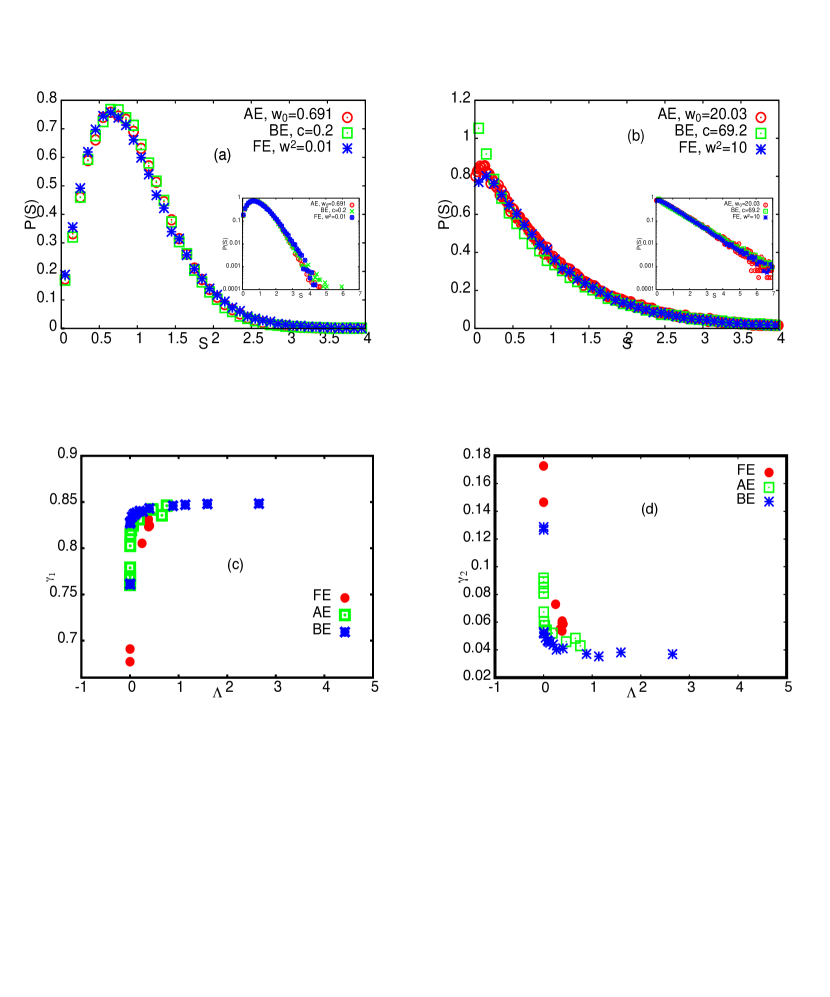
Figure 6: Comparison of Flat band ensemble (FE) with AE and BE: Here the parts (a) and (b) display the $P(s)$ comparison for the AE, BE analogues of a weakly disordered flat band for two disorders $w^{2}=0.1$ and $10$. The AE and BE analogues have been obtained by the conditions $\Lambda_{e,FE}=\Lambda_{e,AE}=\Lambda_{e,BE}$ given by eq.(23), eq.(26) and eq.(28) respectively; the system parameter for the three ensembles leading to approximately same $\Lambda_{e}$ near $e\sim 0$ are as follows: (a) FE: $N=1156,w^{2}=10^{-2},\varepsilon=2,t=1$, AE: $N=512,w^{2}={4.15\over 6},t={1\over 12}$, BE: $N=512,c=0.2$, and, (b) FE: $N=1156,w^{2}=10,\varepsilon=2,t=1$, AE: $N=512,w^{2}={120.15\over 6},t={1\over 12}$, BE: $N=512,c=69.2$. Tor rule out the accidental coincidence, we also compare $\gamma_{1}=\gamma(0.4699),\gamma_{2}=\gamma(1.9699)$ for a range of $\Lambda_{e}$ values. The results are displayed in parts (c) and (d), respectively. As clearly visible from the figures, the values for all three ensemble collapse on the same curve for small $\Lambda_{e}$ values. But while $\Lambda_{e}$ of a flat band decreases for both small and large $\Lambda_{e}$, the $\Lambda_{e}$ of an AE and BE smoothly increases from $0$ to a large value with decreasing disorder. The deviation in their behavior for large $\Lambda_{e}$ values is therefore an indicator of the different nature of transition.

Figure 6 displays a comparison of the nearest neighbor spacing distribution for two cases of disordered chequered board lattice (with Fermi energy in bulk of the flat band) with AE and BE analogues predicted by eq.(29). The numerically obtained values for the analogs near ($e\sim 0$ for each case) are as follows:

(i) weak disorder analogy: (a) FE: $N=1156$, $w^{2}=0.01$, $\varepsilon=2$, $t=1$, $\langle I_{2}^{typ}\rangle=0.0116$, $R_{1}(e)={0.248\;N\over w}$ which gives $\Lambda_{e,FE}=0.395$, (b) AE: $N=512$, $w^{2}=4.15/6$, $t=1/12$, $z=6$, $\langle I_{2}^{typ}\rangle=0.025$, $R_{1}=0.2983\times N$ with $\Lambda_{e,AE}=0.465$ and (c) BE: $N=512$, $c=0.2$ with $\Lambda_{e,BE}=0.398$.

(ii) strong disorder analogy: (a) FE: $N=1156$, $w^{2}=10$, $\varepsilon=2$, $t=1$, $\langle I_{2}^{typ}\rangle=0.1149$, $R_{1}(e)={0.3\;N\over w}$ which gives $\Lambda_{e,FE}=1.3\times 10^{-3}$, (b) AE: $N=512$, $w^{2}=120.15/6$, $\langle I_{2}^{typ}\rangle\approx 0.3$, $R_{1}\approx 0.1/N$ with $\Lambda_{e,AE}=7.58\times 10^{-4}$ and (c) BE: $N=512$, $c=69.2$ with $\Lambda_{e,BE}=1.15\times 10^{-3}$.

The AE and BE analogs for the other flat band cases can similarly be obtained. Alternatively, statistics of the perturbed flat band considered here can also be mapped to the AEs with different system conditions and the BE with $\mu_{0}\propto N$. To confirm that this analogy is not a mere coincidence and exist for other $\Lambda_{e}$ values too, we compare these ensembles for full crossover from $\Lambda_{e}=0\to\infty$. One traditionally used measure in this context is the relative behavior of the tail of nearest-neighbor spacing distribution $P(s)$, defined as

$$\gamma(\delta;\Lambda)=\frac{\int_{0}^{\delta}(P(s;\Lambda)-P(s;\infty)){\rm d}s}{\int_{0}^{\delta}(P(s;0)-P(s;\infty)){\rm d}s}$$ (30)

with $\delta$ as one of the two crossing points of $P_{o}(s)=P(s;\infty)$ and $P_{p}(s)=P(s;0)$ (here the subscripts $o$ and $p$ refer to the GOE and Poisson cases respectively) mj ; psand . As obvious, $\gamma=0$ and $1$ for GOE and Poisson limit respectively and a fractional value of $\gamma$ indicates the probability of small-spacings different from the two limits. In limit $N\to\infty$, a $\gamma$ value different from the two end points is an indicator of a new universality class of statistics and therefore a critical point. Figures 6(c) and 6(d) show a comparison of $\gamma$ for two $\delta$-values for three systems: $\gamma_{1}=\gamma(\delta_{1})$ and $\gamma_{2}=\gamma(\delta_{2})$, with $\delta_{1}=0.4699,\delta_{2}=1.9699$; the display confirms our theoretical claim regarding the analogy of the three systems. It must be noted that the $\Lambda_{e}$ for FE never approaches a value as large as that of AE and BE; following from eq.(13) and eq.(17), it first increases and then decreases beyond a disorder-strength $w\sim 1$. This is contrary to AE and BE for which $\Lambda_{e}$ decreases with increasing disorder. This behavior is also confirmed by our numerical analysis displayed in figure.

VII conclusion

In the end we summarize with main insights and results given by our analysis. We find that a disordered system, with one or more flat bands in clean limit, can undergo two types of localization to delocalization transition. In weak disorder regime (below a system specific disorder strength, say $w_{c}$), the localization is insensitive to disorder strength and persists even for a very small disorder. This in turn leads to a critical spectral statistics, disorder-independent and analogous to a Brownian ensemble intermediate to Poisson and Wigner-Dyson classes. But in strong disorder regime ($w>w_{c}$), the behavior is analogous to that of a disorder-driven, standard Anderson transition (for single particle bands) or many body localization transition (for many particle bands) in which a size-invariant spectral statistics occurs only at specific disorder strengths; the statistics here is again analogous to a Brownian ensemble but characterized by a different parameter value. The clearly reveals the influence the underlying scattering has on the transitions in the two regimes: although it affects the transition parameter dependence on disorder, the spectral statistics in both regimes belongs to one parameter dependent universality class of Brownian ensembles.

The analysis presented here is based on a single parameter formulation of the spectral statistics. This not only helps in theoretical understanding of the numerical results given by our as well as previous studies nmg2 but also reveals new features. For example, it provides a unified formulation of the spectral statistics in the weak and strong disorder regimes (notwithstanding different scattering conditions). It also identifies the spectral complexity parameter as the transition parameter and leads to its exact mathematical expression which in turn helps in the search of criticality in a disorder perturbed flat band; this occurs when the system conditions conspire collectively to render the spectral complexity parameter size-independent. More clearly, the criticality requires the ensemble complexity parameter, an indicator of the average uncertainty in the system, measured in the units of local mean level spacing, to become scale-free. The underlying localization dynamics clearly leaves its fingerprints on the transition parameter; the latter turns out to be disorder independent in weak disorder regime but is disorder dependent in strong disorder regime.

The advantage of complexity parameter based analysis goes beyond a search for criticality in perturbed flat bands. It also reveals an important analogy in the localization to delocalization crossover in finite systems: notwithstanding the difference in the number of critical points as well as equilibrium limits, the statistics of a disordered flat band can be mapped to that of a single parametric Brownian ensemble psbe as well as multi-parametric Anderson ensemble psand (see section VI). The analogy of these ensembles to other multi-parametric ensembles intermediate between Poisson and Wigner-Dyson is already known ssps ; ps-all ; psvalla ; psbe . In fact it seems a wide range of localization $\to$ delocalization transition can be modeled by a single parameter Brownian ensemble appearing between Poisson and GOE (Rosenzweig-Porter ensemble) psrp . This hints at a large scale universality and a hidden web of connection underlying complex systems even for partially localized regime. Note the universality of spectral statistics and eigenfunctions in ergodic or delocalized waves regime is already known but the complexity parameter formulation reveals a universality even at the critical point of widely different systems (of same global constraint class) if their complexity Parameters are equal. It is relevant for the following reason: it is well known that average properties of systems often show a power law behavior at the critical point and can be classified into various universality classes based on their powers, referred as the critical exponents. However, in case of a complex system where the fluctuations of physical properties are often comparable to their averages, it is not enough to know the universality classes of critical exponents. An important question in this context is whether there are universality classes among the fluctuation properties too? As discussed in section VI, such universality classes can indeed be identified based on the complexity parameter formulation. This issue will be discussed in more detail in a future publication.

Our study gives rise to many new queries. For example, an important question is whether weak particle-particle interactions in clean flat bands can mimic the role of weak disorder in the perturbed flat bands. At least the complexity parameter formulation predicts this to be the case but a thorough investigation of the fluctuations is needed to confirm the prediction. A detailed analysis of the role of the symmetries in flat band physics using complexity parameter approach still remains to be investigated. Our analysis seems to suggest the existence of a mobility edge too however this requires a more thorough investigation. We expect to explore some of these questions in future.

References

- (1) M. Goda, S. Nishino and H. Matsuda, Phys. Rev. Lett. 96, 126401, (2006).
- (2) S. Nishino, H. Matsuda and M. Goda, J. Phys. Soc. of Japan, 76, 024709, (2007);
- (3) J.T. Chalker, T.S. Pickles and P. Shukla, Phys. Rev. B, 82, 104209, (2010).
- (4) D. Leykam, J.D.Bodyfelt, A.D.Desyatnikov and S. Flach, Eur. Phys. J. B, 90, 1, (2017).
- (5) M. Janssen, Phys. Rep. 295, 1, (1998).
- (6) A.D. Mirlin and F. Evers, Rev. Mod. Phys. 80, 1355, (2008). F. Evers, A. Mildenberger and A.D. Mirlin, Phys. Rev. B 64, 241303, (2001).
- (7) D. Basko, I. Aleiner, and B. Altshuler, Ann. Phys. 321, 1126 (2006).
- (8) C. Monthus and T. Garel, Phys. Rev. B 81, 134202, (2010).
- (9) V.E. Kravtsov, I.M. Khaymovich, E.Cuevas and M. Amini, New. J. Phys (IOP), (2016).
- (10) B.I. Shklovskii, B. Shapiro, B.R.Sears, P. Lambrianides and H.B.Shore, Phys. Rev. B 47, 11487, (1993).
- (11) J.T.Chalker, V.E.Kravtsov and I.V.Lerner, Pis’ma Zh. Eksp. Teor. Fiz. 64, 355 (1996) [JETP Lett. 64, 386, (1996)].
- (12) Maksym Serbyn, Z. Papić, and Dmitry A. Abanin, Phys. Rev. B 96, 104201, (2017); M. Pino, V. E. Kravtsov, B. L. Altshuler, and L. B. Ioffe Phys. Rev. B 96, 214205, (2017); X. Chen, X. Yu, G.Y.Cho, B.K.Clark, and E. Fradkin Phys. Rev. B 92, 214204, (2015); D. J. Luitz, F. Alet, and N. Laflorencie, Phys. Rev. Lett. 112, 057203, (2014); J. Lindinger and A. Rodríguez, Acta Physica Polonica A, 132, 1683, (2017).
- (13) Z. Gulacsi, Phys. Rev. B 69, 054204, (2004)); Z. Gulacsi, A. Kampf and D. Vollhardt, Phys. Rev. Lett., 99, 026404, (2007).
- (14) The matrix representation of an operator depend on the choice of the basis and the constraints on the dynamics. This in turn also affects the behavior of the eigenfunctions (due to their basis-dependence). Previous studies claiming multifractal eigenfunctions at a critical point are often concerned with Hamiltonian matrices with Hermiticity as the only constraint. For cases where the system is subjected to additional constraints e.g.those resuling in positive semidefinite matrices as in gu1 , further investigations are needed to confirm the mutifractality.
- (15) P. Shukla, Phys. Rev. B, 98, 054206, (2018).
- (16) P.Shukla, Phys. Rev. E 62, 2098, (2000).
- (17) P.Shukla, Phys. Rev. E, 71, 026266, (2005).
- (18) P.Shukla, J.Phys. A, 41, 304023, (2008).
- (19) P.Shukla, J. Phys.: Condens. Matter 17, 1653, (2005).
- (20) S. Sadhukhan and P. Shukla, Phys. Rev. E, 96, 012109, (2017).
- (21) F. Haake, Quantum Signatures of Chaos, (1991).
- (22) M.L.Mehta, Random Matrices, (2nd ed., Academic Press, N.Y., 1991).
- (23) J.B.French, V.K.B.Kota, A. Pandey and S. Tomsovic, Annals of Physics, 181, 198, (1988).
- (24) A. Pandey, Chaos, Solitons, Fractals, 5, 1275, (1995).
- (25) P. Shukla, J. Phys. A, 50, 435003, (2017); Phys. Rev. E, 75, 051113, (2007).
- (26) N. Rosenzweig and C.E.Porter, Phys. Rev. 120, 1698 (1960).
- (27) R. Dutta and P. Shukla, Phys. Rev. E,76, 051124, (2007). R. Dutta and P.Shukla, Phys. Rev. E 78, 031115 (2008). M V Berry and P. Shukla, J. Phys. A, 42, 485102, (2009).
- (28) P. Shukla, New J. Phys, 18, 021004, (2016).
- (29) T. Guhr, A. Muller-Groeling. And H. Weidenmuller, Phys.Rep., 299, 189, (1998).
- (30) V. Oganesyan and D.A.Huse, Phys. Rev. B 75, 155111, (2007).
- (31) The formulation presented here is applicable for an arbitray basis as long as the matrix remains Hermitian. However the choice of a basis which preseves global constraints of the system i.e the symmetry and conservation laws can provide physically relevant information; for example, it permits a comparison of different complex systems (those with same global constraints) and reveals their statistical analogies through complexity parameter formulation.
- (32) Y. Y. Atas, E. Bogomolny, O. Giraud and G. Roux, Phys. Rev. Lett. 110 084101, (2013); Y Y Atas, E Bogomolny, O Giraud, P Vivo and E Vivo, J. Phys. A: Math. Theor. 46, 355204, (2013).
- (33) J. Vidal, P. Butaud, B. Doucot, and R. Mosseri, Phys. Rev. B 64, 155306 (2001); J. Vidal, G. Monatambaux and B. Doucot, Phys. Rev. B 62, R16294, (2000).
- (34) J. Vidal, R. Mosseri and B. Doucot, Phys. Rev. Lett. 81, 5888, (1998).
- (35) J. Vidal, B. Doucot, R. Mosseri and P. Butaud, Phys. Rev. Lett. 85, 3906, (2000).
- (36) Z. Gulacsi, A. Kampf and D. Vollhardt, Phys. Rev. Lett., 105, 266403, (2010).
- (37) T. Mondal, S. Sadhukhan, P. Shukla, Phys. Rev. E, 2017; T. Mondal and P. Shukla, arXiv preprint arXiv:1807.04173.
- (38) The term “partially localized state” here refers to an eigenstate of the system which extends upto a few basis states only, say , with in a -dimensional basis. It can then be characterized by an inverse participation ratio between zero and . A fully localized state with this definition corresponds to the one confined to a single basis state and has . Similarly a delocalized state corresponds to the one extended over all basis states and has .
- (39) P. Shukla and S. Sadhukhan, J.Phys.A, 48, 415002, (2015); S. Sadhukhan and P. Shukla, J. Phys. A, 415003, (2015).
- (40) V.K.B.Kota and S.Sumedha, Phys. Rev. E, 60, 3405, (1999); E. Caurier, B. Grammaticos and A. Ramani, J. Phys. A 23, 4903, (1990); G.Lenz and F.Haake, Phys. Rev. Lett. 67, 1, (1991)
- (41) S.Tomsovic, Ph.D Thesis, University of Rochester (1986); (unpublished). F. Leyvraz and T.H.Seligman, J. Phys. A 23, 1555 (1990).
- (42) The relation is applicable only for the sparse matrices and not in case of the dense matrices. This can be explained as follows. Consider the matrix representation of an operator in an arbitrary basis , in which all off-diagonals are of the same order (as in case of a BE). The matrix element, say, can be written as with as the component of the eigenfunction corresponding to the eigenvalue of . For cases where is a random matrix, are random variables too. Clearly, for to be of the same order for all basis pairs for arbitrary , the correlation should typically be of the same order (i.e almost independent of although it may depend on ). This requires a state to typically have almost same overlap with all basis states, thus implying an extended state in the volume which in turn leads to .