Abstract

In this work, we apply a semi-Lagrangian spectral method for the Vlasov-Poisson system, previously designed for periodic Fourier discretizations, by implementing Legendre polynomials and Hermite functions in the approximation of the distribution function with respect to the velocity variable. We discuss second-order accurate-in-time schemes, obtained by coupling spectral techniques in the space-velocity domain with a BDF time-stepping scheme. The resulting method possesses good conservation properties, which have been assessed by a series of numerical tests conducted on the standard two-stream instability benchmark problem. In the Hermite case, we also investigate the numerical behavior in dependence of a scaling parameter in the Gaussian weight. Confirming previous results from the literature, our experiments for different representative values of this parameter, indicate that a proper choice may significantly impact on accuracy, thus suggesting that suitable strategies should be developed to automatically update the parameter during the time-advancing procedure.

1 Introduction

A semi-Lagrangian spectral method has been proposed in [25] for the numerical approximation of the nonrelativistic Vlasov-Poisson equations. These equations describe the dynamics of a collisionless plasma of charged particles, under the effect of a self-consistent electrostatic field [11]. For the exposition’s sake, we assume that each plasma species (electrons and ions) is described by a 1D-1V distribution function, i.e., a function defined in a phase space that is one-dimensional in the independent variables $x$ (space) and $v$ (velocity). The approximation introduced in [25] has been specifically tested on Fourier-Fourier periodic discretizations for both variables in the phase space. The main goal of this paper is to extend our approach to Fourier-Legendre and Fourier-Hermite discretizations, i.e., by considering the spectral type representation with respect to $v$ provided by Hermite and Legendre polynomials, in conjunction with a high-order semi-Lagrangian technique in time.

Semi-Lagrangian methods have been proposed in different frameworks such as the Finite Volume method [26, 4], Discontinuous Galerkin method [2, 3, 39], finite difference methods based on ENO and WENO polynomial reconstructions [21], as well as in the propagation of solutions along the characteristics in an operator splitting context [1, 17, 20, 28, 27, 52, 23]. These methods offer an alternative to Particle-in-Cell (PIC) methods [22, 58, 59, 12, 18, 19, 42, 43, 47, 53] and to the so called Transform methods based on spectral approximations [45, 48, 41, 57, 56]. PIC methods are very popular in the plasma physics community and are the most widely used methods because of their robustness and relative simplicity [6]. The PIC method has been successfully used to simulate the behavior of collisionless laboratory and space plasmas and provides excellent results for the modeling of large scale phenomena in one, two or three space dimensions [6]. On the other hand, spectral Transform methods use Hermite basis functions for unbounded domains, Legendre basis functions for bounded domains, and Fourier basis functions for periodic domains, and can outperform PIC in Vlasov-Poisson benchmarks [14, 15]. Moreover, they can be extended in an almost straightforward way to multidimensional simulations of more complex models, like Vlasov-Maxwell [24]. Convergence of various formulations of these methods was shown in [31, 46].

The method proposed in [25] works as follows. At each grid point, the updated value is set up to be equal to the value obtained by going backward, by a suitably small amount, along the local characteristic lines (approximated in a certain way). The algorithm is the result of a Taylor development of arbitrary accuracy. This requires the computation of derivatives in the variable $x$ and $v$ of appropriate order. This operation can be carried out at a spectral convergence rate, therefore the final algorithm may turn out extremely accurate, depending on how many terms are included in the Taylor development.

The literature on spectral methods is rather rich. Theoretical studies and numerical results concerning applications in the field of partial differential equations in unbounded domains have been subject of investigation in the last 30 years. In this context, functional spaces generated by Laguerre or Hermite polynomials provide the main framework. As far as Hermite approximations are concerned, a non exhaustive list of references is: [30, 36, 38, 54, 37].

The first attempt in using Hermite polynomials to solve the Vlasov equation dates back to the paper [34]. In that work, a Hermite basis is used in the velocity variable for the distribution function of a plasma in a physical state near the thermodynamic equilibrium, i.e., the Maxwellian (Gaussian) distribution function. Since Hermite polynomials are orthogonal with respect to the exponential weight $\exp(-v^{2})$, a close link to Maxwellian distribution functions is soon obtained, simplifying enormously the formulation of the method. Within this approach, exact conservation laws in the discrete setting, i.e., discrete invariants in time for number of particles (mass, charge), momentum and energy, can be constructed from Hermite expansion’s coefficients. Moreover, as pointed out in [57, 56, 24, 45, 46], expansions in Hermite basis functions are intrinsically multiscale, providing a natural connection between low-order moments of the plasma distribution function and typical fluid moments.

The weight function of the Hermite basis can be easily generalized by introducing a parameter $\alpha$ in such a way that it becomes $\exp(-\alpha^{2}v^{2})$. A proper choice of this parameter can significantly improve the convergence properties of Hermite polynomial series [8, 9, 54]. This fact was also confirmed in earlier works on plasmas physics based on Hermite spectral methods (see [49, 40] and more recently [14]). Although the choice of the Hermite basis is a crucial aspect of the method (see also [60, 44]), appropriate automatic algorithms, aimed to optimize the performances, are at the moment not available. It should also be noted that Hermite-based method may suffer of instability issues. In alternative, the use of Legendre polynomials can offer stable spectral approximations, with almost the same good conservation properties of Hermite based discretizations (see [45, 46]).

The paper is organized as follows. In Section 2, we present the continuous model, i.e., the 1D-1V Vlasov equation. In Section 3, we introduce the spectral approximation in the phase space. In Section 4, we present the semi-Lagrangian schemes based on a first-order accurate approximation of the characteristic curves and we couple this with a second-order BDF method. In Section 5 we examine Legendre and Hermite discretizations with respect to the velocity $v$. In Section 6, we discuss the conservation properties of the method in the discrete framework. In Section 7, we assess the performance of the method on a standard benchmark problem. In particular, referring to the Hermite case, we make comparisons on the solution’s behavior depending on a parameter $\alpha$, which describes the decay at infinity. In Section 8, we present our final remarks and conclusions. We assume that the reader is confident with the main results concerning spectral methods. Some passages in this paper are given for granted, but they can easily recovered from standard texts, such as, for instance, [33, 16, 29, 10, 50, 55, 35, 5].

2 The 1D-1V Vlasov equation

We consider the Vlasov equation, defined in a domain $\Omega=\Omega_{x}\times\Omega_{v}$, with $\Omega_{x}\subseteq\mathbb{R}$ and $\Omega_{v}\subseteq\mathbb{R}$. The unknown $f=f(t,x,v)$, which denotes the probability of finding negative charged particles at the location $x$ with velocity $v$, solves the problem:

$$\frac{\partial f}{\partial t}+v\frac{\partial f}{\partial x}-E(t,x)\ \frac{\partial f}{\partial v}=g(t,x,v),\qquad t\in(0,T],\,\,x\in\Omega_{x},\,\,v\in\Omega_{v}.$$ (1)

Here the right-hand side $g$ is given. The function $f$ is required to satisfy the initial distribution:

$$f(0,x,v)=\bar{f}(x,v),\quad x\in\Omega_{x},\,\,v\in\Omega_{v}.$$ (2)

The electric field $E$ is coupled with $f$. Indeed, by setting:

$$\frac{\partial E}{\partial x}(t,x)=1-\rho(t,x),\quad t\in[0,T],\,\,x\in\Omega_{x},$$ (3)

we have that the electron charge density $\rho(t,x)$ is defined by:

$$\rho(t,x)=\int_{\Omega_{v}}f(t,x,v)dv.$$ (4)

In order to select a unique solution in (3), we assume the following charge conservation property:

$$\int_{\Omega_{x}}E(t,x)dx=0,\qquad\textrm{which~{}implies~{}that}\qquad\int_{\Omega_{x}}\rho(t,x)dx=|\Omega_{x}|,$$ (5)

where $|\Omega_{x}|$ is the size of $\Omega_{x}$.

Such a system of equations in the unknowns $f$ and $E$ is a simplification of the case where $\Omega_{x}$ and $\Omega_{v}$ are two or three dimensional domains. In this extension the partial derivative in (3) is substituted by the divergence operator. Thus, if the electric field takes the form of a gradient (i.e., $\vec{E}=\nabla\Phi$), the corresponding potential must satisfy the Poisson equation $-\Delta\Phi=\rho$. The resulting set of equations is the so called Vlasov-Poisson system. More advanced generalizations concern with the coupling of the Vlasov equation with Maxwell’s equations.

As far as boundary constraints are concerned, we will assume periodic boundary conditions in the variable $x$ and either periodic or homogeneous Dirichlet boundary conditions for the variable $v$. In the case in which $\Omega_{v}=\mathbb{R}$, suitable exponential decay conditions are assumed at infinity.

When $g=0$, from a straightforward calculation that takes into account boundary conditions, it follows that:

$$\frac{d}{dt}\int_{\Omega}f(t,x,v)\,dx\,dv=0.$$ (6)

This property is known as “mass conservation”. Moreover, after introducing the total energy of the system defined by:

$$\mathcal{E}(t)=\frac{1}{2}\int_{\Omega}f(t,x,v)\,{|v|^{2}}\,dx\,dv\,+\,\frac{1}{2}\int_{\Omega_{x}}|E(t,x)|^{2}\,dx,$$ (7)

where the first term represents the kinetic energy and the second one the potential energy, we recover this other conservation property:

$$\frac{d}{dt}\,\mathcal{E}(t)=0.$$ (8)

If the electric field is smooth enough, for a sufficiently small $\delta>0$, the local system of characteristics associated with (1) is given by the curves $(X(\tau),V(\tau))$ solving:

$$\frac{dX}{d\tau}=-V(\tau),\qquad\frac{dV}{d\tau}=E(\tau,X(\tau)),\qquad\tau\in]t-\delta,t+\delta[,$$ (9)

with the condition that $(X(t),V(t))=(x,v)$ when $\tau=t$. Under suitable regularity assumptions, there exists a unique solution of the Vlasov-Poisson problem (1), (2), (3) and (4), (see, e.g., [32]), which is formally expressed by propagating the initial condition (2) along the characteristic curves described by (9). Under hypotheses of smoothness, for every $t\in(0,T]$ we have that:

$$f(t,x,v)=\bar{f}(X(t),V(t)),$$ (10)

where we recall that $\bar{f}$ is the initial datum (see (2)). By using the first-order approximation:

$$X(\tau)=x-v(\tau-t),\qquad V(\tau)=v+E(t,x)(\tau-t),$$ (11)

the Vlasov equation is satisfied up to an error that decays as $|\tau-t|$, for $\tau$ tending to $t$.

3 Phase-space discretization

We set up a semi-Lagrangian spectral-type method to find numerical approximations to the 1D-1V Vlasov-Poisson problem given by equations (1), (2), (3) and (4). The same algorithm was proposed in [25] within the framework of trigonometric functions, assuming a periodic distribution function $f$ in both $x$ and $v$ variables. Instead, we will consider here a periodic function in $x$, and we will examine different sets of basis functions in the variable $v$ and discuss pros and cons of the various approaches. The extension to higher-dimensional problems (the 3D-3V case, for instance) is straightforward, though technically challenging in the implementation. The basic set up is discussed again in [25].

Imposing periodic boundary conditions for the variable $x$ leads us to consider the domain: $\Omega_{x}=[0,2\pi[$. Given the positive integer $N$, we then consider the nodes:

$$x_{i}=\frac{2\pi}{N}\,i,\,\,\quad i=0,1,\ldots,N-1.$$ (12)

Similarly, regarding the direction $v$, we will assume to have a set of nodes: $v_{j},j=0,1,\ldots,M-1$, where $M$ is a given positive integer. These nodes are explicitly defined later on. Hereafter, we use the indices $i$ and $n$ running from $0$ to $N-1$ to label the grid points along the $x$-direction, and $j$ and $m$ running from $0$ to $M-1$ to label the grid points along the $v$-direction.

We introduce the Lagrangian basis functions for the $x$ and $v$ variables with respect to the nodes, that is:

$$B_{i}^{(N)}(x_{n})=\delta_{in}\qquad\textrm{and}\qquad B_{j}^{(M)}(v_{m})=\delta_{jm},$$ (13)

where $\delta_{ij}$ is the usual Kronecker symbol. In the periodic case, it is known that:

$$B_{i}^{(N)}(x) =\frac{1}{N}\sin\left(\frac{N(x-x_{i})}{2}\right)\,\cot\left(\frac{x-x_{i}}{2}\right).$$ (14)

As far as the basis functions $B_{j}^{(M)}$ are concerned, we will specify at due time the various choices, according to the system of nodes adopted. Furthermore, we define the discrete spaces:

$$\mathbf{X}_{N} =\textrm{span}\Big{\{}B_{i}^{(N)}\Big{\}}_{i=0,1,\ldots,N-1}\quad\mathbf{Y}_{N,M}=\textrm{span}\Big{\{}B_{i}^{(N)}B_{j}^{(M)}\Big{\}}_{i=0,1,\ldots,N-1\atop j=0,1,\ldots,M-1}.$$ (15)

In this way, any function $f_{N,M}$ that belongs to $\mathbf{Y}_{N,M}$ can be represented as:

$$f_{N,M}(x,v)=\sum_{i=0}^{N-1}\,\sum_{j=0}^{M-1}c_{ij}\,B_{i}^{(N)}(x)\,B_{j}^{(M)}(v),$$ (16)

where the coefficients of such an expansion are given by:

$$c_{ij}=f_{N,M}(x_{i},v_{j}).$$ (17)

As usual, the matrix $d_{ni}^{(N,s)}$ will denote the $s$-th derivative of $B_{i}^{(N)}$ evaluated at point $x_{n}$. Explicitly, we have:

$$d_{ni}^{(N,s)}=\frac{d^{s}B_{i}^{(N)}}{dx^{s}}(x_{n}).$$ (18)

In the same way, with respect to the variable $v$, one defines $d_{mj}^{(M,s)}$. As a special case we set: $d_{ni}^{(N,0)}=\delta_{ni}$,  $d_{mj}^{(M,0)}=\delta_{mj}$.

Furthermore, in the trigonometric case, we remind the following Gaussian quadrature formula (see, e.g., [16] and [51]):

$$\frac{1}{2\pi}\,\int_{0}^{2\pi}\phi(x)\,dx\ \simeq\ \frac{1}{N}\sum_{i=0}^{N-1}\phi(x_{i}),$$ (19)

which is exact for every $\phi$ belonging to the space:

$$\textrm{span}\Big{\{}1,\ \big{\{}\sin nx,\cos nx\big{\}}_{n=1,\ldots,N-1},\ \sin Nx\Big{\}}.$$

Now, let us assume that the one-dimensional function $E_{N}\in\mathbf{X}_{N}$ is known. Given $\Delta t>0$, by taking $\tau=t-\Delta t$ in formula (11), we define the new set of points $\{(\tilde{x}_{nm},\tilde{v}_{nm})\}_{n,m}$ where:

$$\tilde{x}_{nm} =x_{n}-v_{m}\,\Delta t,$$ (20)

$$\tilde{v}_{nm} =v_{m}+E_{N}(x_{n})\Delta t.$$ (21)

To evaluate a function $f_{N,M}\in\mathbf{Y}_{N,M}$ at the new points $(\tilde{x}_{nm},\tilde{v}_{nm})$ through the coefficients in (17), we use a Taylor expansion in time. For a generic smooth function $\Psi$, we have that

$$\Psi(x-v\Delta t,v+E_{N}(x)\Delta t)=\Psi(x,v)-v\Delta t\,\frac{\partial\Psi}{\partial x}(x,v)+E_{N}(x)\Delta t\,\frac{\partial\Psi}{\partial v}(x,v)+\ldots$$ (22)

where we omitted the terms in $\Delta t$ of order higher than one. In particular, for $\Psi(x,v)=B_{i}^{(N)}(x)\,B_{j}^{(M)}(v)$, one gets:

$$B_{i}^{(N)}(\tilde{x}_{nm})\,B_{j}^{(M)}(\tilde{v}_{nm})=B_{i}^{(N)}(x_{n})\,B_{j}^{(M)}(v_{m})-v_{m}\,\Delta t\,\left[\frac{dB_{i}^{(N)}}{dx}(x_{n})\right]\,B_{j}^{(M)}(v_{m})$$

$$\hskip 28.45274pt+E_{N}(x_{n})\,\Delta t\,B_{i}^{(N)}(x_{n})\,\left[\frac{dB_{j}^{(M)}}{dv}(v_{m})\right]+\ldots$$ (23)

Adopting the notation in (13) and (18) the above relation is rewritten as:

$$B_{i}^{(N)}(\tilde{x}_{nm})\,B_{j}^{(M)}(\tilde{v}_{nm})=\delta_{in}\,\delta_{jm}-v_{m}\,\Delta t\,\delta_{jm}\,d_{ni}^{(N,1)}+E_{N}(x_{n})\,\Delta t\,\delta_{in}\,d_{mj}^{(M,1)}+\ldots$$ (24)

Finally, by substituting (24) in (16), we obtain the approximation:

$$f_{N,M}(\tilde{x}_{nm},\tilde{v}_{nm}) =\sum_{i=0}^{N-1}\,\sum_{j=0}^{M-1}c_{ij}\,B_{i}^{(N)}(\tilde{x}_{nm})\,B_{j}^{(M)}(\tilde{v}_{nm})$$

$$\approx\sum_{i=0}^{N-1}\,\sum_{j=0}^{M-1}c_{ij}\Big{(}\delta_{in}\,\delta_{jm}-v_{m}\,\Delta t\,\delta_{jm}\,d_{ni}^{(N,1)}+E_{N}(x_{n})\,\Delta t\,\delta_{in}\,d_{mj}^{(M,1)}\Big{)}$$

$$=c_{nm}+\Delta t\left[-v_{m}\sum_{i=0}^{N-1}d_{ni}^{(N,1)}c_{im}+E_{N}(x_{n})\sum_{j=0}^{M-1}d_{mj}^{(M,1)}c_{nj}\right].$$

We will see how to use the above relation in the following section.

4 Full discretization of the Vlasov equation

Given the time instants $t^{k}=k\Delta t=k\,{T}/{K}$ for any integer $k=0,1,\ldots,K$, we consider an approximation of the unknowns $f$ and $E$ of problem (1), (2), (3), (4). To this end, we set:

$$\left(f_{N,M}^{(k)}(x,v),\,E^{(k)}_{N}(x)\right)\simeq\left(f(t^{k},x,v),\,E(t^{k},x)\right),\qquad x\in\Omega_{x},\,\,v\in\Omega_{v},$$ (26)

where the function $f_{N,M}^{(k)}$ belongs to $\mathbf{Y}_{N,M}$ and the function $E_{N}^{(k)}$ belongs to $\mathbf{X}_{N}$. By taking into account (4), we define:

$$\rho^{(k)}_{N}(x)=\int_{\Omega_{v}}f^{(k)}_{N,M}(x,v)\,dv\ \simeq\ \rho(t^{k},x).$$ (27)

Hence, at any time step $k$, we express $f^{(k)}_{N,M}$ in the following way:

$$f^{(k)}_{N,M}(x,v)=\sum_{i=0}^{N-1}\,\sum_{j=0}^{M-1}c^{(k)}_{ij}\,B_{i}^{(N)}(x)\,B_{j}^{(M)}(v),$$ (28)

where

$$c^{(k)}_{ij}=f^{(k)}_{N,M}(x_{i},v_{j}).$$ (29)

At time $t=0$, we use the initial condition for $f$ (see (2)) by setting:

$$c^{(0)}_{ij}=f(0,x_{i},v_{j})=\bar{f}(x_{i},v_{j}).$$ (30)

We first examine the case $g=0$ and suppose that $E_{N}^{(k)}$ is given at step $k$. To this purpose we use standard procedures in spectral Fourier methods. According to [25], we write:

$$E^{(k)}_{N}(x)=-\sum_{n=1}^{N/2}\frac{1}{n}\left[\hat{a}_{n}^{(k)}\,\sin(nx)-\hat{b}_{n}^{(k)}\,\cos(nx)\right],$$ (31)

where the discrete Fourier coefficients $\hat{a}_{n}^{(k)}$ and $\hat{b}_{n}^{(k)}$, $n=1,2,\ldots,N/2$, are suitably related to those of $\rho^{(k)}_{N}$. In particular, the behavior in time of the coefficient $\hat{a}_{1}^{(k)}$ will be taken into consideration in the experiment’s section.

By taking $\tau=t-\Delta t$ in (11), we define:

$$\tilde{x}_{nm} =x_{n}-v_{m}\,\Delta t,$$

$$\tilde{v}_{nm} =v_{m}+E_{N}^{(k)}(x_{n})\Delta t.$$ (32)

Since, for $g=0$, $f$ is expected to remain constant along the characteristics, the most straightforward discretization method is then obtained by advancing the coefficients of $f_{N,M}$ as follows:

$$c^{(k+1)}_{nm}=f^{(k)}_{N,M}(\tilde{x}_{nm},\tilde{v}_{nm})=\sum_{i=0}^{N-1}\,\sum_{j=0}^{M-1}c^{(k)}_{ij}\,B_{i}^{(N)}(\tilde{x}_{nm})\,B_{j}^{(M)}(\tilde{v}_{nm}),$$ (33)

where we used  (28). This states that the value of $f_{N,M}^{(k+1)}$, at the grid points and time step $(k+1)\Delta t$, is assumed to be equal to the previous value at time $k\Delta t$, recovered by going backwards along the characteristics. Technically, in (32) we should use $E_{N}^{(k+1)}(x_{n})$ instead of $E_{N}^{(k)}(x_{n})$, thus arriving at an implicit method. However, the distance between these two quantities is of the order of $\Delta t$, so that the replacement has no practical effects on the accuracy of first-order methods. As a matter of fact, by computing the direction of the characteristic lines according to (32), the scheme we are going to discuss turns out to be only first-order accurate in $\Delta t$. For higher order schemes, things must be treated more carefully.

Between each step $k$ and the successive one, we need to update the electric field. This can be done as follows. Let $t^{k}$ be fixed. Using the Gaussian quadrature formula (19) in (27), and, then, applying (29) we write:

$$\rho^{(k)}_{N}(x_{i})=\frac{2\pi}{M}\,\sum_{j=0}^{M-1}\,f^{(k)}_{N,M}(x_{i},v_{j})=\frac{2\pi}{M}\,\sum_{j=0}^{M-1}\,c_{ij}^{(k)},$$ (34)

where $x_{i}$, $i=0,\ldots,N-1$, are the nodes introduced in (12). At this point, in order to compute the new point-values $E_{N}^{(k+1)}(x_{n})$ of the electric field, we need to integrate $\rho^{(k)}_{N}$. To this purpose we use standard procedures in spectral Fourier methods. Note that the process is not so simple in the higher dimensional case, where the operator to be inverted is the divergence. For this reason, it turns out to be more convenient to solve a Poisson problem for the potential of the electric field. This is also a very consolidated procedure within the framework of spectral techniques.

By substituting (24) in (33), we end up with the scheme:

$$c^{(k+1)}_{nm}=c_{nm}^{(k)}+\Delta t\,\Phi_{nm}^{(k)},$$ (35)

where

$$\Phi_{nm}^{(k)}=-v_{m}\sum_{i=0}^{N-1}d_{ni}^{(N,1)}c_{im}^{(k)}+E_{N}^{(k)}(x_{n})\sum_{j=0}^{M-1}d_{mj}^{(M,1)}c_{nj}^{(k)}.$$ (36)

If we want to include a non-zero right-hand side term $g$, assumed to be defined on $\Omega$ for every $t\in[0,T]$ and to be sufficiently regular, it is enough to modify (35) as follows:

$$c^{(k+1)}_{nm}=c_{nm}^{(k)}+\Delta t\,\Phi_{nm}^{(k)}+\Delta t\,g(t^{k},x_{n},v_{m}),$$ (37)

where $\Phi_{nm}^{(k)}$ is the same as in (36). The scheme obtained is basically a forward Euler iteration.

As expected from an explicit method, the parameter $\Delta t$ must satisfy a suitable CFL condition, which is obtained by requiring that the point $(\tilde{x}_{nm},\tilde{v}_{nm})$ falls inside the box $]x_{n-1},x_{n+1}[\times]v_{m-1},v_{m+1}[$. From (32), a sufficient restriction is given by:

$$\Delta t\leq 2\pi\Big{(}N\max_{m}|v_{m}|+M^{\sigma}\max_{n}|E^{(k)}_{N}(x_{n})|\Big{)}^{-1}.$$ (38)

The exponent $\sigma>0$ depends from the technique we use to handle numerically the variable $v$. A straightforward way to increase the time accuracy is to use a multistep discretization scheme. To this end, we consider the second-order accurate two-step Backward Differentiation Formula (BDF). With the notation in (33), (36) and (37), we have:

$$f_{N,M}^{(k+1)}(x_{n},v_{m})={{\frac{4}{3}}}f_{N,M}^{(k)}(\tilde{x}_{nm},\tilde{v}_{nm})-{{\frac{1}{3}}}f_{N,M}^{(k-1)}(\tilde{\tilde{x}}_{nm},\tilde{\tilde{v}}_{nm})+{{\frac{2}{3}}}\Delta t\,g(t^{k+1},x_{n},v_{m}),$$ (39)

where, based on (32), $(\tilde{x}_{nm},\tilde{v}_{nm})$ is the point obtained from $(x_{n},v_{m})$ going back of one step $\Delta t$ along the characteristic lines. Similarly, the point $(\tilde{\tilde{x}}_{nm},\tilde{\tilde{v}}_{nm})$ is obtained by going two steps back along the characteristic lines (i.e., by replacing $\Delta t$ with $2\Delta t$ in (32)). Note that if $g=0$, it turns out that $f_{N,M}$ is constant along the characteristic lines. Note also that a backward step of the amount of $2\Delta t$ has effect of the CFL condition, so that the restriction (38) on the parameter $\Delta t$ should be halved. Despite the fact that a BDF scheme is commonly presented as an implicit technique, for our special equation ($f$ constant along the characteristics) it will assume the form of an explicit method.

From the practical viewpoint, we can make the estimates:

$$f_{N,M}^{(k)}(\tilde{x}_{nm},\tilde{v}_{nm})\ \simeq\ c_{nm}^{(k)}+\Delta t\,\Phi_{nm}^{(k)},$$

$$f_{N,M}^{(k-1)}(\tilde{\tilde{x}}_{nm},\tilde{\tilde{v}}_{nm})\ \simeq\ c_{nm}^{(k-1)}+2\Delta t\,\Phi_{nm}^{(k-1)}.$$ (40)

Therefore, in terms of the coefficients, we end up with the scheme:

$$c_{nm}^{(k+1)}={\frac{4}{3}}\Big{(}c_{nm}^{(k)}+\Delta t\,\Phi_{nm}^{(k)}\Big{)}-{\frac{1}{3}}\Big{(}c_{nm}^{(k-1)}+2\Delta t\,\Phi_{nm}^{(k-1)}\Big{)}+{\frac{2}{3}}\Delta t\,g(t^{k+1},x_{n},v_{m})$$

$$\hskip 28.45274pt={{\frac{4}{3}}}c_{nm}^{(k)}-{{\frac{1}{3}}}c_{nm}^{(k-1)}+{{\frac{2}{3}}}\Delta t\left[-v_{m}\sum_{i=0}^{N-1}d_{ni}^{(N,1)}(2c_{im}^{(k)}-c_{im}^{(k-1)})\right.$$

$$\hskip 28.45274pt\qquad\left.+E_{N}^{(k)}(x_{n})\sum_{j=0}^{M-1}d_{mj}^{(M,1)}(2c_{nj}^{(k)}-c_{nj}^{(k-1)})\right]+{\frac{2}{3}}\Delta t\,g(t^{k+1},x_{n},v_{m}).$$ (41)

From the experiments shown in [25], it turns out that this method is actually second-order accurate in $\Delta t$. Higher order schemes can be obtained with similar principles.

5 Choice of the basis for the variable $v$

Here, we will continue to assume that our problem is periodic with respect to the variable $x$ and examine alternative techniques to handle the variable $v$. If we impose periodic boundary conditions for $v$, we will set: $\Omega_{v}=[0,2\pi[$. For a positive integer $M$, the nodes are:

$$v_{j}=\frac{2\pi}{M}\,j,\,\,\quad j=0,1,\ldots,M-1.$$ (42)

The Lagrangian basis functions are similar to those in (14), that is:

$$B_{j}^{(M)}(v) =\frac{1}{M}\sin\left(\frac{M(v-v_{i})}{2}\right)\,\cot\left(\frac{v-v_{j}}{2}\right).$$ (43)

Instead, if we prefer to work with algebraic polynomials, two choices are particularly suggested. The first one is related to Legendre polynomials, the other one to Hermite polynomials. In the first case, we set $\Omega_{v}=]-1,1[$. The nodes $v_{j}$, $j=0,1,\ldots,M-1$ are the zeros of $P^{\prime}_{M+1}$, where $P_{M+1}$ denotes the Legendre polynomial of degree $M+1$. In addition, we require that $B_{j}^{(M)}(\pm 1)=0$. As a consequence, the Lagrangian basis functions take the form:

$$B_{j}^{(M)}(v) =\frac{(v^{2}-1)P^{\prime}_{M+1}(v)}{(M+1)(M+2)(v-v_{j})P_{M+1}(v_{j})}.$$ (44)

For a fixed integer $s\geq 0$, explicit expressions of $d_{mj}^{(M,s)}$ are well-known. Moreover, we recall the Gaussian quadrature formula:

$$\int_{-1}^{1}\phi(v)\omega(v)\,dv\ \simeq\ \sum_{j=0}^{M-1}\phi(v_{j})w_{j},$$ (45)

which is exact for every $\phi$ belonging to the space of polynomials of degree less or equal to $2M+1$ satisfying the condition $\phi(\pm 1)=0$. The weight function $\omega(v)=1$ is constant and the positive weights $w_{j}$, $j=0,\ldots,M-1$ are also well-known. This means that (34) must be replaced by:

$$\rho^{(k)}_{N}(x_{i})=\sum_{j=0}^{M-1}\,f^{(k)}_{N,M}(x_{i},v_{j})w_{j}=\sum_{j=0}^{M-1}\,c_{ij}^{(k)}w_{j}.$$ (46)

where we assume that, in the variable $v$, $f^{(k)}_{N,M}$ is an algebraic polynomial of degree less or equal to $M+1$, such that $f^{(k)}_{N,M}(x_{i},\pm 1)=0$.

In the Hermite case we have $\Omega_{v}=]-\infty,+\infty[$, and the nodes $v_{j}$, $j=0,\ldots,M-1$ are the zeros of $H_{M}$, which is the Hermite polynomial of degree $M$. The corresponding Lagrangian basis is:

$$B_{j}^{(M)}(v) =\frac{H_{M}(v)}{(v-v_{j})H^{\prime}_{M}(v_{j})}.$$ (47)

Also in this case, given the integer $s\geq 0$, explicit expressions of $d_{mj}^{(M,s)}$ are well-known. The Gaussian quadrature formula is the same as in (19), but now we have $\omega(v)=\exp(-v^{2})$. This is exact for every $\phi$ belonging to the space of polynomials of degree less or equal to $2M+1$. The positive weights $w_{j}$, $j=0,\ldots,M-1$ can be easily found in the literature.

In this context, it is advisable to make the change of variable $f(t,x,v)=p(t,x,v)\exp(-v^{2})$ in the Vlasov equation, so obtaining:

$$\frac{\partial p}{\partial t}+v\frac{\partial p}{\partial x}-E(t,x)\left[\frac{\partial p}{\partial v}-2vp\right]=g(t,x,v)e^{v^{2}},\ t\in(0,T],\,\,x\in\Omega_{x},\,\,v\in\Omega_{v}.$$ (48)

At time step $k$, the function $p(t^{k},x,v)$ is approximated by a function $p^{(k)}_{N,M}(x,v)$ belonging to the finite dimensional space $\mathbf{Y}_{N,M}$. Hence, with respect to the variable $v$, $p^{(k)}_{N,M}$ is a polynomial of degree at most $M-1$. As a consequence, with abuse of notation, the coefficients $c^{(k)}_{ij}$ are modified as follows:

$$c^{(k)}_{ij}=p^{(k)}_{N,M}(x_{i},v_{j})=f^{(k)}_{N,M}(x_{i},v_{j})\,e^{v^{2}_{j}}.$$ (49)

where, now, relation (34) is replaced by:

$$\rho^{(k)}_{N}(x_{i})=\sum_{j=0}^{M-1}\,p^{(k)}_{N,M}(x_{i},v_{j})w_{j}=\sum_{j=0}^{M-1}\,c_{ij}^{(k)}w_{j},$$ (50)

while (36) is replaced by:

$$\Phi_{nm}^{(k)}=-v_{m}\sum_{i=0}^{N-1}d_{ni}^{(N,1)}c_{im}^{(k)}+E_{N}^{(k)}(x_{n})\left[\sum_{j=0}^{M-1}d_{mj}^{(M,1)}c_{nj}^{(k)}-2v_{m}c_{nm}^{(k)}\right].$$ (51)

A straightforward generalization consists in introducing a parameter $\alpha$ and assume that the weight function is $\omega(v)=\exp(-\alpha^{2}v^{2})$. This basically corresponds to a suitable stretching of the real axis $\mathbb{R}$. Thus, the approximation scheme can be easily adjusted by modifying nodes and weights of the Gaussian formula, through a multiplication by suitable constants. The difficulty in the implementation is practically the same, but, as we shall see from the experiments, the results may be very sensitive to the variation of $\alpha$.

To see how the proposed ideas work in practice we turn our attention to a special function to be interpolated, namely:

$$\xi(v)=\exp{\left(-\frac{v-\beta}{a\sqrt{2}}\right)^{2}}+\exp{\left(-\frac{v+\beta}{a\sqrt{2}}\right)^{2}}\qquad v\in[-5,5],$$ (52)

with $a=1/{\sqrt{8}}$, $\beta=1$. The above is a multiple of the initial datum (59), for $x=0$, used in the numerical experiments of Section 7. We map the interval $[0,2\pi]$ into the interval $[-5,5]$ in the case of Fourier type approximations, the interval $[-1,1]$ into $[-5,5]$ in the case of Legendre type approximations. No mapping is made in the Hermite case. In order to study the behavior with respect to the variable $v$, different sets of interpolation nodes are implemented. Figure 1 shows the results for $M=2^{4}$ (left plots) and for $M=2^{5}$ (right plots). On top, Fourier equispaced nodes (42) are considered. Legendre and Hermite nodes are used for the plots in the middle and on bottom, respectively. These last experiments correspond to the choice $\alpha=1$ for the weight function $\exp(-\alpha^{2}v^{2})$.

As far as the Legendre case is concerned, it has to be noted that this is the one displaying the poorest interpolation properties. Such an observation turns out to be true in particular for $M=16$. Despite the fact the Legendre polynomials are an excellent tool to approximate differential problems, here the nodes accumulate at the extremes of the interval $]-1,1[$. From the physics viewpoint, this means that we are concentrating too much attention to particles with high velocity $v$, that are usually less frequent. As we shall see later, this property reflects negatively on the performances of Legendre approximations when applied to the full Vlasov-Poisson problem. Of course, one can always increase the number of nodes in the variable $v$. However, at this stage, we are only observing that periodic Fourier or Hermite functions can represent a valid alternative. We also point out that the Fourier approach opens the way to the use of fast algorithms, such as the Discrete Fast Fourier Transform (DFT) [13].

Note also that in the Hermite case, the interpolation procedure is very sensitive to the choice of the parameter $\alpha$. In Figure 2 we plot the interpolants for $M=2^{4}$ and different values of $\alpha$, namely:: $\alpha=0.4$, $\alpha=0.9$, $\alpha=1.1$ and $\alpha=1.8$.

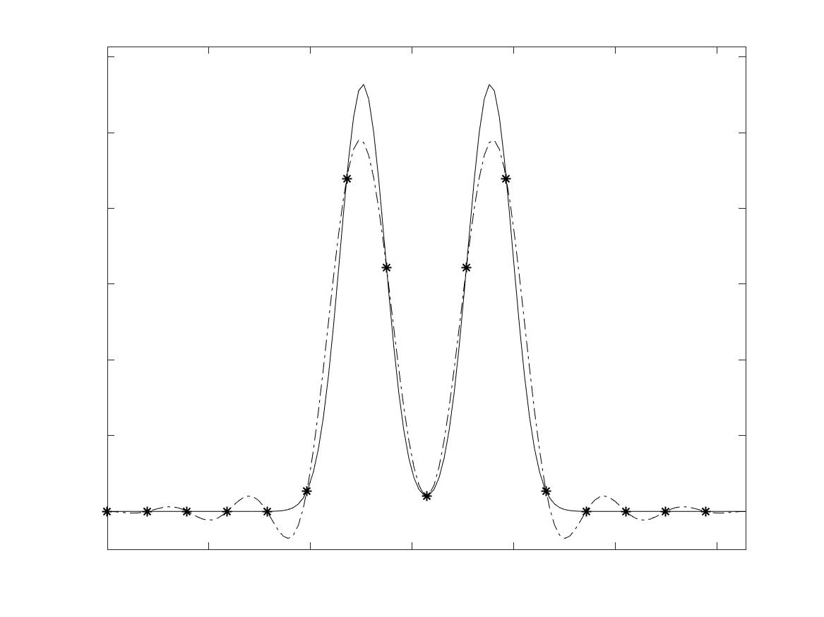
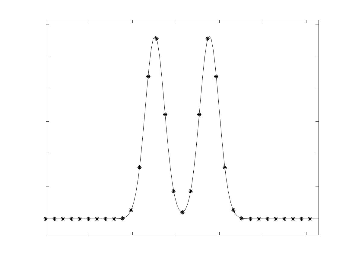
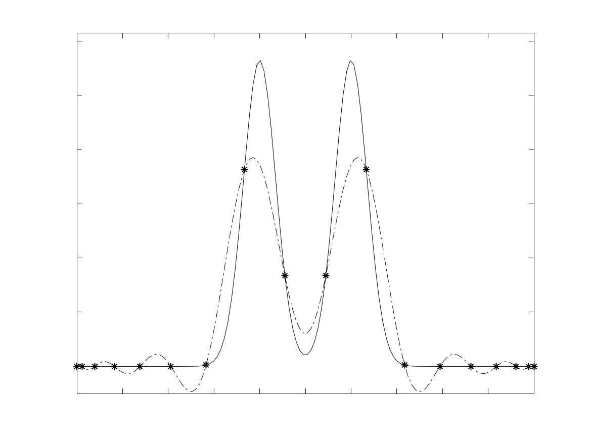
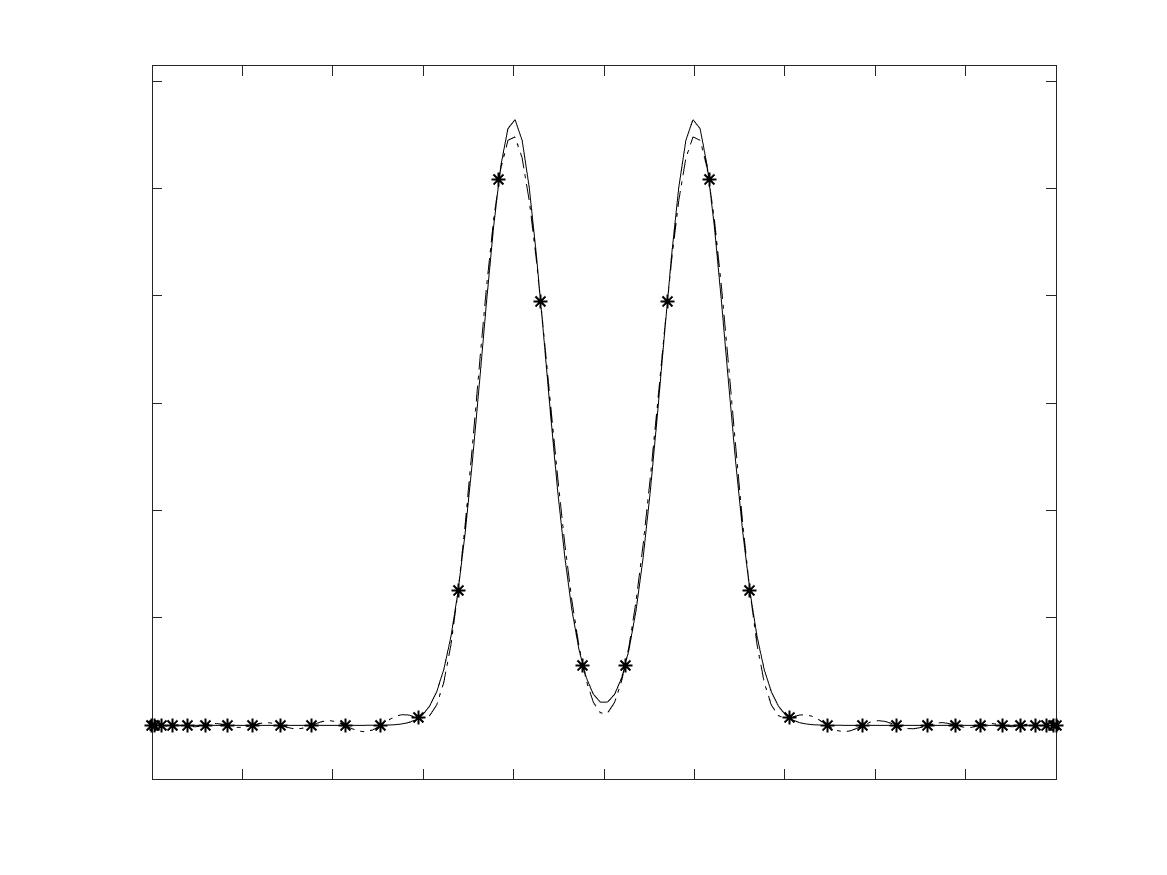
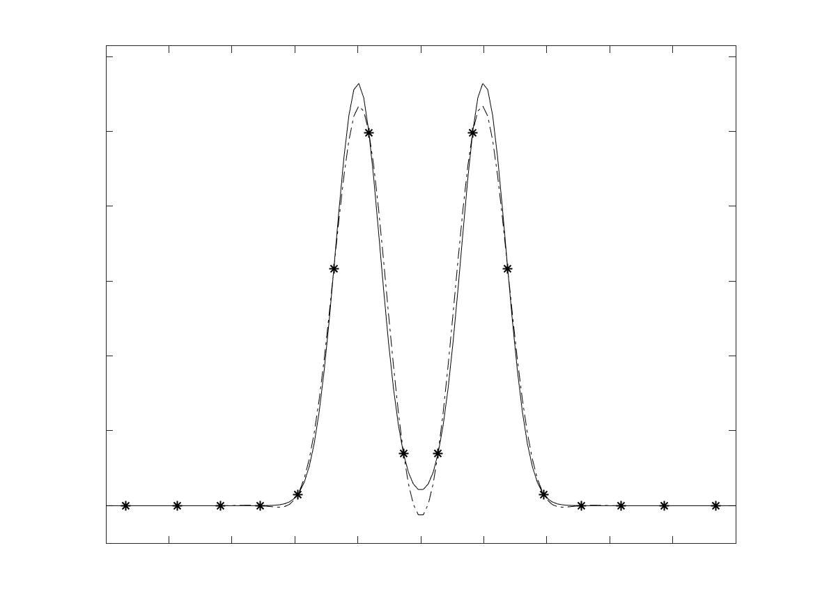
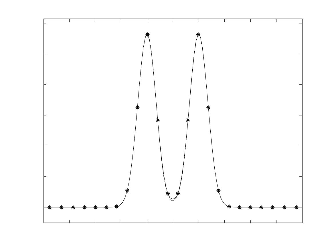
Figure 1: Interpolation with respect to $v\in[-5,5]$ of the function (52) with $M=2^{4}$ (left plots) or $M=2^{5}$ (right plots). After a suitable mapping of the nodes into the interval $[-5,5]$, the interpolations are relative to the Fourier case (top), the Legendre case (center) and the Hermite case (bottom).

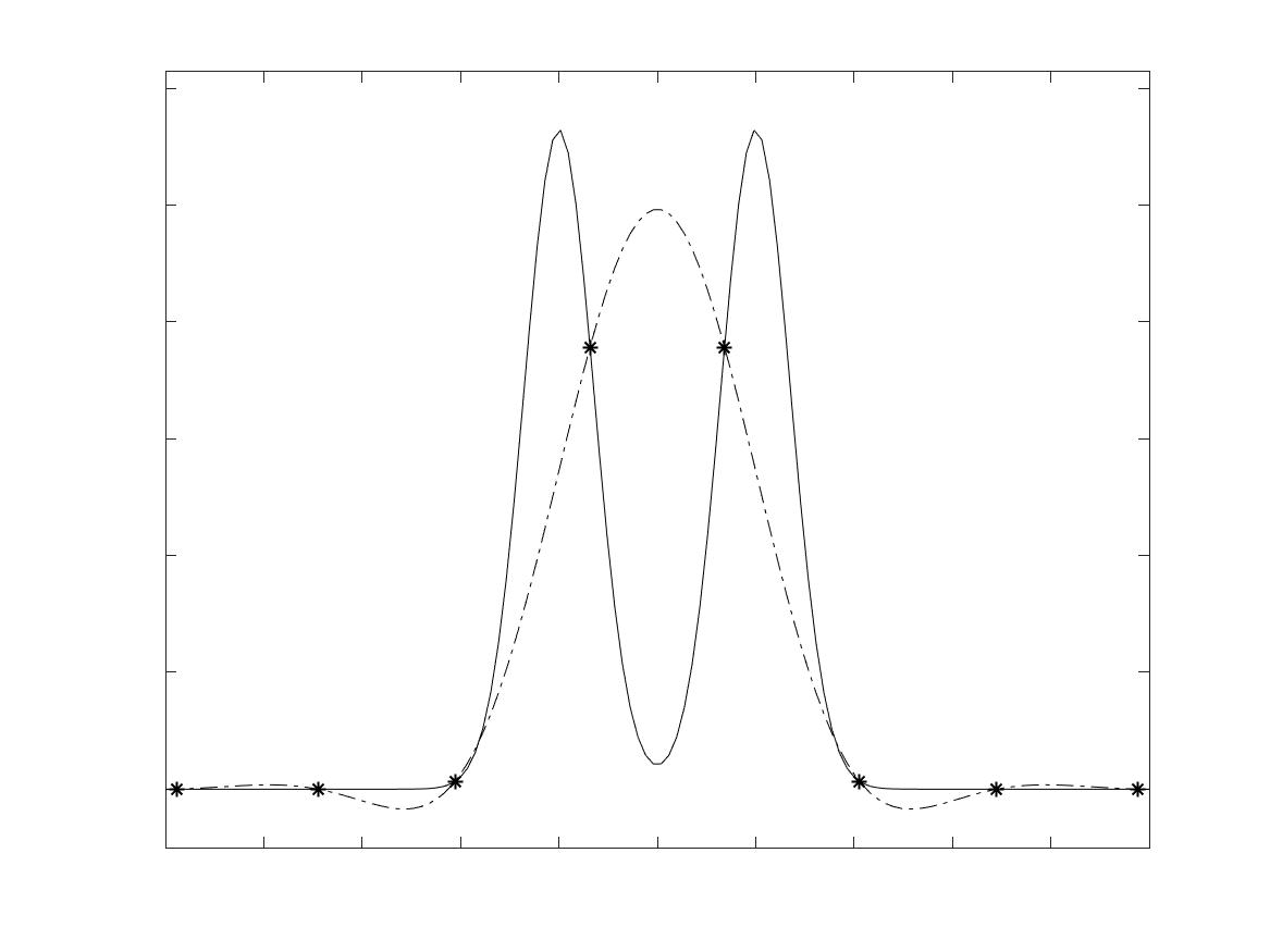
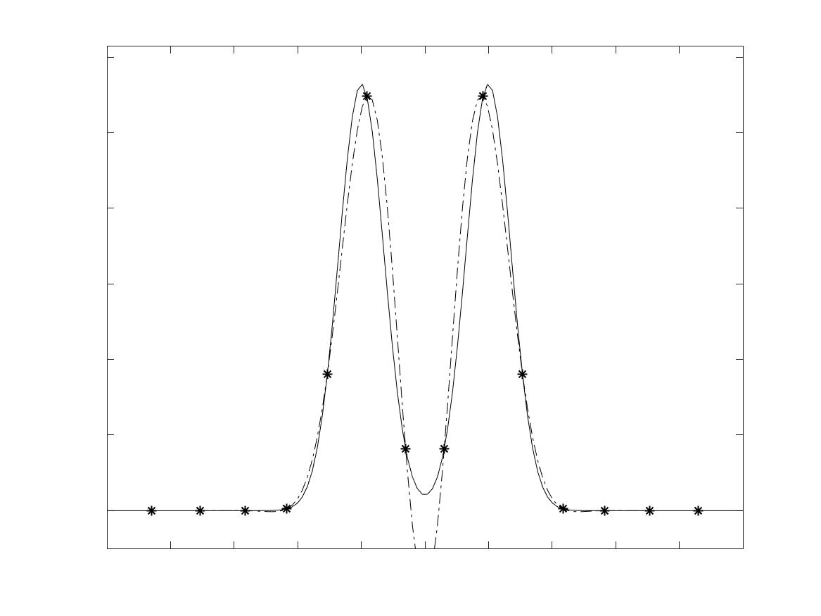
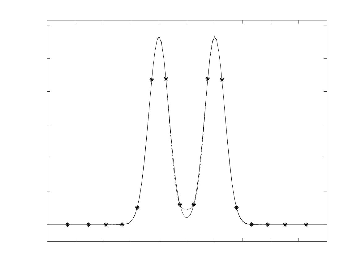
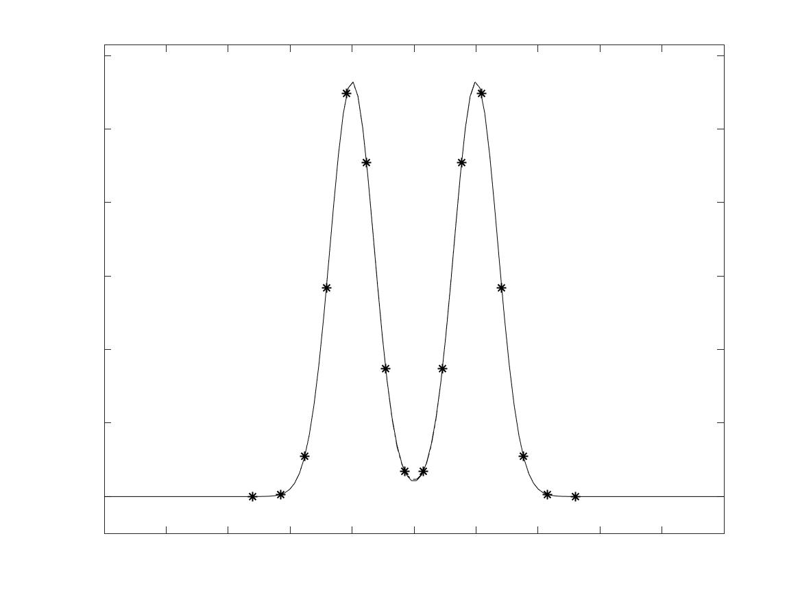
Figure 2: Interpolation with respect to $v\in[-5,5]$ of the function (52) with $M=2^{4}$. The interpolation is made using scaled Hermite nodes with $\alpha=0.4$ (top-left), $\alpha=0.9$ (top-right), $\alpha=1.1$ (bottom-left) and $\alpha=1.8$ (bottom-right).

6 Conservation Properties

The discrete counterpart of (6) (which is the law stating that the number of particles is preserved) holds for the scheme (35)-(36), when $g=0$. Of course, the conservation of this basic quantity is rather important from the physics viewpoint. At step $t^{k}=k\Delta t$, we define:

$$Q^{(k)}_{N,M}=\frac{2\pi}{N}\sum_{n=0}^{N-1}\sum_{m=0}^{M-1}c^{(k)}_{nm}w_{m}=\int_{\Omega}f^{(k)}_{N,M}(x,v)dxdv\approx\int_{\Omega}f(t^{k},x,v)dxdv,$$ (53)

where $w_{m}=2\pi/M$ in the periodic Fourier case (recall the quadrature formula (19)), while the weights are related to the quadrature formula (45), which are also valid for both Legendre and Hermite cases. From (35), at time step $t^{k+1}$ we find out that:

$$Q^{(k+1)}_{N,M}=\frac{2\pi}{N}\sum_{n=0}^{N-1}\sum_{m=0}^{M-1}\Big{(}c_{nm}^{(k)}+\Delta t\,\Phi_{nm}^{(k)}\Big{)}w_{m}=Q^{(k)}_{N,M}+\Delta Q^{(k)}_{N,M}=Q^{(k)}_{N,M}.$$ (54)

In fact, one has:

$$\Delta Q^{(k)}_{N,M}=-\Delta t\sum_{m=0}^{M-1}v_{m}\left[\int_{\Omega_{x}}\frac{\partial f^{(k)}_{N,M}}{\partial x}(x,v_{m})dx\right]\frac{w_{m}}{\omega(v_{m})}$$

$$+\ \Delta t\frac{2\pi}{N}\sum_{n=0}^{N-1}E^{(k)}_{N}(x_{n})\left[\int_{\Omega_{v}}\frac{\partial f^{(k)}_{N,M}}{\partial v}(x_{n},v)dv\right]=0,$$ (55)

where $\omega(v)=1$ in the trigonometric and in the Legendre case, while $\omega(v)=\exp(-v^{2})$ in the Hermite case. The integrals above are zero as a consequence of the boundary conditions. This is true for all the cases we are considering in this paper, i.e., periodic boundary conditions or homogeneous Dirichlet conditions (imposed at the points $\pm 1$ when $\Omega_{v}=]-1,1[$ or through a suitable exponential decay when $\Omega_{v}=\mathbb{R}$). In the end, we proved that the quantity in (53) does not change passing from $k$ to $k+1$. The same property holds for the scheme (4). The proof follows after recognizing that, for $g=0$, one has:

$$Q^{(k+1)}_{N,M}=\frac{4}{3}Q^{(k)}_{N,M}-\frac{1}{3}Q^{(k-1)}_{N,M}.$$ (56)

The above recurrence relation provides constant values when the initial coefficients are such that $c^{(1)}_{ij}=c^{(0)}_{ij}$.

Analogous considerations are made regarding the conservation in time of the momenta $\int_{\Omega}v^{r}f(t,x,v)dxdv$, where $r\geq 0$ is an integer. In the discrete case we define at time $t^{k}$, $k=0,1,\ldots,K$:

$$Q^{(k)}_{N,M,r}=\frac{2\pi}{N}\sum_{n=0}^{N-1}\sum_{m=0}^{M-1}v_{m}^{r}c^{(k)}_{nm}w_{m}\approx\int_{\Omega}v^{r}f^{(k)}_{N,M}(x,v)dxdv.$$ (57)

Of course $Q^{(k)}_{N,M,0}=Q^{(k)}_{N,M}$. We expect conservation of the discrete momenta in the Legendre or Hermite case, for values of $r$ up to the integration capabilities of Gaussian formulas. This means $r\leq M$ for the Legendre case and $r\leq M+2$ for the Hermite case. We note instead that, being $v$ not a trigonometric function, the integration formula does not hold in the periodic case. In this situation, $v$ can be substituted by its projection in the $L^{2}(\Omega)$ norm on the finite dimensional space ${\bf Y}_{N,M}$, up to an error that decays spectrally. This procedure may however generate a Gibb’s phenomenon across the points of $\Omega$ with $v=2\pi$, where $v^{r}f$ is discontinuous. Nevertheless, if the function $f$ shows a fast decay near the boundary with respect to the variable $v$, the conservation of momenta can be achieved up to negligible errors.

At time $t^{k}$, $k=0,1,\ldots,K$, we can also consider the discrete version of (7) i.e.:

$${\cal E}(t^{k})\approx{\cal E}^{(k)}_{N,M}=\frac{1}{2}\left(\frac{2\pi}{N}\sum_{n=0}^{N-1}\sum_{m=0}^{M-1}v^{2}_{m}c^{(k)}_{nm}w_{m}+\frac{2\pi}{N}\sum_{n=0}^{N-1}\Big{[}E^{(k)}_{N}(x_{n})\Big{]}^{2}\right).$$ (58)

that includes the term $Q^{(k)}_{N,M,2}$. Conservation properties of this quantity will be tested later in the numerical section.

7 Numerical experiments

Together with other notable examples, the numerical scheme here proposed has been already validated in  [25] in the case of the two-stream instability example, which is a standard benchmark for plasma physics codes. This corresponds to the setting $\Omega_{x}=[0,4\pi[$, $\Omega_{v}=[-5,5]$ in (1), (2), (3), (4), with the initial guess given by:

$$\bar{f}(x,v)=\frac{1}{2a\sqrt{2\pi}}\left[\exp{\left(-\frac{v-\beta}{a\sqrt{2}}\right)^{2}}+\exp{\left(-\frac{v+\beta}{a\sqrt{2}}\right)^{2}}\right]\left[1+\epsilon\cos\left(\kappa x\right)\right],$$ (59)

with $a=1/{\sqrt{8}}$, $\beta=1$, $\epsilon=10^{-3}$, $\kappa=0.5$. The exact solution is approximated by periodic basis functions in the variable $x$ and Fourier, Legendre and Hermite basis functions in the variable $v$. For practical purposes, depending the basis examined, we rewrite the differential equation on the domain $\Omega=[0,2\pi[\times\Omega_{v}$, with $\Omega_{v}=[0,2\pi[$ (Fourier) or $\Omega_{v}=]-1,1[$ (Legendre), while $\Omega_{v}=\mathbb{R}$ is not modified in the Hermite case. The purpose of the paper is to discuss the different performances in dependence of the basis used for the variable $v$. Comparisons between the various approaches are made by taking less degrees of freedom than those actually necessary to resolve accurately the equation. In particular, we will perform experiments by setting $N=M=2^{4}$.

In all the experiments to follow, we integrate up to time $T=30$ using the second-order BDF scheme with an appropriate time step, in order to guarantee stability. The choice of an accurate time discretization procedure will allow us to concentrate our attention to the spectral approximation in the variable $x$ and $v$. First of all, in Figure 4 we show the results at time $T=25$ and time $T=30$ of the solution recovered by the Fourier-Fourier method, by choosing $N=2^{5}$, $M=2^{6}$ and a rather small time step ($\Delta t=0.25\cdot 10^{-2}$). This will be the referring figure for the successive comparisons.

Figure 4 shows the time evolution of $|\hat{a}_{1}^{(k)}|$, which is the first Fourier mode of the electric field $E^{(k)}_{N}$ in (31), when the Fourier-Fourier method with $N=2^{5}$, $M=2^{6}$ and $\Delta t=1/800$ is used. This crucial quantity is often displayed in order to make comparisons between computational codes, also because its behavior is predicted by theoretical consideration. Indeed, the slope of the segment starting from $T=15$ in the plot of Figure 4 agrees with the expectancy [7, Chapter 5].

The plots of Figure 5 show the numerical distribution at time $T=25$ and time $T=30$ obtained by using the Fourier-Fourier method with $N=M=2^{4}$ and $\Delta t=0.01$. Such an approximation is rough, but the computation is stable and provides an idea of the real behavior. Unfortunately, as we predicted in Section 5, results of this kind are not available for the Fourier-Legendre case. The algorithm is stable up to $T=25$ (see Figure 6), but then it explodes. As we already mentioned, the explanation of this fact may rely on the poor approximation of the Legendre interpolants at the interior of the interval. The performances improve relevantly by increasing the value of $M$. The Fourier-Fourier method looks however a better choice, by virtue also of the fact that it allows for the use of the DFT.

The results concerning the use of Hermite function deserve a deeper discussion. Figure 7 shows the numerical distribution at time $T=25$ and time $T=30$ obtained by using the Fourier-Hermite method with $N=M=2^{4}$, $\Delta t=0.01$ and $\alpha=1$. Besides, in Figure 8 we display the approximated solution at time $T=25$ and time $T=30$ obtained with the same parameters (i.e. $N=M=2^{4}$, $\Delta t=0.01$) and different values of the parameter $\alpha$. Figure 9 shows the approximated distribution function at time $T=30$ when $x=0$, obtained by using Fourier-Hermite method with $N=M=2^{4}$, $\Delta t=0.01$ for various $\alpha$. These figures point out that the approximated solution is very sensitive to the choice of $\alpha$. It has to be noted, however, that the parameter $\alpha$ that well performs for the initial datum (59) does not necessarily behave optimally as time increases. For example, the value $\alpha=1.8$ looks the best choice for the approximation of the initial distribution (see Figure 2 on bottom), nevertheless, keeping $\alpha$ constantly equal to such a value brings to instability before arriving at time $T=30$. This behavior clearly suggests that a dynamical way to vary $\alpha$ during the computations should be recommended, though there are at the moment no reasonable ideas on how to realize it in practice.

In Figure 10 we plot the time evolution of the (log of the) first Fourier mode of the electric field $E^{(k)}_{N}$, i.e. $|\hat{a}_{1}^{(k)}|$ in  (31), when the Fourier-Fourier method (top) and the Fourier-Hermite method (bottom) with $N=M=2^{4}$, $\Delta t=0.01$ and $\alpha=1$ are used. If we compare with Figure 4, the two plots behave rather differently, being the second much better that the first one.

In all the numerical experiments the number of particles $Q^{(k)}_{N,M}$ and the momentum $P^{(k)}_{N,M}$ defined in  (53) and  (57) are preserved. The situation is slightly different concerning the energy, where a slight growth is observed, with a rate depending on the size of the time step. Therefore, we conclude our series of tests by showing in Figures 12 and 12 the variation versus time (in a semi-$\log$ diagram) of the following quantity:

$$\frac{\left|\mathcal{E}_{N,M}^{(k)}-\mathcal{E}_{N,M}^{(0)}\right|}{\left|\mathcal{E}_{N,M}^{(0)}\right|},$$ (60)

where the discrete energy $\mathcal{E}_{N,M}^{(k)}$, is defined in (58). Regarding energy conservation, for the same resolution in the phase space ($N=M=2^{4}$) and time ($\Delta t=0.001$), the performance of the Fourier-Hermite method examined in this work is superior to that of the Fourier-Fourier method studied in [25].

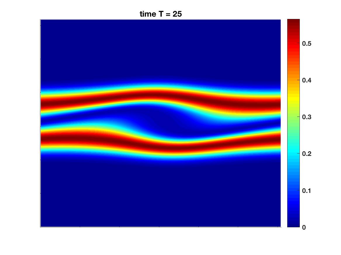
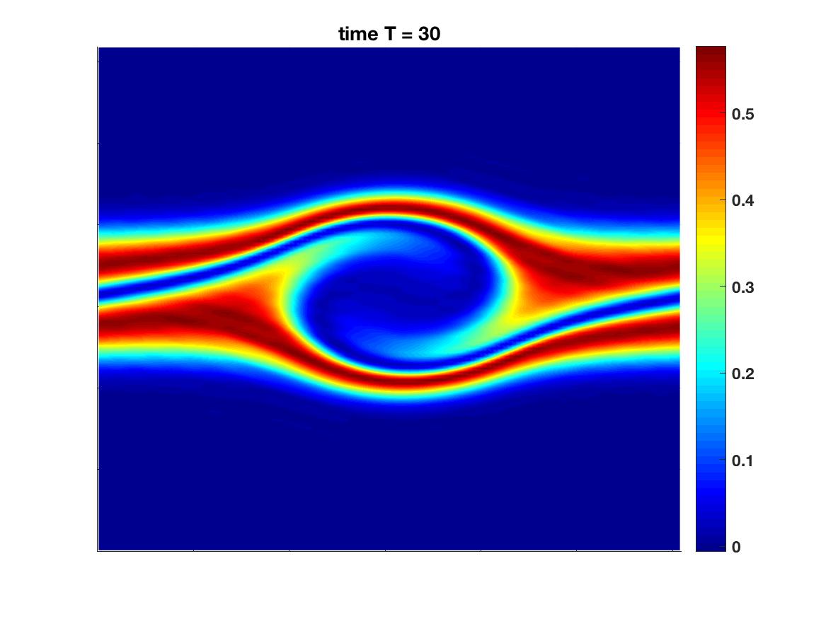
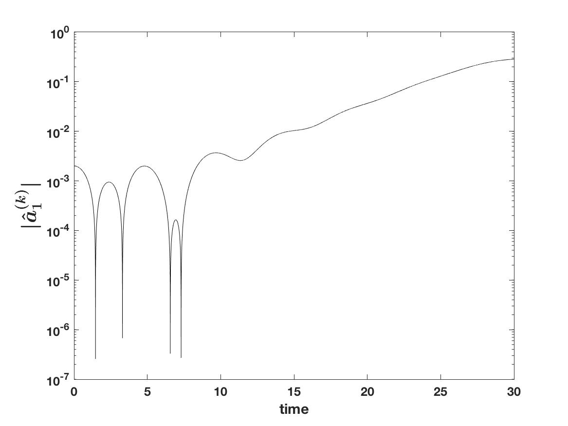
Figure 3: Approximated distribution function obtained by using the Fourier-Fourier method with $N=2^{5}$, $M=2^{6}$ and $\Delta t=1/800$.

Figure 4: Time evolution of the first Fourier mode of the electric field $E^{(k)}_{N}$, i.e. $|\hat{a}_{1}^{(k)}|$ in (31) when using the Fourier-Fourier method for $N=2^{5}$, $M=2^{6}$ and $\Delta t=1/800$.

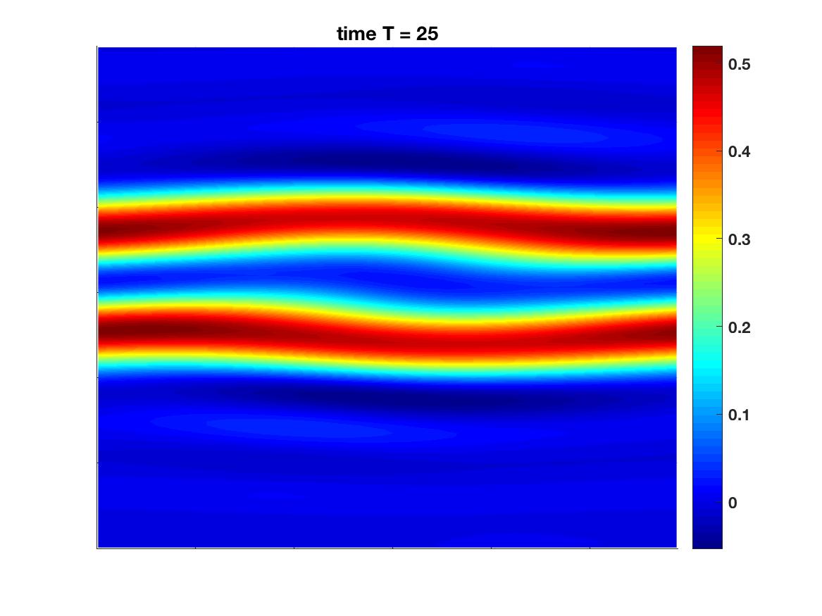
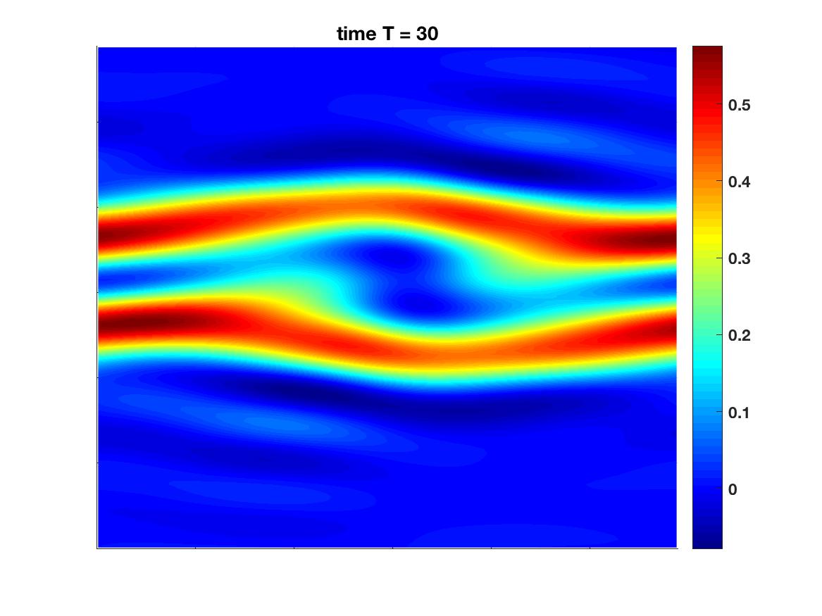
Figure 5: Approximated distribution function obtained by using the Fourier-Fourier method with $N=M=2^{4}$ and $\Delta t=0.01$.

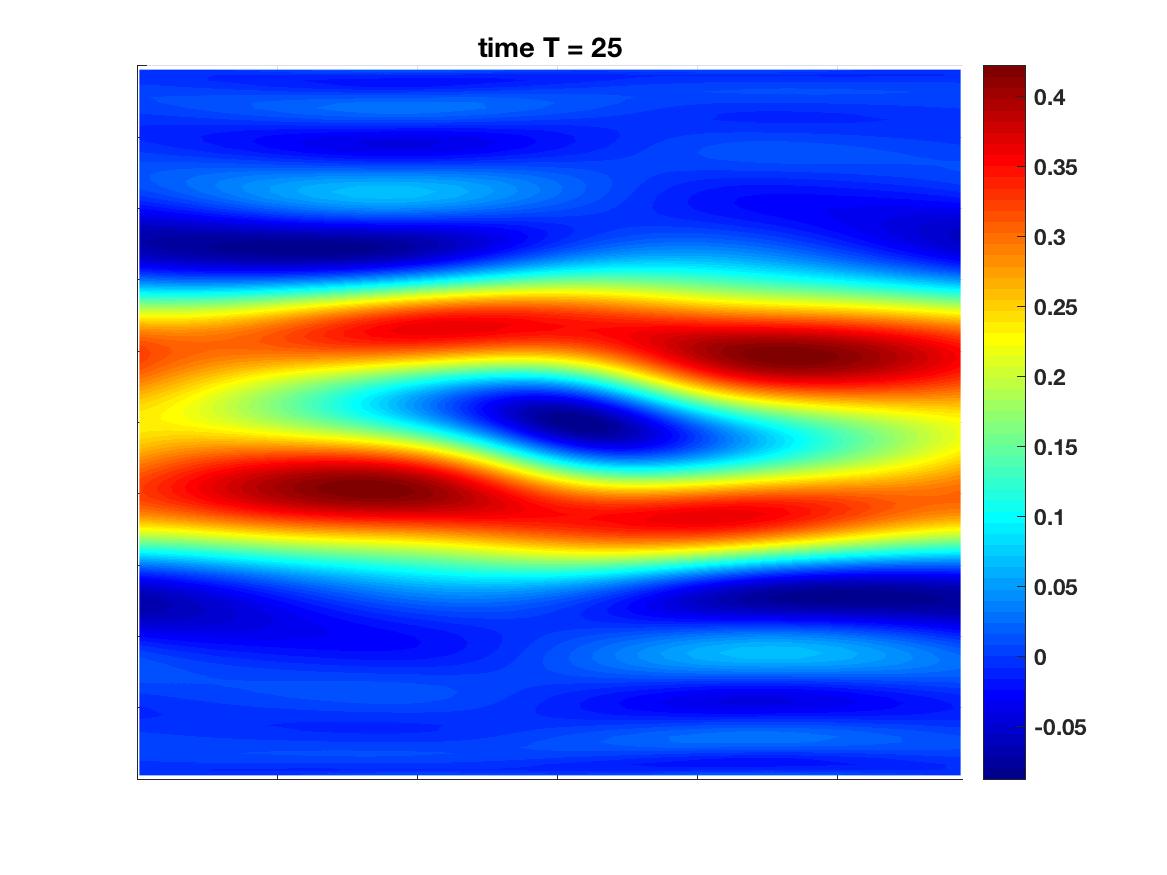
Figure 6: Approximated distribution function obtained by using the Fourier-Legendre method with $N=M=2^{4}$ and $\Delta t=0.01$.

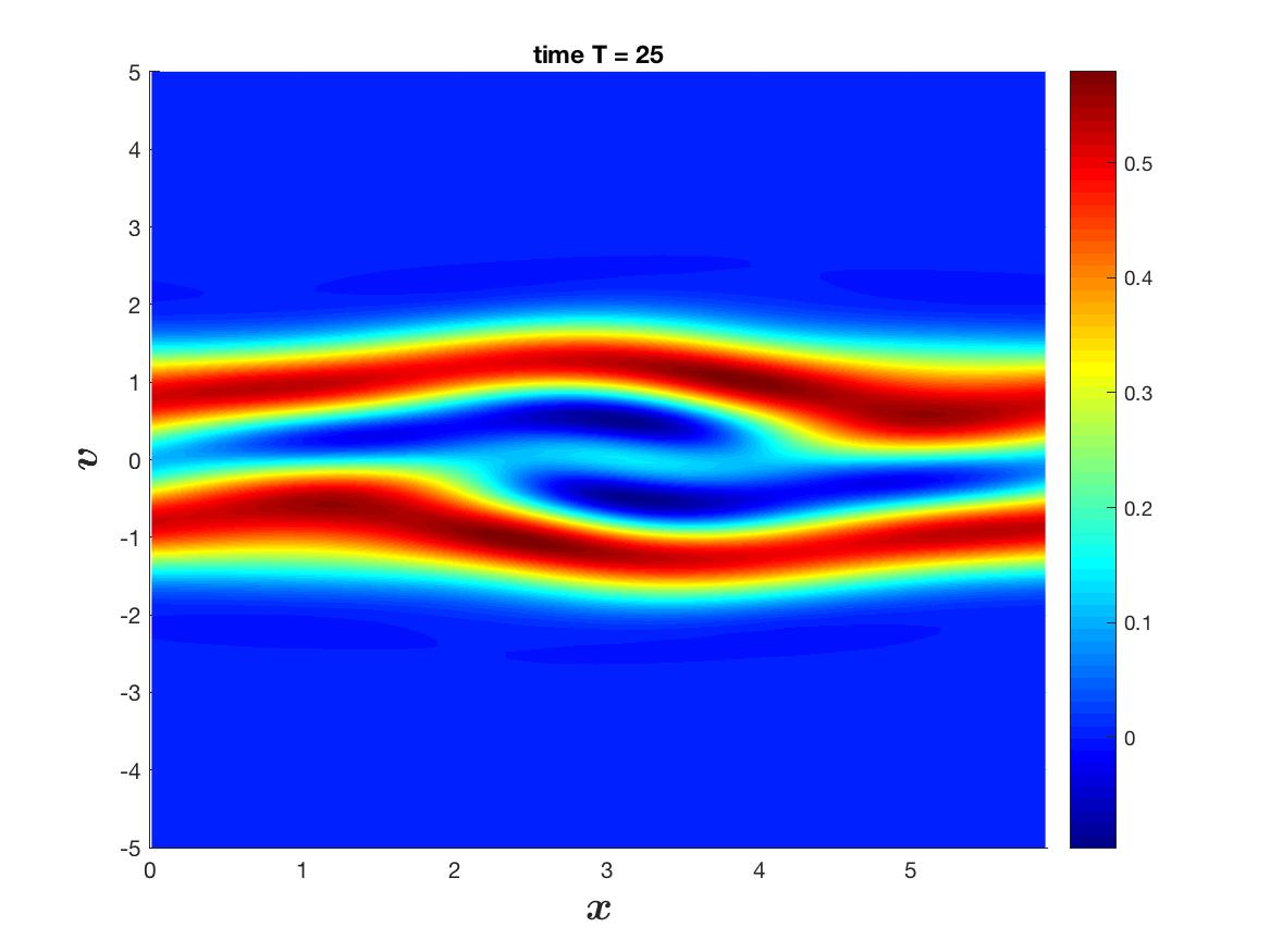
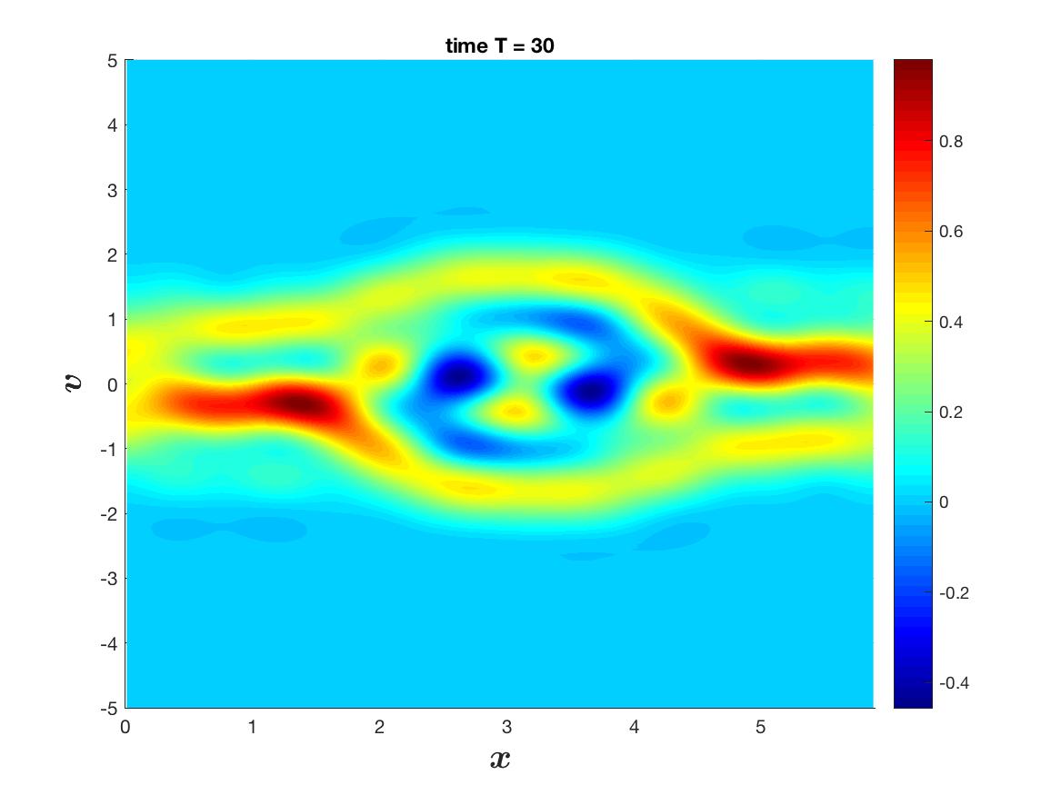
Figure 7: Approximated distribution function obtained by using the Fourier-Hermite method with $N=M=2^{4}$, $\Delta t=0.01$ and $\alpha=1$ .

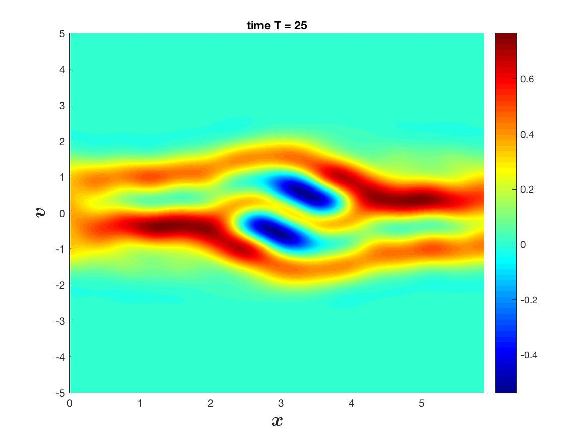
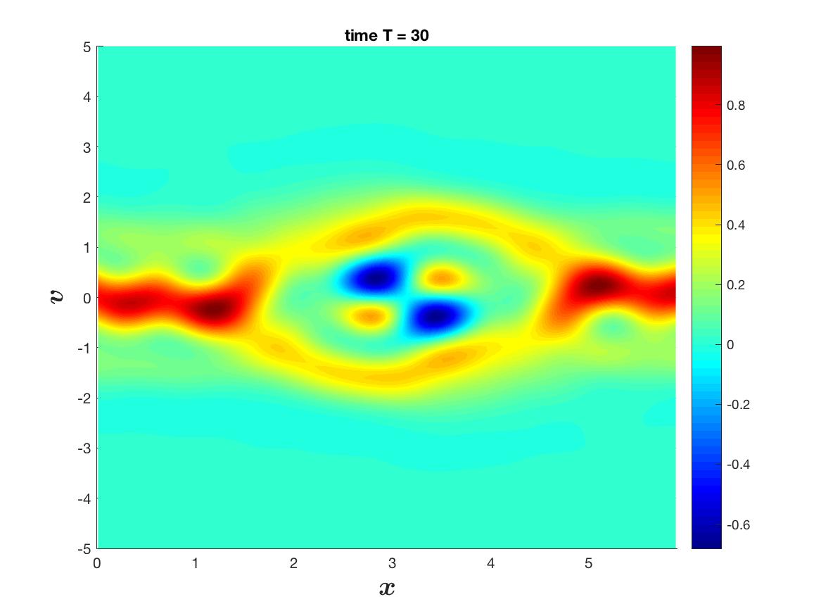
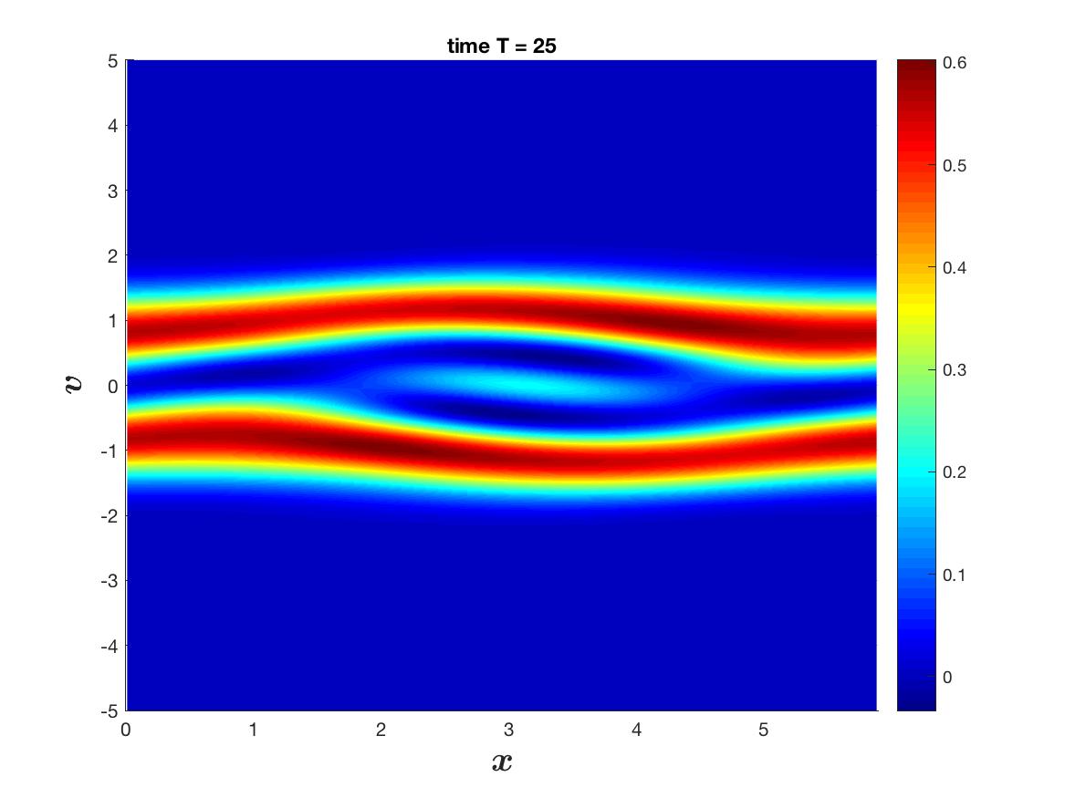
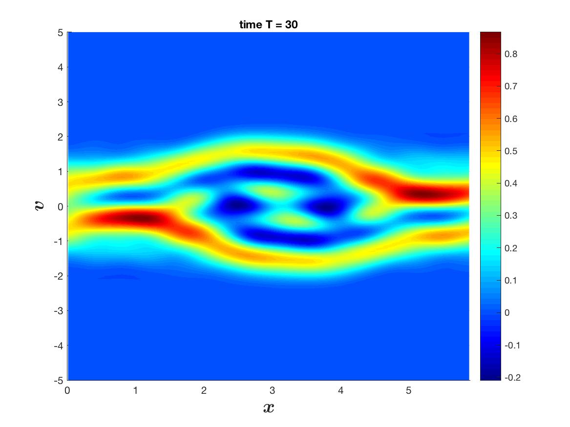
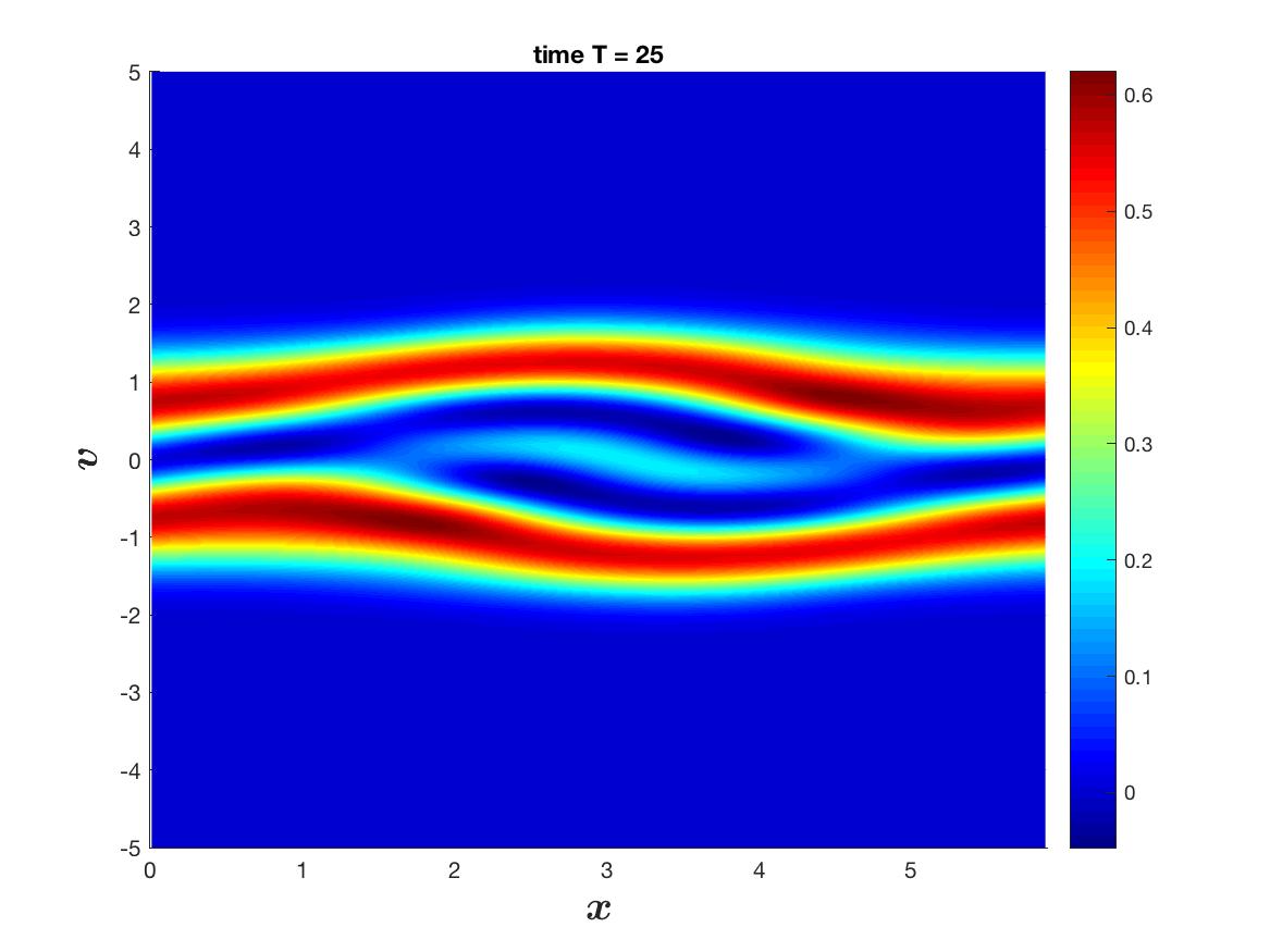
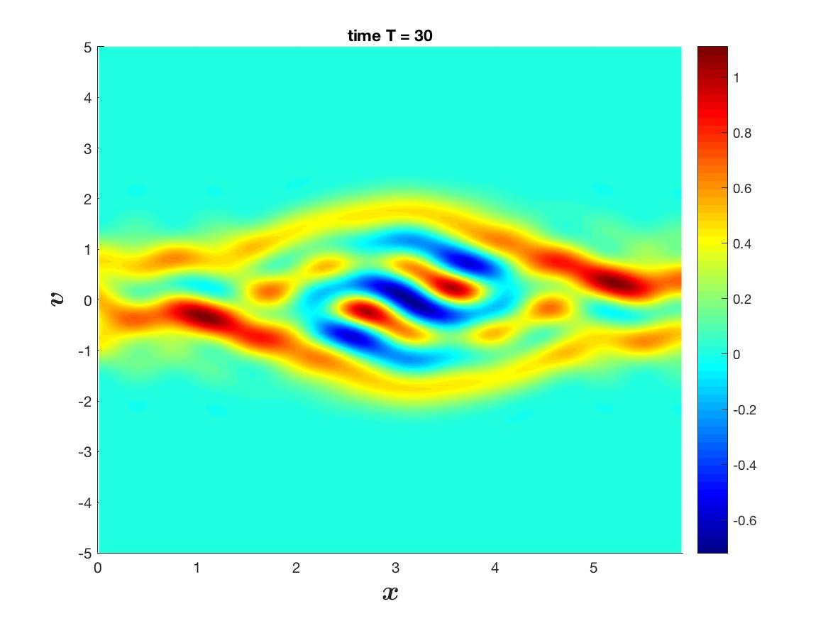
Figure 8: Approximated distribution function obtained by using the Fourier-Hermite method with $N=M=2^{4}$, $\Delta t=0.01$ and $\alpha=0.9$ (top), $\alpha=1.1$ (center), $\alpha=1.2$ (bottom).

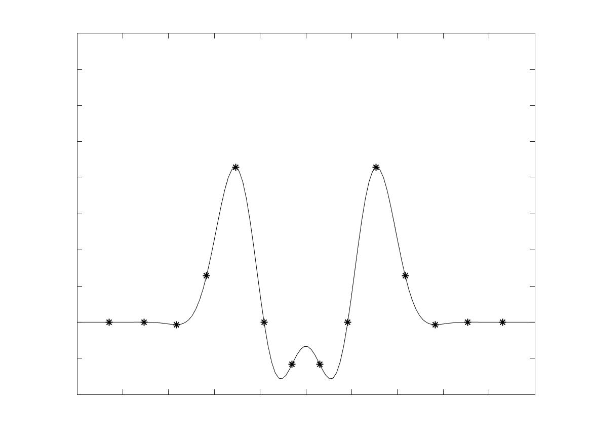
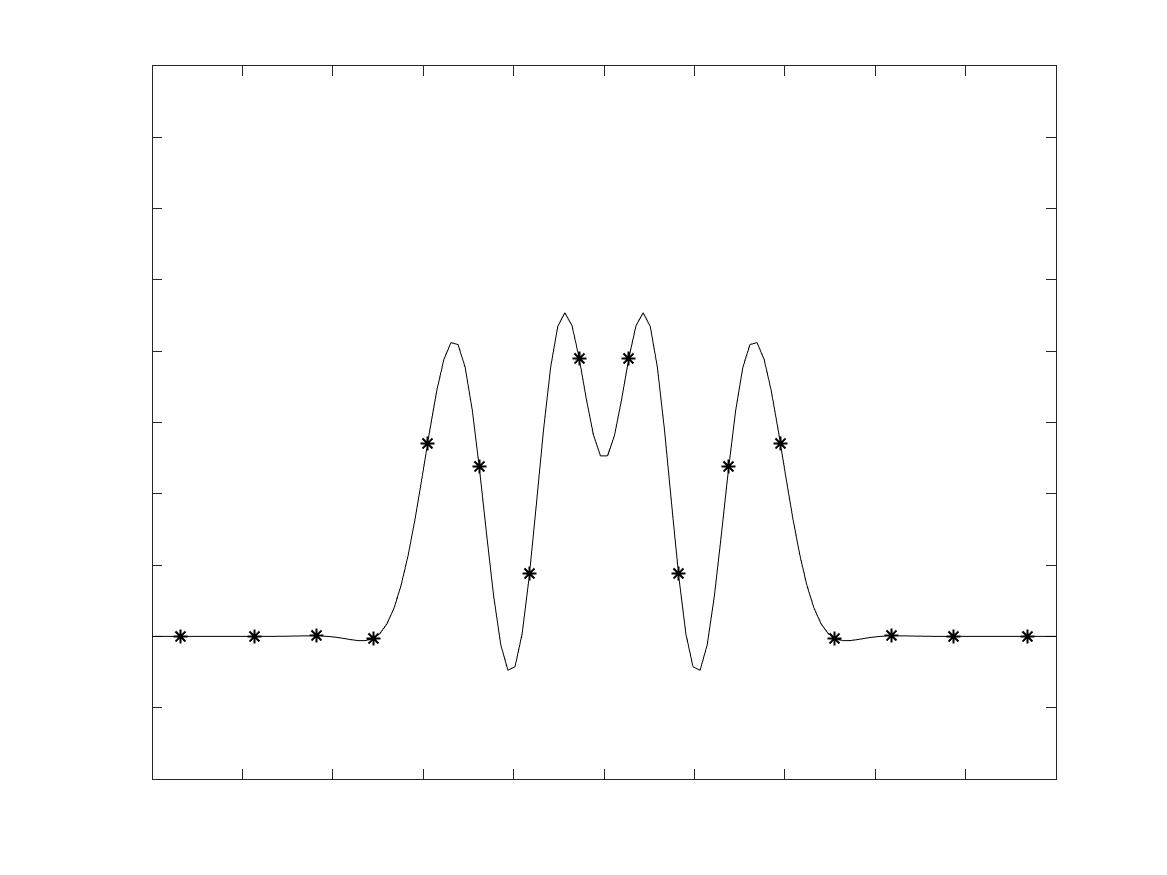
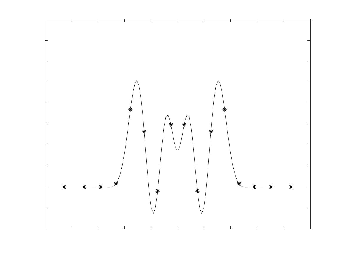
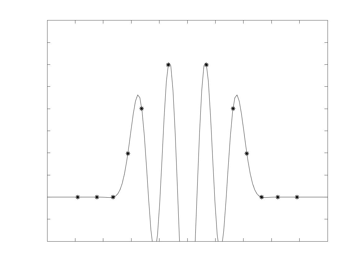
Figure 9: Approximated distribution function in the variable $v$ at time $T=30$ when $x=0$, obtained by using the Fourier-Hermite method with $N=M=2^{4}$, $\Delta t=0.01$ and $\alpha=0.9$ (top-left), $\alpha=1$ (top-right), $\alpha=1.1$ (bottom-left) and $\alpha=1.2$ (bottom-right).

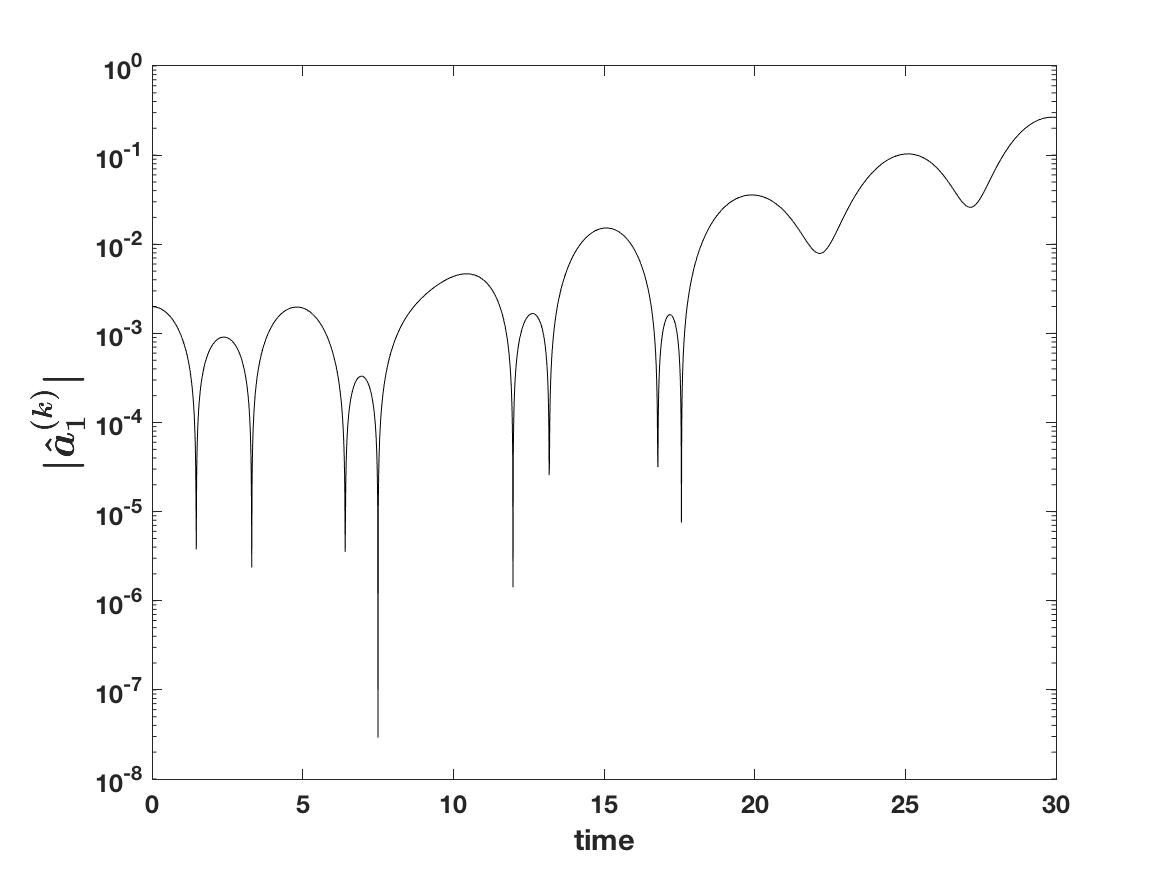
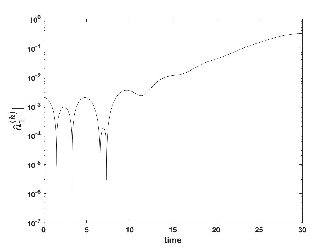
Figure 10: Time evolution of the first Fourier mode of the electric field $E^{(k)}_{N}$, i.e. $|\hat{a}_{1}^{(k)}|$ in (31), when using the Fourier-Fourier method (left) and the Fourier-Hermite method (right) with $N=M=2^{4}$, $\Delta t=0.01$ and $\alpha=1$.

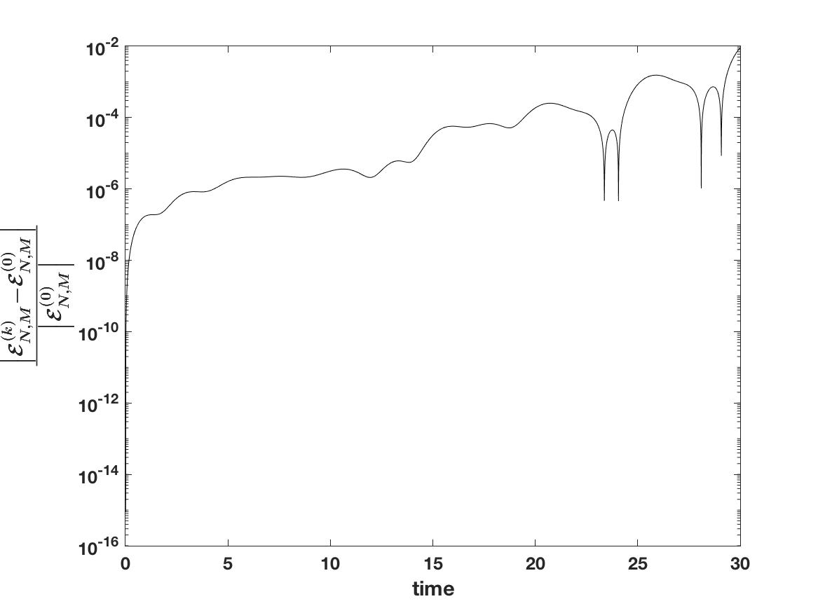
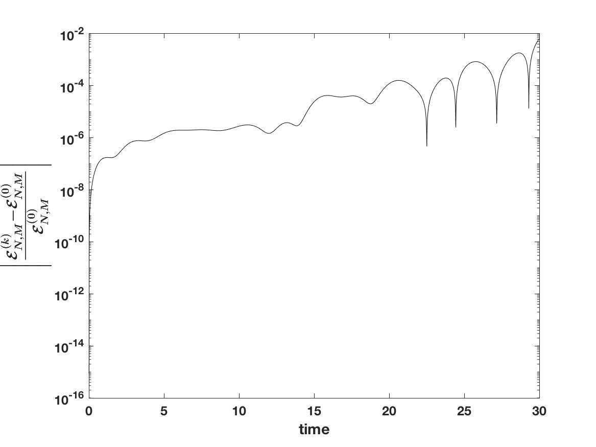
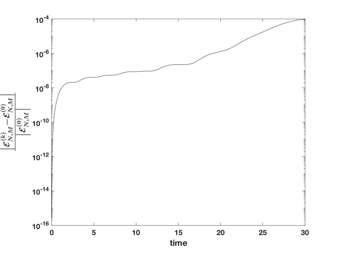
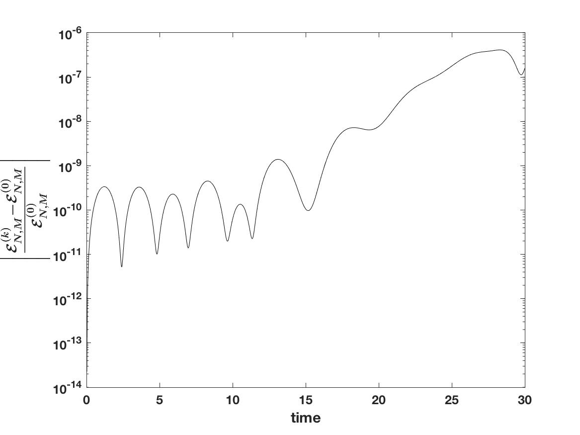
Figure 11: Growth of the total energy using the first-order one-step Fourier-Fourier scheme (left) and the second-order BDF Fourier-Fourier scheme (right) with $N=M=2^{4}$, and $\Delta t=0.01$.

Figure 12: Growth of the total energy using the first-order one-step Fourier-Hermite scheme (left) and the second-order BDF Fourier-Hermite scheme (right) with $N=M=2^{4}$, $\Delta t=0.01$ and $\alpha=1$.

8 Conclusions

In this work, we extended the semi-Lagrangian spectral method developed in [25], by implementing Legendre polynomials and Hermite functions to approximate the distribution function with respect to the velocity variable. In particular, we discussed second-order accurate-in-time semi-Lagrangian methods, obtained by coupling spectral techniques in the space-velocity domain with a BDF time-stepping scheme. The resulting numerical code possesses good conservation properties, which have been assessed by a series of numerical tests conducted on the standard two-stream instability benchmark problem. We also investigated numerically the dependence of the Fourier-Hermite approximations on the scaling parameter in the Gaussian weight. Our experiments for different representative values of this parameter confirm that a proper choice may significantly impact on accuracy, thus confirming previous results from the literature. The next step would be the development of a strategy for the automatic set up of the parameter during the time-advancing procedure.

References

- [1] T. D. Arber and R. G. L. Vann. A critical comparison of Eulerian-grid-based Vlasov solvers. Journal of Computational Physics, 180:339–357, 2002.
- [2] B. Ayuso, J. A. Carrillo, and C.-W. Shu. Discontinuous Galerkin methods for the one-dimensional Vlasov-Poisson system. Kinetic & Related Models, 4(4):955–989, 2011.
- [3] B. Ayuso, J. A. Carrillo, and C.-W. Shu. Discontinuous Galerkin methods for the multi-dimensional Vlasov-Poisson problem. Mathematical Models and Methods in Applied Sciences, 22(12):1250042, 2012.
- [4] J. W. Banks and J. A. F. Hittinger. A new class of nonlinear finite-volume methods for Vlasov simulation. IEEE Transactions on Plasma Science, 38(9):2198–2207, Sept 2010.
- [5] C. Bernardi and Y. Maday. Spectral methods. In P. Ciarlet and J. Lions, editors, Handbook of Numerical Analysis, pages 209–486. Elsevier, Amsterdam, 1997.
- [6] C. K. Birdsall and A. B. Langdon. Plasma physics via computer simulation. Taylor & Francis, New York, 1st edition, 2005.
- [7] J. A. Bittencourt. Fundamentals of Plasma Physics. Springer-Verlag New York, 3 edition, 2004.
- [8] J. P. Boyd. The rate of convergence of Hermite function series. Mathematics of Computation, 35:1309–1316, 1980.
- [9] J. P. Boyd. Asymptotic coefficients of Hermite function series. Journal of Computational Physics, 54:382–410, 1984.
- [10] J. P. Boyd. Chebyshev and Fourier Spectral Methods. Springer, Berlin, 1989.
- [11] T. J. M. Boyd and J. J. Sanderson. The Physics of Plasmas. Cambridge University Press, 2003.
- [12] J. U. Brackbill. On energy and momentum conservation in particle-in-cell plasma simulation. Journal of Computational Physics, 317:405–427, 2016.
- [13] E. Brigham. The fast Fourier transform and its applications. Prentice Hall, 1st edition, 1988.
- [14] E. Camporeale, G. L. Delzanno, B. K. Bergen, and J. D. Moulton. On the velocity space discretization for the Vlasov-Poisson system: comparison between Hermite spectral and Particle-in-Cell methods. Part 2: fully-implicit scheme. Computer Physics Communications, 198:47–58, 2016.
- [15] E. Camporeale, G. L. Delzanno, G. Lapenta, and W. Daughton. New approach for the study of linear Vlasov stability of inhomogeneous systems. Physics of Plasmas, 13(9):092110, 2006.
- [16] C. Canuto, M. Y. Hussaini, A. M. Quarteroni, and T. A. J. Zang. Spectral Methods in Fluid Dynamics. Scientific Computation. Springer-Verlag, Berlin Heidelberg, first edition, 1988.
- [17] J. A. Carrillo and F. Vecil. Nonoscillatory interpolation methods applied to Vlasov-based models. SIAM Journal on Scientific Computing, 29(3):1179–1206, 2007.
- [18] G. Chen and L. Chacon. A multi-dimensional, energy- and charge-conserving, nonlinearly implicit, electromagnetic Vlasov-Darwin particle-in-cell algorithm. Computer Physics Communications, 197:73–87, 2015.
- [19] G. Chen, L. Chacon, and D. Barnes. An energy- and charge-conserving, implicit, electrostatic particle-in-cell algorithm. Journal of Computational Physics, 230(18):7018–7036, 2011.
- [20] C. Z. Cheng and G. Knorr. The integration of the Vlasov equation in configuration space. Journal of Computational Physics, 22(3):330–351, 1976.
- [21] A. Christlieb, W. Guo, M. Morton, and J.-M. Qiu. A high order time splitting method based on integral deferred correction for semi-Lagrangian Vlasov simulations. Journal of Computational Physics, 267:7–27, 2014.
- [22] G. H. Cottet and P.-A. Raviart. Particle methods for the one-dimensional Vlasov-Poisson equations. SIAM Journal on Numerical Analysis, 21(1):52–76, 1984.
- [23] N. Crouseilles, T. Respaud, and E. Sonnendrücker. A forward semi-Lagrangian method for the numerical solution of the Vlasov equation. Computer Physics Communications, 180(10):1730–1745, 2009.
- [24] G. L. Delzanno. Multi-dimensional, fully-implicit, spectral method for the Vlasov-Maxwell equations with exact conservation laws in discrete form. Journal of Computational Physics, 301:338–356, 2015.
- [25] D. Fatone, L. Funaro and G. Manzini. Arbitrary-order time-accurate semi-Lagrangian spectral approximations of the Vlasov-Poisson system. arXiv:1803.09305 [math.NA], 2018.
- [26] F. Filbet. Convergence of a finite volume scheme for the Vlasov-Poisson system. SIAM Journal on Numerical Analysis, 39(4):1146–1169, 2001.
- [27] F. Filbet and E. Sonnendrücker. Comparison of Eulerian Vlasov solvers. Computer Physics Communications, 150(3):247–266, 2003.
- [28] F. Filbet, E. Sonnendrücker, and P. Bertrand. Conservative numerical schemes for the Vlasov equation. Journal of Computational Physics, 172(1):166–187, 2001.
- [29] Funaro. Polynomial Approximation of Differential Equations. Springer, 1992.
- [30] D. Funaro and O. Kavian. Approximation of some diffusion evolution equations in unbounded domains by Hermite functions. Mathematics of Computation, 57:597–619, 1990.
- [31] H. Gajewski and K. Zacharias. On the convergence of the Fourier-Hermite transformation method for the Vlasov equation with an artificial collision term. Journal of Mathematical Analysis and Applications, 61(3):752–773, 1977.
- [32] R. Glassey. The Cauchy Problem in Kinetic Theory. Society for Industrial and Applied Mathematics, 1996.
- [33] D. Gottlieb and S. A. Orszag. Numerical Analysis of Spectral Methods: Theory and Applications. Society for Industrial and Applied Mathematics, 1977.
- [34] H. Grad. On the kinetic theory of rarefied gases. Communications on Pure and Applied Mathematics, 2(4):331–407, 1949.
- [35] B.-y. Guo. Spectral Methods and Their Applications. World Scientific, Singapore, 1998.
- [36] B.-y. Guo. Error estimation of Hermite spectral method for nonlinear partial differential qquations. Mathematics of Computation, 68(227):1067–1078, 1999.
- [37] B.-y. Guo, J. Shen, and C.-l. Xu. Spectral and pseudospectral approximations using Hermite functions: Application to the Dirac equation. Advances in Computational Mathematics, 19(1):35–55, 2003.
- [38] B.-y. Guo and C.-l. Xu. Hermite pseudospectral method for nonlinear partial differential equations. ESAIM: Mathematical Modelling and Numerical Analysis, 34(4):859–872, 2000.
- [39] R. E. Heath, I. M. Gamba, P. J. Morrison, and C. Michler. A discontinuous Galerkin method for the Vlasov-Poisson system. Journal of Computational Physics, 231(4):1140–1174, 2012.
- [40] J. P. Holloway. Spectral velocity discretizations for the Vlasov-Maxwell equations. Transport Theory and Statistical Physics, 25(1):1–32, 1996.
- [41] A. J. Klimas. A numerical method based on the Fourier-Fourier transform approach for modeling 1-D electron plasma evolution. Journal of Computational Physics, 50(2):270–306, 1983.
- [42] G. Lapenta. Exactly energy conserving semi-implicit particle in cell formulation. Journal of Computational Physics, 334:349–366, 2017.
- [43] G. Lapenta and S. Markidis. Particle acceleration and energy conservation in particle in cell simulations. Physics of Plasmas, 18:072101, 2011.
- [44] H. Ma, W. Sun, and T. Tang. Hermite spectral methods with a time-dependent scaling for parabolic equations in unbounded domains. SIAM Journal on Numerical Analysis, 43:58–75, 2005.
- [45] G. Manzini, G. Delzanno, J. Vencels, and S. Markidis. A Legendre-Fourier spectral method with exact conservation laws for the Vlasov-Poisson system. Journal of Computational Physics, 317:82–107, 2016.
- [46] G. Manzini, D. Funaro, and G. L. Delzanno. Convergence of spectral discretizations of the Vlasov-Poisson system. SIAM Journal on Numerical Analysis, 55(5):2312–2335, 2017.
- [47] S. Markidis and G. Lapenta. The energy conserving particle-in-cell method. Journal of Computational Physics, 230:7037–7052, 2011.
- [48] J. T. Parker and P. J. Dellar. Fourier-Hermite spectral representation for the Vlasov-Poisson system in the weakly collisional limit. Journal of Plasma Physics, 81(2):305810203, 2015.
- [49] J. W. Schumer and J. P. Holloway. Vlasov simulations using velocity-scaled Hermite representations. Journal of Computational Physics, 144(2):626–661, 1998.
- [50] J. Shen, T. Tang, and L.-L. Wang. Spectral Methods: Algorithms, Analysis and Applications. Springer Publishing Company, Incorporated, 1st edition, 2011.
- [51] J. Shen, T. Tang, and L.-L. Wang. Spectral Methods. Algorithms, Analysis and Applications. Number 41 in Springer Series in Computational Mathematics. Springer, Berlin, New York, 2011.
- [52] E. Sonnendrücker, J. Roche, P. Bertrand, and A. Ghizzo. The semi-lagrangian method for the numerical resolution of the Vlasov equation. Journal of Computational Physics, 149(2):201–220, 1999.
- [53] E. T. Taitano, D. A. Knoll, L. Chacon, and G. Chen. Development of a consistent and stable fully implicit moment method for Vlasov–Ampère particle in cell (PIC) system. SIAM Journal on Scientific Computing, 35(5):S126–S149, 2013.
- [54] T. Tang. The Hermite spectral method for Gaussian-type functions. SIAM Journal on Scientific Computing, 14(3):594–606, 1993.
- [55] L. N. Trefethen. Spectral Methods in MATLAB. Society for Industrial and Applied Mathematics, 2000.
- [56] J. Vencels, G. Delzanno, G. Manzini, S. Markidis, I. Bo Peng, and V. Roytershteyn. SpectralPlasmaSolver: a spectral code for multiscale simulations of collisionless, magnetized plasmas. Journal of Physics: Conference Series, 719(1):012022, 2016.
- [57] J. Vencels, G. L. Delzanno, A. Johnson, I. Bo Peng, E. Laure, and S. Markidis. Spectral solver for multi-scale plasma physics simulations with dynamically adaptive number of moments. Procedia Computer Science, 51:1148–1157, 2015. International Conference On Computational Science, {ICCS} 2015 Computational Science at the Gates of Nature.
- [58] S. Wollman. On the approximation of the Vlasov-Poisson system by particle methods. SIAM Journal on Numerical Analysis, 37(4):1369–1398, 2000.
- [59] S. Wollman and E. Ozizmir. Numerical approximation of the one-dimensional Vlasov-Poisson system with periodic boundary conditions. SIAM Journal on Numerical Analysis, 33(4):1377–1409, 1996.
- [60] X.-m. Xiang and Z.-q. Wang. Generalized Hermite approximations and spectral method for partial differential equations in multiple dimensions. Journal of Scientific Computing, 57:229–253, 2013.