Data-driven causal path discovery without
prior knowledge - a benchmark study

Abstract

Causal discovery broadens the inference possibilities, as correlation does not inform about the relationship direction. The common approaches were proposed for cases in which prior knowledge is desired, when the impact of a treatment/intervention variable is discovered or to analyze time-related dependencies. In some practical applications, more universal techniques are needed and have already been presented. Therefore, the aim of the study was to assess the accuracies in determining causal paths in a dataset without considering the ground truth and the contextual information. This benchmark was performed on the database with cause-effect pairs, using a framework consisting of generalized correlations (GC), kernel regression gradients (GR) and absolute residuals criteria (AR), along with causal additive modeling (CAM). The best overall accuracy, $80\%$, was achieved for the (majority voting) combination of GC, AR, and CAM, however, the most similar sensitivity and specificity values were obtained for AR. Bootstrap simulation established the probability of correct causal path determination (which pairs should remain indeterminate). The mean accuracy was then improved to $83\%$ for the selected subset of pairs. The described approach can be used for preliminary dependence assessment, as an initial step for commonly used causality assessment frameworks or for comparison with prior assumptions.

Keywords: Generalized correlations, Kernel causality, Causal additive models, Bootstrap simulation

1 Introduction

The standard Pearson’s correlation coefficient only provides information about the strength of a linear relationship between two variables. It cannot be used to establish the direction of the relation. However, in many economic and medical applications, the analysis and further inference should be extended with information about the cause-and-effect relationship between the variables [Spirtes (2010)].

Time series data are usually analyzed with the Granger causality framework or its generalizations and special extensions [Granger (1969); Chen et al. (2004)]. The main concept is that a time-evolving variable X causes (in the Granger sense) another evolving variable Y if predictions of Y based only on its own past values are worse than those also considering past values of X. It is based on a meaningful and relatively obvious idea that the cause should happen before its effect. The improvement of prediction accuracy, in other words, the increase of the determination coefficient of a considered model, delivers specific and unique information that is propagated to future values of the observed effect variable. However, this methodology is restricted to time-related data.

Time-independent, data-frame-related techniques are also introduced. Many of them are based on graphical, structural, potential-outcome- or additive-noise-type approaches [Pearl et al. (2009); Pearl (2010); Rubin (1974); Mooij et al. (2016); Schölkopf et al. (2012)]. The first major school, tied to the Neyman–Rubin causal model framework, utilizes potential outcome analysis. The reasoning is that the result may depend on different possibilities/choices in the past, but only one has happened in reality. Initially, a randomized experiment should be performed on equivalent groups to try to attribute an effect based on several specific causes [Neyman (1923)]. In many cases, such experiment cannot be carried out due to, e.g., long time frames, requiring too much interference in the lives of the study participants, or the possible unrecognizable influence of secondary variables. Therefore, Rubin et al. proposed a non-random assignment mechanism in which any considered secondary variables are balanced within the groups created by analyzed variables. The relation is then attributed by finding the difference between the effects on various interventions/treatments [Rubin (2005)].

Another school is connected with Pearl’s research on causality, which primarily uses structural equation modeling (SEM) and its generalization from linear to nonparametric models. He proposed a way of interpreting the equations from a causal and counterfactual perspective [Pearl (2009)]. Furthermore, causal relations between the events can be established as a directed acyclic graph (DAG), which is a Bayesian network - each node can represent a state and each directed link has a probability measure, which describes the possibility of a transition. For such DAGs, the do-calculus rules theorem was introduced to analyze the effects (including counterfactual outcomes) of an intervention, e.g., do(x), where x is treated as an atomic intervention [Pearl (1995)]. However, the presented approach desires prior knowledge: primarily, a preliminary directed acyclic graph may improve search process [Spirtes et al. (2000)]. Such causal discovery search comprises many methods, e.g., fast causal inference, fast greedy equivalance and Bayesian network estimators [Chickering (2002); Zhang (2006); Rebane and Pearl (2013); Zhang et al. (2017)].

On the other hand, it appears that in many physiological studies there is a search for a more universal technique. Firstly, the basic medical knowledge cannot always identify the cause, because the network of relationships might be bidirectional. Secondly, several hypotheses may not be strictly related with interventional, but rather with general descriptive variables, and they may try to describe generic, static relationships, e.g., between two systems. In such situations, it could be relevant to discover the causal path in a data-driven manner and only then relate the result to medical expectations. Using Bayesian-style approaches might require much more data for the correct transition from prior to posterior distribution and to produce proper inference, and that is not possible in every study. Moreover, some applications do not apply treatment variables and counterfactual effects.

Several approaches that fulfill these criteria were found. We finally chose the frameworks elaborated by Vinod et al., comprising generalized correlations, kernel regressions and stochastic dominance criteria, along with an algorithm for fitting a causal additive model (CAM) [Zheng et al. (2012); Bühlmann et al. (2014); Vinod (2017)].

Therefore, the aim of the study was to benchmark these methods with the data from the cause-effect pairs database [Mooij et al. (2016); Dheeru and Karra Taniskidou (2017)] (available also from a causality contest, the Cause-Effect Pairs Challenge, organized by Kaggle [Kaggle (2013)]), by assessing the possibility of discovering a causal link with each method separately and for several combinations, without stating prior knowledge on the subject of the specific phenomenon.

2 Materials & Methods

A set of 108 files, each consisting of variables (usually two) describing various physical, meteorological and economic cases, was shared. Pairs were removed from the list if the single-input data were not in the form of a single vector, if no ground truth about the causal variable was given or if the CAM algorithm reported a calculation error. Thus, 95 pairs were used for the benchmark study. The list of index numbers of the files taken into consideration, along with short descriptions of every case and other information and calculations, are provided in the supplementary materials (T1).

Four methods enabling time-invariant causal path discovery were elaborated; their short descriptions are given below:

• (M1), a criterion based on minimizing local kernel regression gradients: if path $X\rightarrow Y$ has smaller partial derivatives than the inverse model, it suggests the presented direction; implemented by equation (1) below [Vinod (2017)];

• (M2), a criterion based on absolute values of residuals: if path $X\rightarrow Y$ has smaller absolute residuals than the inverse model, it suggests the presented direction; implemented by equation (2) below [Vinod (2017)];

• (M3), the asymmetric generalized correlations ${r}_{x|y}^{*}$ and ${r}_{y|x}^{*}$; if $|{r}_{x|y}^{*}|>|{r}_{y|x}^{*}|$, it suggests that y is more likely to be the ”kernel cause” of x; equation (3) below implements the generalized correlation [Vinod (2017)]; and

• (M4), causal additive modeling [Bühlmann et al. (2014)].

$$\left|\frac{\partial{g}_{1}(Y|X)}{\partial x}\right|<\left|\frac{\partial{g}_{2}(X|Y)}{\partial y}\right|$$ (1)

where ${g}_{1}$ is the model that predicts y, and ${g}_{2}$ - the model that predicts x.

$$|{Y}-pred({X})|=(|{\epsilon}_{1}^{\wedge}|)<|{X}-pred({Y})|=(|{\epsilon}_{2}^{\wedge}|)$$ (2)

where pred(X) is the value predicted by the model with respect to X.

$${r}_{y|x}^{*}=sign({r}_{xy})\cdot\sqrt{1-\frac{E{(Y-E(Y|X)}^{2}}{var(Y)}}$$ (3)

where ${r}_{xy}$ is the Pearson’s correlation coefficient, var is the variance and the expression inside the square root is the generalized measure of correlation (GMC) defined in [Zheng et al. (2012)].

The first three methods can be utilized with the generalCorr package [Vinod et al. (2018)], and the last, CAM, using the CAM package [Peters and Ernest (2015)]. For clarity, no additional tuning and/or pruning was applied.

We analyzed all pairs using all algorithms and stored the results with the provided ground truth. Then, we tried to assess the accuracies with confusion matrices. The combination of all results was tested with the majority voting technique (with the determination of the leader). Next, the accuracies of all combinations of results from the three algorithms were estimated in the same manner.

As the R package provided by Vinod enables the use of bootstrap analysis to determine the certainty of causal path direction, we assessed the quality of causal paths discovery in connection with the probability value, trying to find the best value, above which the highest accuracy of the causal direction indication is obtained, and below which the results should be questioned and probably not used for the final inference. Due to the fact that this operation is relatively time-consuming, and that some pairs have many observations, we decided to set the number of iterations to 10. We found that increasing the number to 20 or 50 does not change the final ”p-cause” value significantly.

Considering that causality is only sensible when at least a very small correlation is present and statistically significant (when the slope coefficient of the linear model is somehow important), we evaluated the accuracy when accepting only those cases that met two threshold conditions:

• the absolute value of Pearson’s correlation coefficient is greater than $0.1$, and

• the absolute value of the Bayesian correlation coefficient is greater than $0.1$ and $MFE>0.9$.

Finally, we analyzed the impact of the number of observations in each pair on the accuracy by analyzing which number of observations maximizes balanced accuracy (the mean of sensitivity and specificity), overall accuracy and Cohen’s Kappa.

All analysis was performed using R software, along with external packages [R Core Team (2018)].

3 Results

The summary of accuracies obtained for separate algorithms is presented in Table 1. All of the considered approaches handle the data relatively poorly.

Table 1: The summary of accuracies of causal path discoveries for all the considered algorithms, taken separately. The methods are described in the Materials and Methods section.

Method	Accuracy	Sensitivity	Specificity	Cohen’s Kappa
M1	0.4421	0.4638	0.3846	-0.1211
M2	0.6947	0.7101	0.6538	0.3216
M3	0.6316	0.6087	0.6923	0.2452
M4	0.5789	0.5217	0.7308	0.1925

The results for the combination of four methods with each method as the leader, and for the best combination of three methods, is presented in Table 2. It appears that the best accuracy could be achieved with the M2 + M3 + M4 criteria (with the final mark set by majority vote).

Table 2: The summary of the accuracies of causal path discoveries taking into account all methods, with different leaders, along with the best combination of three methods. The methods are descrived in the Materials and Methods section.

Combination	Accuracy	Sensitivity	Specificity	Cohen’s Kappa
All (with M1 as leader)	0.6211	0.6087	0.6538	0.2160
All (with M2 as leader)	0.6947	0.7101	0.6538	0.3216
All (with M3 as leader)	0.6316	0.5942	0.7308	0.2596
All (with M4 as leader)	0.5789	0.5217	0.7308	0.1925
M2 + M3 + M4	0.8000	0.8841	0.5769	0.4782

A graph showing the distribution of correct indications in relation to ”p-cause” coming from bootstrap is presented in Figure 1. Through visual inspection, it seems that the level of ”p-cause”$=0.9$ is optimal for setting the heuristic threshold above which results are taken into account.

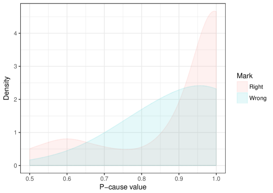
Figure 1: Density distribution of correct indications in relation to bootstrap ”p-cause” values.

We analyzed the accuracies of the causal paths discoveries for the best combination of algorithms and for those pairs for which ”p-cause” was at least 0.9 (70 pairs; approximately $73\%$ of all results), and obtained an accuracy of about $83\%$, which is greater than that obtained without analyzing ”p-cause”. Interestingly, taking into account only those pairs for which ”p-cause”$=1$ does not increase the accuracy further, but only reduces the number of pairs included in the analysis (59 pairs; $62\%$). Taking only those cases where all methods produced the same result (unanimity; $55.8\%$ of results) actually reduces the accuracy. All statistics are provided in Table 3.

Table 3: The summary of the accuracies of the causal path discoveries for the best combination, obtained for sets restricted with various criteria to increase the level of certainty.

Combination	Accuracy	Sensitivity	Specificity	Cohen’s Kappa
M2 + M3 + M4 (p>0.9)	0.8286	0.9020	0.6316	0.5518
M2 + M3 + M4 (p=1)	0.8136	0.9024	0.6111	0.5387
M2 + M3 + M4 (unanimity)	0.7358	0.7500	0.7143	0.4568

The strength of the unanimity measure combined with the ”p-cause” parameter was assessed. A boxplot comparing the distribution of ”p-cause” values is presented in Figure 2. The results showed that the median value equals 1 for both cases. However, for ”unanimity” cases, $75\%$ of results exceed 0.9, the level we chose to declare sensible causal path, which strengthens the inference possibilities.

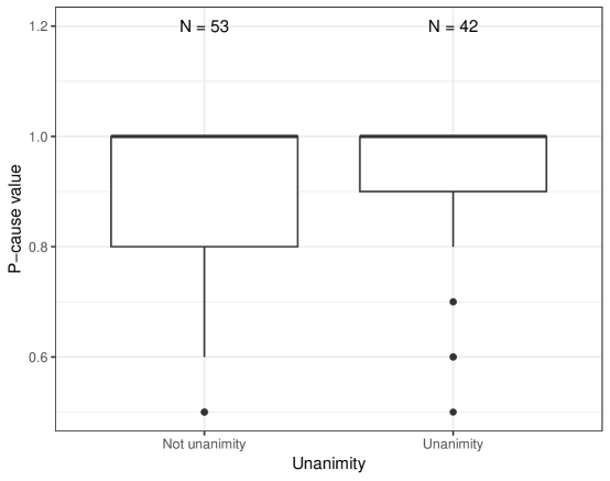
Figure 2: Distribution of ”p-cause” in relation to unanimity of all three methods.

Then, we analyzed (results in Table 4) the accuracy of causal path discovery for two sets of cases, with:

• significant Pearson’s correlation coefficients - $94.7\%$ pairs; interestingly, for all 4 pairs with insignificant correlation coefficients, the outcomes were correct;

• significant Bayesian correlation coefficients - $95.8\%$ pairs; the remaining 2 pairs with insignificant correlation coefficient also had correct results.

Table 4: The summary of the accuracies of the causal path discoveries for the best combination, after removing cases with insignificant correlation coefficients. PC crit. - the absolute value of Pearson’s correlation coefficient is statistically significant and greater then $0.1$; BC crit. - the absolute value of the Bayesian correlation coefficient is statistically significant ($MFE>0.9$) and greater then $0.1$.

Combination	Accuracy	Sensitivity	Specificity	Cohen’s Kappa
M2 + M3 + M4 (PC crit.)	0.7889	0.8750	0.5769	0.4680
M2 + M3 + M4 (BC crit.)	0.7912	0.8769	0.5769	0.4701

The curves of balanced accuracy (the mean of sensitivity and specificity), overall accuracy and Cohen’s Kappa, in relation to the number of observations in the considered cases, are presented in Figures 3-5, respectively.

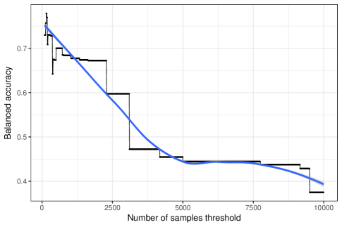
Figure 3: Distribution of balanced accuracy in relation to the number of observations; the blue line represents the local polynomial regression fitting function.

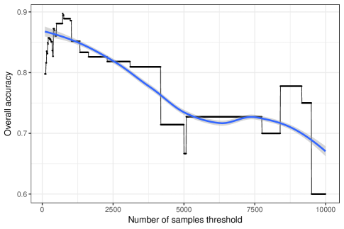
Figure 4: Distribution of overall accuracy in relation to the number of observations; the blue line represents the local polynomial regression fitting function.

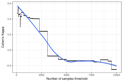
Figure 5: Distribution of Cohen’s Kappa in relation to the number of observations; the blue line represents the local polynomial regression fitting function.

It appears that a small number of observations does not impact the accuracy; one might even say that a low number provides better accuracy. The maximum for balanced accuracy and Cohen’s Kappa was found at 154, and at 724 for overall accuracy.

4 Discussion

In this paper, presented the results of a test of several methods intended for causal path discovery without prior knowledge of the data pairs coming from different fields of research. The best accuracy was obtained for the combination of generalized correlations framework, kernel regression absolute residuals criteria (AR) and causal additive modeling (CAM). All results were provided for the entire dataset cases; we did not have to divide the data into a training and test set (like in supervised learning approaches) because the analysis for each pair was treated as an independent step.

Several other methods could be included here based on meeting the basic criteria. For instance, mediation analysis and its extensions seem promising. However, it is relevant to problems of three or more variables, whereas the presented benchmark focused on the most elementary connections, within pairs. Still, the results from the analyzed framework could also serve as the input consideration for mediation analysis.

Otherwise, as in the case of the machine learning approach, we are not directly dependent on the training data, as well as on the consistency of the subsequent data used for testing and validation.

In the contest report, it is stated that several baseline methods were utilized, e.g., additive-noise, latent variable or complexity-based models, as well as machine learning methods. Various aspects were evaluated, e.g., dependency, confounding, causality and final score. However, in order to compare them with the metrics used in this study, only causality seems relevant. Interestingly, such approaches gave slightly worse results, with about $76\%$ accuracy for real data as the best result. Several issues were also surveyed, e.g., preprocessing, feature extraction, dimensionality reduction, classification and time spent; this seems far more sophisticated than the approach presented in the benchmark study [Guyon (2014)].

The presented approach demonstrates the possibility of establishing causal paths’ direction based only on the data. We assume that this approach, when combined with information from experts, may enable universal assessment of causality. It seems impossible to choose real causal explanations only by looking at observed data: such prior knowledge would allow acquisition of causal information without performing interventions. In the study, the context is different. We believe that for causal analysis, especially in data cases for which bidirectional links are assumed as well as for small data sets, the results cannot be very dependent on prior knowledge, but they can complement it generally.

On the other hand, it seems that the presented approach could complement time-series analyses based on newer approaches and generalizations of Granger causality [Porta and Faes (2016)]. We plan to connect such approaches and would also like to analyze the impact of many parameters, which can be established through the CAM process.

4.1 Limitations

In the presented study, we did not analyze the distribution of data in each case, nor the cross-associations between pairs. This is because the data comes from various fields and such processing could not be coherent with the main objective. Still, the impact of mentioned aspects should be addressed.

We wanted to focus on assessing elementary connections; as for the practical applications, the causal path for a set of more than two variables can be also established using the presented combination of methods, though this was not analyzed.

Also, it turned out that it is reasonable to determine the direction of a relationship only for data that fulfills the bootstrap simulation criterion (”p-cause”$>=0.9$); some results will be questioned, although their proportion seems sensible. Admittedly, as ”p-cause” comes from bootstrap simulation, its value is not very stable, so the proposed criterion should be viewed as as merely informative, not explicit.

5 Conclusion

In this benchmark study, an analysis of the accuracy of determining causal paths from the data from a causality contest was presented with the premise that the ground truth information is not taken into account for the discovery. The best overall accuracy was achieved for a combination of three methods: generalized correlations framework, kernel regression absolute residuals criteria (AR) and causal additive modeling (CAM). The most similar sensitivity and specificity values were obtained for AR criterion.

We proposed to establish the causal path for about $73\%$ of the considered pairs based on the ”p-cause” criterion; the remaining cases are proposed to be left as indeterminate. The correlation coefficients and number of observations seemed to not affect the result much.

In our opinion, the described approach can be used for preliminary dependence assessment, as an initial step for the commonly used causality assessment methods, or for comparison of data-driven findings with the ground truth.

SUPPLEMENTARY MATERIAL

T1:

The list of pairs from the database that were taken into consideration in the presented benchmark study [Mooij et al. (2016); Dheeru and Karra Taniskidou (2017)]. The ground truth column stores the path of cause and effect; abbreviation: UCI - from UCI Machine Learning Repository.

No.	Description	Ground truth (Path)
1	Deutscher Wetterdienst Data	Altitude $\rightarrow$ Temperature
2	Deutscher Wetterdienst Data	Altitude $\rightarrow$ Precipitation
3	Deutscher Wetterdienst Data	Longitude $\rightarrow$ Temperature
4	Deutscher Wetterdienst Data	Altitude $\rightarrow$ Sunshine
5	Abalone data (UCI)	Rings $\rightarrow$ Length
6	Abalone data (UCI)	Rings $\rightarrow$ Shell Weight
7	Abalone data (UCI)	Rings $\rightarrow$ Diameter
8	Abalone data (UCI)	Rings $\rightarrow$ Height
9	Abalone data (UCI)	Rings $\rightarrow$ Whole Weight
10	Abalone data (UCI)	Rings $\rightarrow$ Shucked Weight
11	Abalone data (UCI)	Rings $\rightarrow$ Viscera Weight
12	Census Income KDD (UCI)	Age $\rightarrow$ Wage per hour
13	Auto-Mpg Data (UCI)	Displacement $\rightarrow$ MPG
14	Auto-Mpg Data (UCI)	MPG $\rightarrow$ Horse power
15	Auto-Mpg Data (UCI)	Weight $\rightarrow$ MPG
16	Auto-Mpg Data (UCI)	Horse power $\rightarrow$ Acceleration
17	Census Income KDD (UCI)	Age $\rightarrow$ Dividends from stock
18	Concentration of GG versus age for pediatrician	Age $\rightarrow$ GAG concentration
19	Old Faithful geyser data	Duration of eruption $\rightarrow$ Time to the next eruption
20	Deutscher Wetterdienst Data	Latitude $\rightarrow$ Temperature
21	Deutscher Wetterdienst Data	Longitude $\rightarrow$ Precipitation
22	Cardiac Arrhythmia Database (UCI)	Age $\rightarrow$ Height
23	Cardiac Arrhythmia Database (UCI)	Age $\rightarrow$ Weight
24	Cardiac Arrhythmia Database (UCI)	Age $\rightarrow$ Heart Rate
25	Concrete Compressive Strength	Cement $\rightarrow$ Compressive Strength
26	Concrete Compressive Strength	Blast furnace slag $\rightarrow$ Compressive Strength
27	Concrete Compressive Strength	Fly Ash $\rightarrow$ Compressive Strength
28	Concrete Compressive Strength	Water $\rightarrow$ Compressive Strength
29	Concrete Compressive Strength	Superplasticizer $\rightarrow$ Compressive Strength
30	Concrete Compressive Strength	Coarse Aggregate $\rightarrow$ Compressive Strength
31	Concrete Compressive Strength	Fine Aggregate $\rightarrow$ Compressive Strength
32	Concrete Compressive Strength	Age $\rightarrow$ Compressive Strength
33	BUPA liver disorders (UCI)	Drinks $\rightarrow$ Mean Corpuscular Volume
34	BUPA liver disorders (UCI)	Drinks $\rightarrow$ Alkaline Phosphotase
35	BUPA liver disorders (UCI)	Drinks $\rightarrow$ Alanine Aminotransferase
36	BUPA liver disorders (UCI)	Drinks $\rightarrow$ Aspartate Aminotransferase
37	BUPA liver disorders (UCI)	Drinks $\rightarrow$ Gamma-glutamyl Transpeptdase
38	Pima Indians Diabetes Database	Age $\rightarrow$ BMI
39	Pima Indians Diabetes Database	Age $\rightarrow$ 2-Hour serum insulin
40	Pima Indians Diabetes Database	Age $\rightarrow$ Diastolic Blood Pressure
41	Pima Indians Diabetes Database	Age $\rightarrow$ Plasma glucose concentration a 2 hours in an oral glucose tolerance test
42	Private archive of Bernward Janzing	Days of the year $\rightarrow$ Mean Daily Temperature of Furtwangen
43	Mean Daily Air temperature near surface	Day 50 $\rightarrow$ Day 51
44	Mean Daily pressure at surface	Day 50 $\rightarrow$ Day 51
45	Mean daily sea level pressure	Day 50 $\rightarrow$ Day 51
46	Mean daily relative humidity near surface	Day 50 $\rightarrow$ Day 51
48	Time series modelling of water resources and environmental systems	Outdoor temperature $\rightarrow$ Indoor temperature
49	Daily mean values of ozone and temperature of year 2009 in Lausanne-César-Roux	Temperature $\rightarrow$ Ozone
50	Daily mean values of ozone and temperature of year 2009 in Chaumont	Temperature $\rightarrow$ Ozone
51	Daily mean values of ozone and temperature of year 2009 in Davos-See	Temperature $\rightarrow$ Ozone
56	UNdata from data.un.org	Latitude of the Country’s Capital $\rightarrow$ Fife Expectancy at Birth for female (2000-2005)
57	UNdata from data.un.org	Latitude of the Country’s Capital $\rightarrow$ Fife Expectancy at Birth for female (1995-2000)
58	UNdata from data.un.org	Latitude of the Country’s Capital $\rightarrow$ Fife Expectancy at Birth for female (1990-1995)
59	UNdata from data.un.org	Latitude of the Country’s Capital $\rightarrow$ Fife Expectancy at Birth for female (1985-1990)
60	UNdata from data.un.org	Latitude of the Country’s Capital $\rightarrow$ Fife Expectancy at Birth for male (2000-2005)
61	UNdata from data.un.org	Latitude of the Country’s Capital $\rightarrow$ Fife Expectancy at Birth for male (1995-2000)
62	UNdata from data.un.org	Latitude of the Country’s Capital $\rightarrow$ Fife Expectancy at Birth for male (1990-1995)
63	UNdata from data.un.org	Latitude of the Country’s Capital $\rightarrow$ Fife Expectancy at Birth for male (1985-1990)
64	UNdata from data.un.org	Population with sustainable access to improved drinking water sources $\rightarrow$ Infant mortality rate
65	Financial data from Jan. 4, 2000 to Jun. 17, 2005	Stock returns of Hang Seng Bank $\rightarrow$ Stock return of HSBC Hldgs
66	Financial data from Jan. 4, 2000 to Jun. 17, 2005	Stock returns of Hutchison $\rightarrow$ Stock return of Cheung kong
67	Financial data from Jan. 4, 2000 to Jun. 17, 2005	Stock returns of Cheung kong $\rightarrow$ Stock return of Sun Hung Kai Prop.
68	Internet connections and traffic at the MPI for Intelligent Systems	Open HTTP Connections $\rightarrow$ Bytes Sent
69	Temperature data provided by Joris M. Mooij	Outdoor temperature $\rightarrow$ Indoor temperature
72	Sunspot data	Sunspot Area $\rightarrow$ Global Mean Temperature Anomalies
73	Energy - emission data from 152 countries between 1960 and 2005	Energy use $\rightarrow$ CO2 emissions
74	UNdata from data.un.org	Gross National Income $\rightarrow$ Life Expectancy at Birth
75	UNdata from data.un.org	Gross National Income $\rightarrow$ Under 5 Mortality Rate
76	Data for 174 countries provided by Food and Agriculture Organization of the United Nations	Average Annual Rate of Change of Population $\rightarrow$ Average Annual Rate of Change of Total Dietary Consumption for Total Population
77	Data from 1985 to 2008, provided by Bernward Janzing	Solar Radiation measured in Furtwangen $\rightarrow$ Daily Average Temperature
78	Light Response Data	Photosynthetic Photon Flux Density $\rightarrow$ Net Ecosystem Productivity
79	Light Response Data	Photosynthetic Photon Flux Density, diffusive $\rightarrow$ Net Ecosystem Productivity
80	Light Response Data	Photosynthetic Photon Flux Density, direct $\rightarrow$ Net Ecosystem Productivity
84	Data for 3102 counties in US in 1980	Natural Logarithm of the Corresponding Population $\rightarrow$ Natural Logarithm of Employment
85	Milk protein trial data used by Verbyla and Cullis (1990)	Time to Take Weekly Measurements (from 1 to 14) $\rightarrow$ Protein Content of the Milk Produced by each Cow
87	Whistler Daily Snowfall	Mean Temperature $\rightarrow$ Total Snow
88	”bone” data set from CRAN	Age $\rightarrow$ Relative Spinal Bone Mineral Density
89	Data taken from Solly et al. (2014) on decomposition rates in forests and grasslands	Mass Loss in forests after 6 months $\rightarrow$ Mass Loss in forests after 1 year
90	Data taken from Solly et al. (2014) on decomposition rates in forests and grasslands	Mass Loss in grasslands after 6 months $\rightarrow$ Mass Loss in grasslands after 1 year
91	Data taken from Solly et al. (2014) on decomposition rates in forests and grasslands	Clay content in soil $\rightarrow$ Soil moisture at 10cm depth
92	Data taken from Solly et al. (2014) on decomposition rates in forests and grasslands	Clay content in soil $\rightarrow$ Organic C Content in Soil
93	MOPEX data set over 1948 to 2004	Average Precipitation $\rightarrow$ average Runoff
94	Data from a regional energy distributor in Turkey	Hour of the day $\rightarrow$ Temperature
95	Data from a regional energy distributor in Turkey	Hour of the day $\rightarrow$ Total Electricity Consumption
96	Data from a regional energy distributor in Turkey	Temperature $\rightarrow$ Total Electricity Consumption
97	Data on speed of a ball on a ball track for children, recorded by Dominik Janzing	Initial speed $\rightarrow$ Speed at later position
98	Data on speed of a ball on a ball track for children, recorded by Dominik Janzing	Initial speed $\rightarrow$ Final speed
99	’nlschools’ from the R MASS package	Social-Economic Status of Pupil’s Family $\rightarrow$ Language Test Score
100	’cpus’ from the R MASS package	Cycle time $\rightarrow$ Published performance on a benchmark mix
101	Brightness of screen	Grey value of a pixel $\rightarrow$ Light intensity seen by a photo diode
102	Data on speed of a ball, recorded by Dominik Janzing	Position on the ball track where the ball starts $\rightarrow$ Time interval between passing the first and the second light barrier
103	Data on speed of a ball, recorded by Dominik Janzing	Position on the ball track where the ball starts $\rightarrow$ Time interval between passing the third and the fourth light barrier
104	Data on speed of a ball, recorded by Dominik Janzing	Time interval between passing the first and the second light barrier $\rightarrow$ Time interval between passing the third and the fourth light barrier
106	Speed of an electric toy locomotive	Electric voltage $\rightarrow$ Time required for passing one round
108	Data on heat bath of a Striling engine	Temperature $\rightarrow$ Time for 1/6 rotation

References

- Bühlmann et al. (2014) Bühlmann, P., J. Peters, J. Ernest, et al. (2014). Cam: Causal additive models, high-dimensional order search and penalized regression. The Annals of Statistics 42(6), 2526–2556.
- Chen et al. (2004) Chen, Y., G. Rangarajan, J. Feng, and M. Ding (2004). Analyzing multiple nonlinear time series with extended granger causality. Physics Letters A 324(1), 26–35.
- Chickering (2002) Chickering, D. M. (2002). Optimal structure identification with greedy search. Journal of machine learning research 3(Nov), 507–554.
- Dheeru and Karra Taniskidou (2017) Dheeru, D. and E. Karra Taniskidou (2017). UCI machine learning repository. http://archive.ics.uci.edu/ml.
- Granger (1969) Granger, C. W. (1969). Investigating causal relations by econometric models and cross-spectral methods. Econometrica: Journal of the Econometric Society, 424–438.
- Guyon (2014) Guyon, I. (2014). Results and analysis of the 2013 chalearn cause-effect pair challenge. In Proceedings of NIPS 2013 Workshop on Causality: Large-scale Experiment Design and Inference of Causal Mechanisms.
- Kaggle (2013) Kaggle (2013). Cause-effect pairs. https://www.kaggle.com/c/cause-effect-pairs. [Online; accessed 27-June-2018].
- Mooij et al. (2016) Mooij, J. M., J. Peters, D. Janzing, J. Zscheischler, and B. Schölkopf (2016). Distinguishing cause from effect using observational data: methods and benchmarks. The Journal of Machine Learning Research 17(1), 1103–1204.
- Neyman (1923) Neyman, J. (1923). Sur les applications de la théorie des probabilités aux experiences agricoles: Essai des principes. Roczniki Nauk Rolniczych 10, 1–51.
- Pearl (1995) Pearl, J. (1995). Causal diagrams for empirical research. Biometrika 82(4), 669–688.
- Pearl (2009) Pearl, J. (2009). Causality: Models, Reasoning and Inference. Cambridge University Press.
- Pearl (2010) Pearl, J. (2010). The foundations of causal inference. Sociological Methodology 40(1), 75–149.
- Pearl et al. (2009) Pearl, J. et al. (2009). Causal inference in statistics: An overview. Statistics surveys 3, 96–146.
- Peters and Ernest (2015) Peters, J. and J. Ernest (2015). CAM: Causal Additive Model (CAM). R package version 1.0.
- Porta and Faes (2016) Porta, A. and L. Faes (2016). Wiener–granger causality in network physiology with applications to cardiovascular control and neuroscience. Proceedings of the IEEE 104(2), 282–309.
- R Core Team (2018) R Core Team (2018). R: A Language and Environment for Statistical Computing. Vienna, Austria: R Foundation for Statistical Computing.
- Rebane and Pearl (2013) Rebane, G. and J. Pearl (2013). The recovery of causal poly-trees from statistical data. arXiv preprint arXiv:1304.2736.
- Rubin (1974) Rubin, D. B. (1974). Estimating causal effects of treatments in randomized and nonrandomized studies. Journal of educational Psychology 66(5), 688.
- Rubin (2005) Rubin, D. B. (2005). Causal inference using potential outcomes: Design, modeling, decisions. Journal of the American Statistical Association 100(469), 322–331.
- Schölkopf et al. (2012) Schölkopf, B., D. Janzing, J. Peters, E. Sgouritsa, K. Zhang, and J. Mooij (2012). On causal and anticausal learning. arXiv preprint arXiv:1206.6471.
- Spirtes (2010) Spirtes, P. (2010). Introduction to causal inference. Journal of Machine Learning Research 11(May), 1643–1662.
- Spirtes et al. (2000) Spirtes, P., C. N. Glymour, R. Scheines, D. Heckerman, C. Meek, G. Cooper, and T. Richardson (2000). Causation, prediction, and search. MIT press.
- Vinod (2017) Vinod, H. D. (2017). Generalized correlation and kernel causality with applications in development economics. Communications in Statistics-Simulation and Computation 46(6), 4513–4534.
- Vinod et al. (2018) Vinod, P. H. D., F. University, and NY. (2018). generalCorr: Generalized Correlations and Initial Causal Path. R package version 1.1.1.
- Zhang (2006) Zhang, J. (2006). Causal inference and reasoning in causally insufficient systems. Ph. D. thesis, PhD thesis, Carnegie Mellon University.
- Zhang et al. (2017) Zhang, K., B. Schölkopf, P. Spirtes, and C. Glymour (2017). Learning causality and causality-related learning: some recent progress. National Science Review.
- Zheng et al. (2012) Zheng, S., N.-Z. Shi, and Z. Zhang (2012). Generalized measures of correlation for asymmetry, nonlinearity, and beyond. Journal of the American Statistical Association 107(499), 1239–1252.