AK-type stability theorems on cross -intersecting families
Sang June Lee
Department of Mathematics, Kyung Hee University, Seoul 02447, South Korea
sjlee242@khu.ac.kr, Mark Siggers
College of Natural Sciences, Kyungpook National University, Daegu 702-701, South Korea
mhsiggers@knu.ac.kr and Norihide Tokushige
College of Education, Ryukyu University, Nishihara, Okinawa 903-0213, Japan
hide@edu.u-ryukyu.ac.jp
Abstract.
Two families, and , of subsets of are
cross -intersecting if for every and ,
and intersect in at least elements.
For a real number and a family the product measure
is defined as the sum of over all
.
For every non-negative integer , and for large enough , we determine, for any satisfying
, the maximum possible value of
for cross -intersecting families and .
In this paper we prove a stronger stability result which yields the
above result.
Key words and phrases:
Cross intersecting families; Erdős-Ko-Rado theorem; Ahlswede-Khachatrian theorem; Shifting; Random walks
The first author was supported by Korea Electric Power Corporation (Grant number:R18XA01) and by Basic Science Research Program through the National Research Foundation of Korea (NRF) funded by the Ministry of Education (NRF-2016R1D1A1B03933404 and NRF-2019R1F1A1058860). The second author is supported by Korean NRF Basic Science Research Program (NRF-2018R1D1A1A09083741) and by the Kyungpook National University Research Fund. The last author was supported by JSPS KAKENHI 25287031, 18K03399
1. Introduction
Let be positive integers. Let and
.
A family of subsets is called -intersecting
if for all .
For any real number and a family ,
we define the product measure of by
What is the maximum product measure of -intersecting families?
To answer this question, let be a non-negative integer and let
The family is -intersecting since
for all . Two families
are isomorphic, denoted by , if
, where is a permutation on .
Answering a conjecture of Frankl, and extending partial results by Frankl and Füredi in [12],
the following result is essentially proved in [1] by Ahlswede and
Khachatrian, see also [2, 6, 9, 16].
Theorem 1.
If is -intersecting, then
Moreover, equality holds if and only if for some .
Grouping the subsets in the family according to the size of
their intersection with we see, where ,
(1)
By comparing and
, one sees that
is positive, , negative
if and only if is positive, , negative, respectively.
In particular, if
(2)
then
Thus the Ahlswede–Khachatrian theorem says that the maximum product measure
of -intersecting families is given by provided that and satisfy (2).
We extend this result to two families in . Two families
are cross -intersecting if
for all and .
In this case, it is conjectured in [15] that
(3)
under the assumption of
(2). The inequality (3) was proved for and in [13] and for and in [15]. We also mention that Borg obtained related results in
[3, 4, 5].
In this paper, using the random-walk method that was introduced by Frankl in [10, 11], we verify
that this conjecture holds for every fixed and large .
That is we prove the following, referring to [13] for the case .
Theorem 2.
For every integer , there exists an integer , depending only on ,
such that for all and all with
, the following
holds.
If are cross -intersecting, then
(4)
Moreover, equality holds if and only if one of the following holds:
(i)
and ,
(ii)
and , or
(iii)
and .
In this paper we do not attempt to optimize .
We simplify calculations by assuming, for each fixed , that is sufficiently large.
As such, when we use asymptotic notation such
as , , or , it is always asymptotic in , with fixed,
and being some fixed proportion of the way through the range (2).
We also consider the stability of extremal structures. Suppose that
are cross -intersecting families.
If condition (2) is satisfied and
is close to the maximum value, then we can ask whether and are
close to (isomorphic copies of) the extremal families ,
or , where we say that two families and are close
if their symmetric difference
has small measure.
We are able to show that this is true if the
two families satisfy the additional condition of being ‘shifted.’
A family is shifted (sometimes called compressed)
if and
for some imply
.
It is known (see, e.g., Lemma 2.3 in [13]) that for any given
cross -intersecting families one can apply a
sequence of shifting operations to them and get shifted
cross -intersecting families such that
and .
Notice that the definition of a shifted family depends on the ordering
of , so an isomorphic copy of a shifted family is not
necessarily shifted in this sense.
A family is inclusion maximal if and
imply as well. Since we are interested in the maximum measure of cross -intersecting families, we always assume that families are inclusion maximal.
It is not difficult to see that the property of
being inclusion maximal is invariant under shifting operations.
Two families and are -nice if they are shifted,
inclusion maximal, and cross -intersecting.
We obtain the following statement of stability.
Theorem 3.
For every integer and all real numbers and , there exists an integer such that
for all
the following holds.
Let
, and let be -nice families.
If
(5)
with
, then
(6)
For , a similar result was proved in [13]; for the same it is weaker than this, but it is proved for .
There are some points about this theorem that bear further explanation.
For one, no matter how close we require that
be to in (5) there are -nice
families and , which are not
subfamilies of , that satisfy (6).
Indeed, consider the families
The families and are -nice, and
for as .
Theorem 3 says that such families and must be close to in the sense that the sum of their measures
goes to .
Observe that with such a definition of closeness, inequality (6) is sharp.
Indeed, if and
then the LHS of (6)
is precisely .
Another point we should explain is the reduced range of in the statement of the theorem.
When we have , so to make a statement of
stability with respect to it is necessary to move away from this point. We thus introduce
a gap of into the bound , and once this is introduced, we
absorb constants into it and simplify it to .
Similarly, we require because of the family .
As goes to , we must introduce in (5) that depends on .
It turns out that the condition is sharp.
Indeed, consider the following pair of families:
and .
The families and are -nice, and far from ,
in fact, both
and
go to infinity as .
On the other hand, one
can show that if , then
For a full stability result, we must consider these other extremal
families. We do this with the more complicated
Theorem 4,
from which Theorem 3 follows as a corollary.
Assume that and are -nice families,
and (2) is satisfied.
Theorem 4 says that
either is much smaller than the optimal value , or is close to one of
, ,
, ,
or .
(7)
We denote the set of pairs of subscripts of the extremal families in (7)
by
(8)
If is close to optimal, then we will have, up to switching and ,
that is close to for a unique , with
and . Again, to quantify ‘close to’ we consider the measure
of the symmetric differences
and . We could just sum these, but we will
observe below, in (20), that , so the measures of
and can be vastly different. It is natural,
therefore, to normalise the measures of these symmetric differences with respect to the measures of
and .
We thus define the following normalised measures:
Now we can state our main result.
Theorem 4.
For every integer , and all real numbers
, and ,
there exists an integer
such that for all the following holds. Let
and let be
-nice families.
Suppose
(9)
Then, up to switching and , there exists unique such that, for
the following hold.
(a)
with equality holding if and only if
and ,
(b)
, and
(c)
with equality holding if and only if
and .
What does this say exactly? It says that if the product of the measures of
and is close to optimal, then has measure not greater than one of the
one of the pairs of extremal families in (7), and is
close to this pair, in the sense that is small.
To see that is small one can use (b) to show
as we do for (15).
That the measure of is at most that of is stated with (a) and (c).
We explain why there are two statements. The statements are very similar when
(9) holds. Statement (c) is perhaps the more obvious statement, in light of
the required inequality (4) of Theorem 2, and in the case that
it is all we need for proving both Theorem 2 and
3. Moreover, in this
case (c) follows from (a) by the AM-GM inequality. When things are not so clean, and
we need both statements. Statement (a) is stronger as approaches or
and so we use this to prove Theorem 2. When is bounded away from these
endpoints, (c) is stronger (and harder to prove) than statement (a). We use it to
prove Theorem 3.
We mention that the inequality in (a) is not necessarily true
unless (9) holds. Indeed if, e.g.,
,
or , then it follows that
if .
We also mention that the condition is tight.
To see this, let ,
or , and let .
Then and are -nice, and we have ,
(and the LHS converges to the RHS as ,) but (b) does not hold for
any .
This means that one cannot replace the condition (9) with
.
The organization of this paper is as follows.
In Section 2 we
derive Theorems 2 and 3 from
Theorem 4. Most of the rest of the paper is dedicated to the proof of
Theorem 4.
In Section 3 we recall some useful tools from [13] and [15].
In Section 4.1 we lay out our asymptotic assumptions
and use them to give simplified expressions for frequently used values.
In Section 4.2
we reduce Theorem 4 to the
essential case: . We then define the parameters and ,
and use them to distinguish three cases for the proof of
Theorem 4: the non-extremal case, the diagonal extremal case, and the non-diagonal extremal case.
In Section 5 we settle the non-extremal case.
We deal with the diagonal extremal case in
Section 6, and then, following the proof of this very closely,
we consider the non-diagonal extremal case in Section 7.
In Section 8 we make some brief comments about a recent result of
Ellis, Keller and Lifshitz [8] which is related to Theorem 3.
The case of Theorem 2 is proved in [13], and hence, we fix .
Let be a fixed constant in , and let
be of Theorem 4.
Let be chosen so that
and .
We first suppose that are -nice families.
If condition (9) of Theorem 4 does
not hold, then Theorem 2 is clearly true, so assume
it holds and apply Theorem 4. This gives us
values .
In the case that , we have . Item (c) of
Theorem 4 gives
where the equality holds if and only if
and satisfy one of (i), (ii), and (iii) of
Theorem 2.
In case that , the AM-GM inequality and (a) of
Theorem 4
imply that
Except for proving this claim, we have thus proved Theorem 2 provided that
and are -nice families.
Now suppose that and are
(not necessarily shifted) inclusion maximal and cross -intersecting
families. Let and be -nice families obtained
from and after applying a sequence of shifting operations.
Then, by the fact we have just proved, the families and
satisfy the inequality (4) with the equality conditions.
Since the measure is invariant under shifting operations, we have , and hence,
we still have (4) for and . Moreover, it is known
from Lemma 6 in [15] that if then
. Thus the equality conditions hold for and
as well. This completes the proof of Theorem 2, up to the
proof of Claim 1, which we give now.
First, we consider the case where .
Using , it follows from (1) (see also (19)) that
(10)
Hence, we can check Claim 1 by comparing the main terms of
and . That is, it suffices to show
,
that is,
,
or equivalently,
.
The LHS is minimized, for satisfying (2), at
; and in this case the above
inequality is equivalent to .
Next, we consider the case where . In this case it suffices to show that
,
or equivalently,
.
The LHS is maximized at and then the above
inequality is equivalent to .
∎
Although we use [13] for the case , we could have proved this case with
Theorem 4 as well; but it would have required a slightly more complicated statement.
The only problem in applying Theorem 4 as is, is the condition
in the case . This condition is used only in proving Lemma 18, which gives us
item (c) of Theorem 4 in the case that .
However, we only need (a) of Theorem 4 to prove Theorem 2.
Let , and be given, and set so that
,
(which implies ).
Let , and
for
or for
be determined by Theorem 4.
Let and be families, as in the setup of Theorem 3, that satisfy (5).
Then (9) holds, and we can apply
Theorem 4 to get for which
(a)–(c) hold.
We consider the following three cases separately:
Case 1 or ,
Case 2 or ,
Case 3 .
Case 1. Since , we have
and .
By (c) of Theorem 4, we have
(11)
Claim 2.
Let and .
If , then
(12)
Proof.
Recall that and .
First, let .
Note that .
Using (10), and in the last inequality that , we get
Next, for the case one can similarly check that
Combining (11) and (12)
contradicts (5), and hence Case 1 cannot happen.
This proves (6), and completes the proof of Theorem 3.
3. Preliminary tools
3.1. Walks corresponding to subsets
It is useful to regard a set as an -step walk starting at the
origin of the two-dimensional grid as follows.
If , then the -th step is up from to .
Otherwise, the -th step is right from to .
From now on, we refer to as a set or a walk.
Figure 1. Walk corresponding to
A walk reaches the point on the line
if and only if .
For an integer let
be the family of all walks that hit the line ,
where is defined in (1).
We further define
This gives a partition .
Let and
.
One can estimate the measure of the families defined above using random walks, and this is one of the main ideas for proving our results.
Consider an infinite random walk in the plane starting from the
origin, each step of which is a random variable, independent of other steps, going up with probability and right with probability
.
The product measure of the family of walks that satisfy some property is
the probability of a random walk satisfying that property.
Example 4.
Let be the family of all walks that hit the point for
integers and . There are different walks from
to , and a random walk is any one of these
with probability , so .
With a little more work, one can show that the infinite random walk
hits the line with probability precisely , where
. Based on this fact,
one can show the following.
The number of walks from to that do not hit the
line is .
3.2. Dual walks and some facts
For , let be the -th smallest element of .
For , we say that shifts to , denoted by
, if and for each .
As an example, we have .
Viewing and as walks, means that the walk is above
the walk on the grid .
The dual of with respect to is defined by
(16)
See Figure 4 for an example of a walk and its dual.
Note that . Furthermore, is the shift minimal
walk satisfying this condition, and hence, if then
. As walks, is obtained by
reflecting across the line and
replacing the part with the path connecting and
.
The following fact is immediate.
The rest of the paper is dedicated to the proof of Theorem 4.
4.1. Basic Asymptotics
In this section we talk about the assumptions we will use in asymptotic arguments.
From now on, we let be a fixed integer, and if then let also be fixed. Let
let be a sufficiently large integer depending on and .
Since we are interested in the maximum possible measure
over all -nice pairs , where ,
and this value is non-decreasing in (see Lemma 2.12 in [13]),
we may assume that is sufficiently large
compared to . Consequently, we assume that
First assume that ,
and satisfies
which gives
(17)
where goes to as .
This implies that
,
and using it follows that
;
in particular, . We also have that
Suppose now that and that . Then (18) and (20) trivially hold.
In particular,
holds for any pair in (7)
for , as well as in
, , and .
4.2. Initial reductions and definition of cases
In this section, we make initial reductions for the proof of
Theorem 4, and introduce parameters by which we can
break the remainder of the proof into cases.
We have already fixed . Let and
be given. We will choose , depending on these
constants, to be sufficiently large. Only matters in this and the next sections,
and then or will get involved in
Sections 6 and 7.
Choose .
Let be -nice families.
Where , for , is the maximum
such that , let
Without loss of generality, we may assume that .
Since and are -nice,
we have , see e.g., Lemma 2.11 of [13].
Since , we have a partition
, where
, , and
.
Similarly, we have a partition
.
Lemma 8.
If either , , or , then
.
Proof.
Suppose that . Lemma 5 yields that
and ,
so by (18) and (20) it follows
.
Next suppose that , then
Lemma 5 gives
, and thus
.
The same holds if .
∎
Lemma 8 guarantees the existence of depending on
and
such that if and and are -nice families satisfying (9),
then we necessarily have that , , and
.
Moreover, one can show the following.
Suppose that and . Then,
there exist unique non-negative integers and such that
and
.
Moreover, . In particular, .
Here, we record the main discussion of this and the previous section.
Setup.
For a proof of Theorem 4 we may assume the following.
•
is a fixed integer.
•
, and
are fixed real numbers.
•
.
( depends on , which will be described later.)
•
for , and for
.
•
and .
•
are -nice, that is, shifted,
inclusion maximal, and cross -intersecting.
•
, , ,
.
•
, , , .
•
,
,
, ,
,
.
Under this setup, the proof of Theorem 4 breaks down into three cases: Recalling defined in (8), we consider
NE: the non-extremal case ,
DE: the diagonal extremal case and ,
NDE: the non-diagonal extremal case and .
5. Non-extremal cases
In this section,
we deal with the case NE, that is, the case when . We prove the following lemma.
By choosing , depending on , sufficiently large,
the lemma shows that Theorem 4 holds vacuously for ,
since (9) does not hold.
Lemma 10.
If then
.
For a proof of Lemma 10, recall that .
Recall also that no walk in hits the line
while all walks in hit one of
.
Since all walks in
must hit .
Thus, by Example 4,
we have
This together with
, which we get from
Lemma 5, yields
where
(21)
Similarly we have .
Thus we have
Hence, in order to show Lemma 10, it suffices to show
(22)
5.1. The case when is large
In this subsection we show (22) for the case .
We start by bounding the terms in and using the following claim, which uses only elementary calculus.
Claim 11.
If , then we have
(i)
,
(ii)
,
(iii)
.
Proof.
(i) Using and , we get
.
(ii) We have
.
Using and the assumption ,
we have .
Also, we have .
Thus we get
.
(iii) If then the inequality is true. Let .
First observe
We consider now three cases, depending on .
•
If then
for . Thus .
•
If then , and hence,
.
•
Finally let . We divide into two parts
and .
For the first part we have
for . For the second part, the derivative gives that is maximized at
as .
Thus .
This completes the proof of (22), and thus, of
Lemma 10 for the case .
5.2. The case when is small
In this subsection we show (22) for the case . In this case, we take advantage of the fact that is much smaller than . Let us estimate defined in (21).
Using and
we have
Similarly, .
Combining these with
(cf. (19)), we have
Our proof of (24) is based on the following observation.
Claim 12.
Let .
There is depending on such that for the following holds.
(i)
for .
(ii)
for ,
(iii)
for .
Of course, and can never be negative, so when or we replace
in (ii) or (iii) with .
Proof.
(i) It follows from (23) that
if is large enough then
is equivalent to .
(ii)
Recall that . By comparing and ,
we have that
and if is large enough.
(iii)
Let . Then, by (23), we have that
if is large enough then is equivalent to
. Hence,
and .
Indeed, if , then .
On the other hand, if , then .
∎
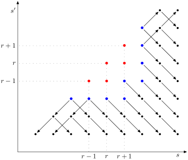
The arrows in Figure 2 illustrates the relation between the values
for values of and considered in Claim 12.
We mention that (24) does not hold for
, which is the reason that
we do not draw arrows starting from the points in .
The figure tells us that in order to show
(24) for it suffices to check
the following starting points when and are non-negative:
Figure 2. Relations on
The verification of (24) for these cases follows
from easy computation. For example,
as , and to mean this situation we write
. Similarly we have
Therefore, we get (24) for all ,
which completes the proof of Lemma 10 for the case .
In this section we deal with the case DE, that is, we assume that
or the latter two only, if .
Under the assumption we have that .
Defining the notation
,
we let
The parameter ranges over , where
is defined so that . Recalling the definition of the dual walk
in (16) on page 16, we have (see Figure 4)
Figure 3. Walks and
Figure 4. Walk
Consider the case where or .
By symmetry we may assume that .
In this case we show that Theorem 4 vacuously holds
since (9) does not hold.
Lemma 13.
If then , that is,
there exists depending on and such that
for all .
Proof.
First we show that
(25)
For the proof, let
.
Since , Fact 7 (i) gives that implies .
As and so we have
, and hence, .
Now, all walks in hit the line only at .
Hence, they necessarily hit and the -th step is ‘up’.
Using Fact 6 with , the number of ways for a walk in
to hit , and so , is .
Further, of such walks, those that hit are in , and this can happen in
ways. Therefore, looking at only the first steps, we
see that
Then we use
, and hence, we infer
.
Since ,
we have that
. On the other hand, (20) gives
.
Hence,
.
∎
Now we assume that both and contain .
Then we can define parameters as follows.
Since is shifted there exists with such that
for and for .
Similarly there is such that
for and for .
Based on their values, we consider the following two cases,
Case I: , and
Case II: Either or .
Case I.
In this case we apply the following to get .
Claim 14.
If , then . If , then .
Proof.
By symmetry, it is enough to prove only the first statement.
As , that is, , Fact 7 (ii) gives that
.
So Fact 7 (i) implies that each walk satisfies Note that which
consists of line segments connecting , , ,
and .
Thus each walk must hit one of ,
which means .
Hence, holds.
∎
One can easily check that Theorem 4 (a)–(c) follow from Claim 14. Note that the equality in (a) and (c) holds if and only if .
Case II. First we prove
(27)
that is, (b) of Theorem 4 holds for ,
where depends on and .
(Note that we do not assume (9) here.)
Since
and
,
it suffices to show that
(28)
By symmetry we only show (28).
If then by Claim 14
and (28) holds. So we may assume that ,
and there exists .
Claim 15.
We have
and
.
Proof.
To prove the first inequality,
consider walks such that and hits .
Since , we have
by Fact 7 (i).
Since contains line segments connecting
, , and
it follows that must hit and .
(See Figure 4.)
The number of walks from to is , then there is the unique walk passing , , and which hits .
So the measure of the family of all such walks is .
After hitting , to satisfy , walks
must not hit the line .
This happens with probability at least
because the measure of walks starting from which hit this line is
at most by (i) of Lemma 5.
Thus we obtain
(29)
Next, we prove the second inequality.
Since , we have that .
Referring to Figure 4, with , one sees that
the walk contains line segments connecting
, , , and ; and then from
the walk never hits the line .
Hence, by Fact 7, each walk must hit one of ,
or .
Note that all walks hitting one of these points are contained in
. Thus, each walk hits .
So by Lemma 5 (i) we have
(30)
which completes the proof of the claim.
∎
It follows from the claim that
,
which yields (28), and then (27). Therefore we have
and so we get (a) of Theorem 4 without equality.
Then (c) follows from (a) with the AM-GM inequality, that is,
.
7. Non-diagonal extremal cases
We now deal with the remaining non-diagonal extremal cases or . In these cases, we have
, and hence, , and .
The argument here is similar to that of Section 6, but it
is slightly complicated because of the asymmetry
of and .
This together with
yields .
For we use the obvious estimation .
Thus .
If then we have . Indeed,
with only obvious changes to the proof of
Lemma 13, we get that
where
,
and, using , we have that
(If then and .)
Thus follows from
.
Since we get
.
Consequently if or then
.
∎
Now we assume that both and contain .
We define the parameters
and
.
We again have the following two cases, that is,
Case I: , and
Case II: Either or .
Case I.
In this case we have
and .
We can argue as in the previous section.
The assumption implies that
, and hence,
Similarly implies
One can easily check that Theorem 4 (a)–(c) follow from and .
Case II.
First we prove
(31)
that is, (b) of Theorem 4 holds for ,
where depends on and .
To this end it suffices to show the following.
Claim 17.
We have and
.
Proof.
First, we show the first inequality. If then this is true
because and
follow from the argument in Case I. So assume that .
Changing to in the argument used to give (29)
yields
and changing to in the argument for (30) gives
.
Thus
showing the first inequality.
Next, we prove the second inequality. This is clearly true if .
So assume that .
We have
and walks which hit and shift to
belong to .
These walks must hit , then and then , and
after hitting they never hit the line . Thus
while as
implies, following the
argument for (30), that each walk in
hits . Together this gives
. So
which proves the second inequality.
∎
Next we check that (a) of Theorem 4 holds without equality.
Indeed it follows from (31) that
Let for , and let
be any fixed constant satisfying
for .
Claim 17 gives that and
. So
and hence,
.
Therefore, in order to show Lemma 18, it suffices to show that
(32)
If both and are non-negative, then we clearly
have (32).
If both of them are negative or , then . This implies , and hence, we also get
(32). Thus we may assume that
, and
by symmetry, .
Since we have and
.
Also we have
.
Consequently we have and
(33)
Since (32) is rewritten as
and we know that the LHS is negative,
in order to prove (32)
it suffices to show that the RHS is non-negative, that is,
If , then using , , ,
and noting that attains its minimum at ,
we get
Similarly, if , then , that is, , and
In both cases we have , and this together
with (33) yields (34) as needed.
∎
8. Concluding remarks
Recently, Ellis, Keller and Lifshitz [7] obtained a sharp stability result for
-intersecting families. The following is Theorem 1.10 of [7] with only minimal
changes of notation.
For any and any , there exists such that the following holds.
Let , and let . If is a -intersecting family such that
, then there exists a family isomorphic to
such that .
Their result is related to
Theorem 3 for the case .
To make a comparison easier we state a version of our
Theorem 3, which can be proved almost exactly as
Theorem 3 is proved.
Theorem 6.
For every integer and all real numbers
and , there exists an integer such that
for all
the following holds.
Let
.
If are -nice families such that
with , then
In particular, if then
implies
.
Their setup is different from ours and it seems that
neither result implies the other. We should note that their results
apply to all (not necessarily shifted) -intersecting families.
It would be very interesting to see whether one can use their technique to remove the
shiftedness condition from Theorem 4.
See also [7, 14] for related stability results for intersecting
families.
References
[1]
R. Ahlswede, L.H. Khachatrian.
The diametric theorem in Hamming spaces–optimal anticodes.
Adv. in Appl. Math. 20 (1998) 429–449.
https://doi.org/10.1006/aama.1998.0588
[2]
C. Bey, K. Engel.
Old and new results for the weighted -intersection problem via AK-methods.
Numbers, Information and Complexity, Althofer, Ingo,
Eds. et al., Dordrech, Kluwer Academic Publishers (2000) 45–74.
https://doi.org/10.1007/978-1-4757-6048-4_5
[3]
P. Borg.
The maximum product of sizes of cross-t-intersecting uniform families.
Australas. J. Combin., 60/1 (2014) 69-–78.
link
[4]
P. Borg.
The maximum product of weights of cross-intersecting families.
J. Lond. Math. Soc. 94/2 (2016) 993–1018.
https://doi.org/10.1112/jlms/jdw067
[5]
P. Borg,
The maximum product of sizes of cross-intersecting families.
Discrete Math. 340/9 (2017) 2307–2317.
https://arxiv.org/abs/1605.08752
[7]
D. Ellis, N. Keller, N. Lifshitz.
Stability versions of Erdős-Ko-Rado type theorems, via isoperimetry.https://arxiv.org/abs/1604.02160
[8]
D. Ellis, N. Keller, N. Lifshitz.
Stability for the Complete Intersection Theorem, and the Forbidden Intersection Problem of Erdős and Sós.https://arxiv.org/abs/1604.06135v4
[10]
P. Frankl.
The Erdős–Ko–Rado theorem is true for .
Combinatorics (Proc. Fifth Hungarian Colloq., Keszthey, 1 (1976), 365–375)
Colloq. math. Soc. János Bolyai, 18, North–Holland, 1978.
[11]
P. Frankl.
The shifting technique in extremal set theory.
Surveys in combinatorics (New Cross, 1987) 81–110, London Math. Soc. Lecture Note Ser. 123.
http://www.renyi.hu/~pfrankl/1987-4.pdf
[13]
P. Frankl, S. J. Lee, M. Siggers, N. Tokushige,
An Erdős–Ko–Rado theorem for cross -intersecting families.
J. Combin. Theory (A) 128 (2014) 207–249.
https://doi.org/10.1016/j.jcta.2014.08.006
[15]
S. J. Lee, M. Siggers, N. Tokushige,
Towards extending the Ahlswede–Khachatrian theorem to cross -intersecting families.
Discrete Appl. Math. 216 (2017) 627–645.
https://doi.org/10.1016/j.dam.2016.02.015