Cheeger inequalities for graph limits

Abstract.

We introduce notions of Cheeger constants for graphons and graphings. We prove Cheeger and Buser inequalities for these. On the way we prove co-area formulae for graphons and graphings.

1. Introduction

The Cheeger constant, introduced in Riemannian geometry by Cheeger [Che70] in the early 70’s measures the ‘most efficient’ way to cut a closed Riemannian manifold into two pieces, where efficiency is measured in terms of an isoperimetric constant. Cheeger [Che70] and Buser related this geometric quantity to a spectral quantity–the bottom of the spectrum of the Laplacian. These are the well-known Cheeger-Buser inequalities in Riemannian geometry (see [Bus10, Section 8.3] for details). A discrete version of the Cheeger constant and the Cheeger-Buser inequalities was then obtained independently by Dodziuk [Dod84] and Alon-Milman [Alo86, AM85] for finite graphs (see [Chu10] for a number of different proofs and [Moh91] for a survey). These ideas and inequalities have also been extended to weighted graphs [FN02] (see also [Chu97, Chapter 2, pg. 24], [Tre11]). In a certain sense, this marked a fertile way of discretizing a notion that arose in the setup of continuous geometry.

More recently, the theory of graph limits, graphons and graphings was developed by Lovasz [Lov12] and others (see especially [BCL⁺08, BCL⁺12, BCKL13, Cha17]) giving a method of obtaining measured continua from infinite sequences of finite graphs. From a certain point of view, this gives us a path in the opposite direction: from the discrete to the continuous.

Such continuous limits come in two flavors: dense graphs (graphons) or sparse graphs (graphings). A graphon is relatively easy to describe: it is a bounded (Lebesgue) measurable function $W:I^{2}\to I$ that is symmetric: $W(x,y)=W(y,x)$ for all $x,y\in I$. A graphing on the other hand may be thought of as a measure on $I^{2}$ that can be locally described as a product of a sub-probability measure on $I$ with the counting measure on a set of uniformly bounded cardinality (see Sections 2.1 and 2.2 for details). Each of the co-ordinate intervals $I\times\{0\}$ and $\{0\}\times I$ may be thought of as the vertex set of the graphon or graphing and is equipped with a Borel measure.

The aim of this paper is to define the notion of a Cheeger constant for graphons and graphings and prove the Cheeger-Buser inequalities for them. For both a graphon $W$ and a graphing $G$, the Cheeger constants $h_{W}$ and $h_{G}$ respectively measure (as in Cheeger’s original definition) the best way to partition the “vertex set” $I$ into $A,A^{c}$ such that the isoperimetric constant is minimized. For instance for a graphon $W$,

(1.1) $$h_{W}=\inf_{A\subseteq I:\ 0<\mu_{L}(A)<1}\frac{e_{W}(A,A^{c})}{\min\{\operatorname{vol}_{W}(A),\operatorname{vol}_{W}(A^{c})\}},$$

where ${e_{W}(A,A^{c})}$ measures the total measure of edges between $A,A^{c}$ (see Definitions 3.1 and 2.2 below for details). A rather different Cheeger-type inequality for graphings (but not for graphons) involving von Neumann algebras was explored by Elek in [Ele08].

The main theorem of the paper is the following (see Theorems 5.4, 5.3, 6.11 and 6.4):

Theorem 1.1.

Let $W$ be a connected graphon and $\lambda_{W}$ denote the bottom of the spectrum of the Laplacian. Then

$$\frac{h^{2}_{W}}{8}\leq\lambda_{W}\leq 2h_{W}.\\$$

Again, let $G$ be a connected graphing and $\lambda_{G}$ denote the bottom of the spectrum of the Laplacian. Then

$$\frac{h^{2}_{G}}{8}\leq\lambda_{G}\leq 2h_{G}.$$

Connectedness in the hypothesis of Theorem 1.1 above is a mild technical restriction to ensure that the Cheeger constant is well-defined.

Finite graphs versus graph limits: The classical Cheeger-Buser inequalities for finite graphs can be obtained (modulo a factor of 4) as an immediate consequence of Theorem 1.1 for graphings using the following canonical graphing that corresponds to a finite graph. For any finite connected graph $F$ on $\{1,\ldots,n\}$ as the vertex set, we can define a graphing $G=(I,E,\mu)$ as follows: Let $v_{i}=(2i-1)/2n$ for $1\leq i\leq n$. Define $E$ as

$$E=\{(v_{i},v_{j}):\ \{i,j\}\text{ is an edge in }F\}$$

Define $\mu$ as $\mu(v_{i})=1/n$ for each $i$. Thus $\mu(B)=0$ for all Borel sets which do not contain any of the $v_{i}$’s. It is easy to check that $G$ is connected, and the Cheeger constant of $G$ and the Cheeger constant for $F$ are equal. The same is true for $\lambda_{G}$ and $\lambda_{F}$. So we get

$$\frac{h^{2}_{F}}{8}\leq\lambda_{F}\leq 2h_{F}$$

as a special case of Theorem 1.1 for graphings.

However, the situation becomes more interesting when we use graphons rather than graphings in the above. Indeed, any graph $F$ on $\{1,\ldots,n\}$ naturally gives rise to a graphon $W$ by writing $W(x,y)=1$ if there is an edge between the vertices $\lceil nx\rceil$ and $\lceil ny\rceil$, and $0$ otherwise. Clearly, $h_{W}\leq h_{F}$. So a natural question is to ask for lower bounds on $h_{W}/h_{F}$. We investigate this in Section 4.1. In particular, we obtain the result that if $F$ is any regular connected graph on $n$ vertices, and $W$ is the graphon arising from $F$, then

(1.2) $$h_{W}/h_{F}\geq(1-\varepsilon)\left(1-\frac{2}{n\varepsilon^{2}}\right)$$

for all $0<\varepsilon<1$. So if $n$ is large then the two Cheeger constants are close. The proof of this assertion is probabilistic in nature.

In Section 4.2 we see that the smallest nonzero eigenvalue of the (normalized) Laplacian of $F$ is same as the bottom of the spectrum of the Laplacian for $W$. So for regular graphs one can recover Cheeger type inequalities from the Cheeger inequalities for graphons.

Formalism of differential forms: We have stated Theorem 1.1 in the form above to demonstrate the fact that the statements for graphons and graphings are essentially identical. In fact, once the preliminaries about graphons and graphings are dealt with in Section 2, the proof of Theorem 1.1 in the two cases of graphons and graphings follows essentially the same formal route. Thus, though structurally graphons and graphings are quite dissimilar, the proofs of the Cheeger-Buser inequalities have striking parallels. This is quite unlike some of the other spectral theorems exposed in [Lov12] (see in particular the differences in approach in [BCL⁺08, BCL⁺12, BCKL13]).

To emphasize this formal similarity of proof-strategy in the two cases, Sections 3 and 6 have been structured in an identical manner. In both cases, we use the formalism and language of differential forms and define the Laplacian $\Delta=d^{\ast}d$ on functions after proving that the “exterior derivative” $d$ is continuous. This is adequate for Buser’s inequality (Theorems 5.4 and 6.11). The proof of the Cheeger’s inequality part of Theorem 1.1 we then furnish (Theorems 5.3 and 6.4) adapts Cheeger’s original idea from [Che70]. Thus, we prove co-area formulae in the two settings of graphons and graphings (see Theorems 5.2 and 6.3). This might be of independent interest.

Connectivity: Finally, in Section 7 we investigate connectivity. For a finite graph $F$ it is clear that the Cheeger constant of $F$ is positive if and only if $F$ is connected. This is equivalent, via the Cheeger-Buser inequality for finite graphs, to the statement that a graph is connected if and only if the normalized Laplacian has a one dimensional eigenspace corresponding to the zero (lowest) eigenvalue. The analogous statement is not true for either graphons or graphings. We furnish counterexamples in Sections 7.1 and 7.2 respectively. However, for graphons whose degree is bounded away from zero, we prove the following equivalence (see Proposition 7.7):

Proposition 1.2.

Let $\varepsilon>0$ and $W$ be a graphon such that $d_{W}(x)\geq\varepsilon$ for all $x\in I$. Then $W$ is connected if and only if $h_{W}>0$.

We provide two proofs of this theorem, one of which uses the Cheeger-Buser inequality for graphons from Theorem 1.1 and the other a structural lemma about connected graphons proved in [BBCR10].

1.1. Proof strategy and relation with existing literature

It is natural to try to prove the Cheeger-Buser inequalities for graphons by approximating a given graphon $W$ by a sequence of finite graphs in the cut norm and then prove that the Cheeger constants of the sequence of graphs converge to the Cheeger constant of the graphon. However, the convergence of Cheeger constants turns out to be a subtle issue, and in general it is not true that convergence in the cut norm implies convergence of Cheeger constants (See Section 5.1 for a counterexample).

Thus to prove the desired inequalities we resort to techniques motivated and informed by geometry and differential topology rather than combinatorial methods. We go back to Cheeger’s original proof in the context of Riemannian geometry [Cha84, Theorem 3, Chapter IV], which we outline for completeness: Let $M$ be a compact Riemannian manifold without boundary. Let $dV$ denote the Riemannian volume form, $h_{M}$ denote the Cheeger constant, and $\lambda$ denote the bottom of the spectrum of the Laplacian of $M$.

1. Let $g:M\to\mathbf{R}$ be an arbitrary smooth map with $\int_{M}g^{2}\ dV=1$ and $\int_{M}g\ dV=0$. The goal is to show that $\int_{M}|\nabla g|^{2}\ dV\geq h^{2}_{M}/4$

2. Translate $g$ to get a map $f$ such that the volumes of $M_{+}:=\{f\leq 0\}$ and $M_{-}:=\{f\geq 0\}$ are the same. Note that $\int_{M}|\nabla g|^{2}\ dV\geq\int_{M}|\nabla f|^{2}\ dV$, so it suffices to show that the latter dominates $h^{2}_{M}/4$.

3. Use the Cauchy-Schwarz inequality to get

   $$\int_{M}|\nabla f|^{2}\ dV\geq\frac{1}{4}\left[\int_{M^{+}}|\nabla f^{2}|\ dV+\int_{M_{+}}|\nabla f^{2}|\ dV\right]^{2}$$

4. Use the Co-area formula to write $\int_{M_{\pm}}|\nabla f^{2}|\ dV$ as integrals of the areas of fibers (slices of $M$) of $f^{2}$, and then use the definition of the Cheeger constant to finish.

We adapt the above proof to the case of graph limits by developing a suitable co-area formula with ‘volume’ of a subset $A$ of $I$ meaning the ‘sum of degrees of the vertices in $A$’ and the ‘area’ of a slice being the ‘number of edges crossing the slice.’ In the process we outline the more geometric content of graph limits by explicitly describing the differential operators $d$ (an analog of the gradient operator) and the adjoint $d^{\ast}$ (an analog of the divergence operator). An implicit and partial aim of this paper is to make at least some parts of the beautiful theory of graph limits accessible to a geometrically inclined audience. We have therefore provided some of the arguments in complete (possibly painful!) detail.

The proof we give for the Cheeger inequality also has some philosophical similarity with the combinatorial proof of [Chu97, Thereom 2.2]. However the techniques do not quite apply here. The proof there starts with an eigenfunction of the Laplacian and uses a reordering of vertices, neither of which can be done in our situation. These technical difficulties are circumvented by using the co-area formula.

2. Preliminaries

In this section, we summarize general facts about graphons and graphings that we shall need in the paper. Most of the material is from the book by Lovasz [Lov12], but in the subsection on graphings below we deduce a few elementary consequences as well as a slightly different perspective from that in [Lov12].

2.1. Preliminaries on graphons

We summarize the relevant material from [Lov12, Chapter 7]. Let $I$ denote the unit interval $[0,1]$ and $\mu_{L}$ denote the Lebesgue measure on $I$. A function $W:I^{2}\to I$ is said to be a graphon if $W$ is measurable and symmetric, that is, $W(x,y)=W(y,x)$ for all $x,y\in I$. Given a graphon $W$, we define for each $x\in I$ the degree of $x$ as

(2.1) $$d_{W}(x)=\int_{0}^{1}W(x,y)\ dy$$

A graphon $W$ is said to be regular if $d_{W}$ is constant $\mu_{L}$-a.e. For two measurable subsets $A$ and $B$ of $I$, we define

(2.2) $$e_{W}(A,B)=\int_{A\times B}W$$

Thus, $e_{W}(A,B)$ is the total weight of edges between $A$ and $B$. For a measurable subset $A$ of $I$, the volume of $W$ over $A$ is defined as

(2.3) $$\operatorname{vol}_{W}(A)=\int_{A\times I}W=e_{W}(A,I)$$

Thus, $\operatorname{vol}_{W}(A)$ measures the total weight of edges emanating from $A$.

A graphon is said to be connected if for all measurable subsets $A$ of $I$ with $0<\mu_{L}(A)<1$ we have $e_{W}(A,A^{c})\neq 0$. Note that if $W$ is connected then $d_{W}>0$ a.e.

2.2. Preliminaries on graphings

Let $I$ denote the unit interval $[0,1]$.

Definition 2.1.

[Lov12, Chapter 18] A bounded degree Borel graph on $I$ is a pair $(I,E)$, where $E$ is a symmetric measurable subset of $I^{2}$ such that there is a positive integer $D$ satisfying

(2.4) $$|\{y\in I:\ (x,y)\in E\}|\leq D$$

for all $x\in I$.

In other words, the number of neighbors of each point in $I$ is at most $D$. Given a bounded degree Borel graph $(I,E)$, we have a degree function $\deg:I\to\mathbf{R}$ defined as

(2.5) $$\deg(x)=|\{y\in I:\ (x,y)\in E\}|$$

For any measurable subset $A$ of $I$ we define $\deg_{A}:I\to\mathbf{R}$ as

(2.6) $$\deg_{A}(x)=|\{y\in A:\ (x,y)\in E\}|$$

It is proved in [Lov12, Lemma 18.4] that the map $\deg_{A}$ is a measurable function for any measurable set $A\subseteq I$. Note that $\deg$ is nothing but $\deg_{I}$.

Definition 2.2.

[Lov12, Chapter 18] A graphing is a triple $G=(I,\mu,E)$ such that $(I,E)$ is a bounded degree Borel graph, and $\mu$ is a probability measure on $I$ such that

(2.7) $$\int_{A}\deg_{B}(x)\ d\mu(x)=\int_{B}\deg_{A}(x)\ d\mu(x)$$

for all measurable subsets $A$ and $B$ of $I$.

Given a graphing $G=(I,\mu,E)$, the measure $\mu$ allows us to define a measure $\eta$ on $I^{2}$ as follows. For each measurable rectangle $A\times B\subseteq I^{2}$, we define

$$\eta(A\times B)=\int_{A}\deg_{B}(x)\ d\mu(x).$$

Equation 2.7 ensures that $\eta(A\times B)=\eta(B\times A)$. By Caratheodory extension, we get a measure $\eta$ on the Borel $\sigma$-algebra of $I^{2}$. As proved in [Lov12, Lemma 18.14], the measure $\eta$ is concentrated on $E$.

A fundamental result proved in [Lov12, Theorem 18.21] is that every graphing can be decomposed as a disjoint union of finitely many graphings, each having degree $\deg(x)$ bounded by 1 for all $x$. More precisely,

Theorem 2.3.

Let $G=(I,\mu,E)$ be a graphing. Then there exist measurable subsets $A_{1},\ldots,A_{k}\subseteq I$ and $\mu$-measure preserving involutions $\varphi_{i}:A_{i}\to A_{i}$ such that

(2.8) $$E=\bigsqcup_{i=1}^{k}\{(x,\varphi_{i}(x)):\ x\in A_{i}\}$$

We can pictorially represent a graphing $G=(I,\mu,E)$ by drawing the edge set $E$ of $G$ in the unit square. Each subset $\{(x,\varphi_{i}(x)):\ x\in A_{i}\}$ can be thought of as a “strand” in $I^{2}$. Thus the previous theorem allows us to think of a graphing as a disjoint union of strands in the unit square. When the degree bound of a graphing is $1$, we may say that the graphing consists of a single strand.

The measure $\eta$ counts the number of edges in any measurable subset of $S\subseteq I^{2}$. When $S=A\times B$ is a rectangle, we count the number of strands in $S$ each vertical line cuts, and integrate this count against $d\mu$. This is immediate from the definition of $\eta$. This extends to arbitrary $S$, as the following lemma shows.

Lemma 2.4.

Let $S$ be any measurable subset of $I^{2}$. Then

(2.9) $$\eta(S)=\int_{I}\sum_{y}\chi_{E\cap S}(x,y)\ d\mu(x)$$

Proof.

First let us see why the integral on the RHS makes sense. Using Theorem 2.3 we know that there exist $\mu$-measure preserving involutions $\varphi_{i}:A_{i}\to A_{i}$, $i=1,\ldots,k$, for some measurable subsets $A_{i}$ of $I$, such that

(2.10) $$E=\bigsqcup_{i=1}^{k}\{(x,\varphi_{i}(x)):\ x\in A_{i}\}$$

Hence,

(2.11) $$\sum_{y\in I}\chi_{E\cap S}(x,y)=\sum_{i=1}^{k}\chi_{S}(x,\varphi_{i}(x))$$

Thus the integrand in the RHS of Equation 2.9 is a sum of finitely many non-negative measurable functions $I\to\mathbf{R}$ and therefore the RHS of Equation 2.9 is well-defined.

Let $\nu(S)$ be the RHS of Equation 2.4. Let us verify that $\nu$ is a measure on the Borel $\sigma$-algebra of $I^{2}$. So let $S=\bigsqcup_{j=1}^{\infty}S_{j}$ be a countable disjoint union of measurable sets. Then

(2.12) $$\begin{split}\chi_{S}(x,\varphi_{i}(x))&=\sum_{j=1}^{\infty}\chi_{S_{j}}(x,\varphi_{i}(x))\\ \Rightarrow\sum_{i=1}^{k}\chi_{S}(x,\varphi_{i}(x))&=\sum_{i=1}^{k}\sum_{j=1}^{\infty}\chi_{S_{j}}(x,\varphi_{i}(x))=\sum_{j=1}^{\infty}\sum_{i=1}^{k}\chi_{S_{j}}(x,\varphi_{i}(x))\\ \Rightarrow\int_{I}\sum_{i=1}^{k}\chi_{S}(x,\varphi_{i}(x))&=\int_{I}\sum_{j=1}^{\infty}\sum_{i=1}^{k}\chi_{S_{j}}(x,\varphi_{i}(x))\ d\mu(x)\\ \end{split}$$

This implies that

(2.13) $$\begin{split}\nu(S)&=\int_{I}\lim_{n\to\infty}\sum_{j=1}^{n}\left(\sum_{i=1}^{k}\chi_{S_{j}}(x,\varphi_{i}(x))\right)d\mu(x)\\ &=\lim_{n\to\infty}\int_{I}\sum_{j=1}^{n}\left(\sum_{i=1}^{k}\chi_{S_{j}}(x,\varphi_{i}(x))\right)d\mu(x)\\ &=\lim_{n\to\infty}\left[\sum_{j=1}^{n}\int_{I}\left(\sum_{i=1}^{k}\chi_{S_{j}}(x,\varphi_{i}(x))\right)d\mu(x)\right]\\ \Rightarrow\nu(S)&=\lim_{n\to\infty}\sum_{j=1}^{n}\nu(S_{j})=\sum_{j=1}^{\infty}\nu(S_{j})\\ \end{split}$$

showing that $\nu$ is countably additive and is therefore a measure. Now let $S=A\times B$ be a measurable rectangle. Then

(2.14) $$\begin{split}\nu(S)&=\int_{I}\sum_{y}\chi_{E\cap(A\times B)}(x,y)\ d\mu(x)\\ &=\int_{A}\sum_{y}\chi_{E\cap(I\times B)}(x,y)\ d\mu(x)\\ &=\int_{A}\deg_{B}(x)\ d\mu(x)\\ &=\eta(A\times B)\end{split}$$

So $\nu$ agrees with $\eta$ on the measurable rectangles. But since extension of a finitely additive and countably sub-additive measure on the algebra of measurable rectangles to the Borel $\sigma$-algebra is unique (Caratheodory Extension Theorem), we must have that $\nu=\eta$ and we are done. ∎

If we have a non-negative map $\psi:I^{2}\to\mathbf{R}$, then by definition of integration we have that

(2.15) $$\begin{split}\int_{I^{2}}\psi\ d\eta&=\lim_{n\to\infty}\int_{I^{2}}\psi_{n}\ d\eta\\ \end{split}$$

where $(\psi_{n})$ is a sequence of non-negative simple functions such that $\psi_{n}\uparrow\psi$. This definition gives a theory of integration. We could define another theory of integration by declaring the integral of $\psi$ to be equal to

(2.16) $$\int_{I}\sum_{y\in I}\psi(x,y)\chi_{E}(x,y)\ d\mu(x)$$

By Lemma 2.4 these two theories agree on simple functions, and therefore are the same theories of integration. So for any $\psi\in L^{1}(I^{2},\eta)$ we have

(2.17) $$\int_{I^{2}}\psi(x,y)\ d\eta(x,y)=\int_{I}\sum_{y}\psi(x,y)\chi_{E}(x,y)\ d\mu(x)$$

3. Cheeger Constant, Laplacian, and the Bottom of the Spectrum for a Graphon

3.1. Cheeger Constant for Graphons

Definition 3.1.

Given a graphon $W$, we define the Cheeger constant of $W$ as

(3.1) $$h_{W}=\inf_{A\subseteq I:\ 0<\mu_{L}(A)<1}\frac{e_{W}(A,A^{c})}{\min\{\operatorname{vol}_{W}(A),\operatorname{vol}_{W}(A^{c})\}}$$

It will be convenient to denote the quantity

(3.2) $$\frac{e_{W}(A,A^{c})}{\min\{\operatorname{vol}_{W}(A),\operatorname{vol}_{W}(A^{c})\}}$$

as $h_{W}(A)$. A symmetrized version of the above constant, which we call the symmetric Cheeger constant is defined as

(3.3) $$g_{W}=\inf_{A\subseteq I:\ 0<\mu_{L}(A)<1}\frac{e_{W}(A,A^{c})}{\operatorname{vol}_{W}(A)\operatorname{vol}_{W}(A^{c})}$$

The analogue of $g_{W}$ for finite graphs is called the averaged minimal cut in [FN02]. Note that the above defined constants exist for connected graphons.

Lemma 3.2.

Let $W$ be a connected graphon. Then $h_{W}\leq 1/2$.

Proof.

Let $A$ be the interval $[0,1/2]$ and write $\eta_{L}$ to denote the Lebesgue measure on $I^{2}$. Define $S:I\to I$ as $S(x)=2x\pmod{1}$, and write $A_{n}$ to denote $S^{-n}(A)$. Thus $S$ is strong mixing, and hence so is $T:=S\times S:I^{2}\to I^{2}$. Fix $\varepsilon>0$. The strong mixing property of $T$ gives that

(3.4) $$\lim_{n\to\infty}\int_{I^{2}}(\chi_{A\times A^{c}}\circ T^{n})W\ d\eta_{L}=\left(\int_{I^{2}}\chi_{A\times A^{c}}\ d\eta_{L}\right)\left(\int_{I^{2}}W\ d\eta_{L}\right)=\operatorname{vol}_{W}(I)/4$$

and

(3.5) $$\lim_{n\to\infty}\int_{I^{2}}(\chi_{A\times I}\circ T^{n})W\ d\eta_{L}=\left(\int_{I^{2}}\chi_{A\times A^{c}}\ d\eta_{L}\right)\left(\int_{I^{2}}W\ d\eta_{L}\right)=\operatorname{vol}_{W}(I)/2$$

Therefore for $n$ large enough we have

(3.6) $$\left|\int_{A_{n}\times A_{n}^{c}}W\ d\eta_{L}-\operatorname{vol}_{W}(I)/4\right|<\varepsilon$$

and

(3.7) $$\left|\int_{A_{n}\times I}W\ d\eta_{L}-\operatorname{vol}_{W}(I)/2\right|<\varepsilon$$

From the last equation we also get

(3.8) $$\left|\int_{A_{n}^{c}\times I}W\ d\eta_{L}-\operatorname{vol}_{W}(I)/2\right|<\varepsilon$$

So we see that the ratio

(3.9) $$\frac{\int_{A_{n}\times A_{n}^{c}}W\ d\eta_{L}}{\min\{\int_{A_{n}\times I}W\ d\eta_{L},\int_{A_{n}^{c}\times I}W\ d\eta_{L}\}}=h_{W}(A_{n})$$

can be made arbitrarily close to $\frac{1}{4}\operatorname{vol}_{W}(I)/\frac{1}{2}\operatorname{vol}_{W}(I)=1/2$ for $n$ suitably large. But $h_{W}\leq h_{W}({A_{n}})$ and so we conclude that $h_{W}\leq 1/2$. ∎

There certainly exist graphons with Cheeger constant $1/2$, for example the graphon which takes the value $1$ everywhere.

3.2. Definition of d, d*, and Laplacian of a Graphon.

Let $W$ be a connected graphon. Define

(3.10) $$E=\{(x,y)\in I^{2}:\ y>x\},\qquad E_{W}=\{(x,y)\in E:\ W(x,y)>0\}$$

The set $E$ can be thought of as an orientation of all the “edges”. The set $E_{W}$ disregards the oriented edges which have zero weight.

Define a measure $\nu$ on $I$ as

(3.11) $$\nu(A)=\int_{A}d_{W}(x)\ dx=\operatorname{vol}_{W}(A)$$

for all measurable subsets $A$ of $I$. In other words, the Radon-Nikodym derivative of $\nu$ with respect to the Lebesgue measure is $d_{W}$. Clearly, $\nu$ is absolutely continuous with respect to the Lebesgue measure on $I$. The connectedness of $W$ implies that the Lebesgue measure is also absolutely continuous with respect to $\nu$. Thus we may talk about null sets in $I$ unambiguously. This also says that $L^{\infty}(I,\nu)=L^{\infty}(I,\mu_{L})$, and thus we write these simply as $L^{\infty}(I)$.

Similarly, define a measure $\eta$ on $E_{W}$ as

(3.12) $$\eta(S)=\int_{S}W(x,y)\ dxdy$$

for all measurable subsets $S$ of $E_{W}$. So the Radon-Nikodym derivative of $\eta$ with respect to the Lebesgue measure is $W$. These measures give rise to Hilbert spaces $L^{2}(I,\nu)$ and $L^{2}(E_{W},\eta)$, the inner products on which will be denoted by $\langle\cdot,\cdot\rangle_{v}$ and $\langle\cdot,\cdot\rangle_{e}$ respectively. Explicitly

(3.13) $$\langle f,g\rangle_{v}=\int_{0}^{1}f(x)g(x)d_{W}(x)\ dx$$

for all $f,g\in L^{2}(I,\nu)$, and

(3.14) $$\langle\varphi,\psi\rangle_{e}=\int_{E_{W}}\varphi\psi W=\int_{0}^{1}\int_{x}^{1}\varphi(x,y)\psi(x,y)W(x,y)\ dydx$$

for all $\varphi,\psi\in L^{2}(E_{W})$. The standard inner products on $L^{2}(I,\mu_{L})$ and $L^{2}(I^{2},\mu_{L}\otimes\mu_{L})$ will be denoted by $\langle\cdot,\cdot\rangle_{L^{2}(I)}$ and $\langle\cdot,\cdot\rangle_{L^{2}(I^{2})}$.

Define a map $d:L^{2}(I,\nu)\to L^{2}(E_{W},\eta)$ as

(3.15) $$(df)(x,y)=f(y)-f(x)$$

for all $f\in L^{2}(I,\nu)$. The map $d$ can be thought of as a gradient which measures the change in $f$ as we travel from the tail of an edge to the head. We need to check that $df$ actually lands in $L^{2}(E_{W},\eta)$ for any given member of $L^{2}(I,\nu)$. This and more is proved in the following lemma.

Lemma 3.3.

The map $d$ is continuous.

Proof.

We want to show that $d$ is bounded. Let $f\in L^{2}(I,\nu)$. Then

(3.16) $$\begin{split}\|df\|_{e}^{2}&=\displaystyle\int_{E_{W}}(df)^{2}W\\ &=\int_{0}^{1}\int_{x}^{1}(f(y)-f(x))^{2}W(x,y)\ dydx\\ &\leq\int_{0}^{1}\int_{0}^{1}(f(y)-f(x))^{2}W(x,y)\ dydx\\ &\leq\int_{0}^{1}\int_{0}^{1}f^{2}(y)W(x,y)\ dydx+\int_{0}^{1}\int_{0}^{1}f^{2}(x)W(x,y)\ dydx\\ &\hskip 150.00023pt+2\int_{0}^{1}\int_{0}^{1}|f(x)f(y)|W(x,y)\ dydx\\ &=2\int_{0}^{1}f^{2}(x)d_{W}(x)\ dx+2\int_{0}^{1}\int_{0}^{1}|f(x)f(y)|W(x,y)\ dydx\end{split}$$

The first term is the same as $2\|f\|_{v}^{2}$. So we need to bound the second term. Let $\alpha,\beta:I^{2}\to\mathbf{R}$ be defined as

(3.17) $$\alpha(x,y)=|f(x)|\sqrt{W(x,y)},\qquad\beta(x,y)=|f(y)|\sqrt{W(x,y)}$$

The fact that $f\in L^{2}(I,\nu)$ implies that $\alpha,\beta\in L^{2}(I^{2})$. Then we have

(3.18) $$\int_{0}^{1}\int_{0}^{1}|f(x)f(y)|W(x,y)\ dydx=\langle\alpha,\beta\rangle_{L^{2}(I^{2})}$$

But now by Cauchy-Schwarz inequality we have

(3.19) $$\begin{split}\langle\alpha,\beta\rangle_{L^{2}(I^{2})}&\leq\|\alpha\|_{L^{2}(I^{2})}\|\beta\|_{L^{2}(I^{2})}\\ &=\displaystyle\left(\int_{0}^{1}\int_{0}^{1}f^{2}(x)W(x,y)\ dydx\right)^{1/2}\left(\int_{0}^{1}\int_{0}^{1}f^{2}(y)W(x,y)\ dxdy\right)^{1/2}\\ &=\|f\|_{v}^{2}\end{split}$$

We conclude that $\|df\|_{e}\leq 2\|f\|_{v}$. This shows that $d$ is continuous. ∎

The above lemma shows that $d^{*}$, the adjoint of $d$, exists. We now calculate it explicitly. Let $f\in L^{2}(I,\nu)$ and $\varphi\in L^{2}(E_{W},\eta)$ be arbitrary. We have

(3.20) $$\begin{split}\langle df,\varphi\rangle_{e}&=\int_{0}^{1}\int_{x}^{1}df(x,y)\varphi(x,y)W(x,y)\ dydx\\ &=\int_{0}^{1}\int_{x}^{1}(f(y)-f(x))\varphi(x,y)W(x,y)\ dydx\\ &=\int_{0}^{1}\int_{x}^{1}f(y)\varphi(x,y)W(x,y)\ dydx-\int_{0}^{1}\int_{x}^{1}f(x)\varphi(x,y)W(x,y)\ dydx\\ &\stackrel{{\scriptstyle\text{Fubini}}}{{=}}\int_{0}^{1}\int_{0}^{y}f(y)\varphi(x,y)W(x,y)\ dxdy-\int_{0}^{1}\int_{x}^{1}f(x)\varphi(x,y)W(x,y)\ dydx\\ &=\int_{0}^{1}\int_{0}^{x}f(x)\varphi(y,x)W(x,y)\ dydx-\int_{0}^{1}\int_{x}^{1}f(x)\varphi(x,y)W(x,y)\ dydx\\ &=\int_{0}^{1}f(x)\left[\int_{0}^{x}\varphi(y,x)W(x,y)\ dy-\int_{x}^{1}\varphi(x,y)W(x,y)\ dy\right]dx\end{split}$$

On the other hand we have

(3.21) $$\langle f,d^{*}\varphi\rangle_{v}=\int_{0}^{1}f(x)d^{*}\varphi(x)d_{W}(x)\ dx$$

Thus we have

(3.22) $$(d^{*}\varphi)(x)=\frac{1}{d_{W}(x)}\left[\int_{0}^{x}\varphi(y,x)W(x,y)\ dy-\int_{x}^{1}\varphi(x,y)W(x,y)\ dy\right]$$

wherever $d_{W}(x)\neq 0$. We set $(d^{*}\varphi)(x)=0$ if $d_{W}(x)=0$.

Remark 3.4.

We have adapted the language of differential forms above so that we think of the map

$$d:C^{0}(W)\to C^{1}(W)$$

as an exterior derivative from $0-$forms (i.e. functions on the vertex set) to $1-$forms (i.e. functions on the set of directed edges). Then $d^{\ast}$ is the adjoint map using the Hodge $\ast$:

$$d^{\ast}:C^{1}(W)\to C^{0}(W).$$

Alternately, in the presence of inner products on both the vertex and edge-spaces (the situation here) we may think of $d$ as an analog of the gradient operator ($\rm grad$ or $\nabla$) in classical vector calculus and $d^{\ast}$ as an analog of the divergence operator $\rm div$.

Define the Laplacian of $W$ as $\Delta_{W}=d^{*}d$. We may drop the subscript when there is no confusion. For $f\in L^{2}(I,\nu)$, we calculate $(\Delta_{W}f)(x)$.

(3.23) $$\begin{split}(\Delta_{W}f)(x)&=(d^{*}df)(x)\\ &=\frac{1}{d_{W}(x)}\left[\int_{0}^{x}df(y,x)W(x,y)\ dy-\int_{x}^{1}df(x,y)W(x,y)\ dy\right]\\ &=\frac{1}{d_{W}(x)}\left[\int_{0}^{1}(f(x)-f(y))W(x,y)\ dy\right]\\ &=f(x)-\frac{1}{d_{W}(x)}T_{W}f(x)\end{split}$$

where $T_{W}:L^{2}(I,\nu)\to L^{2}(I,\nu)$ is a linear map defined as

(3.24) $$(T_{W}f)(x)=\displaystyle\int_{0}^{1}W(x,y)f(y)\ dy$$

The map $T_{W}$ is well-defined. Indeed, the integral on the RHS of Equation 3.24 exists. To see this, let 1 denote the constant map $I\to\mathbf{R}$ which takes all points to $1$. Then ${\textbf{1}}\in L^{2}(I,\nu)$, and thus

(3.25) $$\begin{split}\langle|f|,{\textbf{1}}\rangle_{v}=\int_{0}^{1}|f(y)|d_{W}(y)\ dy<\infty\\ \Rightarrow\int_{0}^{1}|f(y)|\left[\int_{0}^{1}W(x,y)\ dx\right]dy<\infty\\ \Rightarrow\int_{0}^{1}\left[\int_{0}^{1}|f(y)|W(x,y)\ dy\right]dx<\infty\end{split}$$

Therefore $\int_{0}^{1}|f(y)|W(x,y)\ dy$ is almost everywhere finite and consequently $(T_{W}f)(x)$ exists. It is also easy to check (using Cauchy-Schwarz) that $T_{W}f$ lies in $L^{2}(I,\nu)$. Therefore we have $\Delta_{W}=I-\frac{1}{d_{W}}T_{W}$.

3.3. Bottom of the Spectrum of a Graphon

Let us see what is the multiplicity of the singular value $0$ of the Laplacian of a connected graphon $W$. For $f\in L^{2}(I,\nu)$, we have $\Delta f=0$ if and only if $df=0$. We claim that $df=0$ if and only if $f$ is constant (up to a set of measure zero). Clearly, if $f$ is constant, then $df=0$. Conversely, assume that $df=0$. Thus

(3.26) $$\int_{E_{W}}(df)^{2}W=\int_{E}(df)^{2}W=\int_{0}^{1}\int_{x}^{1}(f(y)-f(x))^{2}W(x,y)\ dydx=0$$

which implies that

(3.27) $$\int_{0}^{1}\int_{0}^{1}(f(y)-f(x))^{2}W(x,y)\ dydx=0$$

For each $t\in\mathbf{R}$, let $S_{t}=f^{-1}(t,\infty)$. From the last equation we have

(3.28) $$\int_{S_{t}^{c}\times S_{t}}(f(y)-f(x))^{2}W(x,y)\ dydx=0$$

which implies that $(f(y)-f(x))^{2}W(x,y)$ is a.e. $0$ on $S_{t}^{c}\times S_{t}$. But $f(y)-f(x)\neq 0$ for all $(x,y)\in S_{t}^{c}\times S_{t}$, which means that $W=0$ a.e. on $S_{t}^{c}\times S_{t}$. The connectedness of $W$ then implies that either $S_{t}$ or $S_{t}^{c}$ has measure $0$. So our claim follows from the following lemma.

Lemma 3.5.

Let $f:I\to\mathbf{R}$ be a measurable function such that for all $t\in\mathbf{R}$ we have either $f^{-1}(-\infty,t]$ or $f^{-1}(t,\infty)$ has measure $0$. Then $f$ is essentially constant.

Proof.

Let

(3.29) $$t_{0}=\inf\{t\in\mathbf{R}:\ f^{-1}(-\infty,t]\text{ is full measure}\}$$

Then $t_{0}\neq-\infty$. This is because $I=\bigsqcup_{n\in\mathbf{Z}}f^{-1}(n,n+1]$. Thus $f^{-1}(n,n+1]$ has positive measure for some integer $n$, and this $n$ cannot exceed $t_{0}$. Also, by definition of $t_{0}$, we have that $f^{-1}(-\infty,t_{0}-1/n]$ has measure $0$ for each $n$. Thus $f^{-1}(-\infty,t_{0})$ also has measure $0$. Again, by definition of $t_{0}$ we have that $f^{-1}(t_{0}+1/n,\infty)$ has measure zero for all $n$, and thus $f^{-1}(t_{0},\infty)$ has measure zero. So we conclude that $f^{-1}(t_{0})$ has full measure. ∎

So we have shown that the eigenfunctions corresponding to $0$ are precisely the essentially constant functions. In other words, the eigenspace of $\Delta$ corresponding to $0$ is generated by 1, the constant function taking value $1$ everywhere. The bottom of the spectrum denoted $\lambda_{W}$ is therefore given by the following Rayleigh quotient:

(3.30) $$\lambda_{W}=\inf_{f\in{\textbf{1}}^{\perp}_{v},f\neq 0}\frac{\langle f,\Delta f\rangle_{v}}{\langle f,f\rangle_{v}}=\inf_{f\in{\textbf{1}}^{\perp}_{v},f\neq 0}\frac{\|df\|^{2}_{e}}{\|f\|^{2}_{v}}$$

(Here, ${\textbf{1}}^{\perp}_{v}$ denotes the orthogonal complement of 1 with respect to the inner product $\langle\cdot,\cdot\rangle_{v}$).

4. Finite graphs and graphons

The purpose of this section is to explore the relationship between the Cheeger constant of a finite graphs with that of a canonically associated graphon. Similarly we study the relationship between the bottom of the spectrum of a finite graphs with that of its canonically associated graphon.

4.1. Cheeger constant of a graph versus that of the corresponding graphon

In what follows, by a weighted graph we mean a pair $(V,w)$, where $w:V\times V\to[0,1]$ is a symmetric map. Every weighted graph $G$ naturally gives rise to a graphon. It is natural to ask about the relation between their Cheeger constants. Clearly that $h_{W}\leq h_{G}$. The aim of this section is to put a lower bound on the ratio $h_{W}/h_{G}$ when $G$ is loopless, where a loopless weighted graph is a weighted graph $(V,w)$ such that $w(x,x)=0$ for all $x\in V$. We will also assume that all the weighted graphs considered are connected. This means that whenever we partition the vertex set into two parts, the total weight of the cut is positive. The volume of a vertex $v$ of a weighted graph $(V,w)$ is defined as $\operatorname{vol}(v)=\sum_{u\in V}w_{uv}$. We also define $\operatorname{vol}(G)=\sum_{v\in V}\operatorname{vol}(v)$.

Given any set $V$, a fractional partition of $V$ is a pair $(\rho,\eta)$, where $\rho,\eta:V\to I$ are functions such that $\rho(u)+\eta(u)=1$ for all $u\in V$. Note that a true partition of $V$ (into two parts) can be thought of as a fractional partition $(\rho,\eta)$ such that $\rho$ and $\eta$ takes values in $\{0,1\}$.

Let $G=(V=[n],w)$ be a weighted graph. We define the fractional Cheeger constant of $G$ as follows: For a fractional partition $(\rho,\eta)$ of $V$, we define

(4.1) $$\tilde{h}(G;\ \rho,\eta)=\frac{\sum_{u,v\in V}\rho(u)\eta(v)w(u,v)}{\min\{\sum_{u\in V}\rho(u)\operatorname{vol}(u),\sum_{v\in V}\eta(v)\operatorname{vol}(v)\}}$$

Of course, the above is well-defined only when $\|\rho\|:=\sum_{u\in V}\rho(u)\operatorname{vol}(u)\neq 0$ and $\|\eta\|:=\sum_{v\in V}\eta(v)\operatorname{vol}(v)\neq 0$, and throughout we will tacitly assume this condition. The fractional Cheeger constant of $G$ is defined as

(4.2) $$\tilde{h}_{G}=\inf_{(\rho,\eta)}\tilde{h}(G;\ \rho,\eta)$$

where the infimum runs over all fractional partitions $(\rho,\eta)$ of $V$. Note that the Cheeger constant of the graphon corresponding to a graph $G$ is the same as the fractional Cheeger constant of the graph $G$. The use of the notion of fractional Cheeger constant is just for convenience. Therefore, by Lemma 3.2 the fractional Cheeger constant of any weighted graph is at most $1/2$.

4.1.1. Realization of Fractional Cheeger

Lemma 4.1.

Let $G=(V=[n],w)$ be a weighted graph. Then the fractional Cheeger constant of $G$ is realized by a fractional partition.

Proof.

Let $\tilde{h}$ be the fractional Cheeger constant of $G$ and $(\rho_{1},\eta_{1}),(\rho_{2},\eta_{2}),(\rho_{3},\eta_{3}),\ldots$ be a sequence of fractional partitions of such that

(4.3) $$\tilde{h}(G;\rho_{k},\eta_{k})\leq\tilde{h}+1/k\leq 1/2+1/k$$

for all $k$. Without loss of generality, assume that $\|\rho_{k}\|\leq\operatorname{vol}(G)/2$ for all $k$. Since each $\rho_{n}$ can be thought of as a member of the compact metric space $I^{n}$, we may assume, by passing to a subsequence if necessary, that $\rho_{n}\to\rho\in I^{n}$. If $\|\rho\|>0$ then it is clear that $\tilde{h}(G;\rho,1-\rho)=\tilde{h}$. So we may assume that $\rho(i)=0$ for all $i$. Then for all large enough $k$ we have $\rho_{k}(i)<1/3$. Therefore

(4.4) $$\begin{split}\sum_{i,j=1}^{n}\rho_{k}(i)(1-\rho_{k}(j))w_{ij}&=\sum_{i=1}^{n}\rho_{k}(i)\left(\sum_{j=1}^{n}(1-\rho_{k}(j))w_{ij}\right)\\ &\geq\sum_{i=1}^{n}\rho_{k}(i)\left(\sum_{j=1}^{n}2w_{ij}/3\right)=2/3\sum_{i=1}^{n}\rho_{k}(i)\operatorname{vol}(i)\end{split}$$

Therefore

(4.5) $$\tilde{h}(G;\rho_{k},\eta_{k})=\frac{\sum_{i,j=1}^{n}\rho_{k}(i)(1-\rho_{k}(j))w_{ij}}{\sum_{i=1}^{n}\rho_{k}(i)\operatorname{vol}(i)}\geq\frac{2}{3}$$

Thus Equation 4.3 gives $1/2+1/k\geq 2/3$ for all large enough $k$. This is a contradiction. ∎

Next, define functions $f:I^{n}\to\mathbf{R}$ and $s:I^{n}\to\mathbf{R}$ as follows:

(4.6) $$f(x_{1},\ldots,x_{n})=\sum_{i,j=1}^{n}x_{i}(1-x_{j})w_{ij}$$

and

(4.7) $$s(x_{1},\ldots,x_{n})=x_{1}\operatorname{vol}(1)+\cdots+x_{n}\operatorname{vol}(n)$$

Taking the partial derivative of $f$ with respect to $x_{p}$, we have

(4.8) $$\partial f/\partial x_{p}=\sum_{j=1}^{n}(1-2x_{i})w_{pj}$$

and thus

(4.9) $$\partial^{2}f/\partial x_{p}^{2}=0$$

for any $1\leq p\leq n$ since $w_{pp}=0$.

Lemma 4.2.

For $k\geq 1$, we have

(4.10) $$\frac{\displaystyle\partial^{k}(f/s)}{\partial x_{p}^{k}}=\frac{(-1)^{k+1}k!\operatorname{vol}(p)^{k-1}}{s^{k+1}}\left(s\frac{\partial f}{\partial x_{p}}-\operatorname{vol}(p)f\right)$$

Proof.

Induction. ∎

Lemma 4.3.

Let $G$ be a loopless weighted graph whose fractional Cheeger constant is strictly less than its Cheeger constant. Then the fractional Cheeger constant of $G$ can be achieved at a fractional partition $(\rho,\eta)$ such that $\|\rho\|=\|\eta\|$.

Proof.

Suppose that the fractional Cheeger constant of $G$ is achieved at a fractional partition $(\rho,\eta)$ such that $\|\rho\|<\|\eta\|$ and write $a_{i}=\rho(i)$. Without loss of generality, assume $a_{1}\leq\cdots\leq a_{n}$. Some $a_{i}$ must be strictly between $0$ and $1$, for otherwise the fractional Cheeger constant of $G$ would be equal to the Cheeger constant of $G$. Say $p\in[n]$ is such that $0<a_{p}<1$. Now

(4.11) $$\frac{\partial(f/s)}{\partial x_{p}}=\frac{1}{s^{2}}\left(s\frac{\partial f}{\partial x_{p}}-\operatorname{vol}(p)f\right)$$

If this quantity were not zero, then we could perturb $a_{p}$ slightly to decrease the value of $f/s$, which would mean that the fractional Cheeger constant of $G$ could be reduced, contrary to the choice of $(\rho,\eta)$. But this would contradict the fact that the fractional Cheeger constant is realized at $(x_{1},\ldots,x_{n})=(a_{1},\ldots,a_{n})$. But then by Lemma 4.2, we see that all the partial derivatives of $f/s$ with respect to $x_{p}$ vanish at the point $(a_{1},\ldots,a_{p})$. Since the function $f/s$ is analytic, this means that the function $f/s$ does not change when we perturb the $p$-th coordinate. So we may increase it as much as we can, that is, we may push it all the way up to $1$ if $s$ does not cross $\operatorname{vol}(G)/2$ in the process, or stop as soon as $s$ hits the value $\operatorname{vol}(G)/2$. If we hit $s=\operatorname{vol}(G)/2$ we stop since we have proved our claim. Otherwise we can set $x_{p}=1$, and repeat the process for the remaining $q$’s for which $0<a_{q}<1$. It cannot be the case that all $x_{i}$ will be either $0$ or $1$ at the end of this process, since if that were so then the fractional Cheeger constant of $G$ would be equal to the Cheeger constant of $G$, contrary to the hypothesis of the lemma, completing the proof. ∎

4.1.2. Comparing the Cheeger constants

Lemma 4.4.

Let $G=(V=[n],w)$ be a loopless weighted graph. Then for all $1>\varepsilon>0$, we have that

(4.12) $$\frac{\tilde{h}_{G}}{h_{G}}\geq\left(1-\frac{2\gamma}{\varepsilon^{2}n}\right)(1-\varepsilon)$$

where

(4.13) $$\gamma=\frac{\max\{\operatorname{vol}(i):\ 1\leq i\leq n\}}{\min\{\operatorname{vol}(i):\ 1\leq i\leq n\}}$$

Proof.

Let $h$ be the Cheeger constant of $G$ and $\delta h$ be the fractional Cheeger constant of $G$, where $0\leq\delta\leq 1$. If $\delta=1$ then there is nothing to prove. So we assume that $\delta<1$. Then from Lemma 4.3 we can find a fractional partition$(\rho,\eta)$ of $V$ which realizes the fractional Cheeger constant of $G$ and has the property that $\|\rho\|=\|\eta\|$. Write $p_{i}=\rho(i)$, so that $p_{1}\operatorname{vol}(1)+\cdots+p_{n}\operatorname{vol}(n)=\operatorname{vol}(G)/2$. Since the fractional Cheeger constant of $G$ is $\delta h$, we have $f(p_{1},\ldots,p_{n})=\delta h\operatorname{vol}(G)/2$.

Let $R_{1},\ldots,R_{n}$ be independent random variables such that $R_{i}$ takes the value $1$ with probability $p_{i}$ and takes the value $0$ with probability $1-p_{i}$. Write $L_{j}$ to denote $1-R_{j}$ for each $1\leq j\leq n$. Let $Y=\sum_{i,j=1}^{n}R_{i}(1-R_{j})w_{ij}$, and $Z=\sum_{i=1}^{n}R_{i}\operatorname{vol}(i)$. It is clear that

(4.14) $${\mathbb{E}}[Y]=f(p_{1},\ldots,p_{n})=\delta h\operatorname{vol}(G)/2\quad\text{ and }\quad{\mathbb{E}}[Z]=\operatorname{vol}(G)/2$$

The variance of $Z$ is given by

(4.15) $$\begin{split}\operatorname{Var}(Z)&=\sum_{i=1}^{n}{\mathbb{E}}[R_{i}^{2}]\operatorname{vol}(i)^{2}-{\mathbb{E}}[R_{i}]^{2}\operatorname{vol}(i)^{2}\\ &=\sum_{i=1}^{n}p_{i}\operatorname{vol}(i)^{2}-p_{i}^{2}\operatorname{vol}(i)^{2}\\ &\leq\operatorname{vol}_{\max}\sum_{i=1}^{n}p_{i}\operatorname{vol}(i)\\ &=\operatorname{vol}_{\max}\operatorname{vol}(G)/2\end{split}$$

where $\operatorname{vol}_{\max}=\max\{\operatorname{vol}(i):\ 1\leq i\leq n\}$

Now let $\varepsilon$ be a positive number between $0$ and $1$. By Chebychef’s inequality we have

(4.16) $$\begin{split}P(|Z-\operatorname{vol}(G)/2|\geq\varepsilon\operatorname{vol}(G)/2)&=P(|Z-{\mathbb{E}}[Z]|\geq\varepsilon{\mathbb{E}}[Z])\\ &\leq\frac{\operatorname{Var}(Z)}{\varepsilon^{2}{\mathbb{E}}[Z]^{2}}\\ &\leq\frac{\operatorname{vol}_{\max}\operatorname{vol}(G)/2}{\varepsilon^{2}\operatorname{vol}(G)^{2}/4}=\frac{2\operatorname{vol}_{\max}}{\varepsilon^{2}\operatorname{vol}(G)}\leq\frac{\operatorname{vol}_{\max}}{\operatorname{vol}_{\min}}\frac{2}{\varepsilon^{2}n}\end{split}$$

Write $\gamma$ to denote $\operatorname{vol}_{\max}/\operatorname{vol}_{\min}$. So we have from the above equation that

(4.17) $$P(|Z-\operatorname{vol}(G)/2|\geq\varepsilon\operatorname{vol}(G)/2)\leq\frac{2\gamma}{\varepsilon^{2}n}$$

Thus with probability at least $1-2\gamma/(\varepsilon^{2}n)$ we have that $|Z-\operatorname{vol}(G)/2|\leq\varepsilon\operatorname{vol}(G)/2$. But whenever $|Z-\operatorname{vol}(G)/2|\leq\varepsilon\operatorname{vol}(G)/2$, we have that

(4.18) $$\frac{Y}{(1-\varepsilon)\operatorname{vol}(G)/2}\geq\frac{Y}{\min\{Z,\operatorname{vol}(G)-Z\}}\geq h_{G}=h$$

So with probability at least $1-2\gamma/(\varepsilon^{2}n)$ we have $Y\geq(1-\varepsilon)h\operatorname{vol}(G)/2$. Therefore, since $Y$ takes only positive values, we have

(4.19) $$\left(1-\frac{2\gamma}{\varepsilon^{2}n}\right)\frac{(1-\varepsilon)h\operatorname{vol}(G)}{2}\leq P\left[Y\geq\frac{(1-\varepsilon)h\operatorname{vol}(G)}{2}\right]\frac{(1-\varepsilon)h\operatorname{vol}(G)}{2}\leq{\mathbb{E}}[Y]=\frac{\delta h\operatorname{vol}(G)}{2}$$

This yields

(4.20) $$\left(1-\frac{2\gamma}{\varepsilon^{2}n}\right)(1-\varepsilon)\leq\delta$$

and we are done. ∎

Remark 4.5.

The above result shows the elementary fact that there is no family $G_{1},G_{2},G_{3},\ldots$ of degree bounded graphs such that $h_{G_{n}}>1/2$ for all $n$, since $h_{W_{G_{n}}}\leq 1/2$ for all $n$.

Remark 4.6.

The bound obtained in the above result is poor if $\gamma$ is of the order of $n$. However, if $G$ is a regular graph (more generally, a regular weighted loopless graph) with a large vertex set, then the above bound shows that the Cheeger constant of the graphon corresponding to $G$ is a good proxy for the Cheeger constant of $G$.

Remark 4.7.

If $G$ is a regular weighted loopless graph, then using Azuma’s inequality instead of Chebychef’s, one gets an improved bound for $\delta$, namely

(4.21) $$\left(1-\frac{2}{e^{n\varepsilon^{2}/8}}\right)(1-\varepsilon)\leq\delta,\quad\forall\varepsilon>0$$

4.2. Bottom of the Spectrum of a graph versus that of the corresponding graphon

Let $G=(V=[n],w)$ be a connected weighted graph and $W$ be the corresponding graphon. We will show that $\lambda_{W}$ is same as the second eigenvalue of the normalized Laplacian of $G$.

Define the partition $\mathcal{P}$ of $I$ as

$$\mathcal{P}=\left\{\left[0,\frac{1}{n}\right),\left[\frac{1}{n},\frac{2}{n}\right),\left[\frac{2}{n},\frac{3}{n}\right),\ldots,\left[\frac{n-2}{n},\frac{n-1}{n}\right),\left[\frac{n-1}{n},1\right]\right\}$$

and let $\mathcal{A}$ be the $\sigma$-algebra on $I$ generated by $\mathcal{P}$. Also define inner product $\langle-,-\rangle_{V}$ on the vector space of all functions $V\to\mathbf{R}$ by declaring

(4.22) $$\langle g,h\rangle_{V}=\sum_{u\in V}g(u)h(u)\operatorname{vol}(u)$$

Recall that the bottom of the spectrum of the Laplacian $\Delta_{W}$ of $W$ is defined as

(4.23) $$\lambda_{W}=\inf_{f\in\mathbf{1}^{\perp}_{v}:f\neq 0}\frac{\langle\Delta_{W}f,f\rangle_{v}}{\langle f,f\rangle_{v}}=\inf_{f\in\mathbf{1}^{\perp}_{v}:f\neq 0}\frac{\|df\|_{e}^{2}}{\|f\|_{v}^{2}}$$

On the other hand, the smallest non-zero eigenvalue of the (normalized) Laplacian $\Delta_{G}$ of the graph $G$ is

(4.24) $$\lambda_{G}=\inf\frac{\langle\Delta_{G}g,g\rangle_{V}}{\langle g,g\rangle_{V}}$$

where the infimum is taken over all nonzero $g:V\to\mathbf{R}$ such that $\langle g,\mathbf{1}\rangle_{V}=0$. It is easy to see that if $f:I\to\mathbf{R}$ is any map such that $f|_{P}$ is constant for each $P\in\mathcal{P}$ and satisfies $\langle f,\mathbf{1}\rangle_{v}=0$, then

(4.25) $$\frac{\langle\Delta_{W}f,f\rangle_{v}}{\langle f,f\rangle_{v}}\geq\lambda_{G}$$

and taking infimum over all such functions $f$ leads to an equality in the above. So it is clear that $\lambda_{G}\geq\lambda_{W}$. We show below that $\lambda_{W}\geq\lambda_{G}$, and hence $\lambda_{G}=\lambda_{W}$. We will make use of the notion of conditional expectation, though that is not necessary.

Let $f\in\mathbf{1}^{\perp}_{v}$ be an arbitrary nonzero map in $L^{2}(I,\nu)$, where recall that $\nu$ is a measure on $I$ defined by setting $\nu(A)=\int_{A}d_{W}(x)\ dx$ for each Borel set $A$ in $I$. Further assume that $\|f\|_{v}^{2}=1$. It is enough to show that $\|df\|^{2}_{e}\geq\lambda_{G}$. Let $F:I\to\mathbf{R}$ be the function defined as $F={\mathbb{E}}[f|\mathcal{A}]$. Now we have

(4.26) $$\begin{split}\|df\|_{e}^{2}&=\int_{I}\int_{I}(f(y)-f(x))^{2}W(x,y)\ dxdy\\ &=2\int_{I}f^{2}d_{W}\ d\mu_{L}-2\int_{I}\int_{I}f(x)f(y)W(x,y)\ dxdy\\ &=2-2\int_{I}\int_{I}f(x)f(y)W(x,y)\ dxdy\\ \end{split}$$

A simple computation shows that

(4.27) $$\int_{I}\int_{I}f(x)f(y)W(x,y)\ dxdy=\int_{I}\int_{I}F(x)F(y)W(x,y)\ dxdy$$

So from Equation 4.26 we have

(4.28) $$\|df\|_{e}^{2}=2-2\int_{I}\int_{I}F(x)F(y)W(x,y)\ dxdy$$

Further, since $d_{W}$ is $\mathcal{A}$-measurable, we have

(4.29) $${\mathbb{E}}[fd_{W}|\mathcal{A}]=d_{W}{\mathbb{E}}[f|\mathcal{A}]=Fd_{W}$$

Therefore $\int_{I}Fd_{W}\ d\mu_{L}=0$, that is, $\langle F,\mathbf{1}\rangle_{v}=0$. Also, since $F$ is constant on each member of $\mathcal{P}$, we have

(4.30) $$\frac{\|dF\|_{e}^{2}}{\|F\|_{v}^{2}}\geq\lambda_{G}$$

provided $F$ is not identically zero. Therefore, whether or not $F$ is identically zero, we have

(4.31) $$\begin{split}\|dF\|_{e}^{2}&\geq\lambda_{G}\|F\|_{v}^{2}\\ \Rightarrow\int_{I}\int_{I}(F(y)-F(x))^{2}W(x,y)\ dxdy&\geq\lambda_{G}\int_{I}F^{2}d_{W}\ d\mu_{L}\\ \Rightarrow 2\int_{I}F^{2}d_{W}\ d\mu_{L}-2\int_{I}\int_{I}F(x)F(y)W(x,y)\ dxdy&\geq\lambda_{G}\int_{I}F^{2}d_{W}\ d\mu_{L}\\ 2-2\int_{I}\int_{I}F(x)F(y)W(x,y)\ dxdy&\geq 2-(2-\lambda_{G})\int_{I}F^{2}d_{W}\ d\mu_{L}\\ \end{split}$$

But

(4.32) $$\begin{split}{\mathbb{E}}[f^{2}d_{W}|\mathcal{A}]=d_{W}{\mathbb{E}}[f^{2}|\mathcal{A}]\geq d_{W}{\mathbb{E}}[f|\mathcal{A}]^{2}=F^{2}d_{W}\end{split}$$

Therefore

(4.33) $$1=\int_{I}f^{2}d_{W}\ d\mu_{L}\geq\int_{I}F^{2}d_{W}\ d\mu_{L}$$

and hence

(4.34) $$\lambda_{G}=2-(2-\lambda_{G})\leq 2-(2-\lambda_{G})\int_{I}F^{2}d_{W}\ d\mu_{L}$$

where we have used the simple fact that $2-\lambda_{G}$ is non-negative. Using this in Equation 4.31 we have

(4.35) $$2-2\int_{I}\int_{I}F(x)F(y)W(x,y)\ dxdy\geq\lambda_{G}$$

Finally, using this in Equation 4.28 we have

(4.36) $$\|df\|_{e}^{2}\geq\lambda_{G}$$

and we are done.

Remark 4.8.

In conjunction with Lemma 4.4 it follows that one can recover Cheeger-Buser type inequalities for regular graphs once we have proven the same for graphons.

5. The Cheeger-Buser Inequalities for Graphons

5.1. Convergence of Cheeger constants

The aim of this subsection is to provide an example of a sequence of graphons $W_{n}$ converging to a graphon $W$ such that the corresponding Cheeger constants do not converge. This preempts the possibility of deducing the Cheeger inequality for graphons directly from that of finite weighted graphs.

A kernel is a bounded symmetric measurable function $U:I^{2}\to\mathbf{R}$. Thus a graphon is nothing but a kernel taking values in the unit interval. The set of all all kernels $\mathcal{W}$ is naturally a vector space over $\mathbf{R}$. The cut norm of a kernel $U\in\mathcal{W}$ is defined as

(5.1) $$\|U\|_{\Box}=\sup_{A,B\subseteq I}\left|\int_{A\times B}U\right|$$

This makes $\mathcal{W}$ into a normed linear space. Note that the cut norm of a kernel is dominated by the $L^{1}$ norm with respect to the Lebesgue measure.

A natural approach to proving the Cheeger-Buser inequalities is the following. Let $W$ be a graphon and assume for simplicity that the degree of $W$ is bounded away from $0$, i.e, there is $d>0$ such that $d_{W}\geq d$ $\mu_{L}$-a.e. Let $\mathcal{P}_{n}$ be the partition of $I$ defined as

(5.2) $$\mathcal{P}_{n}=\{[0,1/2^{n}),[1/2^{n},2/2^{n}),\ldots,[(2^{n}-1)/2^{n},1]\}$$

and define the partition $\mathcal{Q}_{n}$ of $I^{2}$ as $\mathcal{Q}_{n}=\{P\times P^{\prime}:\ P,P^{\prime}\in\mathcal{P}_{n}\}$. Let $\mathcal{F}_{n}$ be the $\sigma$-algebra on $I$ generated by the partition $\mathcal{Q}_{n}$. Let $U_{n}={\mathbb{E}}[W|\mathcal{F}_{n}]$ and $H_{n}$ be the weighted graph on $\{1,\ldots,2^{n}\}$ which gives rise to the graphon $U_{n}$. Finally, define $G_{n}$ as the weighted graph on $\{1,\ldots,2^{n}\}$ obtained by ‘making $H_{n}$ loopless’, that is, by assigning zero weights to the loops in $H_{n}$ and keeping all other weights intact. Let $W_{n}$ be the graphon corresponding to $G_{n}$. Note that $\|W_{n}-U_{n}\|_{1}\leq 1/2^{n}$. By the martingale convergence theorem ([EW11, Theorem 5.5]) we have that the sequence $(U_{n})$ converges to $W$ in the $L^{1}$-norm, and hence so does the sequence $(W_{n})$.

So we have a sequence $(G_{n})$ of loopless weighted graphs such that

1. $G_{n}$ has $2^{n}$ vertices.

2. $\operatorname{vol}_{\text{max}}(G_{n})/\operatorname{vol}_{\text{min}}(G_{n})\leq d/2$ for all large enough $n$.

3. $\|W-W_{n}\|_{1}$, and hence $\|W-W_{n}\|_{\Box}$, approaches $0$ as $n$ approaches $\infty$, where $W_{n}$ is the graphon corresponding to $G_{n}$

By Lemma 4.4 it follows that the Cheeger constant of $W_{n}$ is a good proxy for the Cheeger constant of $G_{n}$. Also, from Section 4.2, we know that $\lambda_{G_{n}}=\lambda_{W_{n}}$. It is shown in [BCL⁺08, BCL⁺12] that if $W_{n}\to W$ in the cut-norm then the bottom of the spectrum of the unnormalized Laplacian of $W_{n}$ converges to that of $W$. This suggests a similar convergence result for the normalized Laplacian at least with a uniform lower bound on the degree $d_{W}(x)$.

If we were to try to deduce the Cheeger-Buser inequalities for the graphon $W$ from the classical Cheeger-Buser inequalities for weighted graphs, we would thus need to establish the following:

Let $W_{n}$ be a sequence of graphons converging to a graphon $W$ in the cut norm. Then $h_{W_{n}}\to h_{W}$ as $n\to\infty$.

But the above statement is not necessarily true. We will in fact give a counterexample to the following statement.

Let $W_{n}$ be a sequence of graphons converging to a graphon $W$ in the $L^{1}$-norm. Then $h_{W_{n}}\to h_{W}$ as $n\to\infty$.

For each $n$ define a graphon $W_{n}$ as (see the following figure)

$$W_{n}(x,y)=\left\{\begin{array}[]{ll}1&\mbox{if }0\leq x\leq 1/2-1/n\\ &\quad 1/2+1/n\leq y\leq 1,\\ \\ 1&\mbox{if }1/2+1/n\leq x\leq 1\\ &\quad 0\leq y\leq 1/2-1/n\\ \\ 1&\mbox{if }1/2-e^{-n}-1/n\leq x\leq 1/2+e^{-n}+1/n\\ &\quad 1/2-e^{-n}-1/n\leq y\leq 1/2+e^{-n}+1/n\\ 0&\mbox{otherwise}\end{array}\right.$$

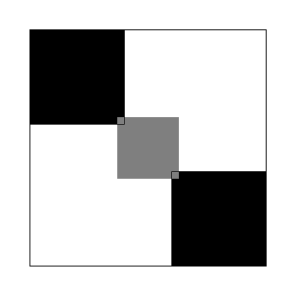
Figure 1. The graphon $W_{n}$.

Note that each $W_{n}$ is connected. Let $W$ be the graphon corresponding to the complete graph on $2$ vertices. It is clear that $W_{n}$ converges to $W$ in the $L^{1}$-norm. Let us estimate the Cheeger constant of $W_{n}$. Define $A_{n}$ as the interval $(1/2-e^{-n}-1/n,1/2+e^{-n}+1/n)$. Then

(5.3) $$h_{W_{n}}\leq h_{W_{n}}(A_{n})=\frac{2\times e^{-n}\times\frac{2}{n}}{\frac{2}{n}\times\left(\frac{2}{n}+2e^{-n}\right)}$$

Thus $h_{W_{n}}\to 0$ as $n\to\infty$. But $h_{W}=1/2$ and thus we see that the Cheeger constant of $W_{n}$ does not converge to that of $W$.

5.2. Buser Inequality for Graphons

Theorem 5.1 (Buser Inequality).

Let $W$ be a connected graphon. Then

(5.4) $$\lambda_{W}\leq 2h_{W}\text{ and }\lambda_{W}\leq g_{W}$$

Proof.

We adapt the proof of Lemma 2.1 in [Chu97]. Let $A\sqcup B$ form a measurable partition of $I$ with $0<\mu_{L}(A)<1$. Define $f:I\to\mathbf{R}$ as

(5.5) $$f(x)=\left\{\begin{array}[]{ll}\displaystyle\frac{1}{\operatorname{vol}(A)}&\mbox{if }x\in A\\ -\displaystyle\frac{1}{\operatorname{vol}(B)}&\mbox{if }x\in B\end{array}\right.$$

Then $f\in{\textbf{1}}^{\perp}_{v}$. Now

(5.6) $$\begin{split}\lambda_{W}&\leq\frac{\|df\|^{2}_{e}}{\|f\|^{2}_{v}}\\ &=\frac{\int_{E}(f(x)-f(y))^{2}W(x,y)\ dydx}{\int_{0}^{1}f(x)^{2}d_{W}(x)\ dx}\\ &=\frac{\int_{I\times I}(f(x)-f(y))^{2}W(x,y)\ dydx}{2\int_{0}^{1}f(x)^{2}d_{W}(x)\ dx}\\ &=\frac{\int_{A\times B}(f(x)-f(y))^{2}W(x,y)\ dydx+\int_{B\times A}(f(x)-f(y))^{2}W(x,y)\ dydx}{2\left[\int_{A}f(x)^{2}d_{W}(x)\ dx+\int_{B}f(x)^{2}d_{W}(x)\ dx\right]}\\ &=\frac{\left(\frac{1}{\operatorname{vol}(A)}+\frac{1}{\operatorname{vol}(B)}\right)^{2}\left(\int_{A\times B}W(x,y)\ dxdy+\int_{B\times A}W(x,y)\ dxdy\right)}{2\left[\frac{1}{\operatorname{vol}(A)^{2}}\operatorname{vol}(A)+\frac{1}{\operatorname{vol}(B)^{2}}\operatorname{vol}(B)\right]}\\ &=\left(\frac{1}{\operatorname{vol}(A)}+\frac{1}{\operatorname{vol}(B)}\right)\int_{A\times B}W(x,y)\ dxdy\\ &\leq 2\frac{\int_{A\times B}W}{\min\{\operatorname{vol}(A),\operatorname{vol}(B)\}}\end{split}$$

Since $B=A^{c}$, and since the above holds for all choices of $A$ with $0<\mu_{L}(A)<1$, we have $\lambda_{W}\leq 2h_{W}$. From the penultimate inequality above we also get

(5.7) $$\lambda_{W}\leq\displaystyle\frac{\int_{A\times B}W(x,y)\ dxdy}{\operatorname{vol}(A)\operatorname{vol}(B)}$$

since $\operatorname{vol}(A)+\operatorname{vol}(B)\leq 1$. This leads to $\lambda_{W}\leq g_{W}$. ∎

5.3. The Co-area Formula for Graphons

Consider a finite graph $G=(V,E)$ and let $f:V\to\mathbf{R}$ be any map. Orient the edges of $G$ in such a way that for each oriented edge $e$ we have $f(e^{+})\geq f(e^{-})$. Let $\gamma_{0}<\gamma_{1}<\cdots<\gamma_{k}$ be all the reals in the image of $f$. Define $S_{i}=\{v\in V:\ f(v)\geq\gamma_{i}\}$. Then we have

(5.8) $$\sum_{e\in E}df(e)=\sum_{i=1}^{m}(\gamma_{i}-\gamma_{i-1})|E(S_{i}^{c},S_{i})|$$

where $E(S_{i}^{c},S_{i})$ denotes the set of all the edges in $G$ which have their tails in $S_{i}^{c}$ and heads in $S_{i}$. To see why Equation 5.8 is true, we fix an edge $e$ and see how much it contributes to the sum on the RHS. We add $\gamma_{i}-\gamma_{i-1}$ for each $i$ such that $e^{-}\in S_{i}^{c}$ and $e^{+}\in S_{i}$. This adds up to a total of $df(e)$, which is the same as the contribution of $e$ to the LHS.

If $G$ were a weighted graph with weight function $w:E\to\mathbf{R}^{+}$, Equation 5.8 takes the form

(5.9) $$\sum_{e\in E}df(e)w(e)=\sum_{i=1}^{m}(\gamma_{i}-\gamma_{i-1})e_{w}(S_{i}^{c},S_{i})$$

where $e_{w}(S_{i}^{c},S_{i})$ denotes the sum of weights of all the edges which have their tails in $S_{i}^{c}$ and heads in $S_{i}$.

Let us see how Equation 5.9 generalizes for graphons. Let $W$ be a graphon and $f:I\to\mathbf{R}$ be in $L^{2}(I,\nu)$. Define $E_{f}$ to be the set $\{(x,y)\in I^{2}:\ f(y)>f(x)\}$. Let $S_{t}$ denote the set $f^{-1}(t,\infty)$. Then

(5.10) $$\int_{E_{f}}df(x,y)W(x,y)\ dxdy=\int_{-\infty}^{\infty}e_{W}(S_{t}^{c},S_{t})\ dt$$

This can be easily proved using Fubini’s theorem. We shall however need a slight variant of this formula in order to establish Cheeger’s inequality.

Theorem 5.2 (Co-area formula for graphons).

Let $W$ be a graphon and $f:I\to\mathbf{R}$ be an arbitrary map in $L^{2}(I,\nu)$. Define $f_{+}:I\to\mathbf{R}$ and $f_{-}:I\to\mathbf{R}$ as $f_{+}=\max\{f,0\}$ and $f_{-}=-\min\{f,0\}$. Let $S_{t}=f^{-1}(t,\infty)$. Then

(5.11) $$\begin{split}\int_{E_{f}}|df^{2}_{+}|W&=\int_{0}^{\infty}e_{W}(S_{\sqrt{t}}^{c},S_{\sqrt{t}})\ dt=\int_{0}^{\infty}2te_{W}(S_{t}^{c},S_{t})\ dt,\quad\text{and}\\ \int_{E_{f}}|df_{-}^{2}|W&=\int_{0}^{\infty}e_{W}(S_{-\sqrt{t}}^{c},S_{-\sqrt{t}})=\int_{0}^{\infty}2te_{W}(S_{-t}^{c},S_{-t})\ dt\end{split}$$

Proof.

We prove the first one. The second one is similar. We have by change of variables that

(5.12) $$\int_{0}^{\infty}e_{W}(S_{\sqrt{t}}^{c},S_{\sqrt{t}})\ dt=\int_{0}^{\infty}2te_{W}(S_{t}^{c},S_{t})\ dt$$

Now

(5.13) $$\begin{split}\int_{0}^{\infty}2te_{W}(S_{t}^{c},S_{t})\ dt&=\int_{0}^{\infty}2t\left[\int_{S_{t}^{c}\times S_{t}}W(x,y)\ dxdy\right]dt\\ &=\int_{0}^{\infty}\left[\int_{I^{2}}2t\chi_{S_{t}^{c}\times S_{t}}(x,y)W(x,y)\ dxdy\right]dt\\ &=\int_{I^{2}}\left[\int_{0}^{\infty}2t\chi_{S_{t}^{c}\times S_{t}}(x,y)W(x,y)\ dt\right]dxdy\\ &=\int_{I^{2}}\left[\int_{0}^{\infty}2t\chi_{S_{t}^{c}\times S_{t}}(x,y)\ dt\right]W(x,y)dxdy\\ &=\int_{E_{f}}\left[\int_{0}^{\infty}2t\chi_{S_{t}^{c}\times S_{t}}(x,y)\ dt\right]W(x,y)dxdy\\ &=\int_{E_{f}}\left[\int_{f_{+}(x)}^{f_{+}(y)}2t\ dt\right]W(x,y)dxdy\\ &=\int_{E_{f}}(f_{+}^{2}(y)-f_{+}^{2}(x))W(x,y)\ dxdy\\ &=\int_{E_{f}}|df^{2}_{+}|W\end{split}$$

as desired. ∎

5.4. Cheeger’s Inequality for Graphons

In this subsection we will prove the following.

Theorem 5.3.

Let $W$ be a connected graphon. Then

(5.14) $$\lambda_{W}\geq\frac{h^{2}_{W}}{8}$$

Before we prove Cheeger’s inequality above, we first obtain a more convenient formula (Lemma 5.4 below) for $\lambda_{W}$. Consider the map $\mathcal{I}:L^{2}(I,\nu)\to\mathbf{R}$ defined as

(5.15) $$\mathcal{I}(f)=\int_{0}^{1}f(x)d_{W}(x)\ dx=\langle f,{\textbf{1}}\rangle_{v}$$

We show that $L^{\infty}(I)\cap{\textbf{1}}^{\perp}_{v}$ is dense in ${\textbf{1}}^{\perp}_{v}$. Let $P:L^{2}(I,\nu)\to L^{2}(I,\nu)$ be the map defined as $P(f)=f-\mathcal{I}(f)$. Then $P$ is a bounded linear operator. Also, we have

(5.16) $$P^{2}(f)=P(f-\mathcal{I}(f))=f-\mathcal{I}(f)=P(f)$$

So $P^{2}=P$. Further,

(5.17) $$\begin{split}\langle Pf,g\rangle_{v}-\langle f,Pg\rangle_{v}&=\langle f-\mathcal{I}(f),g\rangle_{v}-\langle f,g-\mathcal{I}(g)\rangle_{v}\\ &=-\langle\mathcal{I}(f),g\rangle_{v}+\langle f,\mathcal{I}(g)\rangle_{v}\\ &=-\mathcal{I}(f)\mathcal{I}(g)+\mathcal{I}(f)\mathcal{I}(g)\\ &=0\end{split}$$

Therefore $P$ is self-adjoint. This means that $P$ is the orthogonal projection onto its image. It is clear that $\operatorname{Im}(P)\subseteq{\textbf{1}}^{\perp}_{v}$, and also that $P$ behaves as the identity when restricted to ${\textbf{1}}^{\perp}_{v}$. Therefore $P$ is the orthogonal projection onto ${\textbf{1}}^{\perp}_{v}$. It is also clear that $P(L^{\infty}(I))\subseteq L^{\infty}(I)$. We conclude that $L^{\infty}(I)\cap{\textbf{1}}^{\perp}_{v}$ is dense in ${\textbf{1}}^{\perp}_{v}$.

Now let $g\in{\textbf{1}}^{\perp}_{v}$ be an arbitrary nonzero vector. Then both $\|dg\|_{e}$ and $\|g\|_{v}$ are nonzero. Let $M>0$ be such that $\|dg\|_{e},\|g\|_{v}\geq M$. Let $\varepsilon>0$ be arbitrary and choose $g^{\prime}\in L^{\infty}(I)\cap{\textbf{1}}^{\perp}_{v}$ such that $\|g-g^{\prime}\|_{v}<\varepsilon M$. We had shown in the proof of Lemma 3.3, $\|df\|_{e}\leq 2\|f\|_{v}$ for all $f\in L^{2}(I,\nu)$. So

$$\|d(g-g^{\prime})\|_{e}=\|dg-dg^{\prime}\|_{e}<2\varepsilon M.$$

Thus we have

$$|\|g\|_{v}-\|g^{\prime}\|_{v}|<\varepsilon M\text{ and }|\|dg\|_{e}-\|dg^{\prime}\|_{e}|<2\varepsilon M$$

Hence we can approximate $\|dg\|_{e}/\|g\|_{v}$ arbitrarily well by the expressions of the form $\|dg^{\prime}\|_{e}/\|g^{\prime}\|_{v}$ by choosing a suitable $g^{\prime}\in L^{\infty}(I)\cap{\textbf{1}}^{\perp}_{v}$. We have proved

Lemma 5.4.

Let $W$ be a connected graphon. Then

(5.18) $$\lambda_{W}=\inf_{g\in{\textbf{1}}^{\perp}_{v}:\ g\neq 0}\frac{\|dg\|_{e}^{2}}{\|g\|_{v}^{2}}=\inf_{\begin{subarray}{c}g\in{\textbf{1}}^{\perp}_{v}:\ g\neq 0,\\ g\in L^{\infty}(I)\end{subarray}}\frac{\|dg\|_{e}^{2}}{\|g\|_{v}^{2}}$$

Now we are ready to prove Theorem 5.3. Let $g:I\to\mathbf{R}$ be an arbitrary map in $L^{\infty}(I)$ with $\|g\|_{v}=1$ and $\langle g,{\textbf{1}}\rangle_{v}=0$. To prove Theorem 5.3 it suffices to show that $\|dg\|_{e}^{2}\geq\frac{1}{8}h^{2}_{W}$. Let

(5.19) $$t_{0}=\sup\{t\in\mathbf{R}:\ \operatorname{vol}_{W}(g^{-1}(-\infty,t))\leq\frac{1}{2}\operatorname{vol}_{W}(I)\}$$

The number $t_{0}$ exists since $g$ is $L^{\infty}$. Define $f=g-t_{0}$. Then both the sets $\{f<0\}$ and $\{f>0\}$ have volumes at most half of $\operatorname{vol}_{W}(I)$. Also

(5.20) $$\|f\|_{v}^{2}=\|g-t_{0}\|_{v}^{2}=\|g\|_{v}^{2}+\|t_{0}\|_{v}^{2}-2t_{0}\langle g,{\textbf{1}}\rangle_{v}=1+\|t_{0}\|_{v}^{2}\geq 1$$

Clearly, $df=dg$. Therefore

(5.21) $$\|dg\|_{e}^{2}\geq\frac{\|df\|_{e}^{2}}{\|f\|_{v}^{2}}$$

Lemma 5.5.

(5.22) $$\|df\|_{e}^{2}\geq\frac{1}{8\|f\|_{v}^{2}}\left[\int_{E_{f}}|df^{2}_{+}|W+\int_{E_{f}}|df^{2}_{-}|W\right]^{2}$$

Proof.

Note that

(5.23) $$\|df\|_{e}^{2}=\int_{E}|df|^{2}W=\int_{E_{f}}|df|^{2}W$$

where $E_{f}=\{(x,y)\in I^{2}:\ f(y)>f(x)\}$. Also

(5.24) $$\int_{E_{f}}|df|^{2}W\geq\int_{E_{f}}|df_{+}|^{2}W+\int_{E_{f}}|df_{-}|^{2}W$$

This is because $|df|^{2}\geq|df_{+}|^{2}+|df_{-}|^{2}$ is true pointwise in $E_{f}$. By Cauchy-Schwarz we have

(5.25) $$\begin{split}\left[\int_{E_{f}}|df_{+}|^{2}W\right]^{1/2}\left[\int_{I^{2}}(|f(x)|+|f(y)|)^{2}W(x,y)\ dxdy\right]^{1/2}&\geq\int_{E_{f}}|df^{2}_{+}|W\\ \end{split}$$

Using Cauchy-Schwarz again, we can show that

(5.26) $$4\|f\|_{v}^{2}\geq\int_{I^{2}}(|f(x)|+|f(y)|)^{2}W(x,y)\ dxdy$$

which gives

(5.27) $$\begin{split}2\|f\|_{v}\left[\int_{E_{f}}|df_{+}|^{2}W\right]^{1/2}&\geq\int_{E_{f}}|df_{+}^{2}|W\\ \Rightarrow\int_{E_{f}}|df_{+}|^{2}W&\geq\frac{1}{4\|f\|_{v}^{2}}\left(\int_{E_{f}}|df_{+}^{2}|W\right)^{2}\end{split}$$

Similarly,

(5.28) $$\int_{E_{f}}|df_{-}|^{2}W\geq\frac{1}{4\|f\|_{v}^{2}}\left(\int_{E_{f}}|df_{-}^{2}|W\right)^{2}$$

Using these in Equation 5.24 gives

(5.29) $$\begin{split}\int_{E_{f}}|df|^{2}W&\geq\frac{1}{4\|f\|_{v}^{2}}\left[\left(\int_{E_{f}}|df_{+}^{2}|W\right)^{2}+\left(\int_{E_{f}}|df_{-}^{2}|W\right)^{2}\right]\\ &\geq\frac{1}{8\|f\|_{v}^{2}}\left[\int_{E_{f}}|df^{2}_{+}|W+\int_{E_{f}}|df^{2}_{-}|W\right]^{2}\end{split}$$

and we have proved the lemma. ∎

We now proceed to complete the proof of Theorem 5.3.

Proof of Theorem 5.3:
The Co-area Formula Theorem 5.2 gives

(5.30) $$\int_{E_{f}}|df^{2}_{+}|W=\int_{0}^{\infty}2te_{W}(S_{t}^{c},S_{t})\ dt\quad\text{ and }\quad\int_{E_{f}}|df_{-}^{2}|W=\int_{0}^{\infty}2te_{W}(S_{-t}^{c},S_{-t})\ dt$$

But

(5.31) $$\begin{split}\int_{0}^{\infty}2te_{W}(S_{t}^{c},S_{t})\ dt&\geq h_{W}\int_{0}^{\infty}2t\operatorname{vol}(S_{t})\ dt\\ &=h_{W}\int_{0}^{\infty}2t\left[\int_{I^{2}}\chi_{I\times S_{t}}(x,y)W(x,y)\ dxdy\right]dt\\ &=h_{W}\int_{I^{2}}\left[\int_{0}^{\infty}2t\chi_{I\times S_{t}}(x,y)\ dt\right]W(x,y)dxdy\\ &=h_{W}\int_{I^{2}}\left[\int_{0}^{\infty}2t\chi_{I\times S_{t}}(x,y)\ dt\right]W(x,y)dxdy\\ &=h_{W}\int_{I^{2}}\left[\int_{0}^{f_{+}(y)}2t\ dt\right]W(x,y)\ dxdy\\ &=h_{W}\int_{I^{2}}f_{+}^{2}(y)W(x,y)\ dxdy\end{split}$$

Similarly

(5.32) $$\begin{split}\int_{0}^{\infty}2te_{W}(S_{-t}^{c},S_{-t})\ dt&\geq h_{W}\int_{0}^{\infty}2t\operatorname{vol}(S_{-t}^{c})\ dt\\ &=h_{W}\int_{0}^{\infty}2t\left[\int_{I^{2}}\chi_{I\times S_{-t}^{c}}(x,y)W(x,y)\ dxdy\right]dt\\ &=h_{W}\int_{I^{2}}\left[\int_{0}^{\infty}2t\chi_{I\times S_{-t}^{c}}(x,y)\ dt\right]W(x,y)dxdy\\ &=h_{W}\int_{I^{2}}\left[\int_{0}^{\infty}2t\chi_{I\times S_{-t}^{c}}(x,y)\ dt\right]W(x,y)dxdy\\ &=h_{W}\int_{I^{2}}\left[\int_{0}^{f_{-}(y)}2t\ dt\right]W(x,y)dxdy\\ &=h_{W}\int_{I^{2}}f_{-}^{2}(y)W(x,y)\ dxdy\end{split}$$

Therefore

(5.33) $$\begin{split}\int_{E_{f}}|df^{2}_{+}|W+\int_{E_{f}}|df^{2}_{-}|W&\geq h_{W}\left[\int_{I^{2}}f_{+}^{2}(y)W(x,y)\ dxdy+\int_{I^{2}}f_{-}^{2}(y)W(x,y)\ dxdy\right]\\ &=h_{W}\left[\int_{I^{2}}(f_{+}^{2}(y)+f_{-}^{2}(y))W(x,y)\ dxdy\right]\\ &=h_{W}\left[\int_{I^{2}}f^{2}(y)W(x,y)\ dxdy\right]\\ &=h_{W}\left[\int_{I}f^{2}(y)d_{W}(y)\ dy\right]=h_{W}\|f\|^{2}_{v}\end{split}$$

Combining this with Lemma 5.5, we have

(5.34) $$\|df\|_{e}^{2}\geq\frac{1}{8\|f\|_{v}^{2}}h^{2}_{W}\|f\|_{v}^{4}$$

and thus

(5.35) $$\frac{\|df\|_{e}^{2}}{\|f\|_{v}^{2}}\geq\frac{1}{8}h^{2}_{W}$$

Lastly, using Equation 5.21 we have

(5.36) $$\|dg\|_{e}^{2}\geq\frac{1}{8}h^{2}_{W}$$

and we are done. $\blacksquare$

6. Cheeger Constant for Graphings and the Cheeger-Buser Inequalities

We now turn to graphings. For the purposes of this section $G=(I,\mu,E)$ will denote a graphing. As discussed in Section 2.2, graphings are substantially different from graphons in terms of their structure. In spite of this difference, Lemma 2.4 will allow us to furnish proofs that are, at least at a formal level, extremely similar to the proofs in Section 3 above. However, the actual intuition and idea behind the proofs will really go back to Theorem 2.3. In this section, we shall therefore try to convey to the reader both the formal similarity with the proofs in Section 3 as well as the actual structural idea going back to Theorem 2.3.

6.1. Cheeger Constant for Graphings

For two measurable subsets $A$ and $B$ of $I$, we define

(6.1) $$e_{G}(A,B)=\eta(A,B)=\int_{A}\deg_{B}(x)\ d\mu(x)$$

For a measurable subset $A$ of $I$, the volume of $G$ over $A$ is defined as

(6.2) $$\operatorname{vol}(A)=\int_{A}\deg(x)\ d\mu(x)=e_{G}(A,I)$$

A graphing is said to be connected if for all measurable subsets $A$ of $I$ with $0<\mu(A)<1$ we have $e_{G}(A,A^{c})\neq 0$. Note that if $G$ is connected then $\deg>0$ a.e.

Given a graphing $G$, we define the Cheeger constant of $G$ as

(6.3) $$h_{G}=\inf_{A\subseteq I:\ 0<\mu(A)<1}\frac{e_{G}(A,A^{c})}{\min\{\operatorname{vol}(A),\operatorname{vol}(A^{c})\}}$$

A symmetrized version of the above constant which we will be referred to as the symmetric Cheeger constant is defined as

(6.4) $$g_{G}=\inf_{A\subseteq I:\ 0<\mu(A)<1}\frac{e_{G}(A,B)}{\operatorname{vol}(A)\operatorname{vol}(A^{c})}$$

Note that the above defined constants exist for connected graphings.

6.2. Buser Inequality for Graphings

We first observe that the multiplicity of the singular value $0$ of the Laplacian of a connected graphing $(I,\mu,E)$ is 1. For $f\in L^{2}(I,\mu)$, we have $\Delta f=0$ if and only if $df=0$. As in the case of graphons it now suffices to show the following: $df=0$ if and only if $f$ is constant (up to a set of measure zero). Of course, $df=0$ for constant $f$. Conversely, assume that $df=0$. Then

(6.5) $$\int_{E^{+}}(df)^{2}\ d\eta=0$$

which implies that

(6.6) $$\int_{E^{+}}(f(y)-f(x))^{2}\ d\eta(x,y)=0.$$

Since

(6.7) $$\int_{E^{+}}(f(y)-f(x))^{2}\ d\eta(x,y)=\int_{E^{-}}(f(y)-f(x))^{2}\ d\eta(x,y).$$

it follows that

(6.8) $$\int_{I^{2}}(f(y)-f(x))^{2}\ d\eta(x,y)=0$$

For each $t\in\mathbf{R}$, let $S_{t}=f^{-1}(t,\infty)$. Therefore,

(6.9) $$\int_{S_{t}^{c}\times S_{t}}(f(y)-f(x))^{2}\ d\eta(x,y)=0.$$

It follows that $(f(y)-f(x))^{2}$ is $\eta$-a.e. $0$ on $S_{t}^{c}\times S_{t}$. But $f(y)-f(x)\neq 0$ for all $(x,y)\in S_{t}\times S_{t}^{c}$. So $\eta(S_{t}^{c},S_{t})=0$ for all $t$. The connectedness of $G$ then implies that either $S_{t}$ or $S_{t}^{c}$ has $\mu$-measure $0$. So our claim follows from the following lemma whose proof is an exact replica of Lemma 3.5 and we omit it.

Lemma 6.1.

Let $f:I\to\mathbf{R}$ be a measurable function such that for all $t\in\mathbf{R}$ we have either $f^{-1}(-\infty,t]$ or $f^{-1}(t,\infty)$ has $\mu$-measure $0$. Then $f$ is constant $\mu$-a.e.

The eigenfunctions corresponding to $0$ are thus the essentially constant functions: the $0-$eigenspace of $\Delta$ is generated by 1. Define

(6.10) $$\lambda_{G}=\inf_{g\in{\textbf{1}}^{\perp}_{v}:\ g\neq 0}\frac{\langle g,\Delta g\rangle_{v}}{\langle g,g\rangle_{v}}=\inf_{g\in{\textbf{1}}^{\perp}_{v}:\ g\neq 0}\frac{\|dg\|^{2}_{e}}{\|g\|^{2}_{v}}$$

(Here, ${\textbf{1}}^{\perp}_{v}$ denotes the orthogonal complement of 1 with respect to the inner product $\langle\cdot,\cdot\rangle_{v}$).

Theorem 6.2 (Buser Inequality).

Let $G=(I,\mu,E)$ be a connected graphing. Then

(6.11) $$\lambda_{G}\leq 2h_{G}\text{ and }\lambda_{G}\leq g_{G}$$

The proof below exploits the fact that one can decompose a graphing into finitely many matchings (Theorem 2.3). An alternate proof can also be given following that of Theorem 5.4 replacing $W(x,y)dxdy$ formally with $d\eta(x,y)$.

Proof.

Let $\varphi_{i}:C_{i}\to C_{i}$, $1\leq i\leq k$, be $\mu$-measure preserving involutions such that

(6.12) $$E=\bigsqcup_{i=1}^{k}\{(x,\varphi_{i}(x)):\ x\in C_{i}\}$$

Extend each $\varphi_{i}$ to a map $\varphi_{i}:I\to I$ by declaring $\varphi_{i}(x)=x$ for all $x\notin C_{i}$. Let $A\sqcup B$ form a measurable partition of $I$ with $0<\mu(A)<1$. Define $f:I\to\mathbf{R}$ as

(6.13) $$f(x)=\left\{\begin{array}[]{ll}\displaystyle\frac{1}{\operatorname{vol}(A)}&\mbox{if }x\in A\\ -\displaystyle\frac{1}{\operatorname{vol}(B)}&\mbox{if }x\in B\end{array}\right.$$

Then $f\in{\textbf{1}}^{\perp}_{v}$. Now

$$\begin{split}\lambda_{G}&\leq\frac{\|df\|^{2}_{e}}{\|f\|^{2}_{v}}=\frac{\int_{E^{+}}(f(x)-f(y))^{2}\ d\eta(x,y)}{\int_{0}^{1}f(x)^{2}\deg(x)\ d\mu(x)}=\frac{\int_{I^{2}}(f(x)-f(y))^{2}\ d\eta(x,y)}{2\int_{0}^{1}f(x)^{2}\deg(x)\ d\mu(x)}\\ &=\frac{\sum_{i=1}^{k}\int_{I}(f(x)-f(\varphi_{i}(x)))^{2}\ d\mu(x)}{2\int_{0}^{1}f(x)^{2}\deg(x)\ d\mu(x)}\\ &=\frac{\sum_{i=1}^{k}\left[\int_{A}(f(x)-f(\varphi_{i}(x)))^{2}\ d\mu(x)+\int_{B}(f(x)-f(\varphi_{i}(x)))^{2}\ d\mu(x)\right]}{2\int_{0}^{1}f(x)^{2}\deg(x)\ d\mu(x)}\\ &=\frac{\sum_{i=1}^{k}\left[\int_{A}(f(x)-f(\varphi_{i}(x)))^{2}\chi_{B}(\varphi_{i}(x))\ d\mu(x)-\int_{B}(f(x)-f(\varphi_{i}(x)))^{2}\chi_{A}(\varphi_{i}(x))\ d\mu(x)\right]}{2\int_{0}^{1}f(x)^{2}\deg(x)\ d\mu(x)}\\ &=\frac{\sum_{i=1}^{k}\left[\int_{A}\left(\frac{1}{\operatorname{vol}(A)}+\frac{1}{\operatorname{vol}(B)}\right)^{2}\chi_{B}(\varphi_{i}(x))\ d\mu(x)+\int_{B}\left(\frac{1}{\operatorname{vol}(B)}+\frac{1}{\operatorname{vol}(A)}\right)^{2}\chi_{A}(\varphi_{i}(B))\ d\mu(x)\right]}{2\int_{0}^{1}f(x)^{2}\deg(x)\ d\mu(x)}\\ &=\frac{\left(\frac{1}{\operatorname{vol}(A)}+\frac{1}{\operatorname{vol}(B)}\right)^{2}\sum_{i=1}^{k}\left[\int_{A}\chi_{B}(\varphi_{i}(x))\ d\mu(x)+\int_{B}\chi_{A}(\varphi_{i}(x))\ d\mu(x)\right]}{2\left[\int_{A}f(x)^{2}\deg(x)\ d\mu(x)+\int_{B}f(x)^{2}\deg(x)\ d\mu(x)\right]}\\ &=\frac{\left(\frac{1}{\operatorname{vol}(A)}+\frac{1}{\operatorname{vol}(B)}\right)^{2}\left[\int_{A}\deg_{B}(x)\ d\mu(x)+\int_{B}\deg_{A}(x)\ d\mu(x)\right]}{2\left[\frac{1}{\operatorname{vol}(A)^{2}}\operatorname{vol}(A)+\frac{1}{\operatorname{vol}(B)^{2}}\operatorname{vol}(B)\right]}\\ &=\left(\frac{1}{\operatorname{vol}(A)}+\frac{1}{\operatorname{vol}(B)}\right)e_{G}(A,B)\\ &\leq 2\frac{e_{G}(A,B)}{\min\{\operatorname{vol}(A),\operatorname{vol}(B)\}},\frac{e_{G}(A,B)}{\operatorname{vol}(A)\operatorname{vol}(B)}\end{split}$$

Since $B=A^{c}$, and since the above holds for all choices of $A$ with $0<\mu(A)<1$, we have $\lambda_{G}\leq 2h_{G}$ and $\lambda_{G}\leq g_{G}$. ∎

Alternate Proof: In the proof of Theorem 5.4 replace $W(x,y)dxdy$ formally with $d\eta(x,y)$. $\blacksquare$

6.3. Co-area Formula for Graphings

Let $G=(I,E,\mu)$ be a graphing and $f:I\to\mathbf{R}$ be any $L^{\infty}$-map. Let $E_{f}$ be defined as

(6.14) $$E_{f}=\{(x,y)\in E:\ f(y)>f(x)\}$$

The set $E_{f}$ will be referred to as the $f$-oriented edges of $G$. Let $S_{t}$ denote the set $f^{-1}(t,\infty)$. Then

(6.15) $$\int_{E_{f}}dfd\eta=\int_{-\infty}^{\infty}e_{G}(S_{t}^{c},S_{t})\ dt$$

Let us see the proof in the special case when $E$ is given by a single measure preserving involution $\varphi:A\to A$ where $A$ is a measurable subset of $I$. Define $R=\{x\in A:\ (x,\varphi(x))\in E_{f}\}$. Then the RHS of the above equation is

(6.16) $$\begin{split}\int_{-\infty}^{\infty}e_{G}(S_{t}^{c},S_{t})\ dt&=\int_{-\infty}^{\infty}\int_{S_{t}^{c}}\deg_{S_{t}}(x)\ d\mu(x)\ dt=\int_{-\infty}^{\infty}\int_{0}^{1}\chi_{S_{t}^{c}}(x)\deg_{S_{t}}(x)\ d\mu(x)\ dt\\ &=\int_{0}^{1}\int_{-\infty}^{\infty}\chi_{S_{t}^{c}}(x)\deg_{S_{t}}(x)\ dt\ d\mu(x)=\int_{0}^{1}\int_{f(x)}^{\infty}\deg_{S_{t}}(x)\ dt\ d\mu(x)\\ &=\int_{R}\int_{f(x)}^{\infty}\deg_{S_{t}}(x)\ dt\ d\mu(x)=\int_{R}(f\circ\varphi(x)-f(x))\ d\mu(x)\end{split}$$

On the other hand the LHS of Equation 6.15 is

(6.17) $$\begin{split}\int_{E_{f}}df\ d\eta=\int_{I^{2}}df\chi_{E_{f}}\ d\eta&=\int_{I}\sum_{y}df(x,y)\chi_{E_{f}}(x,y)\ d\mu(x)\\ &=\int_{R}df(x,\varphi(x))\ d\mu(x)\\ &=\int_{R}(f\circ\varphi(x)-f(x))\ d\mu(x)\end{split}$$

and therefore Equation 6.15 holds. Just as in the case of graphons, we need a slightly different lemma

Theorem 6.3.

Let $G=(I,E,\mu)$ be a graphing and $f:I\to\mathbf{R}$ be an arbitrary $L^{2}$-map. Define $f_{+}:I\to\mathbf{R}$ and $f_{-}:I\to\mathbf{R}$ as the map $f_{+}=\max\{f,0\}$ and $f_{-}=-\min\{f,0\}$. Let $S_{t}=f^{-1}(t,\infty)$. Then

(6.18) $$\begin{split}\int_{E_{f}}|df^{2}_{+}|\ d\eta&=\int_{0}^{\infty}e_{G}(S_{\sqrt{t}}^{c},S_{\sqrt{t}})\ dt=\int_{0}^{\infty}2te_{G}(S_{t}^{c},S_{t})\ dt,\quad\text{and}\\ \int_{E_{f}}|df_{-}^{2}|\ d\eta&=\int_{0}^{\infty}e_{G}(S_{-\sqrt{t}}^{c},S_{-\sqrt{t}})=\int_{0}^{\infty}2te_{G}(S_{-t}^{c},S_{-t})\ dt\end{split}$$

Proof.

We prove only the first one. Further, as in the proof of Lemma 2.4 (see also Equation 2.17) we first assume that the edge set $E$ is determined by a single $\mu$-measure preserving involutions $\varphi:A\to A$ defined on a measurable subset $A$ of $I$. Define $E_{f}=\{(x,y)\in E:\ f(y)>f(x)\}$. Let $R=\{x\in I:\ (x,\varphi(x))\in E_{f}\}$. We have by change of variables that

(6.19) $$\int_{0}^{\infty}e_{G}(S_{\sqrt{t}}^{c},S_{\sqrt{t}})\ dt=\int_{0}^{\infty}2te_{G}(S_{t}^{c},S_{t})\ dt$$

Now

(6.20) $$\begin{split}\int_{0}^{\infty}2te_{G}(S_{t}^{c},S_{t})\ dt&=\int_{0}^{\infty}2t\eta(S_{t}^{c}\times S_{t})\ dt=\int_{0}^{\infty}2t\left[\int_{0}^{1}\chi_{S_{t}^{c}}(x)\deg_{S_{t}}(x)\ d\mu(x)\right]dt\\ &=\int_{0}^{\infty}\left[\int_{0}^{1}2t\chi_{S_{t}^{c}}(x)\deg_{S_{t}}(x)\ d\mu(x)\right]dt\\ &=\int_{0}^{1}\left[\int_{0}^{\infty}2t\chi_{S_{t}^{c}}(x)\deg_{S_{t}}(x)\ dt\right]d\mu(x)\\ &=\int_{0}^{1}\left[\int_{f_{+}(x)}^{\infty}2t\deg_{S_{t}}(x)\ dt\right]d\mu(x)\\ &=\int_{R}\left[\int_{f_{+}(x)}^{\infty}2t\deg_{S_{t}}(x)\ dt\right]d\mu(x)\\ &=\int_{R}\left[\int_{f_{+}(x)}^{f_{+}(\varphi(x))}2t\ dt\right]d\mu(x)\\ &=\int_{R}(f_{+}^{2}(\varphi(x))-f_{+}^{2}(x))d\mu(x)\end{split}$$

On the other hand

(6.21) $$\begin{split}\int_{E_{f}}|df_{+}^{2}|\ d\eta&=\int_{I^{2}}|df_{+}^{2}(x,y)|\chi_{E_{f}}(x,y)\ d\eta(x,y)\\ &=\int_{I}\sum_{y}|df_{+}^{2}(x,y)|\chi_{E_{f}}(x,y)\ d\mu(x)\\ &=\int_{R}|df_{+}^{2}(x,\varphi(x))|\ d\mu(x)\\ &=\int_{R}(f_{+}^{2}(\varphi(x))-f_{+}^{2}(x))\ d\mu(x),\end{split}$$

completing the proof for the special case of a single strand.

We now deal with the general case where there may be multiple strands. Let $\varphi_{i}:A_{i}\to A_{i}$, $1\leq i\leq k$, be $\mu$-measure preserving involutions such that $E=\bigsqcup_{i=1}^{k}\{(x,\varphi_{i}(x)):\ x\in A_{i}\}$. Let $G_{i}$ be the graphing corresponding to $\varphi_{i}$. So $G=\bigsqcup_{i=1}^{k}G_{i}$. Then

(6.22) $$\begin{split}\int_{0}^{\infty}2te_{G}(S_{t}^{c},S_{t})\ dt&=\sum_{i=1}^{k}\int_{0}^{\infty}2te_{G_{i}}(S_{t}^{c},S_{t})\ dt\end{split}$$

and

(6.23) $$\begin{split}\int_{E_{f}}|df_{+}^{2}|\ d\eta&=\sum_{i=1}^{k}\int_{E_{f}^{i}}|df_{+}^{2}|\ d\eta_{i}\end{split}$$

where $E_{f}^{i}$ are the $f$-oriented edges of $G_{i}$ and $\eta_{i}$ is the edge measure of $G_{i}$. Thus the general case follows from the special case. ∎

6.4. Cheeger Inequality for Graphings

In this subsection we will prove the following Cheeger inequality for graphings.

Theorem 6.4.

Let $G$ be a connected graphing. Then

(6.24) $$\lambda_{G}\geq\frac{h^{2}_{G}}{8}$$

The proof of Lemma 5.4 goes through mutatis mutandis to give:

Lemma 6.5.

Let $G$ be a connected graphing. Then

(6.25) $$\lambda_{G}=\inf_{g\in{\textbf{1}}^{\perp}_{v}:\ g\neq 0}\frac{\|dg\|_{e}^{2}}{\|g\|_{v}^{2}}=\inf_{\begin{subarray}{c}g\in{\textbf{1}}^{\perp}_{v}:\ g\neq 0,\\ g\in L^{\infty}(I,\mu)\end{subarray}}\frac{\|dg\|_{e}^{2}}{\|g\|_{v}^{2}}$$

We proceed with the proof of Theorem 6.4 for graphings. Let $g:I\to\mathbf{R}$ be an arbitrary $L^{\infty}$-map with $\|g\|_{v}=1$ and $\langle g,{\textbf{1}}\rangle_{v}=0$. To prove Cheeger’s inequality it is enough to show that $\|dg\|_{e}^{2}\geq\frac{1}{8}h^{2}_{G}$. Let

(6.26) $$t_{0}=\sup\{t\in\mathbf{R}:\ \operatorname{vol}_{G}(g^{-1}(-\infty,t))\leq\frac{1}{2}\operatorname{vol}_{G}(I)\}$$

and define $f=g-t_{0}$. Then both the sets $\{f<0\}$ and $\{f>0\}$ have volumes at most half of $\operatorname{vol}_{G}(I)$. Also

(6.27) $$\|f\|_{v}^{2}=\|g-t_{0}\|_{v}^{2}=\|g\|_{v}^{2}+\|t_{0}\|_{v}^{2}-2t_{0}\langle g,{\textbf{1}}\rangle_{v}=1+\|t_{0}\|_{v}^{2}\geq 1$$

Clearly, $df=dg$. Therefore

(6.28) $$\|dg\|_{e}^{2}\geq\frac{\|df\|_{e}^{2}}{\|f\|_{v}^{2}}$$

Lemma 6.6.

(6.29) $$\int_{E_{f}}|df|^{2}\ d\eta\geq\frac{1}{8\|f\|_{v}^{2}}\left[\int_{E_{f}}|df^{2}_{+}|\ d\eta+\int_{E_{f}}|df^{2}_{-}|\ d\eta\right]^{2}$$

Proof.

As in Lemma 5.5, we start by observing that

(6.30) $$\int_{E^{+}}|df|^{2}\ d\eta=\int_{E_{f}}|df|^{2}\ d\eta$$

The proof of Lemma 6.6 is now an exact replica of that of Lemma 5.5: the only extra point to note being that

(6.31) $$\begin{split}\int_{I^{2}}f(x)^{2}\ d\eta(x,y)&=\int_{I}\sum_{y}f(x)^{2}\chi_{E}(x,y)\ d\mu(x)=\int_{I}f(x)^{2}\deg(x)\ d\mu(x)=\|f\|_{v}^{2}\end{split}$$

We omit the details. ∎

The rest of the proof of Theorem 6.4 is quite similar to that of Theorem 5.3. However, since this is one of the main theorems of this paper, we include the details for completeness. The Co-area Formula Theorem 6.3 gives:

(6.32) $$\int_{E_{f}}|df^{2}_{+}|\ d\eta=\int_{0}^{\infty}2te_{G}(S_{t}^{c},S_{t})\ dt,\quad\text{and}\quad\int_{E_{f}}|df_{-}^{2}|\ d\eta=\int_{0}^{\infty}2te_{G}(S_{-t}^{c},S_{-t})\ dt$$

But

(6.33) $$\small\begin{split}\int_{0}^{\infty}2te_{G}(S_{t},S_{t})\ dt&\geq h_{G}\int_{0}^{\infty}2t\operatorname{vol}(S_{t})\ dt=h_{G}\int_{0}^{\infty}2t\left[\int_{S_{t}}\deg(x)\ d\mu(x)\right]\ dt\\ &=h_{G}\int_{0}^{\infty}2t\left[\int_{I}\chi_{S_{t}}(x)\deg(x)\ d\mu(x)\right]\ dt=h_{G}\int_{0}^{\infty}\int_{I}2t\chi_{S_{t}}(x)\deg(x)\ d\mu(x)dt\\ &=h_{G}\int_{I}\int_{0}^{\infty}2t\chi_{S_{t}}(x)\deg(x)\ dtd\mu(x)=h_{G}\int_{I}\left[\int_{0}^{\infty}2t\chi_{S_{t}}(x)\ dt\right]\deg(x)\ d\mu(x)\\ &=h_{G}\int_{I}\left[\int_{0}^{f_{+}(x)}2t\ dt\right]\deg(x)d\mu(x)\\ &=h_{G}\int_{I}f_{+}^{2}(y)\deg(x)\ d\mu(x)\end{split}$$

Similarly

(6.34) $$\small\begin{split}\int_{0}^{\infty}2te_{G}(S_{-t}^{c},S_{-t})\ dt&\geq h_{G}\int_{0}^{\infty}2t\operatorname{vol}(S_{-t}^{c})\ dt=h_{G}\int_{0}^{\infty}2t\left[\int_{S^{c}_{-t}}\deg(x)\ d\mu(x)\right]dt\\ &=h_{G}\int_{0}^{\infty}2t\left[\int_{I}\chi_{S_{-t}^{c}}(x)\deg(x)\ d\mu(x)\right]dt=h_{G}\int_{0}^{\infty}\int_{I}2t\chi_{S^{c}_{-t}}(x)\deg(x)\ d\mu(x)dt\\ &=h_{G}\int_{I}\int_{0}^{\infty}2t\chi_{S^{c}_{-t}}(x)\deg(x)\ dtd\mu(x)=h_{G}\int_{I}\left[\int_{0}^{\infty}2t\chi_{S^{c}_{-t}}(x)\ dt\right]\deg(x)d\mu(x)\\ &=h_{G}\int_{I}\left[\int_{0}^{f_{-}(x)}2t\ dt\right]\deg(x)d\mu(x)\\ &=h_{G}\int_{I}f_{-}^{2}(x)\deg(x)\ d\mu(x,y)\end{split}$$

Therefore

(6.35) $$\begin{split}\int_{E_{f}}|df^{2}_{+}|\ d\eta+\int_{E_{f}}|df^{2}_{-}|\ d\eta&\geq h_{G}\left[\int_{I}f_{+}^{2}(x)\deg(x)\ d\mu(x)+\int_{I}f_{-}^{2}(x)\deg(x)\ d\mu(x)\right]\\ &=h_{G}{\int_{I}(f_{+}^{2}(x)+f_{-}^{2}(x))\deg(x)\ d\mu(x)}\\ &=h_{G}\int_{I}f(x)^{2}\deg(x)\ d\mu(x)\\ &=h_{G}\|f\|^{2}_{v}\end{split}$$

Combining this with Equation 6.29, we have

(6.36) $$\int_{E_{f}}|df|^{2}\ d\eta\geq\frac{1}{8\|f\|_{v}^{2}}h^{2}_{G}\|f\|_{v}^{4}$$

This along with Equation 6.30 gives

(6.37) $$\frac{\|df\|_{e}^{2}}{\|f\|_{v}^{2}}=\frac{\int_{E}|df|^{2}\ d\eta}{\|f\|_{v}^{2}}\geq\frac{1}{8}h^{2}_{G}$$

Lastly, using Equation 6.28 we have

(6.38) $$\|dg\|_{e}^{2}\geq\frac{1}{8}h^{2}_{G}$$

and Theorem 6.4 follows. $\Box$

7. Cheeger constant and connectedness

7.1. A connected graphon with zero Cheeger constant

Recall that a graphon is connected if for all measurable subsets $A$ of $I$ with $0<\mu_{L}(A)<1$ we have $e_{W}(A,A^{c})\neq 0$. More generally, given a graphon $W$ and a measurable subset $S$ of $I$, we say that the restriction $W|_{S}$ is connected if for all measurable subsets $A$ of $S$ with $0<\mu_{L}(A)<\mu_{L}(S)$, we have

(7.1) $$\int_{A\times(S\setminus A)}W>0$$

Lemma 7.1.

Let $W$ be a graphon and $S$ and $T$ be measurable subsets of $I$ such that $S\cup T=I$ and $S\cap T$ has positive measure. Further assume that $W|_{S}$ and $W|_{T}$ are connected. Then $W$ is connected.

Proof.

Assume that $W$ is disconnected and let $A$ be a measurable subset of $I$ such that $0<\mu_{L}(A)<1$ and $e_{W}(A,A^{c})=0$. Then in particular we have

(7.2) $$\int_{(A\cap S)\times(A^{c}\cap S)}W=0\text{ and }\int_{(A\cap T)\times(A^{c}\cap T)}W=0$$

The connectedness of $W|_{S}$ implies that either $A\cap S$ or $A^{c}\cap S$ has full measure in $S$. Without loss of generality assume that $A\cap S$ has full measure in $S$. Again, by the connectedness of $W|_{T}$ we have that $A\cap T$ or $A^{c}\cap T$ has full measure in $T$. In the former case we would have that $A$ has full measure in $I$ since $I=S\cup T$. In the latter case the measure of $S\cap T$ would be $0$. In any case we get a contradiction. ∎

Example 7.2.

Consider the graphon $W$ given by the following figure.

Figure 2. Example of a connected graphon.

The graphon takes the value $1$ at all the shaded points and $0$ at all other points. It follows by repeated use of Lemma 7.1 that $W$ is connected.

Let $W$ be a graphon taking values in $\{0,1\}$. We call such a graphon a neighborhood graphon if $W^{-1}(1)$ contains an open neighborhood of the diagonal of the open square $(0,1)\times(0,1)$. Note that the graphon in Example 7.2 contains instead an open neighborhood of the diagonal of the closed square $I^{2}$.

Lemma 7.3.

Every neighborhood graphon is connected.

Proof.

Let $W$ be a neighborhood graphon. For each $n>2$ let $S_{n}$ denote the interval $(1/n,1-1/n)$. Each $W|_{S_{n}}$ is connected. This is because a copy of the graphon shown in Figure 2 is embedded in the restriction of $W$ over $S_{n}\times S_{n}$.

We argue by contradiction. Suppose that $W$ is disconnected. The there is $A\subseteq I$ with $0<\mu_{L}(A)<1$ such that $e_{W}(A,A^{c})=0$. Therefore for each $n$ we have $\int_{(A\cap S_{n})\times(S_{n}\setminus A)}W=0$. By connectedness of $W|_{S_{n}}$, we must have that for any $n>2$, either $\mu_{L}(A\subseteq S_{n})=\mu_{L}(S_{n})$ or $\mu_{L}(A\cap S_{n})=0$. If the former happens for some $n$, then it must happen for all $n$, and consequently $A$ is of full measure in $I$. The other possibility is that $\mu_{L}(A\cap S_{n})=0$ for all $n$, but then $A$ has measure $0$. So in any case, we have a contradiction. ∎

Example 7.4.

A particular way of constructing a neighborhood graphon is the following. Let $f:I\to I$ be a continuous map such that $f(x)>x$ for all $0<x<1$. Define a graphon $W_{f}$ as

$$W_{f}(x,y)=\left\{\begin{array}[]{ll}1&\text{if }x\leq y\leq f(x)\\ 0&\text{if }f(x)<y\\ W(y,x)&\text{if }x>y\end{array}\right.$$

In other words, $W_{f}$ takes the value $1$ in the region trapped between the graph of $f$ and the reflection of the graph of $f$ about the $y=x$ line, and is $0$ everywhere else. For example, let $f(x)=\sqrt{x}$. Then the following diagram illustrates what $W_{f}$ looks like.

Figure 3. An example of a neighborhood graphon: $W_{f}$ corresponding to $f(x)=\sqrt{x}$.

The graphon shown in Figure 2 is also an example of a neighborhood graphon arising as $W_{f}$ for a suitably chosen continuous map $f:I\to I$.

Example 7.5.

Unlike in the case of finite graphs, the Cheeger constant of a connected graphon may be zero, as illustrated by Figure 4. The graphon takes the value $1$ at all the shaded points, either gray or black, and the value $0$ at all the unshaded points. Call this graphon $W$.

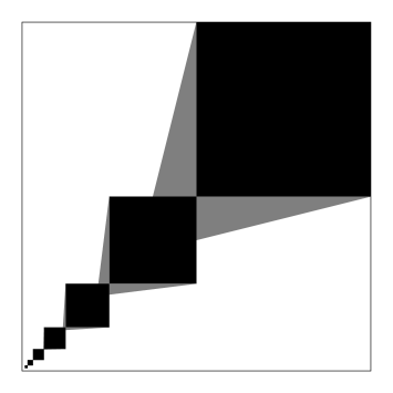
Figure 4. Example of a connected graphon whose Cheeger constant vanishes.

The bottom left endpoints of the black squares in the above figure have coordinates $(1/2^{n},1/2^{n})$, $n=1,2,3,\ldots$. The lengths of horizontal edges of the gray triangles above the $y=x$ line are $1/2^{2n+1}$, $n=1,2,3,\ldots$. Let $A_{n}$ be the interval $[0,1/2^{n}]$. Then $e(A_{n},A_{n}^{c})$ equals the measure of the gray region in $A^{n}\times A_{n}^{c}$. But there is only one gray triangle in this region. The sides of this right triangle (other than the hypotenuse) have lengths $1/2^{2n+1}$ and $1/2^{n}$. Thus $e(A_{n},A_{n}^{c})=1/2^{3n+2}$. Let $V$ denote the total measure of the points shaded black. Then $\operatorname{vol}(A_{n})\geq V/4^{n}+e(A_{n},A_{n}^{c})$ because the measure of the black region inside $A_{n}\times I$ is exactly $V/4^{n}$. For large $n$ we have $\operatorname{vol}(A_{n})$ is at most half the total volume. Thus for large $n$ we have

(7.3) $$h_{W}(A_{n})=\frac{e(A_{n},A_{n}^{c})}{\operatorname{vol}(A_{n})}\leq\frac{1/2^{3n+2}}{V/4^{n}+1/2^{3n+2}}=\frac{1/2^{n+2}}{V+1/2^{n+2}}$$

This is zero in the limit and thus the Cheeger constant of this graphon is zero. This graphon is connected by Lemma 7.3 because it is a neighborhood graphon.

7.2. A connected graphing with zero Cheeger constant

We prove in this section that the irrational cyclic graphing [Lov12, Example 18.17] has zero Cheeger constant.

Let $a_{0}$ be an irrational number. We get a bounded degree Borel graph $(I,E)$ on $I$ by joining two points $x$ and $y$ if $|x-y|=a_{0}$. The triple $(I,E,\mu_{L})$ then becomes a graphing (recall that $\mu_{L}$ denotes the Lebesgue measure).

An equivalent way of thinking of this graphing is as follows: Let $T:S^{1}\to S^{1}$ be the rotation of the unit circle by an angle which is an irrational multiple of $2\pi$. We get a Borel graph on $S^{1}$ by declaring $(x,y)\in S^{1}\times S^{1}$ to be an edge if and only if $T(x)=y$ or $T^{-1}(x)=y$. Equipping the circle with the Haar measure $\mu_{H}$, this Borel graph is in fact a graphing [Lov12, Example 18.17]. We will denote this graphing by $G$. This is a connected graphing because if $A$ is a measurable subset of $S^{1}$ such that $e_{G}(A,A^{c})=0$, then we would have that $T^{-1}(A)\cap A^{c}$ has measure $0$ and hence $A$ is $T-$invariant. By ergodicity of the action of $T$ on $(S^{1},\mu_{H})$, we infer that $A$ is either of zero or full measure.

We show that the Cheeger constant of this graphing is zero. Let $X$ be a small arc of the circle with one end-point at $(1,0)$.

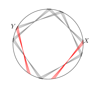
Figure 5. Graphing corresponding to an irrational rotation of the circle.

Given $N>0$, we can choose $X$ small enough so that

1. $T^{i}(X)\cap T^{j}(X)=\emptyset$, for $0\leq i<j\leq N$,
   

2. For $A:=X\sqcup T(X)\sqcup\cdots\sqcup T^{N}(X)$, $\mu_{H}(A)\leq\frac{1}{2}$.
   

Write $Y=T^{N}(X)$. The only edges that contribute to $e_{G}(A,A^{c})$ are the ones going from $Y$ to $T(Y)$ and the ones going from $T^{-1}(X)$ to $X$. These are shown in red in the above figure. Thus $e_{G}(A,A^{c})\leq 2\mu_{H}(X)$. Therefore we have

(7.4) $$h_{G}\leq h_{G}(A)\leq\frac{e_{G}(A,A^{c})}{\operatorname{vol}_{G}(A)}\leq 2\frac{\mu_{H}(A)}{(N+1)\mu_{H}(A)}=2/(N+1)$$

Since $N$ is arbitrary, we conclude that $h_{G}=0$.

Remark 7.6.

An example of a connected graphing $G$ with positive $\lambda(G)$ and hence (by Theorem 6.4) positive Cheeger constant $h_{G}$ has been described by Lovasz in [Lov12, Example 21.5] under the rubric of ‘expander graphings’.

7.3. A necessary and sufficient condition for connectedness of a graphon

In the special case that a graphon $W$ has degree of every vertex uniformly bounded below, we shall now proceed to give a necessary and sufficient condition in terms of the Cheeger constant for $W$ to be connected. This is analogous to the statement that a finite graph is connected if and only if its Cheeger constant is positive.

Proposition 7.7.

Let $\varepsilon>0$ and $W$ be a graphon such that the degree $d_{W}(x)\geq\varepsilon$ for all $x\in I$. Then $W$ is connected if and only if $h_{W}>0$.

We provide two proofs of the above result. The first is an application of Theorem 5.4 the Buser inequality for graphons and is essentially self-contained using some basic facts about compact operators. The second proof uses a structural lemma about connected graphons proved in [BBCR10].

Definition 7.8.

[Lim96, pg. 196] We say that $\lambda\in\mathbf{R}$ is an approximate eigenvalue of a bounded linear operator $T:H\to H$ of a Hilbert space $H$ if the image of $T-\lambda I$ is not bounded below.

Lemma 7.9.

[Lim96, Lemma 27.5(a)] For any bounded linear self-adjoint operator $T:H\to H$ on a Hilbert space $H$, we have that

(7.5) $$\inf_{x\in H:\ \|x\|=1}\langle Tx,x\rangle$$

is an approximate eigenvalue of $T$.

Lemma 7.10.

[Lim96, Lemma 28.4] If $T:H\to H$ is a compact operator then every approximate eigenvalue of $T$ is an actual eigenvalue of $T$.

Lemma 7.11.

Let $W$ be a connected graphon with $d_{W}$ bounded below by a positive real. Then the map $(1/d_{W})T_{W}:L^{2}(I,\nu)\to L^{2}(I,\nu)$ is a compact operator.

Proof.

Since $d_{W}$ is bounded below, it follows that $L^{2}(I,\mu_{L})$ and $L^{2}(I,\nu)$ have comparable norms. Therefore $I:L^{2}(I,\mu_{L})\to L^{2}(I,\nu)$ is a bounded linear isomorphism. The operator $T_{W}:L^{2}(I,\mu_{L})\to L^{2}(I,\mu_{L})$ is compact [Lov12, Section 7.5]. Since $d_{W}$ is bounded below, i.e.  $1/d_{W}$ is $L^{\infty}$, it follows that the operator $(1/d_{W})T_{W}:L^{2}(I,\mu_{L})\to L^{2}(I,\mu_{L})$ is also compact.

Take any bounded sequence $(f_{n})$ in $L^{2}(I,\nu)$. Then $(f_{n})$ is bounded in $L^{2}(I,\mu_{L})$ too because of comparability of norms. Since $(1/d_{W})T_{W}:L^{2}(I,\mu_{L})\to L^{2}(I,\mu_{L})$ is compact, there exists a subsequence $(f_{n_{k}})$ such that $(1/d_{W})(T_{W}f_{n_{k}})$ converges in $L^{2}(I,\mu_{L})$. Again, the comparability of norms give that $(1/d_{W})(T_{W}f_{n_{k}})$ converges in $L^{2}(I,\nu)$ as required. ∎

Note that for any graphon $W$, the Laplacian $\Delta_{W}:L^{2}(I,\nu)\to L^{2}(I,\nu)$ restricts to a linear operator $\Delta_{W}:{\textbf{1}}^{\perp}_{v}\to{\textbf{1}}^{\perp}_{v}$.

Proof.

of Proposition 7.7:
If $h_{W}>0$ then clearly $W$ is connected. So we need to prove the other direction. Let $W$ be a connected graphon with $d_{W}(x)\geq\varepsilon$ for all $x\in I$. Lemma 7.11 ensures that $(1/d_{W})T_{W}$ is a compact operator on $L^{2}(I,\nu)$ and it is easy to check that it restricts to a linear operator from ${\textbf{1}}^{\perp}_{v}$ to itself. Throughout we will think of $\Delta_{W}$ and $(1/d_{W})T_{W}$ as linear operators in ${\textbf{1}}^{\perp}_{v}$. Now by Lemma 5.18 $\lambda(W)$ is an approximate eigenvalue of $\Delta_{W}$. Thus the image of $\Delta_{W}-\lambda(W)I=(1-\lambda(W))I-(1/d_{W})T_{W}$ is not bounded below in ${\textbf{1}}^{\perp}_{v}$. Hence $1-\lambda(W)$ is an approximate eigenvalue of $(1/d_{W})T_{W}$. But $(1/d_{W})T_{W}:{\textbf{1}}^{\perp}_{v}\to{\textbf{1}}^{\perp}_{v}$ is a compact operator, and thus by Lemma 7.10 we have that $1-\lambda(W)$ is in fact an eigenvalue of $(1/d_{W})T_{W}$. Therefore $\lambda(W)$ is an eigenvalue of $\Delta_{W}$. Let $f\in{\textbf{1}}^{\perp}_{v}$ be nonzero such that $\Delta_{W}f=\lambda(W)f$. If $h_{W}$ were equal to $0$, then by the Buser inequality (Theorem 5.4) we have that $\lambda(W)=0$. Thus $\Delta_{W}f=0$, which is equivalent to saying that $df=0$. But as observed in the first paragraph of Section 5.2 we then have that $f$ is a constant function and hence the only way it can belong to ${\textbf{1}}^{\perp}_{v}$ is that $f=0$–a contradiction. ∎

Now we give the second proof of Proposition 7.7.

Definition 7.12.

[BBCR10] Let $W$ be a graphon and $0<a,b<1$ be real numbers. An $(a,b)$-cut in $W$ is a partition $\{A,A^{c}\}$ of $I$ with $a<\mu_{L}(A)<1-a$ such that $e_{W}(A,A^{c})\leq b$.

Note that a graphon is connected if and only if it admits no $(a,0)$-cut for any $0<a\leq 1/2$.

Lemma 7.13.

[BBCR10, Lemma 7] Let $W$ be a connected graphon and $0<a<1/2$. Then there is some $b>0$ such that $W$ admits no $(a,b)$-cut.

Alternate proof of Proposition 7.7 using Lemma 7.13:
Let $W$ be a graphon with $d_{W}(x)\geq\varepsilon$ for all $x$. We prove the non-trivial direction. Assume $W$ is connected. We will show that $h_{W}>0$. Assume on the contrary that $h_{W}=0$. Then for each $n\geq 1$ there is a measurable subset $A_{n}$ of $I$ with $0<\mu_{L}(A_{n})<1$ such that $h_{W}(A_{n})<1/n$. After passing to a subsequence, there are two cases to consider.

Case 1: $\mu_{L}(A_{n})\to 0$ as $n\to\infty$.

In this case we have for large $n$ that

(7.6) $$\begin{split}h_{W}(A_{n})&=\frac{e(A_{n},A_{n}^{c})}{\operatorname{vol}(A_{n})}=\frac{\operatorname{vol}(A_{n})-\int_{A_{n}\times A_{n}}W}{\operatorname{vol}(A_{n})}\\ &=1-\frac{\int_{A_{n}\times A_{n}}W}{\operatorname{vol}(A_{n})}\geq 1-\frac{\mu_{L}(A_{n})^{2}}{\varepsilon\mu_{L}(A_{n})}\\ &\geq 1-\mu_{L}(A_{n})/\varepsilon\end{split}$$

But this contradicts the assumption that $h_{W}(A_{n})<1/n$ for all $n$.

Case 2: $\mu_{L}(A_{n})\to t$ for some $t>0$.

Let $0<a<1/2$ be such that $a<t<1-a$. Now by Lemma 7.13, there is a $b>0$ such that $W$ admits no $(a,b)$-cut. Therefore for all $n$ large enough we have

(7.7) $$\begin{split}h_{W}(A_{n})&=\frac{e(A_{n},A_{n}^{c})}{\min\{\operatorname{vol}(A_{n}),\operatorname{vol}(A_{n}^{c})\}}\\ &\geq\frac{b}{\varepsilon\min\{\mu_{L}(A_{n}),\mu_{L}(A_{n}^{c})\}}\geq\frac{b}{\varepsilon(1-a)}\end{split}$$

which again contradicts the assumption that $h_{W}(A_{n})<1/n$ for all $n$. $\blacksquare$

References

- [Alo86] N. Alon. Eigenvalues and expanders. Combinatorica, 6(2):83–96, 1986. Theory of computing (Singer Island, Fla., 1984).
- [AM85] N. Alon and V. D. Milman. isoperimetric inequalities for graphs, and superconcentrators. J. Combin. Theory Ser. B, 38(1):73–88, 1985.
- [BBCR10] Béla Bollobás, Christian Borgs, Jennifer Chayes, and Oliver Riordan. Percolation on dense graph sequences. Ann. Probab., 38(1):150–183, 2010.
- [BCKL13] Christian Borgs, Jennifer Chayes, Jeff Kahn, and László Lovász. Left and right convergence of graphs with bounded degree. Random Structures Algorithms, 42(1):1–28, 2013.
- [BCL+08] C. Borgs, J. T. Chayes, L. Lovász, V. T. Sós, and K. Vesztergombi. Convergent sequences of dense graphs. I. Subgraph frequencies, metric properties and testing. Adv. Math., 219(6):1801–1851, 2008.
- [BCL+12] C. Borgs, J. T. Chayes, L. Lovász, V. T. Sós, and K. Vesztergombi. Convergent sequences of dense graphs II. Multiway cuts and statistical physics. Ann. of Math. (2), 176(1):151–219, 2012.
- [Bus10] Peter Buser. Geometry and spectra of compact Riemann surfaces. Modern Birkhäuser Classics. Birkhäuser Boston, Inc., Boston, MA, 2010. Reprint of the 1992 edition.
- [Cha84] Isaac Chavel. Eigenvalues in Riemannian geometry, volume 115 of Pure and Applied Mathematics. Academic Press, Inc., Orlando, FL, 1984. Including a chapter by Burton Randol, With an appendix by Jozef Dodziuk.
- [Cha17] Sourav Chatterjee. Large deviations for random graphs, volume 2197 of Lecture Notes in Mathematics. Springer, Cham, 2017. Lecture notes from the 45th Probability Summer School held in Saint-Flour, June 2015, École d’Été de Probabilités de Saint-Flour. [Saint-Flour Probability Summer School].
- [Che70] Jeff Cheeger. A lower bound for the smallest eigenvalue of the Laplacian. Problems in analysis (Papers dedicated to Salomon Bochner, 1969), pages 195–199, 1970.
- [Chu97] F. R. K. Chung. Spectral graph theory, volume 92 of CBMS Regional Conference Series in Mathematics. Published for the Conference Board of the Mathematical Sciences, Washington, DC; by the American Mathematical Society, Providence, RI, 1997.
- [Chu10] Fan Chung. Four proofs for the Cheeger inequality and graph partition algorithms. In Fourth International Congress of Chinese Mathematicians, volume 48 of AMS/IP Stud. Adv. Math., pages 331–349. Amer. Math. Soc., Providence, RI, 2010.
- [Dod84] Jozef Dodziuk. Difference equations, isoperimetric inequality and transience of certain random walks. Trans. Amer. Math. Soc., 284(2):787–794, 1984.
- [Ele08] Gábor Elek. Weak convergence of finite graphs, integrated density of states and a Cheeger type inequality. J. Combin. Theory Ser. B, 98(1):62–68, 2008.
- [EW11] Manfred Einsiedler and Thomas Ward. Ergodic theory with a view towards number theory, volume 259 of Graduate Texts in Mathematics. Springer-Verlag London, Ltd., London, 2011.
- [FN02] S. Friedland and R. Nabben. On Cheeger-type inequalities for weighted graphs. J. Graph Theory, 41(1):1–17, 2002.
- [Lim96] Balmohan V. Limaye. Functional analysis. New Age International Publishers Limited, New Delhi, second edition, 1996.
- [Lov12] Laszlo Lovász. Large networks and graph limits, volume 60 of American Mathematical Society Colloquium Publications. American Mathematical Society, Providence, RI, 2012.
- [Moh91] Bojan Mohar. The Laplacian spectrum of graphs. In Graph theory, combinatorics, and applications. Vol. 2 (Kalamazoo, MI, 1988), Wiley-Intersci. Publ., pages 871–898. Wiley, New York, 1991.
- [Tre11] Luca Trevisan. Graph partitioning and expanders. Course Notes, https://people.eecs.berkeley.edu/ luca/cs359g/lecture04.pdf, pages 331–349, 2011.