The price of debiasing automatic metrics in natural language evaluation
Abstract
For evaluating generation systems, automatic metrics such as BLEU cost nothing to run but have been shown to correlate poorly with human judgment, leading to systematic bias against certain model improvements. On the other hand, averaging human judgments, the unbiased gold standard, is often too expensive. In this paper, we use control variates to combine automatic metrics with human evaluation to obtain an unbiased estimator with lower cost than human evaluation alone. In practice, however, we obtain only a 7–13% cost reduction on evaluating summarization and open-response question answering systems. We then prove that our estimator is optimal: there is no unbiased estimator with lower cost. Our theory further highlights the two fundamental bottlenecks—the automatic metric and the prompt shown to human evaluators—both of which need to be improved to obtain greater cost savings.
1 Introduction
In recent years, there has been an increasing interest in tasks that require generating natural language, including abstractive summarization (Nallapati et al., 2016), open-response question answering (Nguyen et al., 2016; Kočisky et al., 2017), image captioning (Lin et al., 2014), and open-domain dialogue (Lowe et al., 2017b). Unfortunately, the evaluation of these systems remains a thorny issue because of the diversity of possible correct responses. As the gold standard of performing human evaluation is often too expensive, there has been a large effort developing automatic metrics such as BLEU (Papineni et al., 2002), ROUGE (Lin and Rey, 2004), METEOR (Lavie and Denkowski, 2009; Denkowski and Lavie, 2014) and CiDER (Vedantam et al., 2015). However, these have shown to be biased, correlating poorly with human metrics across different datasets and systems (Liu et al., 2016b; Novikova et al., 2017).
Can we combine automatic metrics and human evaluation to obtain an unbiased estimate at lower cost than human evaluation alone? In this paper, we propose a simple estimator based on control variates (Ripley, 2009), where we average differences between human judgments and automatic metrics rather than averaging the human judgments alone. Provided the two are correlated, our estimator will have lower variance and thus reduce cost.
We prove that our estimator is optimal in the sense that no unbiased estimator using the same automatic metric can have lower variance. We also analyze its data efficiency (equivalently, cost savings)—the factor reduction in number of human judgments needed to obtain the same accuracy versus naive human evaluation—and show that it depends solely on two factors: (a) the annotator variance (which is a function of the human evaluation prompt) and (b) the correlation between human judgments and the automatic metric. This factorization allows us to calculate typical and best-case data efficiencies and accordingly refine the evaluation prompt or automatic metric.
Finally, we evaluate our estimator on state-of-the-art systems from two tasks, summarization on the CNN/Daily Mail dataset Hermann et al. (2015); Nallapati et al. (2016) and open-response question answering on the MS MARCOv1.0 dataset (Nguyen et al., 2016). To study our estimators offline, we preemptively collected 10,000 human judgments which cover several tasks and systems.111An anonymized version of this data and the annotation interfaces used can be found at https://bit.ly/price-of-debiasing. As predicted by the theory, we find that the data efficiency depends not only on the correlation between the human and automatic metrics, but also on the evaluation prompt. If the automatic metric had perfect correlation, our data efficiency would be around 3, while if we had noiseless human judgments, our data efficiency would be about 1.5. In reality, the reduction in cost we obtained was only about 10%, suggesting that improvements in both automatic metric and evaluation prompt are needed. As one case study in improving the latter, we show that, when compared to a Likert survey, measuring the amount of post-editing needed to fix a generated sentence reduced the annotator variance by three-fold.
2 Bias in automatic evaluation
| Question and reference answer | System answer (System; Corr / ROUGE-L) |
|---|---|
| Examples where system is correct and ROUGE-L ( or 285 of 1455 unique responses) | |
| Q. what is anti-mullerian hormone A. Anti-Mullerian Hormone (AMH) is a protein hormone produced by granulosa cells (cells lining the egg sacs or follicles) within the ovary. | it is a protein hormone produced by granulosa cells (cells lining the egg sacs or follicles) within the ovary. (snet.ens; / ) |
| Examples where system is incorrect and ROUGE-L ( or 19 of 1455 unique responses) | |
| Q. at what gestational age can you feel a fetus move A. 37 to 41 weeks (incorrect reference answer) | 37 to 41 weeks (fastqa, fastqa.ext; / 1.0) |
| Examples where system is correct and ROUGE-L ( or 815 of 1455 unique responses) | |
| Q. what is the definition of onomatopoeia A. It is defined as a word, which imitates the natural sounds of a thing. | the naming of a thing or action by a vocal imitation of the sound associated with it (as buzz, hiss). (fastqa; / ) |
| Examples where system is incorrect and ROUGE-L ( or 336 of 1455 unique responses) | |
| Q. what kind root stem does a dandelion have A. Fibrous roots and hollow stem. | vitamin a, vitamin c, vitamin d and vitamin b complex, as well as zinc, iron and potassium. (snet, snet.ens; / ) |
| Reference summary | System summary (System; Edit / VecSim) |
|---|---|
| Examples where system Edit and VecSim ( or 1078 of 2000 responses) | |
| Bhullar is set to sign a -day contract with the Kings. The -year-old will become the NBA’s first player of Indian descent. Bhullar will be on the roster when the Kings host New Orleans Pelicans. | Bhullar andThe Kings are signing Bhullar to a -day contract. The -year-old will be on the roster on friday when David Wear’s -season contract expires thursday. Bhullar is set to become the NBA’s first player of Indian descent. (ml; / ) |
| Examples where system Edit and VecSim ( or 360 of 2000 responses) | |
| The Direct Marketing Commission probing B2C Data and Data Bubble. Investigating whether they breached rules on the sale of private data. Chief commissioner described allegations made about firms as ‘serious’. | Data obtained by the Mail’s marketing commission said it would probe both companies over claims that they had breached the rules on the sale of private data. The FSA said it would probe both companies over claims they had breached the rules on the sale of private data. (se2seq; / ) |
| Examples where system Edit and VecSim ( or 290 of 2000 responses) | |
| Death toll rises to more than . Pemba Tamang, , shows no apparent signs of serious injury after rescue. Americans special forces helicopter , including Americans, to safety. | Six of Despite Nepal’s tragedy, life triumphed in Kathmandu’s hard-hit neighborhoods. Rescuers pulled an 15-year-old from the rubble of a multistory residential building. He was wearing a New York shirt and a blue neck brace. (pointer; / ) |
| Examples where system Edit and VecSim ( or 272 of 2000 responses) | |
| “Mad Men’s” final seven episodes begin airing April . The show has never had high ratings but is considered one of the great TV series. It’s unknown what will happen to characters, but we can always guess. | ‘This’s “Mad Men” is the end of a series of an era’, This he says. Stores have created fashion lines inspired by the show.“The Sopranos”. The in the Kent State shootings in may or Richard Nixonś re-election.. (ml+rl; / ) |
It is well understood that current automatic metrics tend to correlate poorly with human judgment at the instance-level. For example, Novikova et al. (2017) report correlations less than for a large suite of word-based and grammar-based evaluation methods on a generation task. Similarly, Liu et al. (2016b) find correlations less than for automatic metrics on a dialog generation task in one domain, but find correlations with the same metric dropped significantly to less than when used in another domain. Still, somewhat surprisingly, several automatic metrics have been found to have high system-level correlations (Novikova et al., 2017). What, then, are the implications of having a low instance-level correlation?
As a case study, consider the task of open-response question answering: here, a system receives a human-generated question and must generate an answer from some given context, e.g. a document or several webpages. We collected the responses of several systems on the MS MARCOv1 dataset (Nguyen et al., 2016) and crowdsourced human evaluations of the system output (see Section 4 for details).
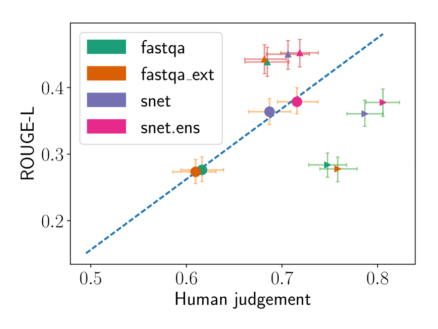
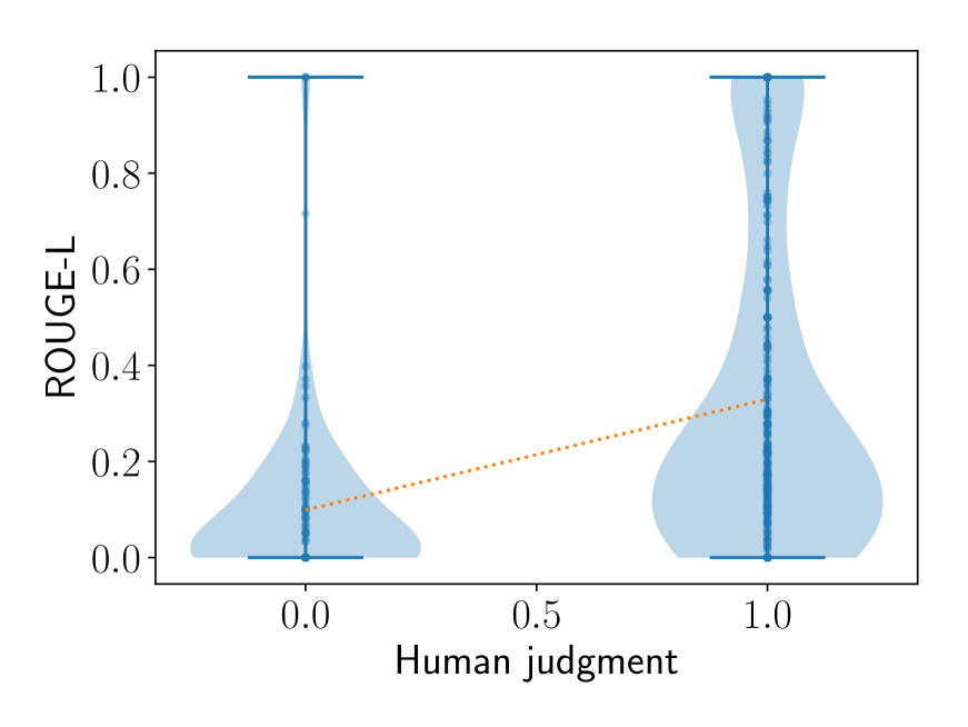
The instance-level correlation (Figure 1(b)) is only . A closer look at the instance-level correlation reveals that while ROUGE is able to correctly assign low scores to bad examples (lower left), it is bad at judging good examples and often assigns them low ROUGE scores (lower right)—see Table 1 for examples. This observation agrees with a finding reported in Novikova et al. (2017) that automatic metrics correlate better with human judgments on bad examples than average or good examples.
Thus, as Figure 1(a) shows, we can improve low-scoring ROUGE examples without improving their human judgment () and vice versa (). Indeed, Conroy and Dang (2008) report that summarization systems were optimized for ROUGE during the DUC challenge (Dang, 2006) until they were indistinguishable from the ROUGE scores of human-generated summaries, but the systems had hardly improved on human evaluation. Hill-climbing on ROUGE can also lead to a system that does worse on human scores, e.g. in machine translation (Wu et al., 2016). Conversely, genuine quality improvements might not be reflected in improvements in ROUGE. This bias also appears in pool-based evaluation for knowledge base population (Chaganty et al., 2017). Thus the problems with automatic metrics clearly motivate the need for human evaluation, but can we still use the automatic metrics somehow to save costs?
3 Statistical estimation for unbiased evaluation
We will now formalize the problem of combining human evaluation with an automatic metric. Let be a set of inputs (e.g., articles), and let be the system (e.g. for summarization), which takes and returns output (e.g. a summary). Let be the set of system predictions. Let be the random variable representing the human judgment according to some evaluation prompt (e.g. grammaticality or correctness), and define to be the (unknown) human metric corresponding to averaging over an infinite number of human judgments. Our goal is to estimate the average across all examples:
| (1) |
with as few queries to as possible.
Let be an automatic metric (e.g. ROUGE), which maps to a real number. We assume evaluating is free. The central question is how to use in conjunction with calls to to produce an unbiased estimate (that is, ). In this section, we will construct a simple estimator based on control variates (Ripley, 2009), and prove that it is minimax optimal.
3.1 Sample mean
We warm up with the most basic unbiased estimate, the sample mean. We sample independently with replacement from . Then, we sample each human judgment independently.222Note that this independence assumption isn’t quite true in practice since we do not control who annotates our data. Define the estimator to be . Note that is unbiased ().
We can define as the variance of the human metric and as the variance of human judgment averaged over . By the law of total variance, the variance of our estimator is
| (2) |
3.2 Control variates estimator
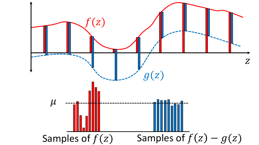
Now let us see how an automatic metric can reduce variance. If there is no annotator variance () so that , we should expect the variance of to be lower than the variance of , assuming is correlated with —see Figure 2 for an illustration.
The actual control variates estimator needs to handle noisy (i.e. ) and guard against a with low correlation. Let us standardize to have zero mean and unit variance, because we have assumed it is free to evaluate. As before, let be independent samples from and draw independently as well. We define the control variates estimator as
| (3) |
where
| (4) |
Intuitively, we have averaged over to handle the noise introduced by , and scaled to prevent an uncorrelated automatic metric from introducing too much noise.
An important quantity governing the quality of an automatic metric is the correlation between and (recall that has unit variance):
| (5) |
We can show that among all distributions with fixed , , and (equivalently ), this estimator is minimax optimal, i.e. it has the least variance among all unbiased estimators:
Theorem 3.1.
Among all unbiased estimators that are functions of and , and for all distributions with a given , , and ,
| (6) |
and no other estimator has a lower worst-case variance.
Comparing the variances of the two estimators ((2) and (6)), we define the data efficiency as the ratio of the variances:
| (7) |
where is the normalized annotator variance. Data efficiency is the key quantity in this paper: it is the multiplicative reduction in the number of samples required when using the control variates estimator versus the sample mean . Figure 3 shows the inverse data efficiency contours as a function of the correlation and .
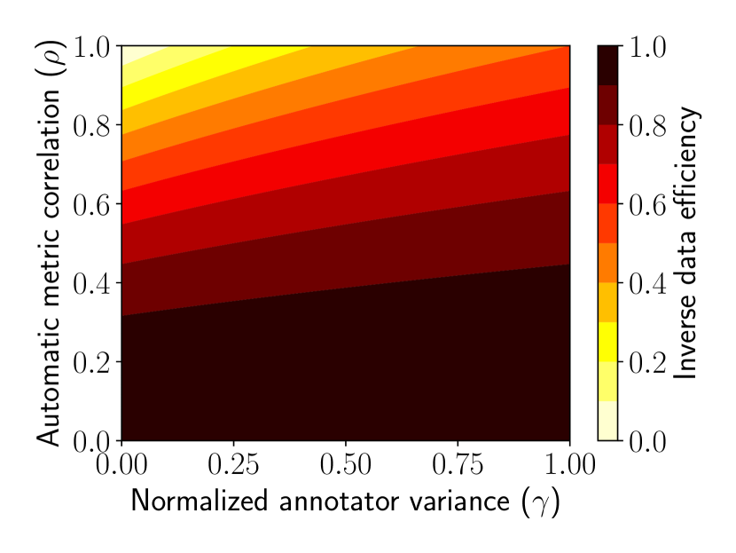
When there is no correlation between human and automatic metrics (), the data efficiency is naturally (no gain). In order to achieve a data efficiency of (half the labeling cost), we need . Interestingly, even for an automatic metric with perfect correlation (), the data efficiency is still capped by : unless the data efficiency cannot increase unboundedly. Intuitively, even if we knew that , would be undetermined up to a constant additive shift and just estimating the shift would incur a variance of .
3.3 Using the control variates estimator
The control variates estimator can be easily integrated into an existing evaluation: we run human evaluation on a random sample of system outputs, automatic evaluation on all the system outputs, and plug in these results into Algorithm 1.
It is vital that we are able to evaluate the automatic metric on a significantly larger set of examples than those with human evaluations to reliably normalize : without these additional examples, it be can shown that the optimal minimax estimator for is simply the naive estimate . Intuitively, this is because estimating the mean of incurs an equally large variance as estimating . In other words, is only useful if we have additional information about beyond the samples .
Algorithm 1 shows the estimator. In practice, we do not know , so we use a plug-in estimate in line 3 to compute the estimate in line 4. We note that estimating from data does introduce a bias, but when compared to the standard deviation which decays as , this bias quickly goes to .
Proposition 3.1.
The estimator in Algorithm 1 has bias.
An additional question that arises when applying Algorithm 1 is figuring out how many samples to use. Given a target variance, the number of samples can be estimated using (6) with conservative estimates of , and . Alternatively, our estimator can be combined with a dynamic stopping rule (Mnih et al., 2008) to stop data collection once we reach a target confidence interval.
3.4 Discussion of assumptions
We will soon see that empirical instantiations of and lead to rather underwhelming data efficiencies in practice. In light of our optimality result, does this mean there is no hope for gains? Let us probe our assumptions. We assumed that the human judgments are uncorrelated across different system outputs; it is possible that a more accurate model of human annotators (e.g. Passonneau and Carpenter (2014)) could offer improvements. Perhaps with additional information about such as calibrated confidence estimates, we would be able to sample more adaptively. Of course the most direct routes to improvement involve increasing the correlation of with human judgments and reducing annotator variance, which we will discuss more later.
| Task | Eval. | |||
|---|---|---|---|---|
| CDM | Fluency | 0.32 | 0.26 | 1.23 |
| CDM | Redund. | 0.26 | 0.43 | 0.61 |
| CDM | Overall | 0.28 | 0.28 | 1.00 |
| CDM | Edit | 0.07 | 0.18 | 0.36 |
| MS MARCO | AnyCorr. | 0.14 | 0.15 | 0.95 |
| MS MARCO | AvgCorr. | 0.12 | 0.13 | 0.91 |
4 Tasks and datasets
In order to compare different approaches to evaluating systems, we first collected human judgments for the output of several automatic summarization and open-response question answering systems using Amazon Mechanical Turk. Details of instructions provided and quality assurance steps taken are provided in Appendix A of the supplementary material. In this section, we’ll briefly describe how we collected this data.
Evaluating language quality in automatic summarization.
In automatic summarization, systems must generate a short (on average two or three sentence) summary of an article: for our study, we chose articles from the CNN/Daily Mail (CDM) dataset (Hermann et al., 2015; Nallapati et al., 2016) which come paired with reference summaries in the form of story highlights. We focus on the language quality of summaries and leave evaluating content selection to future work.
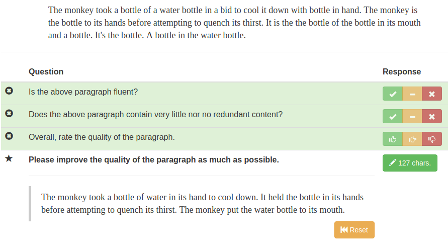
For each summary, we collected human judgments on a scale from 1–3 (Figure 4(a)) for fluency, (lack of) redundancy, and overall quality of the summary using guidelines from the DUC summarization challenge (Dang, 2006). As an alternate human metric, we also asked workers to post-edit the system’s summary to improve its quality, similar to the post-editing step in MT evaluations (Snover et al., 2006). Obtaining judgments costs about $0.15 per summary and this cost rises to about $0.40 per summary for post-editing.
We collected judgments on the summaries generated by the seq2seq and pointer models of See et al. (2017), the ml and ml+rl models of Paulus et al. (2018), and the reference summaries.333All system output was obtained from the original authors through private communication. Before presenting the summaries to human annotators, we performed some minimal post-processing: we true-cased and de-tokenized the output of seq2seq and pointer using Stanford CoreNLP (Manning et al., 2014) and replaced “unknown” tokens in each system with a special symbol ().
Evaluating answer correctness.
Next, we look at evaluating the correctness of system outputs in question answering using the MS MARCO question answering dataset (Nguyen et al., 2016). Here, each system is provided with a question and up to 10 paragraphs of context. The system generates open-response answers that do not need to be tied to a span in any paragraph.
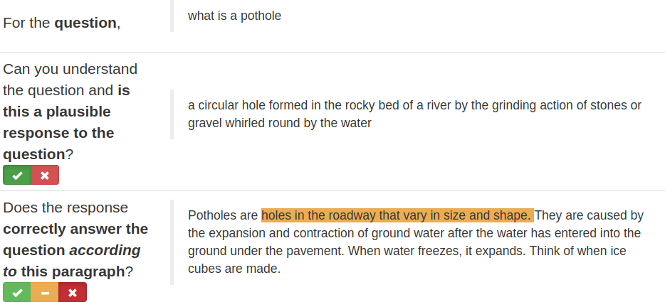
We first ask annotators to judge if the output is even plausible for the question, and if yes, ask them identify if it is correct according to each context paragraph. We found that requiring annotators to highlight regions in the text that support their decision substantially improved the quality of the output without increasing costs. Annotations cost $0.40 per system response.444This cost could be significantly reduced if systems also specify which passage they used to generate the answer.
While our goal is to evaluate the correctness of the provided answer, we found that there are often answers which may be correct or incorrect depending on the context. For example, the question “what is a pothole” is typically understood to refer to a hole in a roadway, but also refers to a geological feature (Figure 4(b)). This is reflected when annotators mark one context paragraph to support the given answer but mark another to contradict it. We evaluated systems based on both the average correctness (AvgCorrect) of their answers across all paragraphs as well as whether their answer is correct according to any paragraph (AnyCorrect).
We collected annotations on the systems generated by the fastqa and fastqa_ext from Weissenborn et al. (2017) and the snet and snet.ens(emble) models from Tan et al. (2018), along with reference answers. The answers generated by the systems were used without any post-processing. Surprisingly, we found that the correctness of the reference answers (according to the AnyCorrect metric) was only 73.5%, only 2% above that of the leading system (snet.ens). We manually inspected 30 reference answers which were annotated incorrectly and found that of those, about 95% were indeed incorrect. However, 62% are actually answerable from some paragraph, indicating that the real ceiling performance on this dataset is around 90% and that there is still room for improvement on this task.
5 Experimental results
We are now ready to evaluate the performance of our control variates estimator proposed in Section 3 using the datasets presented in Section 4. Recall that our primary quantity of interest is data efficiency, the ratio of the number of human judgments required to estimate the overall human evaluation score for the control variates estimator versus the sample mean. We’ll briefly review the automatic metrics used in our evaluation before analyzing the results.
Automatic metrics.
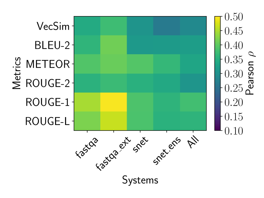
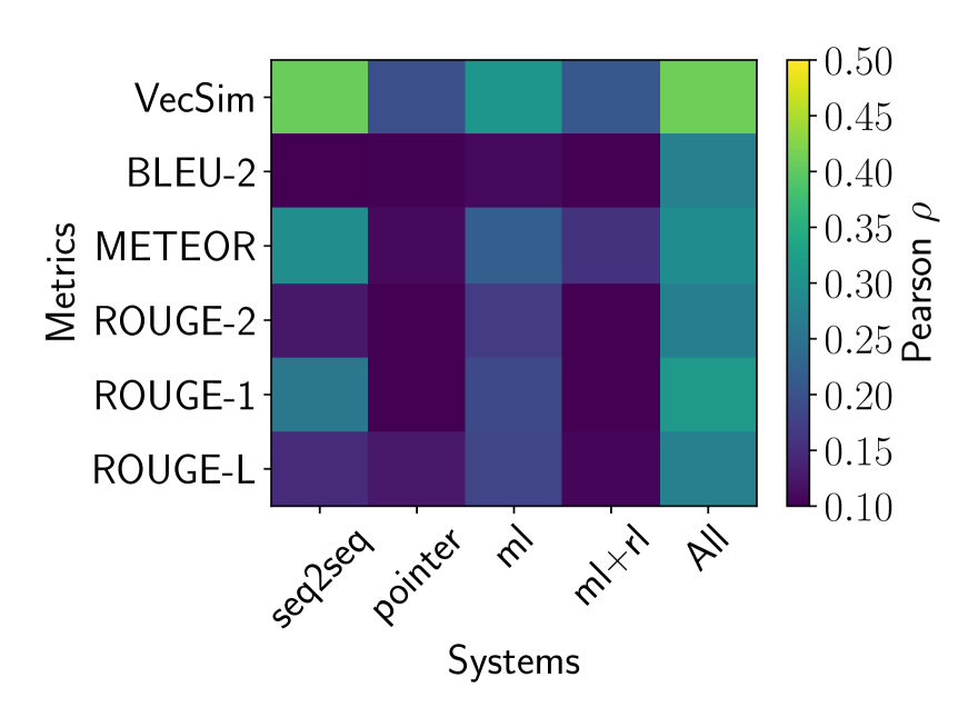
We consider the following frequently used automatic word-overlap based metrics in our work: BLEU (Papineni et al., 2002), ROUGE (Lin and Rey, 2004) and METEOR (Lavie and Denkowski, 2009). Following Novikova et al. (2017) and Liu et al. (2016b), we also compared a vector-based sentence-similarity using sent2vec (Pagliardini et al., 2017) to compare sentences (VecSim). Figure 5 shows how each of these metrics is correlated with human judgment for the systems being evaluated. Unsurprisingly, the correlation varies considerably across systems, with token-based metrics correlating more strongly for systems that are more extractive in nature (fastqa and fastqa_ext).
Results.555Extended results for other systems, metrics and prompts can be found at https://bit.ly/price-of-debiasing/.
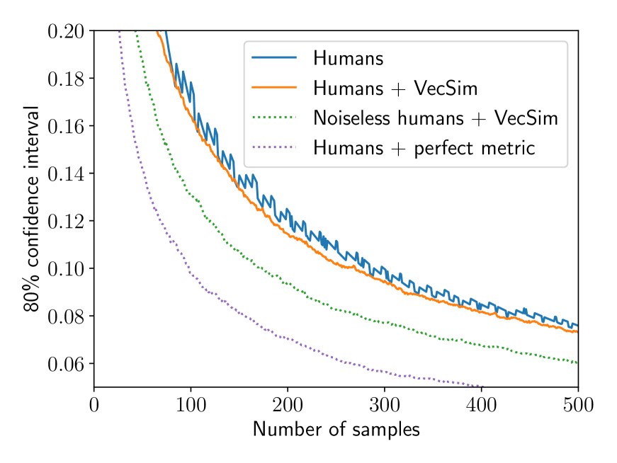
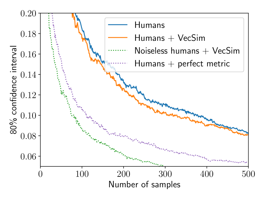
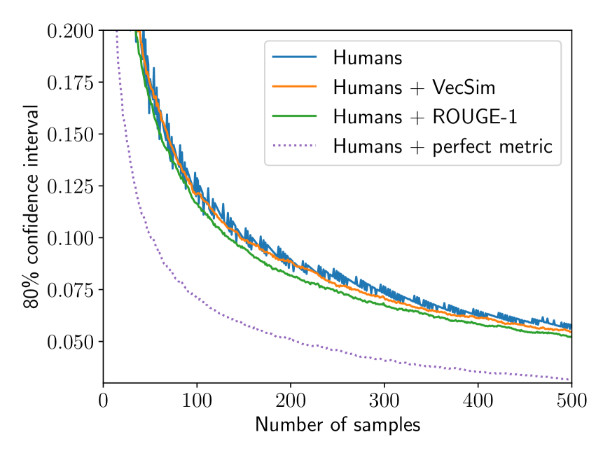
In Section 3 we proved that the control variates estimator is not only unbiased but also has the least variance among other unbiased estimators. Figure 6 plots the width of the 80% confidence interval, estimated using bootstrap, measured as a function of the number of samples collected for different tasks and prompts. As expected, the control variates estimator reduces the width of the confidence interval. We measure data efficiency by the averaging of the ratio of squared confidence intervals between the human baseline and control variates estimates. We observe that the data efficiency depends on the task, prompt and system, ranging from about 1.08 (a 7% cost reduction) to 1.15 (a 13% cost reduction) using current automatic metrics.
As we showed in Section 3, further gains are fundamentally limited by the quality of the evaluation prompts and automatic metrics. Figures 6(a) and 6(b) show how improving the quality of the evaluation prompt from a Likert-scale prompt for quality (Overall) to using post-editing (Edit) noticeably decreases variance and hence allows better automatic metrics to increase data efficiency. Likewise, Figure 6(c) shows how using a better automatic metric (ROUGE-L instead of VecSim) also reduces variance.
Figure 6 also shows the conjectured confidence intervals if we were able to eliminate noise in human judgments (noiseless humans) or have a automatic metric that correlated perfectly with average human judgment (perfect metric). In particular, we use the mean of all (2–3) humans on each for the perfect and use the mean of all humans on each for the “noiseless” .
In both cases, we are able to significantly increase data efficiency (i.e. decrease estimator variance). With zero annotator variance and using existing automatic metrics, the data efficiency ranges from 1.42 to 1.69. With automatic metrics with perfect correlation and current variance of human judgments, it ranges from 2.38 to 7.25. Thus, we conclude that it is important not only to improve our automatic metrics but also the evaluation prompts we use during human evaluation.
6 Related work
In this work, we focus on using existing automatic metrics to decrease the cost of human evaluations. There has been much work on improving the quality of automatic metrics. In particular, there is interest in learning models (Lowe et al., 2017a; Dusek et al., 2017) that are able to optimize for improved correlations with human judgment. However, in our experience, we have found that these learned automatic metrics have trouble generalizing to different systems. The framework we provide allows us to safely incorporate such models into evaluation, exploiting them when their correlation is high but also not introducing bias when it is low.
Our key technical tool is control variates, a standard statistical technique used to reduce the variance of Monte Carlo estimates (Ripley, 2009). The technique has also been used in machine learning and reinforcement learning to lower variance estimates of gradients (Greensmith et al., 2004; Paisley et al., 2012; Ranganath et al., 2014). To the best of our knowledge, we are the first to apply this technique in the context of language evaluation.
Our work also highlights the importance of human evaluation. Chaganty et al. (2017) identified a similar problem of systematic bias in evaluation metrics in the setting of knowledge base population and also propose statistical estimators that relies on human evaluation to correct bias. Unfortunately, their technique relies on having a structured output (relation triples) that are shared between systems and does not apply to evaluating natural language generation. In a similar vein, Chang et al. (2017) dynamically collect human feedback to learn better dialog policies.
7 Discussion
Prior work has shown that existing automatic metrics have poor instance-level correlation with mean human judgment and that they score many good quality responses poorly. As a result, the evaluation is systematically biased against genuine system improvements that would lead to higher human evaluation scores but not improve automatic metrics. In this paper, we have explored using an automatic metric to decrease the cost of human evaluation without introducing bias. In practice, we find that with current automatic metrics and evaluation prompts data efficiencies are only 1.08–1.15 (7–13% cost reduction). Our theory shows that further improvements are only possible by improving the correlation of the automatic metric and reducing the annotator variance of the evaluation prompt. As an example of how evaluation prompts could be improved, we found that using post-edits of summarizes decreased normalized annotator variance by a factor of three relative to using a Likert scale survey. It should be noted that changing the evaluation prompt also changes the underlying ground truth : it is up to us to find a prompt that still captures the essence of what we want to measure.
Without making stronger assumptions, the control variates estimator we proposed outlines the limitations of unbiased estimation. Where do we go from here? Certainly, we can try to improve the automatic metric (which is potentially as difficult as solving the task) and brainstorming alternative ways of soliciting evaluation (which has been less explored). Alternatively, we could give up on measuring absolute scores, and seek instead to find techniques stably rank methods and thus improve them. As the NLP community tackles increasingly difficult tasks, human evaluation will only become more important. We hope our work provides some clarity on to how to make it more cost effective.
Reproducibility
All code, data, and experiments for this paper are available on the CodaLab platform at https://bit.ly/price-of-debiasing.
Acknowledgments
We are extremely grateful to the authors of the systems we evaluated for sharing their systems’ output with us. We also would like to thank Urvashi Khandelwal and Peng Qi for feedback on an earlier draft of the paper, the crowdworkers on Amazon Mechanical Turk and TurkNation for their work and feedback during the data collection process, and the anonymous reviewers for their constructive feedback.
References
- Chaganty et al. (2017) A. Chaganty, A. Paranjape, P. Liang, and C. Manning. 2017. Importance sampling for unbiased on-demand evaluation of knowledge base population. In Empirical Methods in Natural Language Processing (EMNLP).
- Chang et al. (2017) C. Chang, R. Yang, L. Chen, X. Zhou, and K. Yu. 2017. Affordable on-line dialogue policy learning. In Empirical Methods in Natural Language Processing (EMNLP). pages 223–231.
- Conroy and Dang (2008) J. M. Conroy and H. T. Dang. 2008. Mind the gap : Dangers of divorcing evaluations of summary content from linguistic quality. In International Conference on Computational Linguistics (COLING). pages 145–152.
- Dang (2006) H. T. Dang. 2006. Overview of DUC 2006. In Document Understanding Conference.
- Denkowski and Lavie (2014) M. Denkowski and A. Lavie. 2014. Meteor universal: Language specific translation evaluation for any target language. In Workshop on Statistical Machine Translation.
- Dusek et al. (2017) O. Dusek, J. Novikova, and V. Rieser. 2017. Referenceless quality estimation for natural language generation. arXiv .
- Greensmith et al. (2004) E. Greensmith, P. L. Bartlett, and J. Baxter. 2004. Variance reduction techniques for gradient estimates in reinforcement learning. Journal of Machine Learning Research (JMLR) 5:1471–1530.
- Hermann et al. (2015) K. M. Hermann, T. Kočiský, E. Grefenstette, L. Espeholt, W. Kay, M. Suleyman, and P. Blunsom. 2015. Teaching machines to read and comprehend. In Advances in Neural Information Processing Systems (NIPS).
- Kočisky et al. (2017) T. Kočisky, J. Schwarz, P. Blunsom, C. Dyer, K. M. Hermann, G. Melis, and E. Grefenstette. 2017. The NarrativeQA reading comprehension challenge. arXiv preprint arXiv:1712.07040 .
- Lavie and Denkowski (2009) A. Lavie and M. Denkowski. 2009. The meteor metric for automatic evaluation of machine translation. Machine Translation 23.
- Lin and Rey (2004) C. Lin and M. Rey. 2004. Looking for a few good metrics: ROUGE and its evaluation. In NTCIR Workshop.
- Lin et al. (2014) T. Lin, M. Maire, S. Belongie, J. Hays, P. Perona, D. Ramanan, P. Doll’ar, and C. L. Zitnick. 2014. Microsoft COCO: Common objects in context. In European Conference on Computer Vision (ECCV). pages 740–755.
- Liu et al. (2016a) A. Liu, S. Soderland, J. Bragg, C. H. Lin, X. Ling, and D. S. Weld. 2016a. Effective crowd annotation for relation extraction. In North American Association for Computational Linguistics (NAACL). pages 897–906.
- Liu et al. (2016b) C. Liu, R. Lowe, I. V. Serban, M. Noseworthy, L. Charlin, and J. Pineau. 2016b. How NOT to evaluate your dialogue system: An empirical study of unsupervised evaluation metrics for dialogue response generation. In Empirical Methods in Natural Language Processing (EMNLP).
- Lowe et al. (2017a) R. Lowe, M. Noseworthy, I. V. Serban, N. Angelard-Gontier, Y. Bengio, and J. Pineau. 2017a. Towards an automatic turing test: Learning to evaluate dialogue responses. In Association for Computational Linguistics (ACL).
- Lowe et al. (2017b) R. T. Lowe, N. Pow, I. Serban, L. Charlin, C. Liu, and J. Pineau. 2017b. Training end-to-end dialogue systems with the ubuntu dialogue corpus. Dialogue and Discourse 8.
- Manning et al. (2014) C. D. Manning, M. Surdeanu, J. Bauer, J. Finkel, S. J. Bethard, and D. McClosky. 2014. The stanford coreNLP natural language processing toolkit. In ACL system demonstrations.
- Mnih et al. (2008) V. Mnih, C. Szepesv’ari, and J. Audibert. 2008. Empirical berstein stopping. In International Conference on Machine Learning (ICML).
- Nallapati et al. (2016) R. Nallapati, B. Zhou, C. Gulcehre, B. Xiang, et al. 2016. Abstractive text summarization using sequence-to-sequence rnns and beyond. arXiv preprint arXiv:1602.06023 .
- Nguyen et al. (2016) T. Nguyen, M. Rosenberg, X. Song, J. Gao, S. Tiwary, R. Majumder, and L. Deng. 2016. MS MARCO: A human generated machine reading comprehension dataset. In Workshop on Cognitive Computing at NIPS.
- Novikova et al. (2017) J. Novikova, O. Dušek, A. C. Curry, and V. Rieser. 2017. Why we need new evaluation metrics for NLG. In Empirical Methods in Natural Language Processing (EMNLP).
- Pagliardini et al. (2017) M. Pagliardini, P. Gupta, and M. Jaggi. 2017. Unsupervised learning of sentence embeddings using compositional n-gram features. arXiv .
- Paisley et al. (2012) J. Paisley, D. M. Blei, and M. I. Jordan. 2012. Variational Bayesian inference with stochastic search. In International Conference on Machine Learning (ICML). pages 1363–1370.
- Papineni et al. (2002) K. Papineni, S. Roukos, T. Ward, and W. Zhu. 2002. BLEU: A method for automatic evaluation of machine translation. In Association for Computational Linguistics (ACL).
- Passonneau and Carpenter (2014) R. J. Passonneau and B. Carpenter. 2014. The benefits of a model of annotation. In Association for Computational Linguistics (ACL).
- Paulus et al. (2018) R. Paulus, C. Xiong, and R. Socher. 2018. A deep reinforced model for abstractive summarization. In International Conference on Learning Representations (ICLR).
- Ranganath et al. (2014) R. Ranganath, S. Gerrish, and D. Blei. 2014. Black box variational inference. In Artificial Intelligence and Statistics (AISTATS). pages 814–822.
- Ripley (2009) B. D. Ripley. 2009. Stochastic simulation. John Wiley & Sons.
- See et al. (2017) A. See, P. J. Liu, and C. D. Manning. 2017. Get to the point: Summarization with pointer-generator networks. In Association for Computational Linguistics (ACL).
- Snover et al. (2006) M. Snover, B. Dorr, R. Schwartz, L. Micciulla, and J. Makhoul. 2006. A study of translation edit rate with targeted human annotation. In Association for Machine Translation in the Americas. pages 223–231.
- Tan et al. (2018) C. Tan, F. Wei, N. Yang, W. Lv, and M. Zhou. 2018. S-Net: From answer extraction to answer generation for machine reading comprehension. In Association for the Advancement of Artificial Intelligence (AAAI).
- Vedantam et al. (2015) R. Vedantam, C. L. Zitnick, and D. Parikh. 2015. CIDEr: Consensus-based image description evaluation. In Computer Vision and Pattern Recognition (CVPR). pages 4566–4575.
- Weissenborn et al. (2017) D. Weissenborn, G. Wiese, and L. Seiffe. 2017. Making neural QA as simple as possible but not simpler. In Computational Natural Language Learning (CoNLL).
- Wu et al. (2016) Y. Wu, M. Schuster, Z. Chen, Q. V. Le, M. Norouzi, W. Macherey, M. Krikun, Y. Cao, Q. Gao, K. Macherey, et al. 2016. Google’s neural machine translation system: Bridging the gap between human and machine translation. arXiv preprint arXiv:1609.08144 .
Appendix A Crowdsourcing data collection
In this section, we provide details regarding our the design of our annotation interfaces and the quality control measures we took.
A.1 Language quality evaluation.
Each human annotator was shown a short summary that was generated by a system from an article in the CNN/Daily Mail dataset or provided as a reference for that article. The annotators were then asked to (a) provide Likert scale ratings of the summary on multiple facets (fluency, redundancy and overall quality) and (b) perform post-edits to correct any errors (Figure 7(a)).
Interface design choices.
We found that using a five-level Likert scale increased annotator variance as annotators relative to a three-level Likert scale. Annotators were provided specific cues to calibrate their Likert ratings through a tutorial and were reminded of these cues through tooltips on the rating buttons (see Figure 7(b) for an example). If the annotators rated a summary as lacking along any facet, they were then forced to perform post-edits to “improve [its] quality as much as possible”. We found that forcing annotators to provide post-edits on examples significantly decreased the annotator variance even on the Likert ratings.

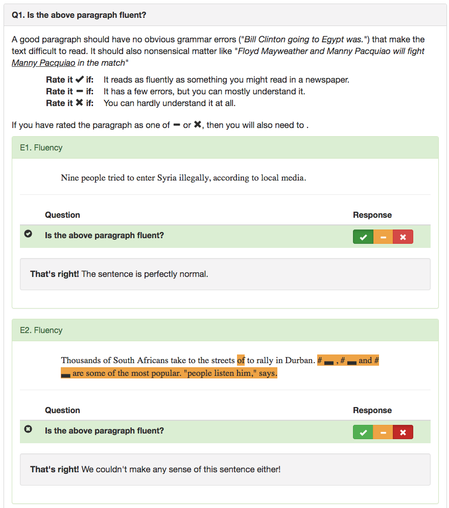
Following the recommendations of Liu et al. (2016a), we forced annotators to complete an interactive tutorial containing 10 questions each before beginning the task (Figure 7(b)). The tutorial provided guidelines and examples on how to rate each facet (fluency, redundancy and overall quality) and tested whether they were able to identify and correct language errors using the post-editing interface. The tutorial took about 5–6 minutes to complete and annotators were paid a one-time bonus of $0.75 on completion.
We initially included additional questions to assess focus, coherency and referential clarity adapted from the DUC evaluation guidelines (Dang, 2006), but found that annotators were unable to reliably identify these errors in the short summaries. We also experimented with asking annotators to highlight language errors in the text to justify their ratings, but again found that annotators were unable to localize these errors reliably.
Quality control measures.
We initially attempted to use attention-check examples for the Likert rating questions, but found that the ratings on these examples were themselves quite subjective and hence were not a reliable signal to reject work. Instead, we found that requiring post-edits to summaries significantly reduced spam. Additionally, we rejected annotators who took too little time to complete the task, had very low agreement rates on the Likert questions or had edits that were consistently shorter than 5 characters to prevent spam.
A.2 Answer correctness evaluation.
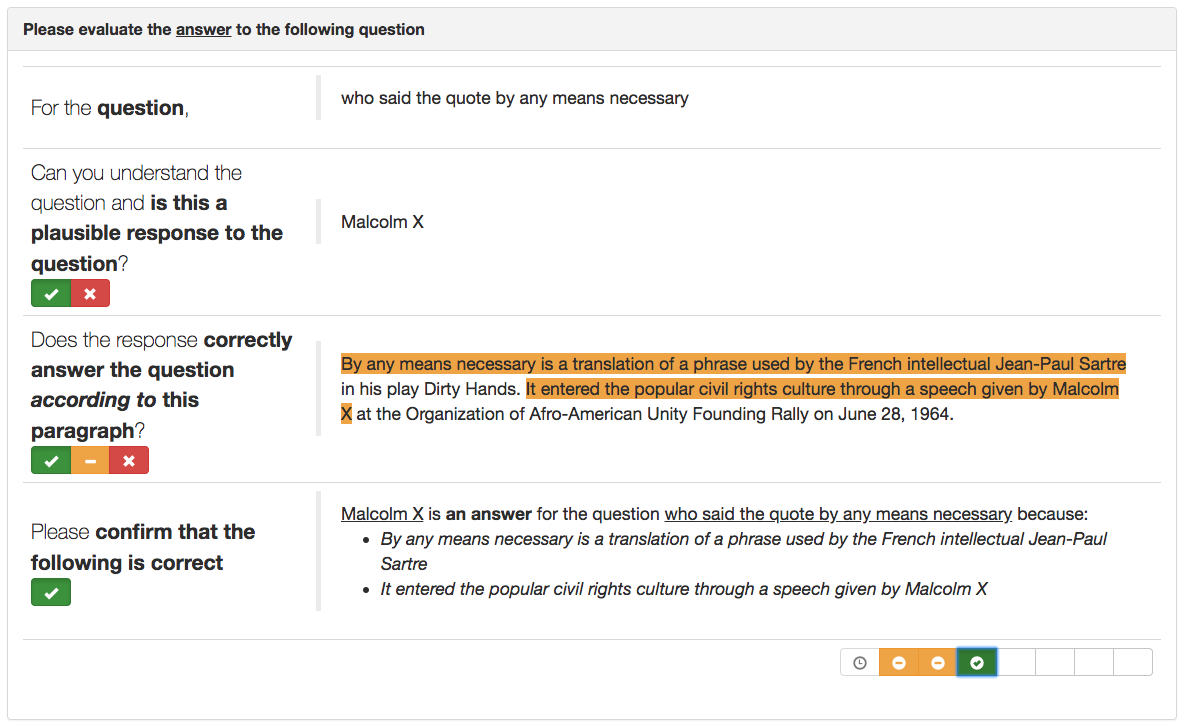
Each annotator was shown a question from the MS MARCO dataset and an answer that was generated by a system or provided as a reference answer from the dataset. The annotators were then asked to (a) rate if the question made sense and the answer was plausibly correct and (b) asked to identify which paragraphs provided in the dataset justified the answer (Figure 8(a)).
Interface design choices.
We found that some of the questions in the MS MARCO dataset were extremely ambiguous (e.g. “metatarsal what causes”) and some system responses were implausible (e.g “monogenic bone diseases”, for the question “what genes cause osteoporosis”). In these cases, annotators expressed confusion if they were forced to judge if the response was correct or incorrect. We resolved this confusion by first asking annotators if the question made sense and if system response was even plausible.
In early pilots, we found that annotators often rated a paragraph that correctly answered the question but was unrelated to the system response to be “correct”. We were able to resolve this problem by asking annotators to double-check their work (see the last question in Figure 8(a) for an example).
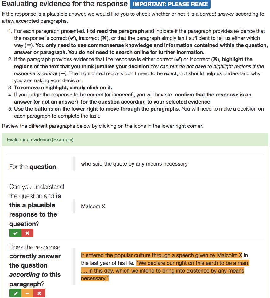
Once again, we forced annotators to complete an interactive tutorial containing eight questions each before beginning the task (Figure 8(b)). The tutorial also took about 5–6 minutes to complete and annotators were paid a one-time bonus of $0.75 on completion.
Quality control measures.
We found that requiring annotators to provide justification spans significantly spam. Additionally, we rejected annotators who took too little time to complete the task or had very low agreement rates on the answer correctness.
Appendix B Proofs
In this section, we provide proofs for the theorems stated in the main paper.
B.1 Main Theorem
In this section, we prove the main theorem (Theorem 3.1) in the paper about the minimax optimal variance for an unbiased estimator. Theorem 3.1 will follow from the two following lemmas (Lemmas B.1 and B.2). First, we show in Lemma B.1 that for all distributions with fixed , and , the variance of is constant and equal to: . Then we give an explicit distribution, a Gaussian distribution, where any estimator yields at least this variance using the theory of sufficient statistics. Together, these show that the max variance of any estimator is at least the max variance of .
As a reminder, the estimator is
| (8) |
where .
Lemma B.1.
The variance of is always
| (9) |
Proof.
By the law of total variance, with respect to the draws of ,
| (10) |
We will evaluate each of the two terms on the right hand side.
For the first term,
| (11) |
Because the human responses are uncorrelated,
| (12) | ||||
| (13) | ||||
| (14) |
For the second term,
| (15) |
Because the are sampled independently,
| (16) | ||||
| (17) |
Note that , , and (since it is normalized). Thus,
| (18) | ||||
| (19) |
Since the correlation ,
| (20) | ||||
| (21) |
Putting these two terms together, we find that,
| (22) | ||||
| (23) |
∎
For the next lemma, we show that the worst-case variance for any estimator is at least that of . For this, we will define a simple Gaussian distribution and use the theory of sufficient statistics. We explicitly define a distribution over , , and . In particular, we assume these are all Gaussian distributions with respective means, , and variances, . Additionally, we assume that and have covariance but is independent.
Lemma B.2.
is the minimal variance unbiased estimate (MVUE) for the Gaussian distribution above.
Proof.
The proof is straightforward: we first show that is a sufficient statistic using the Fisher-Neyman factorization theorem, and then we apply the Lehman-Scheffe theorem.
For ease of notation, define and . For the purposes of statistics, only is a parameter; the other “parameters” are known constants. Note that the pdf of the observed variables and is,
| (24) |
| (25) |
Thus, with the Fisher-Neyman factorization theorem, it suffices to show that the exponetiated term decomposes as a sum of a function that only depends on the data and a function that only depends on and .
| (26) |
Letting be the inverse determinant (which is constant),
| (27) | ||||
| (28) | ||||
| (29) | ||||
| (30) | ||||
| (31) |
Thus, we see the decomposition into the function of only the data on the right and only and on the left. Thus, is a sufficient statistic.
Further, is an unbiased estimate of since and .
Further, since is normally distributed with mean dependent on , it is complete.
Thus, by the Lehmann-Scheffe theorem, is the minimal variance unbiased estimate (MVUE).
∎
Theorem 3.1.
Among all unbiased estimators that are functions of and , and for all distributions with a given , , and ,
| (32) |
and no other estimator has a lower worst-case variance.
Proof.
From Lemma B.1 we have that the max variance of over all distributions with fixed variances, is exactly,
| (33) |
Further, from Lemma B.2, we know that is the MVUE for a particular class of distributions, thus, any estimator has a larger max variance over all distributions.
Combining these two facts, we get that the minimax variance is the variance of . ∎
B.2 Added Bias
Proof.
The bias is
| (34) | ||||
| (35) |
Since ,
| (36) | ||||
| (37) | ||||
| (38) | ||||
| (39) |
Because is independent and has mean ,
| (40) |
Because is mean zero and the are drawn independently,
| (41) | ||||
| (42) | ||||
| (43) | ||||
| (44) | ||||
| (45) |
∎