A Multigrid Algorithm with Non-Standard Smoother for Two Selective Models in Variational Segmentation

Abstract

Automatic segmentation of an image to identify all meaningful parts is one of the most challenging as well as useful tasks in a number of application areas. This is widely studied. Selective segmentation, less studied, aims to use limited user specified information to extract one or more interesting objects (instead of all objects). Constructing a fast solver remains a challenge for both classes of model. However our primary concern is on selective segmentation.

In this work, we develop an effective multigrid algorithm, based on a new non-standard smoother to deal with non-smooth coefficients, to solve the underlying partial differential equations (PDEs) of a class of variational segmentation models in the level set formulation. For such models, non-smoothness (or jumps) is typical as segmentation is only possible if edges (jumps) are present. In comparison with previous multigrid methods which were shown to produce an acceptable mean smoothing rate for related models, the new algorithm can ensure a small and global smoothing rate that is a sufficient condition for convergence. Our rate analysis is by Local Fourier Analysis and, with it, we design the corresponding iterative solver, improving on an ineffective line smoother. Numerical tests show that the new algorithm outperforms multigrid methods based on competing smoothers.

Keywords. Partial differential equations, multigrid, fast solvers, Local Fourier Analysis, image segmentation, jump coefficients.

1.   Introduction

Segmentation of an image into its individual objects is one incredibly important application of image processing techniques. Not only are accurate segmentation results required, but also it is required that the segmentation method is fast. Many imaging applications demand increasingly higher resolution e.g. an image of size 25000 $\times$ 25000 (or practically $10^{8}$ unknowns) can be common in oncology imaging. Here we address the problem of slow solutions by developing a fast multigrid method for PDEs arising from segmentation models.

Segmentation can take two forms; firstly global segmentation is the isolation of all objects in an image from the background and secondly, selective segmentation is the isolation of a subset of the objects in an image from the background. Selective segmentation is very useful in, for example, medical imaging for the segmentation of single organs.

Approaches to image segmentation broadly fall into two classes; region-based and edge-based. Some region-based approaches are region growing [1], watershed algorithms [37], Mumford-Shah [26] and Chan-Vese [15]. The final two of these are PDE-based variational approaches to the problem of segmentation. There are also models which mix the two classes to use the benefits of the region-based and edge-based approaches and will incorporate features of each. Edge-based methods aim to encourage an evolving contour towards the edges in an image and normally require an edge detector function [12]. The first edge-based variational approach was devised by Kass et al. [21] with the famous snakes model, this was further developed by Casselles et al. [12] who introduced the Geodesic Active Contour (GAC) model. Region-based global segmentation models include the well known works of Mumford-Shah [26] and Chan-Vese [15]. Importantly they are non-convex and hence a minimiser of these models may only be a local, not the global, minimum. Further work by Chan et al. [14] gave rise to a method to find the global minimiser for the Chan-Vese model under certain conditions.

Selective segmentation of objects in an image, given a set of points near the object or objects to be segmented, builds in such user input to a model using a set $\mathcal{S}=\{(x_{i},y_{i})\in\Omega,1\leq i\leq k\}$ where $\Omega\subset\mathbb{R}^{2}$ is the image domain [19, 5, 6]. Nguyen et al. [28] considered marker sets $\mathcal{S}$ and $\mathcal{A}$ which consist of points inside and outside, respectively, the object or objects to be segmented. Gout et al. [19] combined the GAC approach with the geometrical constraint that the contour pass through the points of $\mathcal{S}$. This was enforced with a distance function which is zero at $\mathcal{S}$ and non-zero elsewhere. Badshah and Chen [5] then combined the Gout et al. model with [15] to incorporate a constraint on the intensity in the selected region, thereby encouraging the contour to segment homogenous regions. Rada and Chen [30] introduced a selective segmentation method based on two-level sets which was shown to be more robust than the Badshah-Chen model. We also refer to [6, 22] for selective segmentation models which include different fitting constraints, using coefficient of variation and the centroid of $\mathcal{S}$ respectively.

None of these models have a restriction on the size of the object or objects to be detected and depending on the initialisation these methods have the potential to detect more or fewer objects than the user desired. To address this and to improve on [30], Rada and Chen [31] introduced a model (we refer to it as the Rada-Chen model from now on) combining the Badshah-Chen [5] model with a constraint on the area of the objects to be segmented. The reference area used to constrain the area within the contour is that of the polygon formed by the markers in $\mathcal{S}$. Spencer and Chen [33] recently introduced a model with the distance fitting penalty as a standalone term in the energy functional, unbounding it from the edge detector term of the Gout et al. model. All of the above selective segmentation models discussed are non-convex and hence the final result depends on the initialisation. Spencer and Chen [33], in the same paper, reformulated the model they introduced to a convex form using a penalty term as in [14]. We have considered the convex Spencer-Chen model but found that the numerical implementation is unfortunately sensitive to the main parameters and is unstable if they aren’t chosen correctly within a small range; hence we focus on the non-convex model they introduce for which reliable results have been found (we refer to this as the Spencer-Chen model from now on). A convex version of the Rada-Chen model cannot be formulated [33]. In this paper we only consider 2D images, however for completion we remark that 3D segmentation models do exist [23, 39].

Solving the PDE models, in the context of large scale images, quickly remains a challenge. The variational approach to image segmentation involves the minimisation of an energy functional such as that in [31]. This will typically involve solving a system of equations from a discretised PDE using an iterative method. In particular, discretisations of models such as [5, 6, 15, 31, 33] are non-linear and so require non-linear iterative methods to solve. The number of equations in the system is equal to the number of pixels in the image, which can be very large, and for each equation in the system the number of steps of an iterative method required can also be very large (to reach convergence). Due to improvements in technology and imaging, we now can produce larger and larger images, however this has the direct consequence that analysis of such images has become much more computationally intensive. We remark that if we directly discretise the variational models first (without using PDEs), Chan-Vese type models can be reformulated into minimisation based on graph cuts and then fast algorithms have been proposed [7, 25].

The multigrid approach for solving PDEs in imaging has been tried before and previous work by Badshah and Chen [3, 4] introduced a 2D Chan-Vese multigrid algorithm for two-phase and multi-phase images, additionally Zhang et al. [39] implemented a multigrid algorithm for the 3D Chan-Vese model. The fundamental idea behind multigrid is that if we perform most of the computations on a reduced resolution image then the computational expense is lower. We then transfer our solution from the low resolution grid to the high resolution grid through interpolation and smooth out any errors which have been introduced by the interpolation using a few steps of a smoothing algorithm, e.g. Gauss-Seidel. The multigrid method is an optimal solver when it converges [24, 34]. This requires that the smoothing scheme, which corrects the errors when transferring between the higher and lower resolution images and vice-versa, is effective, i.e. reduces the error magnitude of high-frequency components quickly.

In the large literature of multigrid methods, the convergence problem associated with non-smooth or jumping coefficients was often highlighted [2, 11] and developing working algorithms which converge is a key problem. Much attention was given to designing better coarsening strategies and improved interpolation operators [38, 40] while keeping the simple smoothers; such as the damped Jacobi, Gauss-Seidel or line smoothers. In practice, one can quickly exhaust the list of standard smoothers and yet cannot find a suitable one unless compromising in optimality by increasing the number of iterations. In contrast, our approach here is to seek a non-standard and more effective smoother with an acceptable smoothing rate. Our work is motivated by Napov and Notay [27] who established the explicit relationship of a smoothing rate to the underlying multigrid convergence rate for linear models; in particular the former also serves as the lower bound for the latter.

The contributions of this paper can be summarised as follows: (1) We review six smoothers for the Rada-Chen and Spencer-Chen selective segmentation models and perform Local Fourier Analysis (LFA) to assess their performance and quantitatively determine their effectiveness (or lack of). (2) We propose an effective non-linear multigrid method to solve the Rada-Chen model [31] and the Spencer-Chen model [33], based on a new smoothers that add non-standard smoothing steps locally at coefficient jumps. We recommend in particular one of our new hybrid smoothers which achieves a better smoothing rate than the other smoothers studied and thus gives rise to a multigrid framework which converges to the energy minimiser faster than when standard smoothers are used.

The remainder of this paper is structured as follows; in §2 we review some global and selective segmentation models building to the Rada-Chen and Spencer-Chen models. In §3 we describe the Full Approximation Scheme multigrid framework, give details of six smoothers that we consider and compare the smoothing rates. We find that none of these standard smoothers can produce a small enough smoothing rate to yield an effective multigrid method and so in §4 we then introduce two new hybrid smoothers based on new iterative schemes to improve the smoothing rates at those pixels where the six smoothers perform badly. In §5 we test our algorithms with some numerical results, recommend the best algorithm using one of our proposed smoothers and analyse the complexity of the recommended multigrid algorithm. Finally in §6 we provide some concluding remarks.

2.   Review of segmentation models

Our methods will apply to both global segmentation models and selective segmentation models. It is necessary to briefly describe both types. Denote a given image in domain $\Omega\subset\mathbb{R}^{2}$ by $z(x,y)$.

2.1.   Global segmentation models

The model of Mumford and Shah [26] is one of the most famous and important variational models in image segmentation. We will review its two-dimensional piecewise constant variant, commonly known as the Chan-Vese (CV) model [15], which takes the form

$$\min_{\Gamma,c_{1},c_{2}}F_{CV}(\Gamma,c_{1},c_{2})=\mu\cdot length(\Gamma)+\lambda_{1}\int_{\Omega_{1}}|z(x,y)-c_{1}|^{2}d\Omega+\lambda_{2}\int_{\Omega_{2}}|z(x,y)-c_{2}|^{2}d\Omega$$ (1)

where the foreground $\Omega_{1}$ is the subdomain to be segmented, the background is $\Omega_{2}=\Omega\backslash\Omega_{1}$ and $\mu,\lambda_{1},\lambda_{2}$ are fixed non-negative parameters. The values $c_{1}$ and $c_{2}$ are the average intensities of $z(x,y)$ inside $\Omega_{1}$ and $\Omega_{2}$ respectively. Using the ideas of Osher and Sethian [29], a level set function

$$\phi(x,y)=\begin{cases}>0,&(x,y)\in\Omega_{1},\\ 0,&(x,y)\in\Gamma,\\ <0,&otherwise,\\ \end{cases}$$

is used by [15] to track the object boundary $\Gamma$, where we now define it as the zero level set of $\phi$, i.e. $\Gamma=\{(x,y)\in\Omega\,|\,\phi(x,y)=0\}$. We reformulate (1) as

$$\begin{split}\min_{\phi,c_{1},c_{2}}F_{CV}(\phi,c_{1},c_{2})=&\mu\int_{\Omega}|\nabla H_{\varepsilon}(\phi)|d\Omega+\lambda_{1}\int_{\Omega}(z(x,y)-c_{1})^{2}H_{\varepsilon}(\phi)d\Omega\\ &\ \hskip 76.82234pt+\lambda_{2}\int_{\Omega}(z(x,y)-c_{2})^{2}(1-H_{\varepsilon}(\phi))d\Omega,\\ \end{split}$$ (2)

with $H_{\varepsilon}(\phi)$ a smoothed Heaviside function such as [15]

$$H_{\varepsilon}(\phi)=\frac{1}{2}+\frac{1}{\pi}\arctan\bigg{(}\frac{\phi}{\varepsilon}\bigg{)}$$

where we use $\varepsilon=1$ in our experiments. We solve this minimisation problem in two stages, first with $\phi$ fixed we minimise with respect to $c_{1}$ and $c_{2}$, yielding

$$c_{1}=\frac{\int_{\Omega}H_{\varepsilon}(\phi)\cdot z(x,y)\,d\Omega}{\int_{\Omega}H_{\varepsilon}(\phi)\,d\Omega},\hskip 36.135ptc_{2}=\frac{\int_{\Omega}(1-H_{\varepsilon}(\phi))\cdot z(x,y)\,d\Omega}{\int_{\Omega}(1-H_{\varepsilon}(\phi))\,d\Omega},$$ (3)

and secondly, with $c_{1}$ and $c_{2}$ fixed we minimise (2) with respect to $\phi$. This requires the determination of the associated Euler-Lagrange form [15] and then solving the resulting PDE. A drawback of the Chan-Vese functional (2) is that it is non-convex. Therefore a minimiser of this functional may only be a local minimum and not the global minimum. Hence the final segmentation result is dependent on the initial contour. Chan et al. [14] reformulated (2) to obtain an equivalent convex model and hence we can always obtain the global minimum for this model.

2.2.   Selective segmentation models

Selective segmentation models make use of user input, being a marker set of points near the object or objects to be segmented. Let $\mathcal{S}=\{(x_{i},y_{i})\in\Omega,1\leq i\leq k\}$ be such a marker set. The contour is encouraged to pass through or near the points of $\mathcal{S}$ by a distance function such as [23]

$$d(x,y)=\prod^{k}_{i=1}\Big{(}1-e^{-\frac{(x_{i}-x)^{2}}{2\sigma^{2}}}e^{-\frac{(y_{i}-y)^{2}}{2\sigma^{2}}}\Big{)},\ \ \forall(x,y)\in\Omega,(x_{i},y_{i})\in\mathcal{S},$$

where $\sigma$ is a fixed non-negative tuning parameter. See, for example, [19, 33] for other distance functions. The distance function is zero at the points of $\mathcal{S}$ and non-zero elsewhere, taking a maximum value of one. Gout et al. [23] were the first to introduce a model incorporating a distance function into the Geodesic Active Contour model of Caselles et al. [12], however this model struggles when boundaries between objects and their background are fuzzy or blurred. To address this, Badshah and Chen [5] introduced a new model which includes the intensity fitting terms from the CV model (1). However this model has poor robustness [30] if iterating for too many steps the final segmentation can include more or fewer objects than intended. To improve on this, Rada and Chen [31] introduced a model which incorporates an area fitting term into the Badshah-Chen (BC) model and is far more robust.

The Rada-Chen model [31]. This is the first model we focus on in this paper, defined by

$$\begin{split}F_{RC}(\phi,c_{1},c_{2})=&\mu\int_{\Omega}d(x,y)g(|\nabla z(x,y)|^{2})|\nabla H_{\varepsilon}(\phi)|dxdy\\ &+\lambda_{1}\int_{\Omega}(z(x,y)-c_{1})^{2}H_{\varepsilon}(\phi)dxdy+\lambda_{2}\int_{\Omega}(z(x,y)-c_{2})^{2}(1-H_{\varepsilon}(\phi))dxdy\\ &+\nu\bigg{[}\left(\int_{\Omega}H_{\varepsilon}(\phi)dxdy-A_{1}\right)^{2}+\left(\int_{\Omega}(1-H_{\varepsilon}(\phi))dxdy-A_{2}\right)^{2}\bigg{]},\end{split}$$ (4)

where $\mu,\lambda_{1},\lambda_{2},\nu$ are fixed non-negative parameters. The edge detector function $g(|\nabla z(x,y)|^{2})$ is given by $g(s)=1/(1+\beta s)$ for tuning parameter $\beta$ which takes value $0$ at edges and is $1$ away from them. $A_{1}$ is the area of the polygon formed from the points of $\mathcal{S}$ and $A_{2}=|\Omega|-A_{1}$. The final term of this functional therefore puts a penalty on the area inside a contour being very different to $A_{1}$. The first variation of (4) with respect to $\phi$ gives the Euler-Lagrange form [31]

$$\begin{gathered}\delta_{\varepsilon}(\phi)\bigg{\{}\mu\nabla\cdot\left(\frac{d(x,y)\cdot g(|\nabla z(x,y)|^{2})\nabla\phi}{|\nabla\phi|}\right)-\Big{[}\lambda_{1}(z(x,y)-c_{1})^{2}-\lambda_{2}(z(x,y)-c_{2})^{2}\Big{]}\bigg{.}\\ \bigg{.}-\nu\bigg{[}(\int_{\Omega}H_{\varepsilon}(\phi)dxdy-A_{1})-(\int_{\Omega}(1-H_{\varepsilon}(\phi))-A_{2})\bigg{]}\bigg{\}}=0,\\ \end{gathered}$$ (5)

in $\Omega$ with the condition that $\frac{\partial\phi}{\partial\bm{n}}=0$ on $\partial\Omega$, $\bm{n}$ the outward normal vector and $\delta_{\varepsilon}(\phi)=\frac{dH_{\varepsilon}(\phi)}{d\phi}$.

Discretisation of the Rada-Chen model. We denote by $\phi_{i,j}=\phi(x_{i},y_{j})$ the approximation of $\phi$ at $(i,j)$ for $1\leq i\leq n$ and $1\leq j\leq m$. We let $h_{x}$ and $h_{y}$ be the grid spacings in the $x$ and $y$ directions respectively. Using finite differences, and noting $A_{2}=1-A_{1}$, we obtain the scheme

$$\begin{gathered}\ A_{i,j}\phi_{i+1,j}+B_{i,j}\phi_{i-1,j}+C_{i,j}\phi_{i,j+1}+D_{i,j}\phi_{i,j-1}-S_{i,j}\phi_{i,j}\\ \qquad-\delta_{\varepsilon}(\phi_{i,j})\bigg{\{}\bigg{[}\lambda_{1}(z_{i,j}-c_{1})^{2}-\lambda_{2}(z_{i,j}-c_{2})^{2}\bigg{]}-2\nu\bigg{[}h_{x}h_{y}\sum_{k,l}H_{\varepsilon}(\phi_{k,l})-A_{1}\bigg{]}\bigg{\}}=0,\\ \end{gathered}$$ (6)

where  $\displaystyle G_{i,j}=\frac{d_{i,j}\cdot g(|\nabla z_{i,j}|)}{|\nabla\phi_{i,j}|},\quad A_{i,j}=\frac{\mu\delta_{\varepsilon}(\phi_{i,j})}{h_{x}^{2}}G_{i+\frac{1}{2},j},\quad B_{i,j}=\frac{\mu\delta_{\varepsilon}(\phi_{i,j})}{h_{x}^{2}}G_{i-\frac{1}{2},j},$

$$\begin{gathered}C_{i,j}=\frac{\mu\delta_{\varepsilon}(\phi_{i,j})}{h_{y}^{2}}G_{i,j+\frac{1}{2}},\quad D_{i,j}=\frac{\mu\delta_{\varepsilon}(\phi_{i,j})}{h_{y}^{2}}G_{i,j-\frac{1}{2}},\quad S_{i,j}=A_{i,j}+B_{i,j}+C_{i,j}+D_{i,j},\end{gathered}$$ (7)

The Spencer-Chen model [33]. The second model we focus on in this paper is defined by

$$\begin{split}F_{SC}(\phi,c_{1},c_{2})=&\mu\int_{\Omega}g(|\nabla z(x,y)|^{2})|\nabla H_{\varepsilon}(\phi)|dxdy+\lambda_{1}\int_{\Omega}(z(x,y)-c_{1})^{2}H_{\varepsilon}(\phi)dxdy\\ &+\lambda_{2}\int_{\Omega}(z(x,y)-c_{2})^{2}(1-H_{\varepsilon}(\phi))dxdy+\theta\int_{\Omega}d(x,y)H_{\varepsilon}(\phi)dxdy,\end{split}$$ (8)

where $\mu,\lambda_{1},\lambda_{2}$ and $\theta$ are fixed non-negative parameters. Note that this model differs from the Rada-Chen model (4) as the distance function has been separated from the edge detector term and is now a standalone penalty term. This model has Euler-Lagrange form

$$\begin{split}\delta_{\varepsilon}(\phi)\left\{\mu\nabla\cdot\left(\frac{g(|\nabla z(x,y)|^{2})\nabla\phi}{|\nabla\phi|}\right)-\left[\lambda_{1}(z(x,y)-c_{1})^{2}-\lambda_{2}(z(x,y)-c_{2})^{2}\right]-\theta d(x,y)\right\}=0,\\ \end{split}$$ (9)

in $\Omega$ with the condition that $\frac{\partial\phi}{\partial\bm{n}}=0$ on $\partial\Omega$, again with $\bm{n}$ the outward normal vector. We discretise this similarly to the Rada-Chen model previously.

3.   Non-linear multigrid Algorithm 1

Segmentation using a non-linear multigrid algorithm has been explored by Badshah and Chen [3, 4] for the Chan-Vese model [15] and the Vese-Chan model [36] which are global segmentation models. A multigrid method has not yet been applied to selective segmentation and this is the main task of this paper, to apply the multigrid method to the Rada-Chen (4) and Spencer-Chen (8) selective segmentation models. However as we will see shortly, the task is challenging as standard methods do not work. For brevity we will restrict consideration just to the Rada-Chen model as the derivations for the Spencer-Chen model are similar.

3.1.   The Full Approximation Scheme

To solve the Rada-Chen model we must solve the non-linear system (6) and so we will use the non-linear Full Approximation Scheme [13, 16, 20, 34] algorithm due to Brandt [9]. Denote a discretised system by

$$N^{h}\phi^{h}=f^{h},$$ (10)

where $h$ indicates that these are the functions on the $n\times m$ cell-centred grid $\Omega^{h}$ and $N^{h}$ is the discretised non-linear operator (which contains the boundary conditions). Similarly define the grids $\Omega^{2h}$ as the $\frac{n}{2}\times\frac{m}{2}$ cell-centred grid resulting from the standard coarsening [34] of $\Omega^{h}$, we indicate functions on $\Omega^{2h}$ by $f^{2h},N^{2h}$ and $\phi^{2h}$. Let $\Phi^{h}$ be an approximation to $\phi^{h}$ such that the error $e^{h}=\phi^{h}-\Phi^{h}$ is smooth. Define the residual as $r^{h}=f^{h}-N^{h}\Phi^{h}$. Therefore using (10) we have the residual equation

$$N^{h}(\Phi^{h}+e^{h})-N^{h}\Phi^{h}=r^{h}.$$

If the error $e^{h}$ is smooth then this can be well approximated on $\Omega^{2h}$; the assumption can be a big issue for non-linear problems. With an approximation of $e^{h}$ on $\Omega^{2h}$ we can solve the residual equation on $\Omega^{2h}$, which is significantly less computationally expensive than solving on $\Omega^{h}$, and then transfer this error to $\Omega^{h}$ and use it to correct the approximation $\Phi^{h}$. This method, using the two grids $\Omega^{2h}$ and $\Omega^{h}$, is called a two-grid cycle and it can be nested such that we can consider solving on $\Omega^{4h},\Omega^{8h},\ldots$ and transferring the errors up through the levels to $\Omega^{h}$ and smoothing on each level. This is the multigrid method. We transfer from $\Omega^{h}$ to $\Omega^{2h}$ by restriction and from $\Omega^{2h}$ to $\Omega^{h}$ by interpolation.

Restriction. We use the full-weighting operator $I^{2h}_{h}\Phi^{h}=\Phi^{2h}$ [34]

$$\begin{gathered}\begin{aligned} \phi^{2h}_{i,j}=\frac{1}{16}\Big{[}\phi^{h}_{2i-1,2j-1}+2\phi^{h}_{2i-1,2j}&+\phi^{h}_{2i-1,2j+1}+2\phi^{h}_{2i,2j-1}+4\phi^{h}_{2i,2j}\\ &+2\phi^{h}_{2i,2j+1}+\phi^{h}_{2i+1,2j-1}+2\phi^{h}_{2i+1,2j}+\phi^{h}_{2i+1,2j+1}\Big{]},\\ \end{aligned}\end{gathered}$$

and at boundary pixels $\phi^{2h}_{i,m}=\frac{1}{2}\left[\phi^{h}_{2i,m-1}+\phi^{h}_{2i,m}\right]$ and $\phi^{2h}_{n,j}=\frac{1}{2}\left[\phi^{h}_{n-1,2j}+\phi^{h}_{n,2j}\right].$

Interpolation. We use a bilinear interpolation operator $I^{h}_{2h}\Phi^{2h}=\Phi^{h}$ [34]

$$\phi^{h}_{2i,2j}=\phi^{2h}_{i,j},\hskip 36.135pt\phi^{h}_{2i+1,2j}=\frac{1}{2}\left[\phi^{2h}_{i,j}+\phi^{2h}_{i+1,j}\right],\hskip 36.135pt\phi^{h}_{2i,2j+1}=\frac{1}{2}\left[\phi^{2h}_{i,j}+\phi^{2h}_{i,j+1}\right],$$

$$\phi^{h}_{2i+1,2j+1}=\frac{1}{4}\left[\phi^{2h}_{i,j}+\phi^{2h}_{i+1,j}+\phi^{2h}_{i,j+1}+\phi^{2h}_{i+1,j+1}\right].$$

We now move to the most important element of the multigrid method – the smoother. As previously mentioned, we need $e^{h}$ to be smooth to ensure that $\Phi^{h}$ is a good approximation to $\phi^{h}$. In practice, we smooth $e^{h}$ by using an iterative method such as Gauss-Seidel [3, 4] and the success or failure of a multigrid method hinges on the effectiveness of it at smoothing the errors.

3.2.   Smoothers for the Rada-Chen [31] model

Gauss-Seidel and Newton iterative methods have been shown to be effective smoothers for PDE problems with smooth coefficients [34, 38]. In this subsection we look at three distinct smoothing iterative techniques; lexicographic Gauss-Seidel, line Gauss-Seidel and Newton smoothers. For each of these smoothers we consider two different approaches for fixing the coefficients in the scheme - globally or locally. Hence overall we consider six smoothers for [31]; the same smoothers are adaptable for [33] in a simple way.

Smoothers 1-2 (GSLEX I - II). Lexicographic Gauss-Seidel smoothers are widely used in multigrid methods [3, 34]. We update $\phi_{i,j}$ one at a time and work across and down through the grid of pixels in an image. Lexicographic Gauss-Seidel smoothers for the Rada-Chen model [31]. We can rearrange (6) as

$$\phi_{i,j}=\big{(}A_{i,j}\phi_{i+1,j}+B_{i,j}\phi_{i-1,j}+C_{i,j}\phi_{i,j+1}+D_{i,j}\phi_{i,j-1}-f_{i,j}\big{)}\ \big{/}\ S_{i,j},$$ (11)

where $f_{i,j}=\delta_{\varepsilon}(\phi_{i,j})\Big{\{}\big{[}\lambda_{1}(z_{i,j}-c_{1})^{2}-\lambda_{2}(z_{i,j}-c_{2})^{2}\big{]}+2\nu\big{[}+h_{x}h_{y}\sum_{k,l}H_{\varepsilon}(\phi_{k,l})-A_{1}\big{]}\Big{\}},$ to obtain a fixed point scheme for the Rada-Chen model. There are two approaches for implementing this smoother; either update the coefficients globally at the start of each outer iteration or update them locally, immediately after solving for each pixel value. We denote the global smoother by GSLEX-I and the local smoother by GSLEX-II. In the algorithm for both smoothers, we cycle through each pixel $(i,j)$ in turn solving (11) and updating the value of $\phi(i,j)$, only with GSLEX-II do we update the coefficients immediately and they are used in the update of $\phi(i,j)$ on the next iteration.

Smoothers 3-4 (GSLINE I - II). Line smoothers are often used for harder problems (e.g. anisotropic coefficients). Here we perform the Gauss-Seidel updates one column at a time but the approach can be easily reformulated for a row by row update.

Gauss-Seidel line smoothers for the Rada-Chen model [31]. If we rearrange (6) to have all the $\phi_{\cdot,j}$ terms on the left hand side we obtain

$$\begin{gathered}A_{i,j}\phi_{i+1,j}+B_{i,j}\phi_{i-1,j}-S_{i,j}\phi_{i,j}=F_{i,j}=-C_{i,j}\,\phi_{i,j+1}-D_{i,j}\phi_{i,j-1}+f_{i,j},\\ \end{gathered}$$ (12)

where we can reformulate (12) as the following tridiagonal system

This system is diagonally dominant (by definition (7)) and if $C_{i,j}+D_{i,j}\neq 0$ then the system is strictly diagonally dominant. We can choose parameters for the edge detector and distance function which ensure this is always true. Therefore this will ensure that the Gauss-Seidel line smoother will converge to a solution [18]. As before, we obtain two smoothers; the global smoother GSLINE-I and the local smoother GSLINE-II.

Smoothers 5-6 (NEWT I - II). Our last set of smoothers rely on the Newton fixed point iteration schemes.

Newton smoothers for the Rada-Chen model [31]. We can rewrite (6) in a non-linear form for $\phi_{i,j}$

$$S_{i,j}\phi_{i,j}^{(k)}-P_{i,j}+Q_{i,j}(\phi_{i,j}^{(k)})=0.$$

where $P_{i,j}=A_{i,j}\phi_{i+1,j}+B_{i,j}\phi_{i-1,j}+C_{i,j}\phi_{i,j+1}+D_{i,j}\phi_{i,j-1}-\delta_{\varepsilon}(\phi_{i,j})\left[\lambda_{1}(z_{i,j}-c_{1})^{2}-\lambda_{2}(z_{i,j}-c_{2})^{2}\right]$ and $Q_{i,j}=2\nu\delta_{\varepsilon}(\phi_{i,j})\left[h_{x}h_{y}\sum_{k,l}H_{\varepsilon}(\phi_{k,l})-A_{1}\right]$. The Newton scheme to compute $\phi_{i,j}^{(k+1)}$ is

$$\phi_{i,j}^{(k+1)}=\phi_{i,j}^{(k)}-\big{(}S_{i,j}\phi_{i,j}^{(k)}-P_{i,j}+Q_{i,j}(\phi_{i,j}^{(k)})\big{)}\ \big{/}\ \big{(}S_{i,j}+Q_{i,j}^{\prime}(\phi_{i,j}^{(k)})\big{)}$$ (14)

where $Q_{i,j}^{\prime}(\phi_{i,j}^{(k)})=2\nu\delta_{\varepsilon}(\phi_{i,j})^{2}h_{x}h_{y}+2\nu\delta_{\varepsilon}^{\prime}(\phi_{i,j}))\Big{[}h_{x}h_{y}\sum_{k,l}H_{\varepsilon}(\phi_{k,l})-A_{1}\Big{]}$. We again have a global smoother, NEWT-I, and a local smoother, NEWT-II.

3.3.   Algorithm 1

In §3.1 we briefly discussed the FAS across two grids, $\Omega^{h}$ (the fine grid) and $\Omega^{2h}$ (the coarse grid). The two-grid cycles can be nested so we can perform the majority of the computations on coarser grids than $\Omega^{2h}$, such as $\Omega^{4h},\Omega^{8h},etc$ and recursive use of $V$-cycles gives rise to multigrid schemes [34]. The general non-linear multigrid Full Approximation Scheme algorithm is given by Algorithm 1.

  Pre-smoothing: Perform $\nu_{1}$ iterations of the smoother: $\phi^{h}\leftarrow Smoother(\phi^{h},f^{h},\nu_{1}).$

  Coarse grid correction:    Compute the residual: $r^{h}=f^{h}-N^{h}\overline{\phi}^{h}.$

  Transfer the residual to $\Omega^{2h}$ by restriction: $r^{2h}=I^{2h}_{h}r^{h}.$

  Compute: $\phi^{2h}=I^{2h}_{h}\phi^{h},\Phi^{2h}=\phi^{2h},\overline{f}^{2h}=N^{2h}\phi^{2h}+r^{2h}.$

  if $level=max\_level$ then

                                   Compute the exact solution $\phi^{2h}$ of $N^{2h}(\phi^{2h})=N^{2h}(\Phi^{2h})+r^{2h}$

                                   on $\Omega^{2h}$ using e.g. time-marching [15] or AOS [34].

  else

                                   Perform $\gamma$ cycles (steps) of

                                   $\phi^{2h}\leftarrow FASMG(\phi^{2h},N^{2h},f^{2h},\gamma,\nu_{1},\nu_{2},level+1,max\_level,Smoother)$.

  end if

  Interpolation:     Compute: $e^{2h}=\phi^{2h}-\Phi^{2h}.$

  Transfer the error to $\Omega^{h}$ by interpolation: $e^{h}=I_{2h}^{h}e^{2h}.$

  Correct the fine grid approximation: $\phi^{h}=\phi^{h}+e^{h}.$

  Post-smoothing: Perform $\nu_{2}$ iterations of the smoother: $\phi^{h}\leftarrow Smoother(\phi^{h},f^{h},\nu_{2}).$

Algorithm 1 FAS multigrid algorithm, $\phi^{h}\leftarrow FASMG(\phi^{h},N^{h},f^{h},\gamma,\nu_{1},\nu_{2},level,max\_level,Smoother)$

3.4.   Local Fourier Analysis of Algorithm 1 for the Rada-Chen Model

Local Fourier Analysis (LFA) is a useful tool for finding a quantitative measure for the effectiveness of a smoother [9, 16, 34]. It is designed to study linear problems with constant coefficients on an infinite grid. However, it is a standard and recommended [9, 11] tool to analyse non-linear operators. To overcome the limitations, we neglect the boundary conditions, extend the operator to an infinite grid and assume that we can linearise the operator locally (we do this by freezing the coefficients). LFA measures the largest amplification factor on high-frequency errors, for example if there is a smoothing rate of 0.8 this means that the high-frequency errors are damped by at least 20%. We initially must derive formulas for the approximation error at each pixel in our 5-point stencil.

Error forms. Using the definition of $f_{i,j}$, we can rewrite (6) as

$$A_{i,j}\phi_{i+1,j}+B_{i,j}\phi_{i-1,j}+C_{i,j}\phi_{i,j+1}+D_{i,j}\phi_{i,j-1}-S_{i,j}\phi_{i,j}=f_{i,j},$$ (15)

where we fix $A_{i,j},B_{i,j},C_{i,j}$ and $D_{i,j}$ based on a previous iteration. The GSLEX I-II and NEWT I-II schemes all work in a lexicographic manner, and so if we denote the previous iteration as the $k$-th we can rewrite (15) as

$$A_{i,j}\phi_{i+1,j}^{(k)}+B_{i,j}\phi_{i-1,j}^{(k+1)}+C_{i,j}\phi_{i,j+1}^{(k)}+D_{i,j}\phi_{i,j-1}^{(k+1)}-S_{i,j}\phi_{i,j}^{(k+1)}=f_{i,j},$$ (16)

and we obtain the error form by subtracting (16) from (15)

$$A_{i,j}e_{i+1,j}^{(k)}+B_{i,j}e_{i-1,j}^{(k+1)}+C_{i,j}e_{i,j+1}^{(k)}+D_{i,j}e_{i,j-1}^{(k+1)}-S_{i,j}e_{i,j}^{(k+1)}=0,$$ (17)

Using a similar argument, we obtain the following error form for the line smoothers GSLINE I-II

$$A_{i,j}e_{i+1,j}^{(k+1)}+B_{i,j}e_{i-1,j}^{(k+1)}+C_{i,j}e_{i,j+1}^{(k)}+D_{i,j}e_{i,j-1}^{(k+1)}-S_{i,j}e_{i,j}^{(k+1)}=0,$$ (18)

where $e_{i,j}^{(k)}=\phi_{i,j}-\phi_{i,j}^{(k)}$ and $e_{i,j}^{(k+1)}=\phi_{i,j}-\phi_{i,j}^{(k+1)}$.

Local Fourier Analysis. Define a general Fourier component by

$$F_{\theta_{1},\theta_{2}}(x_{i},y_{j})=\exp\left(2\pi{\bf i}\frac{\theta_{1}i}{n}\right)\cdot\exp\left(2\pi{\bf i}\frac{\theta_{2}j}{m}\right)=\exp\left({\bf i}\frac{\alpha_{1}x_{i}}{h_{x}}\right)\cdot\exp\left({\bf i}\frac{\alpha_{2}y_{j}}{h_{y}}\right),$$

where $\alpha_{1}=\frac{2\theta_{1}\pi}{n}$ and $\alpha_{2}=\frac{2\theta_{2}\pi}{m}$ and ${\bf i}$ is the imaginary unit. Note that $\alpha_{1},\alpha_{2}\in[-\pi,\pi]$. If we assume for simplicity that the image is square and hence $n=m$, we first expand

$$e^{(k+1)}_{i,j}=\sum^{n/2}_{\theta_{1},\theta_{2}=-n/2}\psi^{(k+1)}_{\theta_{1},\theta_{2}}F_{\theta_{1},\theta_{2}}(x_{i},y_{j}),\hskip 36.135pte^{(k)}_{i,j}=\sum^{n/2}_{\theta_{1},\theta_{2}=-n/2}\psi^{(k)}_{\theta_{1},\theta_{2}}F_{\theta_{1},\theta_{2}}(x_{i},y_{j}),$$

in Fourier components and define the smoothing rate $\hat{\mu}_{i,j}$ by [34, 16]

$$\hat{\mu}_{i,j}=\max_{\theta_{1},\theta_{2}}\mu(\theta_{1},\theta_{2})=\max_{\theta_{1},\theta_{2}}\left|\frac{\psi_{\theta_{1},\theta_{2}}^{(k+1)}}{\psi_{\theta_{1},\theta_{2}}^{(k)}}\right|,$$

in the high-frequency range where $(\alpha_{1},\alpha_{2})=(\frac{2\theta_{1}\pi}{n},\frac{2\theta_{2}\pi}{n})\in[-\pi,\pi)^{2}\backslash[-\frac{\pi}{2},\frac{\pi}{2})^{2}$. Since $\hat{\mu}_{i,j}$ is pixel dependent (non-linear problems), we may also call it the amplification factor associated with $(i,j)$.

Smoothing rates. For the GSLEX I-II, NEWT I-II smoothers, using (17) and (18), we obtain error amplification at pixel $(i,j)$

$$\hat{\mu}_{i,j}=\max_{\theta_{1},\theta_{2}}\mu(\theta_{1},\theta_{2})=\max_{\alpha_{1},\alpha_{2}}\left|\frac{A_{i,j}e^{{\bf i}\alpha_{1}}+C_{i,j}e^{{\bf i}\alpha_{2}}}{B_{i,j}e^{-{\bf i}\alpha_{1}}+D_{i,j}e^{-{\bf i}\alpha_{2}}-S_{i,j}}\right|,$$

and similarly for the GSLINE I-II smoothers we have

$$\hat{\mu}_{i,j}=\max_{\theta_{1},\theta_{2}}\mu(\theta_{1},\theta_{2})=\max_{\alpha_{1},\alpha_{2}}\left|\frac{C_{i,j}e^{{\bf i}\alpha_{2}}}{A_{i,j}e^{{\bf i}\alpha_{1}}+B_{i,j}e^{-{\bf i}\alpha_{1}}+D_{i,j}e^{-{\bf i}\alpha_{2}}-S_{i,j}}\right|.$$ (19)

Comparison of smoothing rates for all smoothers. We consider two different measures of the smoothing rates; the maximum and average over all pixels $(i,j)$. We define these in the obvious way as

$$\tilde{\mu}_{\text{max}}=\max_{i,j}\hat{\mu}_{i,j}=\max_{i,j}\max_{\theta_{1},\theta_{2}}\mu(\theta_{1},\theta_{2})\quad\mbox{and}\quad\tilde{\mu}_{\text{avg}}=\frac{\sum_{i,j}\hat{\mu}_{i,j}}{n^{2}}=\frac{\sum_{i,j}\max_{\theta_{1},\theta_{2}}\mu(\theta_{1},\theta_{2})}{n^{2}}.$$

Each of the smoothers was implemented in Algorithm 1 on the image in Figure 1(a) with a V-cycle ($\gamma=1$) and using a $1024\times 1024$ resolution image as the finest grid and a $32\times 32$ image as the coarsest grid and in Table 1 we give $\tilde{\mu}_{\max}$ and $\tilde{\mu}_{\text{avg}}$ for the Rada-Chen and Spencer-Chen models.

Smoother	Rada-Chen		Spencer-Chen
	$\tilde{\mu}_{\text{max}}$	$\tilde{\mu}_{\text{avg}}$	$\tilde{\mu}_{\text{max}}$	$\tilde{\mu}_{\text{avg}}$
GSLINE-I	0.9997	0.4800	0.9990	0.4586
GSLINE-II	0.9997	0.3782	1.0000*	0.4893
GSLEX-I	0.9978	0.5807	0.9927	0.5269
GSLEX-II	1.0000*	0.5244	0.9996	0.5512
NEWT-I	0.9985	0.5642	0.9595	0.4839
NEWT-II	0.9999	0.5749	0.9950	0.5133

Table 1: Smoothers and the associated maximum and average smoothing rates for the Rada-Chen and Spencer-Chen models. * due to rounding.

In the spirit of previous works [3], for any of these smoothers, one would quote $\tilde{\mu}_{\text{avg}}$, and although this appears to be an excellent rate in all cases, it is the rate $\tilde{\mu}_{\text{max}}$ that determines the multigrid convergence [27]. We therefore choose to focus on $\tilde{\mu}_{\text{max}}$. Table 1 shows us that $\tilde{\mu}_{\max}$ is better for the global smoothers compared to the local smoothers, this is in agreement with the results in [3]. However, the maximum smoothing rate of all of the smoothers is bad and so they cannot be implemented in a successful multigrid scheme. We look to improve the maximum smoothing rate of one of the better schemes to obtain a smoother which can be implemented successfully. In the next section we will see that the problem is due to discontinuous coefficients in the numerical schemes, and so we look to [2, 17] which recommend the use of line smoothers rather than a pixel-by-pixel update approach. We therefore choose the GSLINE-I smoother and review its performance for the Rada-Chen model in detail to see if we can improve the maximum smoothing rate of 0.9997. The same approach will be applied to the Spencer-Chen model and the results will be quoted at the end of the next section.

Algorithm 1. In future discussions, when we compare other algorithms with Algorithm 1, this will be the FAS algorithm with GSLINE-I as smoother.

4.   Non-linear multigrid Algorithm 2

We now consider how to improve the smoothers above to obtain a smoothing rate which is acceptable. This leads to our new hybrid smoothers and the resulting multigrid Algorithms 2 and 3.

4.1.   An idea of adaptive iterative schemes

To gain more insight into the rates in Table 1, we first look only at those pixels $(i,j)$ which have a large amplification factor. In Figure 1(a) we show the original image on which the rate was measured and in Figure 1(b) the corresponding binary plot of those pixels where the amplification factor is above $0.6$. We see that the smoother performs poorly at the edges of objects in the image, a phenomenon also observed in [11] where it was determined that the rate is poor due to the restriction and interpolation operators performing poorly at these points.

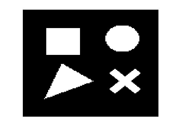
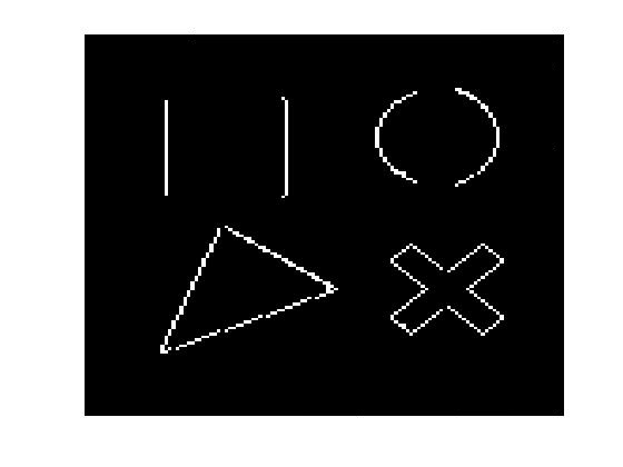
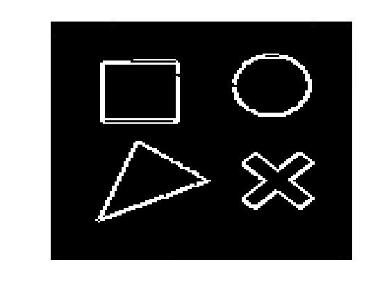
(a)                                        (b)                                       (c)

Figure 1: (a) Original image, (b) Pixels with a smoothing rate over 0.6 are indicated in white, (c) Pixels in white are those where one of the $A_{i,j},B_{i,j},C_{i,j}$ or $D_{i,j}$ values differs from the others by a factor of $50\%$ or more.

There are two approaches that have been taken to address the poor smoothing rate at edges; the first is the use of adaptive high order intergrid transfer operators [11] and the second is to apply extra smoothing steps at those edge points [8, 10, 11]. We prefer the second approach as the intergrid operators perform well generally and for ease of implementation in the current framework the second approach is best. The conventional solution when doing extra smoothing steps would be to simply implement the same smoother many more times at those edge pixels to obtain a lower smoothing rate, however we shall develop a different scheme to be used at these pixels which has an improved smoothing rate. In any case, we must first identify those pixels which contribute large amplification factors without needing to calculate $\hat{\mu}_{i,j}$ each time, which would be computationally expensive. In Table 2 we have selected the pixels in the image from Figure 1(a) which give 10 of the largest amplification factors and list the values of $A_{i,j},B_{i,j},C_{i,j}$ and $D_{i,j}$ at these pixels.

$i$	$j$	$\hat{\mu}_{i,j}$	$A_{i,j}$	$B_{i,j}$	$C_{i,j}$	$D_{i,j}$
46	23	0.9997	202	202	137391	35
45	23	0.9995	202	202	77788	35
25	23	0.9931	209	220	5545	36
42	112	0.9889	2263	1802	78959	842
44	82	0.9605	20	626	558	22

$i$	$j$	$\hat{\mu}_{i,j}$	$A_{i,j}$	$B_{i,j}$	$C_{i,j}$	$D_{i,j}$
44	112	0.9591	79987	6659	168919	6736
97	103	0.9551	3228	105968	72894	3203
80	60	0.9312	7937	424357	400718	27651
73	90	0.8756	29221	1426471	170469	21920
73	105	0.8750	321703	24343	242663	32126

Table 2: The pixels with $10$ of the largest smoothing rates with the corresponding values of $A_{i,j},B_{i,j},C_{i,j}$ and $D_{i,j}$.

A pattern emerges that at these edge pixels (jumps) at least one of the values of $A_{i,j},B_{i,j},C_{i,j}$ and $D_{i,j}$ is significantly different to the others, Figure 1(c) shows those pixels where they differ by 50% (i.e. $\max(A_{i,j},B_{i,j},C_{i,j},D_{i,j})/\min(A_{i,j},B_{i,j},C_{i,j},D_{i,j})>1.5$).

Definition 1.

We can identify the edge pixels as those where at least one of $A_{i,j},B_{i,j},C_{i,j}$ or $D_{i,j}$ differs significantly from the others, this is precisely the set of jumps in the coefficients of (6), we denote this set by $\mathcal{D}$. For the set of pixels where $A_{i,j},B_{i,j},C_{i,j}$ or $D_{i,j}$ are relatively similar we denote it as $\Omega\backslash\mathcal{D}$.

We compare the maximum and average smoothing rates over $\mathcal{D}$ and $\Omega\backslash\mathcal{D}$ below:

Smoother $$\tilde{\mu}_{\max\mathcal{D}} \tilde{\mu}_{\text{avg }\mathcal{D}} \tilde{\mu}_{\max\Omega\backslash\mathcal{D}} \tilde{\mu}_{\text{avg }\Omega\backslash\mathcal{D}}$$ GSLINE-I 0.9997 0.5121 0.7705 0.4386 (20)

We see that the maximum amplification factor over $\Omega\backslash\mathcal{D}$ of 0.7705 would mean that the number of iterations required to reduce the high-frequency errors by 90% reduces from 7675 to 9. We now focus on reducing the amplification factor for the pixels of $\mathcal{D}$.

Classifying the jumps. There are $14$ possible cases to consider where one of the coefficients $A_{i,j},B_{i,j},C_{i,j}$ or $D_{i,j}$ is relatively larger (L) or smaller (S) than the others, these are all shown below:

We can now label each pixel in $\mathcal{D}$ as one of the cases from $1$ to $14$. The choice of label $L$ or $S$ for a coefficient will be dependent on the coefficients at each pixel. Typically, if the largest coefficient is 50% larger than the smallest we group the coefficients as large or small by K-means or some other classification method. For a pixel in $\mathcal{D}$, we now look to adapt the iterative scheme (15) for each of these cases to give a scheme which has a better smoothing rate than implementing GSLINE-I directly. In the interests of brevity, we consider Case $1$ in detail and will generalise the results to other cases next.

4.1.1 An adapted iterative scheme and its LFA form

Our aim is to propose a new iteration scheme which leads to a smaller smoothing rate by the LFA. For Case 1 pixels, $A_{i,j}$ and $D_{i,j}$ are relatively small and $B_{i,j}$ and $C_{i,j}$ are relatively large. We can rewrite (15) as

$$B_{i,j}\phi_{i-1,j}+C_{i,j}\phi_{i,j+1}-S_{i,j}\phi_{i,j}=f_{i,j}-A_{i,j}\phi_{i+1,j}-D_{i,j}\phi_{i,j-1},$$

by moving the small terms to the right hand side. We now look to solve $\phi_{i-1,j},\phi_{i,j+1}$ and $\phi_{i,j}$ as a coupled system. We can rewrite this scheme, with the iteration number indicated, as

$$B_{i,j}\phi_{i-1,j}^{(k+1)}+C_{i,j}\phi_{i,j+1}^{(k+1)}-S_{i,j}\phi_{i,j}^{(k+1)}=f_{i,j}-A_{i,j}\phi_{i+1,j}^{(k)}-D_{i,j}\phi_{i,j-1}^{(k)}.$$ (22)

The amplification factor for such a scheme is

$$\hat{\mu}_{i,j}=\max_{\theta_{1},\theta_{2}}\mu(\theta_{1},\theta_{2})=\max_{\alpha_{1},\alpha_{2}}\frac{|A_{i,j}e^{{\bf i}\alpha_{1}}+D_{i,j}e^{-{\bf i}\alpha_{2}}|}{|S_{i,j}-B_{i,j}e^{-{\bf i}\alpha_{1}}-C_{i,j}e^{{\bf i}\alpha_{2}}|},$$ (23)

derived as in §3.4. In fact, we see the following improvements to the maximum and average smoothing rates for all of the Case 1 pixels by using the adapted iterative scheme (22) rather than the GSLINE-I smoother in (13)

$$\tilde{\mu}_{\max}=0.9863,\ \tilde{\mu}_{\text{avg}}=0.7174\quad\Longrightarrow\quad\tilde{\mu}_{\max}=0.7324,\ \tilde{\mu}_{\text{avg}}=0.3013$$

Reducing the smoothing rate from 0.9863 to 0.7324 is dramatic; exemplified by the fact that to reduce high-frequency errors by 90% for Case 1 pixels with GSLINE-I we would have required 167 iterations but now we need just 8. Hence, now we know that the scheme (22) gives us a better smoothing rate than GSLINE-I at these pixels.

4.1.2 Adapted schemes for all cases of (21) and their rates by LFA

Using the central idea of lagging the small terms in (21) (between $1$ and $3$ terms), we can derive adapted schemes for all cases in the same manner as for Case 1 previously. In Table 3 we give the comparison of the maximum smoothing rate of GSLINE-I, $\mu_{GSLINE}$, with the maximum smoothing rate of the adapted schemes $\mu_{adapted_{1}}$.

Case #	$\mu_{GSLINE}$	$\mu_{adapted_{1}}$
1	0.9863	0.7324	$\diamondsuit$
2	0.6259	0.8515	$\diamondsuit$
3	0.9900	0.7418	$\diamondsuit$
4	0.6408	0.7415	$\diamondsuit$
5	0.7105	1.0000	$\Box$
6	0.9524	1.0000	$\Box$
7	0.9592	0.9536	$\diamondsuit$

Case #	$\mu_{GSLINE}$	$\mu_{adapted_{1}}$
8	0.9997	0.9569	$\diamondsuit$
9	0.9481	0.9426	$\diamondsuit$
10	0.8935	0.9640	$\diamondsuit$
11	0.2693	0.2693	$\spadesuit$
12	0.7729	0.2663	$\spadesuit$
13	0.9865	0.2704	$\spadesuit$
14	0.5993	0.2706	$\spadesuit$

Table 3: Comparison of the maximum amplification factors using GSLINE-I and the adapted iterative schemes for each case. The $\Box$-cases are the decoupled cases which give a rate of precisely 1, as remarked, the $\diamondsuit$-cases have minor or no improvement in the smoothing rate and the $\spadesuit$-cases have a good final rate.

The results from Table 3 fall into $3$ categories:

• $\spadesuit$-cases, where only one term is lagged and the improvements are remarkable. This gives a promising indication that the lagging of particular terms in certain cases can improve the smoothing rate. This motivates our next step.

• $\diamondsuit$-cases, where either $2$ or $3$ terms are lagged. We see either only a minor improvement to an already high rate or the rate has actually worsened.

• $\Box$-cases, where $2$ terms are lagged and we see the worst results: a smoothing rate of 1.0000 is attained for cases $5,6$ in Table 3. Below we prove analytically that for Case $6$ pixels the smoothing rate when using the adapted scheme will always be precisely 1.

  Case $6$ pixels have the LFA form $\hat{\mu}_{i,j}=\max_{\alpha_{1},\alpha_{2}}\frac{|A_{i,j}e^{{\bf i}\alpha_{1}}+B_{i,j}e^{-{\bf i}\alpha_{1}}|}{|S_{i,j}-C_{i,j}e^{{\bf i}\alpha_{2}}-D_{i,j}e^{-{\bf i}\alpha_{2}}|},$ and we see a decoupling in the maximisation with respect to $\alpha_{1}$ and $\alpha_{2}$ which allows us to rewrite this as

  $\begin{gathered}\begin{aligned} \hat{\mu}_{i,j}&=\frac{\max\limits_{\alpha_{1}}\Big{|}A_{i,j}e^{{\bf i}\alpha_{1}}+B_{i,j}e^{-{\bf i}\alpha_{1}}\Big{|}}{\min\limits_{\alpha_{2}}\Big{|}S_{i,j}-C_{i,j}e^{{\bf i}\alpha_{2}}-D_{i,j}e^{-{\bf i}\alpha_{2}}\Big{|}}=\frac{\max\limits_{\alpha_{1}}\Big{|}(A_{i,j}+B_{i,j})\cos(\alpha_{1})+{\bf i}(A_{i,j}-B_{i,j})\sin(\alpha_{1})\Big{|}}{\min\limits_{\alpha_{2}}\Big{|}\left[A_{i,j}+B_{i,j}+C_{i,j}(1-\cos(\alpha_{2}))+D_{i,j}(1-\cos(\alpha_{2}))\right]+{\bf i}(C_{i,j}-D_{i,j})\sin(\alpha_{2})\Big{|}}\\ \rule{0.0pt}{30.1388pt}&=\frac{\sqrt{\max\limits_{\alpha_{1}}\Big{[}A_{i,j}^{2}+B_{i,j}^{2}+2A_{i,j}B_{i,j}cos(2\alpha_{1})\Big{]}}}{\sqrt{\min\limits_{\alpha_{2}}\Big{[}\left[A_{i,j}+B_{i,j}+C_{i,j}(1-\cos(\alpha_{2}))+D_{i,j}(1-\cos(\alpha_{2}))\right]^{2}+(C_{i,j}-D_{i,j})^{2}\sin(\alpha_{2})^{2}\Big{]}}}\quad=\quad\frac{(A_{i,j}+B_{i,j})^{2}}{(A_{i,j}+B_{i,j})^{2}}=1,\\ \end{aligned}\end{gathered}$

  attained at $(\alpha_{1},\alpha_{2})=(-\pi,0)\in[-\pi,\pi)^{2}\backslash[-\frac{\pi}{2},\frac{\pi}{2})^{2}$. Similarly we have $\hat{\mu}_{i,j}=1$ for Case $5$ too.

  We claim that it is necessary to have both of $\alpha_{1}$ and $\alpha_{2}$ in the numerator or denominator of the LFA formulation to ensure a low smoothing rate. We note that for Cases $5$ and $6$ this is not the case.

We now focus on improving the $\diamondsuit$-cases and the Case 8 in particular and its LFA to motivate us on how to proceed i.e. to see whether an alternative adaptation to the iterative scheme gives a better smoothing rate. The results apply to $\Box$-cases also.

Improving the adapted scheme for Case 8. A pixel which is labelled as Case $8$ is one where $A_{i,j},B_{i,j},D_{i,j}$ are relatively small and $C_{i,j}$ is relatively large. Using the previous method we would devise a scheme where the terms with coefficients $A_{i,j},B_{i,j},D_{i,j}$ would be lagged at time step $k$ and the term with coefficient $C_{i,j}$ would be updated to time step $k+1$. We pick the particular Case 8 pixel from Table 2 which has the worst smoothing rate and in Figure 2 we look at the smoothing rate for the scheme (15) with different coefficients lagged.

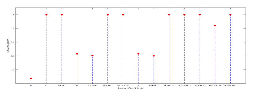
Figure 2: Comparison of the smoothing rate for the Case 8 pixel with the worst smoothing rate when different coefficient terms are lagged. In this case, $A_{i,j}=202,B_{i,j}=202,C_{i,j}=137391$ and $D_{i,j}=35$ (Table 2).

This shows that the best rate is achieved when just the smallest of the coefficients ($D_{i,j}$) is lagged. Even the lagging of two of the smallest coefficients gives an improvement on lagging all three. This gives some indication that the smoothing rate is best when the smallest coefficient is lagged and this has proven to be the case in every one of the many examples which the authors have tried. It would be an interesting piece of future work to prove that this must be true analytically.

Hence we propose to lag just the smallest of the coefficients in a modified scheme for all cases.

4.1.3 Improved adapted schemes for all cases

We re-consider the $\Diamond$ and $\Box$-cases which have more than one relatively small coefficient. Lagging only the smallest coefficient, the LFA forms simplify to those of Cases 11–14 and we expect major improvements. In Table 4 we compare the maximum smoothing rate of GSLINE-I, $\mu_{GSLINE}$, for these cases with the maximum smoothing rate of an improved, adapted iterative scheme which lags only the smallest coefficient $\mu_{adapted_{2}}$.

Case #	$\mu_{GSLINE}$	$\mu_{adapted_{2}}$
1	0.9863	0.4467
2	0.6259	0.4398
3	0.9900	0.4280
4	0.6408	0.4468
5	0.7105	0.4659
6	0.9524	0.4547
7	0.9592	0.4789

Case #	$\mu_{GSLINE}$	$\mu_{adapted_{2}}$
8	0.9997	0.4779
9	0.9481	0.4716
10	0.8935	0.4749
11	0.2693	0.2693
12	0.7729	0.2663
13	0.9865	0.2704
14	0.5993	0.2706

Table 4: Comparison of the maximum amplification factors using GSLINE-I and the adapted iterative schemes for each case with just the smallest coefficient term lagged.

As expected, there is a significant improvement in the smoothing rate in all cases when we lag just the smallest coefficient, it also makes implementation faster as we now consider just 4 cases of possible lagged coefficients rather than 14 and therefore have only 4 iterative schemes to consider. Taking our guidance from these results, we propose two hybrid smoothers which both perform standard smoothing iterations on pixels of $\Omega\backslash\mathcal{D}$ and perform non-standard adapted iterative schemes on the pixels in $\mathcal{D}$.

Based on the above pixel-wise motivating tests, we now present two iterative strategies for our new smoothers. The first smoother is natural: for each pixel $(i,j)$, in $\mathcal{D}$, all of the directly connected neighbouring pixels are collectively updated except the term with the smallest coefficient. That is, Hybrid Smoother 1 uses block structure Vanka-type smoothing schemes [32, 35] to update the pixels in $\mathcal{D}$. The potential drawback is that previously updated pixels may enter to the next group of (potentially multiple) updates, making subsequent analysis intractable. Hence our second smoother, denoted by ‘Hybrid Smoother 2’, incorporates partial line smoothing operations at pixels in $\mathcal{D}$ and only pixels that are the same line as $(i,j)$ are updated. This line by line approach facilitates subsequent analysis.

4.2.   Hybrid Smoother 1

Our first hybrid smoother updates blocks of pixels at each update, these blocks may overlap. This is an overlapping block smoother of Vanka-type [32, 35]. Once again we start with the set $\mathcal{D}$ of pixels with jumping coefficients. For brevity, we will detail the derivation of the iterative scheme for pixels in $\mathcal{D}$ for which $A_{i,j}$ is smallest. We will then state the schemes for the other laggings (derived in the same manner).

$A_{i,j}$ lagged. The lagging of coefficient $A_{i,j}$ in equation (15) gives rise to the iterative scheme

$$A_{i,j}\phi_{i+1,j}^{(k)}+B_{i,j}\phi_{i-1,j}^{(k+1)}+C_{i,j}\phi_{i,j+1}^{(k+1)}+D_{i,j}\phi_{i,j-1}^{(k+1)}-S_{i,j}\phi_{i,j}^{(k+1)}=f_{i,j},$$ (24)

We are solving for $\phi_{i-1,j},\phi_{i,j+1},\phi_{i,j-1}$ and $\phi_{i,j}$ simultaneously and as we have only one equation, we need three more. We get these by considering (15) at the pixels $(i-1,j)$ and $(i,j+1)$ and $(i,j-1)$, which gives us the three equations

$$\begin{gathered}B_{i,j}\phi_{i,j}-S_{i-1,j}\phi_{i-1,j}=f_{i-1,j}-B_{i-1,j}\phi_{i-2,j}-C_{i-1,j}\phi_{i-1,j+1}-D_{i-1,j}\phi_{i-1,j-1},\\ C_{i,j}\phi_{i,j}-S_{i,j+1}\phi_{i,j+1}=f_{i,j+1}-A_{i,j+1}\phi_{i+1,j+1}-B_{i,j+1}\phi_{i-1,j+1}-C_{i,j+1}\phi_{i,j+2},\\ D_{i,j}\phi_{i,j}-S_{i,j-1}\phi_{i,j-1}=f_{i,j-1}-A_{i,j-1}\phi_{i+1,j-1}-B_{i,j-1}\phi_{i-1,j-1}-D_{i,j-1}\phi_{i,j-2},\\ \end{gathered}$$

which have been rearranged to have the $\phi_{i-1,j},\phi_{i,j+1},\phi_{i,j-1}$ and $\phi_{i,j}$ terms on the left hand side. So, using these along with (24) we obtain the system (25).

Scheme with $A_{i,j}$ lagged:

$$\leavevmode\resizebox{422.77661pt}{}{$\left(\begin{array}[]{cccc}-S_{i,j}&B_{i,j}&C_{i,j}&D_{i,j}\\ B_{i,j}&-S_{i-1,j}&0&0\\ C_{i,j}&0&-S_{i,j+1}&0\\ D_{i,j}&0&0&-S_{i,j-1}\\ \end{array}\right)\cdot\left(\begin{array}[]{c}\phi_{i,j}\\ \phi_{i-1,j}\\ \phi_{i,j+1}\\ \phi_{i,j-1}\\ \end{array}\right)=\left(\begin{array}[]{c}f_{i,j}-A_{i,j}\phi_{i+1,j}\\ f_{i-1,j}-C_{i-1,j}\phi_{i-1,j+1}-D_{i-1,j}\phi_{i-1,j-1}-B_{i-1,j}\phi_{i-2,j}\\ f_{i,j+1}-A_{i,j+1}\phi_{i+1,j+1}-B_{i,j+1}\phi_{i-1,j+1}-C_{i,j+1}\phi_{i,j+2}\\ f_{i,j-1}-A_{i,j-1}\phi_{i+1,j-1}-B_{i,j-1}\phi_{i-1,j-1}-D_{i,j-1}\phi_{i,j-2}\\ \end{array}\right)$}.$$ (25)

This system is strictly diagonally dominant and follows the guidance in [34] that collective update schemes are better for jumping coefficients. This system also has an arrow structure in the matrix and can be solved very quickly (in 24 operations).

4.2.1 The adapted iterative schemes for other cases

Below are the adapted iterative schemes for the cases when $B_{i,j},C_{i,j}$ or $D_{i,j}$ are lagged, derived in the same manner as previously when $A_{i,j}$ was lagged.

Scheme with $B_{i,j}$ lagged:

$$\leavevmode\resizebox{422.77661pt}{}{$\left(\begin{array}[]{cccc}-S_{i,j}&A_{i,j}&C_{i,j}&D_{i,j}\\ A_{i,j}&-S_{i+1,j}&0&0\\ C_{i,j}&0&-S_{i,j+1}&0\\ D_{i,j}&0&0&-S_{i,j-1}\\ \end{array}\right)\cdot\left(\begin{array}[]{c}\phi_{i,j}\\ \phi_{i+1,j}\\ \phi_{i,j+1}\\ \phi_{i,j-1}\\ \end{array}\right)=\left(\begin{array}[]{c}f_{i,j}-B_{i,j}\phi_{i-1,j}\\ f_{i+1,j}-C_{i+1,j}\phi_{i+1,j+1}-D_{i+1,j}\phi_{i+1,j-1}-A_{i+1,j}\phi_{i+2,j}\\ f_{i,j+1}-A_{i,j+1}\phi_{i+1,j+1}-B_{i,j+1}\phi_{i-1,j+1}-C_{i,j+1}\phi_{i,j+2}\\ f_{i,j-1}-A_{i,j-1}\phi_{i+1,j-1}-B_{i,j-1}\phi_{i-1,j-1}-D_{i,j-1}\phi_{i,j-2}\\ \end{array}\right)$}.$$ (26)

Scheme with $C_{i,j}$ lagged:

$$\leavevmode\resizebox{422.77661pt}{}{$\left(\begin{array}[]{cccc}-S_{i,j}&A_{i,j}&B_{i,j}&D_{i,j}\\ A_{i,j}&-S_{i+1,j}&0&0\\ B_{i,j}&0&-S_{i-1,j}&0\\ D_{i,j}&0&0&-S_{i,j-1}\\ \end{array}\right)\cdot\left(\begin{array}[]{c}\phi_{i,j}\\ \phi_{i+1,j}\\ \phi_{i-1,j}\\ \phi_{i,j-1}\\ \end{array}\right)=\left(\begin{array}[]{c}f_{i,j}-C_{i,j}\phi_{i,j+1}\\ f_{i+1,j}-C_{i+1,j}\phi_{i+1,j+1}-D_{i+1,j}\phi_{i+1,j-1}-A_{i+1,j}\phi_{i+2,j}\\ f_{i-1,j}-C_{i-1,j}\phi_{i-1,j+1}-D_{i-1,j}\phi_{i-1,j-1}-B_{i-1,j}\phi_{i-2,j}\\ f_{i,j-1}-A_{i,j-1}\phi_{i+1,j-1}-B_{i,j-1}\phi_{i-1,j-1}-D_{i,j-1}\phi_{i,j-2}\\ \end{array}\right)$}.$$ (27)

Scheme with $D_{i,j}$ lagged:

$$\leavevmode\resizebox{422.77661pt}{}{$\left(\begin{array}[]{cccc}-S_{i,j}&A_{i,j}&B_{i,j}&C_{i,j}\\ A_{i,j}&-S_{i+1,j}&0&0\\ B_{i,j}&0&-S_{i-1,j}&0\\ C_{i,j}&0&0&-S_{i,j+1}\\ \end{array}\right)\cdot\left(\begin{array}[]{c}\phi_{i,j}\\ \phi_{i+1,j}\\ \phi_{i-1,j}\\ \phi_{i,j+1}\\ \end{array}\right)=\left(\begin{array}[]{c}f_{i,j}-D_{i,j}\phi_{i,j-1}\\ f_{i+1,j}-C_{i+1,j}\phi_{i+1,j+1}-D_{i+1,j}\phi_{i+1,j-1}-A_{i+1,j}\phi_{i+2,j}\\ f_{i-1,j}-C_{i-1,j}\phi_{i-1,j+1}-D_{i-1,j}\phi_{i-1,j-1}-B_{i-1,j}\phi_{i-2,j}\\ f_{i,j+1}-A_{i,j+1}\phi_{i+1,j+1}-B_{i,j+1}\phi_{i-1,j+1}-C_{i,j+1}\phi_{i,j+2}\\ \end{array}\right)$}.$$ (28)

4.2.2 Implementing Hybrid Smoother 1

To minimise grid sweeps and ensure that all pixels are covered, we use the following pseudo-algorithm for Hybrid Smoother 2:

1. Perform GSLINE-I on all lines in the image.

2. For each pixel in $\mathcal{D}$, perform the appropriate scheme of (25)–(28).

We justify the choice of GSLINE-I in step I as it is the recommended smoothing scheme for a problem with jump coefficients [34]. Note that the schemes in II can overlap the same pixels several times due to the collective updates.

Algorithm 2. In future discussion, when we use the Hybrid Smoother 1 in the Full Approximation Scheme, we will call this Algorithm 2.

4.3.   Hybrid Smoother 2

Our second hybrid smoother first groups pixels in $\mathcal{D}$ by whether $A_{i,j}$, $B_{i,j}$, $C_{i,j}$ or $D_{i,j}$ are the smallest and then by the line they are on. We then perform partial line updates on these groups for $A_{i,j}$, $B_{i,j}$, $C_{i,j}$ or $D_{i,j}$ in sequence along with individual pixel updates on the other pixels, this avoids the overlap encountered in Hybrid Smoother 1. We note that for pixels in $\Omega\backslash\mathcal{D}$ the LFA tells us that the smoothing rate is acceptable (maximum 0.7705) and therefore we design a smoother which performs cheap GSLEX-I iterations at the pixels of $\Omega\backslash\mathcal{D}$ and performs the lagged scheme on the other pixels. We focus initially on how we propose implementing this for the pixels in $\mathcal{D}$ with $A_{i,j}$ lagged and then we generalise the idea to the laggings of $B_{i,j},C_{i,j}$ and $D_{i,j}$.

Scheme with $A_{i,j}$ lagged. Suppose we focus on a pixel $(i,j)\in\mathcal{D}$ which has coefficient $A_{i,j}$ the smallest. If we lag the $A_{i,j}$ the smoothing rate at this pixel is

$$\hat{\mu}_{i,j}=\max_{(\alpha_{1},\alpha_{2})\in[-\pi,\pi)^{2}\backslash[-\frac{\pi}{2},\frac{\pi}{2})^{2}}\left|\frac{A_{i,j}e^{{\bf i}\alpha_{1}}}{B_{i,j}e^{-{\bf i}\alpha_{1}}+C_{i,j}e^{{\bf i}\alpha_{2}}+D_{i,j}e^{-{\bf i}\alpha_{2}}-S_{i,j}}\right|$$

which is precisely the smoothing rate for a line smoother updating from the top row to the bottom row. In the majority of cases, if pixel $A_{i,j}$ is the smallest, we find that many adjacent pixels on that line also have $A_{i,\cdot}$ the smallest. So we can perform a partial line smoothing on these pixels.

In this new strategy, the only technical issue to address is that, at a pixel $(i,j)$ in set $\mathcal{D}$, the lagged coefficient (here $A_{i,j}$) must be a previously updated pixel in this iteration otherwise we cannot avoid multiple updates (as with Hybrid Smoother 1) within one smoothing iteration. Our proposed solution is to view a group of adjacent pixels in set $\mathcal{D}$ whose smallest coefficient is $A_{i,j}$ (shown as starred pixels in Figure 3) and sit on a line as a superpixel and to update together with their $A_{i,j}$ terms lagged. If the superpixel is comprised of a single pixel, we set its immediate neighbour pixel (here $(i,j+1)$) as a starred pixel so the group is of size 2. All other pixels in set $\mathcal{D}$ (without smallest coefficient $A_{i,j}$) and those not in $\mathcal{D}$ are treated as normal pixels (non-starred) and are relaxed by the GSLEX-1 formula. Hence in each smoothing step, starred and non-starred pixels are only updated once.

In Figure 3 we illustrate how this proposed algorithm would update the pixels, steps I–VI represent one iteration of the smoother on the $5\times 5$ grid. The starred pixels represent those pixels which have $A_{i,j}$ the smallest. The algorithm proceeds as follows:

1. We identify the pixels in $\mathcal{D}$ which have $A_{i,j}$ the smallest (indicated by a star).

2. Perform GSLEX-I on all non-starred pixels.

3. Collective partial line update on adjacent starred pixels.

4. Perform GSLEX-I again on all non-starred pixels.

5. If a single starred pixel is found, update collectively with the immediate neighbour.

6. Perform GSLEX-I again on all non-starred pixels.

I

II

III

IV

V

VI

Figure 3: Illustration of the hybrid algorithm for a pixel grid. Each image represents one step of the algorithm, grey cells are yet to be updated. The star pixels are pixels in $\mathcal{D}$ with $A_{i,j}$ smallest. Green represents the update by GSLEX-I and the yellow pixels are the partial line smoothing updates.

4.3.1 The adapted iterative schemes for other cases

We previously focussed on the case for $A_{i,j}$ being lagged and now discuss other components of our iterative scheme to cover the cases of $B_{i,j},C_{i,j}$ and $D_{i,j}$ being lagged.

Crucially, to ensure that the scheme agrees with the LFA we must change the direction of update between the schemes for updating $A_{i,j}$, $B_{i,j}$, $C_{i,j}$ and $D_{i,j}$. For example, if we are lagging $B_{i,j}$ pixels we must update from the bottom-right corner to the top-left moving along rows right to left and from the bottom row to the top row. In Figure 4 we show the order in which the pixels should be updated for each lagging.

These sweeps in other directions are required to help those pixels in $\mathcal{D}$ that were treated as non-starred pixels due to their smallest coefficients not being considered in the other sweeps. That is to say, each of 4 sweeps takes care of one type of alignment of the smallest coefficients (of course there are no other directions to consider). Consequently, after all 4 sweeps, the compounded smoothing rate at each pixel is small because we have ensured that one of the four multiplying factors is small while the other three are no more than 1.

The broad algorithm (I–VI) is the same in these cases as for the case of $A_{i,j}$ lagged; we identify the pixels which are of that case, perform GSLEX-I on all others and partial line updates on identified pixels.

Hybrid Smoother 2 performs 4 sweeps of the grid, each repeating the above I–V and differing only in update order and assignment of starred pixels. In Figure 4 we display the order in which the pixels and superpixels should be updated for each lagging.

${\bm{A}_{i,j}}$ Lagged

${\bm{B}_{i,j}}$ Lagged

${\bm{C}_{i,j}}$ Lagged

${\bm{D}_{i,j}}$ Lagged

Figure 4: Illustration of the hybrid algorithm for a pixel grid. The star pixels are pixels in $\mathcal{D}$ with $A_{i,j}$ smallest. Green represents the update by GSLEX-I and the yellow pixels are the partial line smoothing updates.

4.3.2 Implementing Hybrid Smoother 2

To ensure all laggings are considered, we sweep for $A_{i,j}$, $B_{i,j}$, $C_{i,j}$ and $D_{i,j}$ in this order, performing steps (I–VI) on each sweep. These schemes are performed on all pixels in $\mathcal{D}$ and we see from Table 4 that the maximum smoothing rate over $\mathcal{D}$ falls from 0.9997 to 0.4789. Therefore to reduce high-frequency errors by 90%, with GSLINE-I this would have needed 7675 iterations but with the adapted iterative schemes we need only 4.

To ensure that all cases are considered, we design a hybrid smoother for which one outer iteration includes four sweeps of the image domain. In the first sweep we lag $A_{i,j}$, then in the second $B_{i,j}$ and so on. We note, for example, that in the sweep with $A_{i,j}$ lagged, then the pixels with coefficient $B_{i,j}$ smallest have a poor smoothing rate, however on the $B_{i,j}$ sweep the rate is good for these pixels and poor for those where we have $A_{i,j}$ smallest. However, as the effects compound multiplicatively, after each outer iteration, the smoothing rate at pixels in $\mathcal{D}$ is good and for $\Omega\backslash\mathcal{D}$ is also good as these have had 4 GSLEX-I iterations.

We now consider the smoothing rates we can attain with this smoother. Firstly, for the Rada-Chen model [31], using (20) we see that the maximum smoothing rate in each outer iteration of the smoother on $\Omega\backslash\mathcal{D}$ is approximately $0.7705^{4}=0.3524$. By performing the adapted iterative schemes on $\mathcal{D}$ we have a maximum smoothing rate of 0.4789 (Table 4) in a single sweep. We know that the rate for GSLEX-I is poor for these pixels in $\mathcal{D}$ (close to 1) so the main reduction in error occurs when we perform the adapted scheme with the appropriate lagging. Therefore the maximum smoothing rate in one outer iteration of the smoother is approximately 0.4789, which is very good. One consideration we must make is that the domain is covered $4$ times in each outer iteration, which could be computationally intensive for a large number of smoothing steps. Typically we find that for non-linear problems the number of overall sweeps of the grid is around 10-20 (see, for example, [11, 39]) for the smoother, therefore we suggest 2 outer iterations (8 grid sweeps) which gives an impressive smoothing rate and is acceptable computationally.

Adaptive iterative schemes applied to the Spencer-Chen model [33]. We applied Hybrid Smoother $2$ to the Spencer-Chen model. In this case using just GSLINE-I we have a maximum smoothing rate of 0.9990 but using the new smoother, the maximum smoothing rate falls to 0.5032. Therefore, to reduce errors by 90% we need $4$ iterations rather than $2302$. This is a further indication that the technique of using the partial line smoothers at the pixels with jumps in the coefficients is a good way to reduce the maximum smoothing rate of the smoother and the idea transfers to other models.

Improved smoothing rates for other images. We now show how the maximum smoothing rate for Hybrid Smoother $2$ is smaller than GSLINE-I for several images with different levels of Gaussian noise. We compare to GSLINE-I as this is the recommended standard smoother for problems with jumping coefficients. We denote the corresponding maximum smoothing rates as $\mu_{GSLINE-I}$ and $\mu_{GSHYBRID}$ respectively. Results obtained previously are just for the clean image in Figure 1(a). Here we compare the smoothing rates for noisy versions of this image and also of those in Figure 5.

Image	$\mu_{GSLINE-I}$	$\mu_{HYBRID}$
Figure 1(a) + 1% Noise	0.9743	0.4891
Figure 1(a) + 5% Noise	0.9851	0.4815
Problem 1	0.9960	0.4532
Problem 1 + 1% Noise	0.9900	0.4749
Problem 1 + 5% Noise	0.9991	0.4789

Image	$\mu_{GSLINE-I}$	$\mu_{HYBRID}$
Problem 2	0.9999	0.4736
Problem 2 + 1% Noise	0.9988	0.4886
Problem 2 + 5% Noise	0.9934	0.4518
Problem 3	0.9999	0.4829
Problem 3 + 1% Noise	0.9999	0.4863
Problem 3 + 5% Noise	0.9999	0.4841

Table 5: Comparison of the maximum smoothing rates for GSLINE-I and Hybrid Smoother $2$ for various images.

Algorithm 3. In future discussion, we refer to the Full Approximation Scheme using Hybrid Smoother 2 as Algorithm 3.

5.   Numerical Experiments

In this section we show two types of numerical experiments: comparisons with the current best methods and analysis of the complexity of Algorithms 2 and 3. Results have been obtained for many artificial and real images but we restrict to the images shown in Figure 5. We show real images as these are of most interest for the application of selective segmentation.

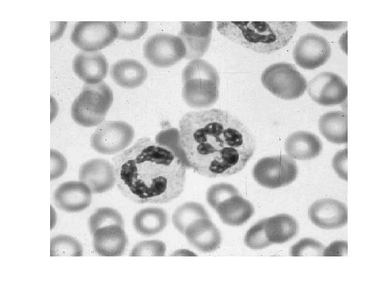
Problem 1

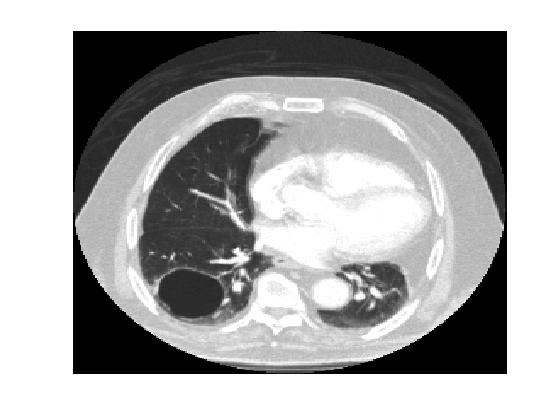
Problem 2

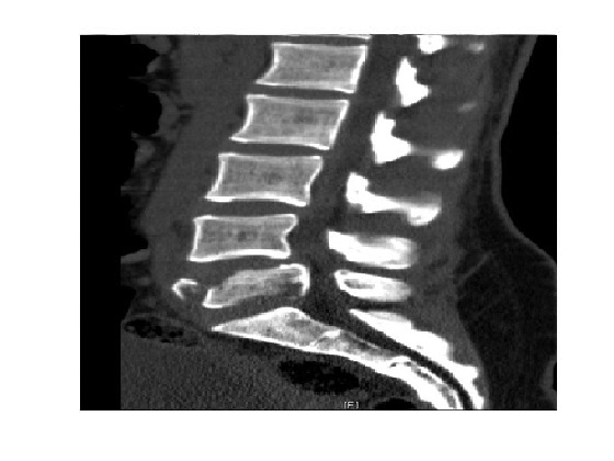
Problem 3

Figure 5: The test images used in this section for the experiments.

The Rada-Chen and Spencer-Chen models we look at are non-convex and we therefore need the initialisation to be close to the final solution. Thankfully this can be achieved by setting the initial contour as the boundary of the polygon formed from the user selected points in $\mathcal{S}$. For examples of such user defined points, see Figure 7.

Parameter Choices. The values of $c_{1}$ and $c_{2}$, being the average intensities inside and outside of the contour, are updated at the end of each multigrid iteration - the initial values are set to the average inside and outside the initial contour. We fix $\mu=1/2$, $\lambda_{1}=\lambda_{2}=10^{-4}$, $\nu=1$ (for the Rada-Chen model) and $\theta=1$ (for the Spencer-Chen model). In all experiments we use a V-cycle, i.e. fix $\gamma=1$.

Number of Smoothing Steps. To decide how many smoothing steps were required in Algorithms 1, 2 and 3, we performed experiments to see how the number of smoothing steps impacted the number of multigrid cycles for convergence. As the number of smoothing steps increases, the number of cycles decreases and plateaus. We fix the number of smoothing steps for each algorithm as the number required for the number of multigrid cycles to first plateau. In Figure 6 we demonstrate how the number of multigrid cycles required for convergence changes with the number of smoothing steps and how we choose the optimal number of pre- and post-smoothing steps ($\nu_{1}$ and $\nu_{2}$). In all tests we use 100 iterations of the exact solver (AOS) on the coarsest level.

Figure 6: The number of smoothing steps plotted against the number of multigrid cycles required to achieve convergence for Algorithm 3 on Problem 1. Guided by this, we choose 3 smoothing steps as the gain plateau’s at this point.

Using this technique, we fix the smoothing steps for Algorithms 1, 2 and 3 as $\nu_{1}=\nu_{2}=$ 5, 3 and 3 respectively.

5.1.   Comparison of Algorithm $2$ and Algorithm $3$ with AOS

In this section we compare the speed of the proposed Algorithms 2 and 3 with AOS. We use the image from Problem 1 and scale this to different resolutions. The methods both use the standard stopping criteria $\frac{||\phi^{(k+1)}-\phi^{(k)}||_{2}}{||\phi^{(k)}||_{2}}<\eta$, where $\eta$ is a small tolerance parameter. In Table 6 we see that Algorithm $3$ is faster to reach the stopping criteria (with $\eta=10^{-4}$) than Algorithm $2$ and that both are faster than AOS for all but the smallest resolution image. We see that as the image size grows larger, performance is significantly better. One key aspect of Algorithms $2$ and $3$ is that we have the expected ratio for an $\mathcal{O}(N)$ method (in 2D) of 4 and hence an optimal complexity multigrid method. We also see that the multigrid method has a stable number of overall iterations, whereas with the AOS method, the iteration number grows as the image size grows. Finally, we see that, although it converges faster overall, the cost per MG cycle is larger for Algorithm $3$ than $2$. This is due to a higher number of grid sweeps being required in the smoothing steps, however we believe that with improved and optimised coding of the smoother the performance of Algorithm $3$ can be increased to achieve far faster convergence than that of Algorithm $2$.

Image size	Number of Unknowns, $N$	AOS		Algorithm 2			Algorithm 3
		Iter	CPU Time (s)	Iter	CPU Time (s)	CPU Ratio	Iter	CPU Time (s)	CPU Ratio
256 $\times$ 256	65536	32	3.2	4	3.1	-	4	8.8	-
512 $\times$ 512	262144	39	17.3	5	11.6	3.7	3	15.0	1.7
1024 $\times$ 1024	1048576	48	123.5	5	44.0	3.8	3	43.8	2.9
2048 $\times$ 2048	4194304	60	759.2	5	174.2	4.0	3	174.1	4.0
4096 $\times$ 4096	16777216	75	8632.4	5	725.9	4.2	3	688.2	4.0
8192 $\times$ 8192	67108864	*	*	5	2952.2	4.1	3	2766.9	4.0

Table 6: For an image of size $N=m\times n$, we show a comparison of the number of iterations and the associated CPU times to achieve the same results for the Rada-Chen model for AOS and Algorithms $2$ and $3$. ‘*’ indicates that the runtime exceeded 24 hours.

5.2.   Comparison of Algorithms 1, 2 and 3

We now look to see the practical gains from improving the smoother, i.e. the improved smoothing rate of Algorithm 3 should translate into a faster convergence rate [27].

Definition 2.

In both Algorithms 2 and 3 we must identify the set $\mathcal{D}$, being pixels at which the coefficients vary significantly. To do this we compute the minimum multiplicative factor between the largest and smallest of the coefficients $A_{i,j},B_{i,j},C_{i,j},D_{i,j}$ (see §4.1). We will denote the minimum multiplicative factor by $\Sigma$.

For completion, we will compare Algorithms 2 and 3 to Algorithm 1 for a range of $\Sigma$ values. The algorithms are all used to segment the image in Figure 1(a), with fine grid $1024^{2}$ and coarse grid $32^{2}$ and $\eta=10^{-4}$ (all parameters are as earlier in §5).

Level set energies. In Table 7 we give the energy of the level set at the end of each multigrid cycle for the Rada-Chen model for Algorithms 1, 2 and 3 for various $\Sigma$ values. The rows are ordered in descending order.

	Iteration
	1	2	3	4	5	6	7
Algorithm 1	2.4687	1.9333	1.9271	1.9253	1.9247	1.9241	1.9236
Algorithm 2 ($\Sigma=16$)	2.4684	1.9333	1.9264	1.9244	1.9238	-	-
——–"——– ($\Sigma=8$)	2.4683	1.9321	1.9251	1.9242	1.9235	-	-
——–"——– ($\Sigma=4$)	2.4683	1.9302	1.9242	1.9237	1.9226	-	-
——–"——– ($\Sigma=2$)	2.4563	1.9269	1.9214	1.9207	1.9199	-	-
Algorithm 3 ($\Sigma=16$)	2.4300	1.9185	1.9180	-	-	-	-
——–"——– ($\Sigma=8$)	2.4253	1.9171	1.9166	-	-	-	-
——–"——– ($\Sigma=4$)	2.4184	1.9167	1.9164	-	-	-	-
——–"——– ($\Sigma=2$)	2.4136	1.9165	1.9163	-	-	-	-

Table 7: Level set energies ($\times 10^{5}$) after each multigrid iteration of Algorithms 1, 2 and 3 (for varying $\Sigma$) on the image in Figure 1(a) + 10% Gaussian noise. A dash indicates convergence before iteration number was reached.

Firstly, we see that Algorithm 3 converges in $3$ cycles, where Algorithm 2 converges in $5$ and Algorithm 1 converges in $7$ cycles. Secondly, we notice that the energy is smallest for Algorithm $3$ and Algorithm $2$ gives a lower energy than Algorithm $1$ (for all $\Sigma$ values). Finally, we notice that as $\Sigma$ gets smaller (and the number of pixels in $\mathcal{D}$ increases), the energy of the level set at each cycle is smaller. This is all in agreement with the theoretical understanding of the smoothers, that they should give a small rate on the pixels in $\mathcal{D}$, and by increasing the size of $\mathcal{D}$ convergence improves.

Recommended Algorithm. The CPU timings for Algorithm 3 are the best of the three algorithms (Table 6). The level set energies are also the lowest for Algorithm 3 (Table 7) at each iteration. It performs the best at tackling the PDEs which have many discontinuous coefficients and the experimental results are in agreement with the theory in §4.3. We therefore recommend Algorithm $3$ to achieve a fast solution to the Rada-Chen and Spencer-Chen selective segmentation models.

Algorithm 3 Results. In Figure 7 we briefly show the results of Algorithm $3$ applied to the test images for the Rada-Chen model shown in Figure 1(a) and Figure 5 with $\eta=10^{-4}$.

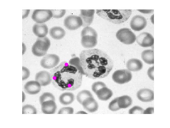
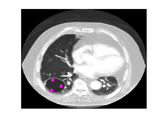
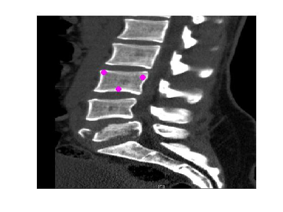
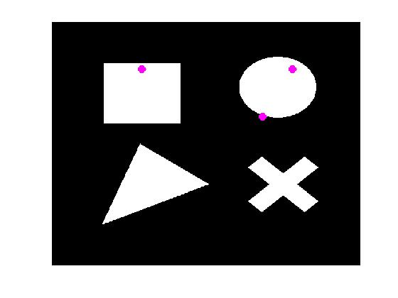
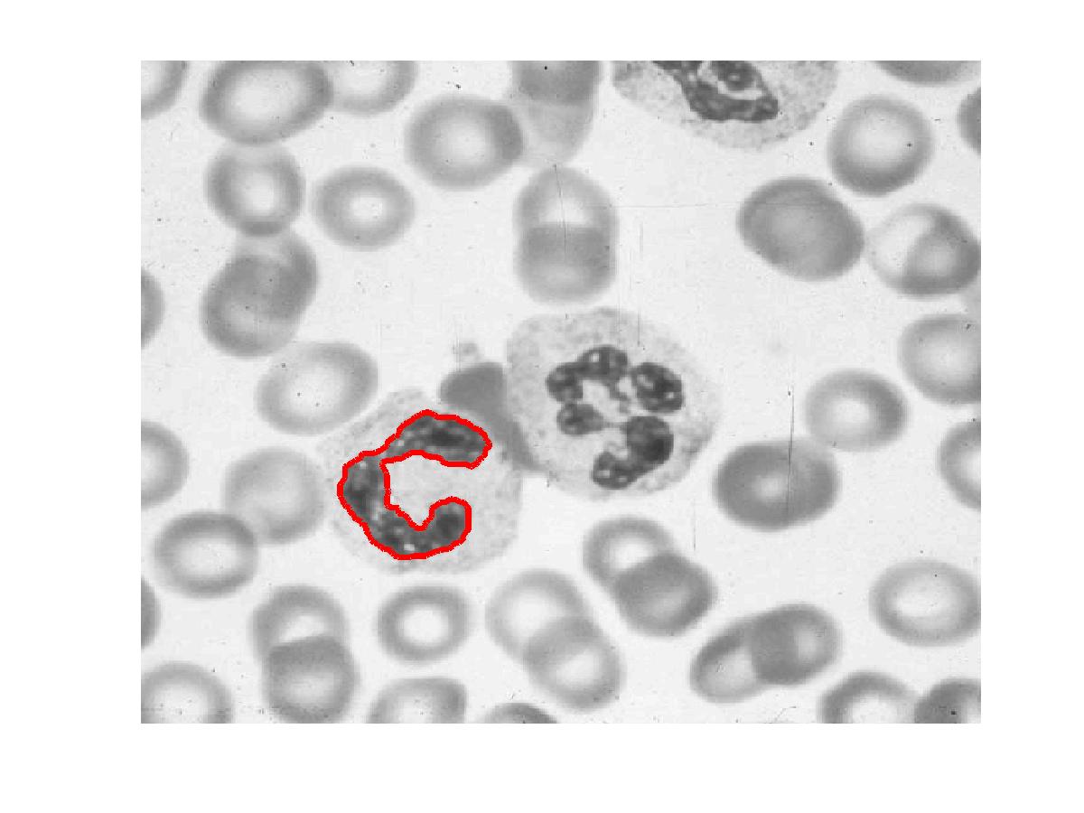
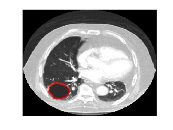
Figure 7: Algorithm 3 results; user selections and segmentation results.

5.3.   Complexity of Algorithm 3

We analyse Algorithm 3 to estimate the complexity of each multigrid cycle. We show analytically and experimentally that Algorithm 3 is $\mathcal{O}(N)$ as is expected for a multigrid method. We start with analysis of the complexity of the smoother, restriction operator, interpolation operator and coarse grid solver and then use the actual CPU times in Table 6 to confirm the predicted complexity.

Analytical complexity. Consider first only the fine grid with $N=nm$ pixels. Hybrid smoother 2 uses GSLEX-I on $K$ pixels and partial line smoothers on $L$ segments, containing the remaining $N-K$ pixels. GSLEX-I requires 13K operations. The partial line smoothers require $\mathcal{O}(M_{i})$ operation, where $M_{i}$ is the size of the line segment for $i\in[0,L]$. Suppose the number of operations for each partial line smoothing is $\kappa M_{i}$. We can therefore bound the complexity of the smoothing as $13K+\kappa\sum_{i=0}^{L}M_{i}$. We know that $K\leq N$ and we perform $4$ grid sweeps for every $\nu_{1}$ pre-smoothing steps and $\nu_{2}$ post-smoothing steps. For simplicity, assume a square image (i.e. $n=m$) and so for smoothing on one level we have

$$4(\nu_{1}+\nu_{2})\left(13K+\kappa\sum_{i=0}^{L}M_{i}\right)\leq 4(\nu_{1}+\nu_{2})(13N+\kappa nL)\leq 4(\nu_{1}+\nu_{2})(13+\kappa)N$$

operations. With a $V$- cycle over $T$ grids, the number of operations is

$$4(\nu_{1}+\nu_{2})(13+\kappa)N(1+\frac{1}{4}+\frac{1}{16}+\cdots+\frac{1}{2^{2(T-1)}})<4(13+\kappa)N\frac{\nu_{1}+\nu_{2}}{1-2^{-2}}=\frac{16(13+\kappa)(\nu_{1}+\nu_{2})}{3}N$$

The restriction operator has complexity at most $15N$ on the finest grid and with $M$ grids there are $M-1$ restrictions, hence a complexity of less than $20N$. Interpolation has complexity at most $5N$ on the finest grid and hence all interpolation operators contribute at most $\frac{20}{3}N$ operations. Finally, with AOS as the coarse grid solver each iteration needs $448N\cdot 2^{-2(M-1)}$ operations, this is clearly bounded by $448N$. Therefore the overall maximum complexity of Algorithm $3$ is

$$\frac{16(13+\kappa)(\nu_{1}+\nu_{2})}{3}N+20N+\frac{20}{3}N+448\nu_{AOS}N\leq\left[\frac{16(13+\kappa)(\nu_{1}+\nu_{2})}{3}+448\nu_{AOS}\right]N,$$

with $\nu_{AOS}$ the number of AOS iterations performed - as desired, the algorithm is $\mathcal{O}(N)$.

Experimental complexity. In Table 6 we show the ratio of the CPU times for Algorithm 3 on $\Omega^{h}$ when compared with the time on $\Omega^{2h}$. We see that the ratio is around 4 which linearly follows the increase in pixel number. Hence we see experimental confirmation of our analytical result that Algorithm 3 is an $\mathcal{O}(N)$ method.

6.   Conclusions

Image segmentation models provide a set of challenging and non-linear PDEs with non-smooth coefficients. Direct application of multigrid solvers with standard smoothers such as the lexicographic and line Gauss-Seidel smoothers leads to poor or no convergence. This paper has investigated the reasons why smoothers become ineffective due to non-smoothness of coefficients and proposed two hybrid smoothers that are aware of jumps and add extra local smoothing using non-standard iterative schemes. We find that both smoothers lead to convergent multigrid algorithms, however we recommend one smoother above the other as results are best experimentally and are shown to be good theoretically. Experiments confirm that the proposed new algorithm, outperforms the current fast methods. It also has optimal complexity and therefore is suitable for solving selective segmentation models for large images. Moreover, the ideas used in the design of the new smoother can be applied to other segmentation models and potentially non-smooth PDEs from other applications.

References

- [1] Rolf Adams and Leanne Bischof. Seeded region growing. IEEE Transactions on Pattern Analysis and Machine Intelligence, 16(6):641–647, 1994.
- [2] Raymond E. Alcouffe, Achi Brandt, Joel E. Dendy Jr., and J. W. Painter. The multi-grid method for the diffusion equation with strongly discontinuous coefficients. SIAM Journal on Scientific and Statistical Computing, 2(4):430–454, 1981.
- [3] N. Badshah and Ke Chen. Multigrid Method for the Chan-Vese Model in Variational Segmentation. Communications in Computational Physics, 4(2):294–316, 2008.
- [4] N. Badshah and Ke Chen. On two multigrid algorithms for modeling variational multiphase image segmentation. IEEE Transactions on Image Processing, 18(5):1097–1106, 2009.
- [5] N. Badshah and Ke Chen. Image selective segmentation under geometrical constraints using an active contour approach. Communications in Computational Physics, 7(4):759–778, 2010.
- [6] N. Badshah, Ke Chen, H. Ali, and G. Murtaza. A coefficient of variation based image selective segmentation model using active contours. East Asian J. Appl. Math., 2:150–169, 2012.
- [7] Egil Bae and Xue-Cheng Tai. Energy Minimization Methods in Computer Vision and Pattern Recognition, Lecture Notes in Computer Science 5681, chapter Efficient Global Minimization for the Multiphase Chan-Vese Model of Image Segmentationm, pages 28–41. Springer Berlin Heidelberg, Berlin, Heidelberg, 2009.
- [8] D Bai and Achi Brandt. Local mesh refinement multilevel techniques. SIAM Journal on Scientific and Statistical Computing, 8(2):109–134, 1987.
- [9] Achi Brandt. Multi-Level Adaptive Solutions to Boundary-Value Problems. Mathematics of Computation, 31(138):333–390, 1977.
- [10] Achi Brandt and Oren E. Livne. Multigrid techniques: 1984 guide with applications to fluid dynamics, volume 67. SIAM, 2011.
- [11] Carlos Brito-Loeza and Ke Chen. Multigrid algorithm for high order denoising. SIAM Journal on Imaging Sciences, 3(3):363–389, 2010.
- [12] Vicent Caselles, Ron Kimmel, and Guillermo Sapiro. Geodesic Active Contours. International Journal of Computer Vision, 22(1):61–79, 1997.
- [13] Tony F. Chan, Ke Chen, and Xue-Cheng Tai. Image Processing Based on Partial Differential Equations: Proceedings of the International Conference on PDE-Based Image Processing and Related Inverse Problems, CMA, Oslo, August 8–12, 2005, chapter Nonlinear Multilevel Schemes for Solving the Total Variation Image Minimization Problem, pages 265–288. Springer Berlin Heidelberg, Berlin, Heidelberg, 2007.
- [14] Tony F. Chan, Selim Esedoglu, and Mila Nikolova. Algorithms for Finding Global Minimizers of Image Segmentation and Denoising Models. SIAM Journal on Applied Mathematics, 66(5):1632–1648, 2006.
- [15] Tony F. Chan and Luminita A. Vese. Active contours without edges. IEEE Transactions on Image Processing, 10(2):266–277, 2001.
- [16] Ke Chen. Matrix Preconditioning Techniques and Applications. Cambridge University Press, 2005.
- [17] Ke Chen, Yiqiu Dong, and Michael Hintermüller. A nonlinear multigrid solver with line gauss-seidel-semismooth-newton smoother for the fenchel pre-dual in total variation based image restoration. Inverse Problems and Imaging, 5(2):323–339, 2011.
- [18] Gene H. Golub and Charles F. Van Loan. Matrix computations, volume 3. JHU Press, 2012.
- [19] Christian Gout, Carole Le Guyader, and Luminita A. Vese. Segmentation under geometrical conditions using geodesic active contours and interpolation using level set methods. Numerical Algorithms, 39(1-3):155–173, 2005.
- [20] Van E. Henson. Multigrid methods nonlinear problems: an overview. In Computational Imaging, volume 5016, pages 36–48, 2003.
- [21] Michael Kass, Andrew Witkin, and Demetri Terzopoulos. Snakes: Active contour models. International Journal of Computer Vision, 1(4):321–331, 1988.
- [22] M. Klodt, F. Steinbrücker, and Daniel Cremers. Moment Constraints in Convex Optimization for Segmentation and Tracking. Advanced Topics in Computer Vision, pages 1–29, 2013.
- [23] Carole Le Guyader and Christian Gout. Geodesic active contour under geometrical conditions: Theory and 3D applications. Numerical Algorithms, 48(1-3):105–133, 2008.
- [24] Xue-lei Lin, Xin Lu, Micheal K Ng, and Hai-Wei Sun. A fast accurate approximation method with multigrid solver for two-dimensional fractional sub-diffusion equation. Journal of Computational Physics, 323:204–218, 2016.
- [25] Fang Lu, Fa Wu, Peijun Hu, Zhiyi Peng, and Dexing Kong. Automatic 3D liver location and segmentation via convolutional neural networks and graph cut. arXiv preprint arXiv:1605.03012, 2016.
- [26] D. Mumford and J. Shah. Optimal approximation of piecewise smooth functions ans associated variational problems. Commu. Pure and Applied Mathematics, 42:577–685, 1989.
- [27] Artem Napov and Yvan Notay. Smoothing factor, order of prolongation and actual multigrid convergence. Numerische Mathematik, 118(3):457–483, 2011.
- [28] Thi Nhat Anh Nguyen, Jianfei Cai, Juyong Zhang, and Jianmin Zheng. Robust interactive image segmentation using convex active contours. IEEE transactions on image processing : a publication of the IEEE Signal Processing Society, 21(8):3734–43, 2012.
- [29] S. Osher and J. Sethian. Fronts propagating with curvature-dependent speed: algorithms based on Hamilton-Jacobi formulations. Journal of Computational Physics, 79(1):12–49, 1988.
- [30] Lavdie Rada and Ke Chen. A new variational model with dual level set functions for selective segmentation. Communications in Computational Physics, 12(1):261–283, 2012.
- [31] Lavdie Rada and Ke Chen. Improved Selective Segmentation Model Using One Level-Set. Journal of Algorithms & Computational Technology, 7(4):509–540, 2013.
- [32] Carmen Rodrigo, Francisco J Gaspar, and Francisco J Lisbona. On a local fourier analysis for overlapping block smoothers on triangular grids. Applied Numerical Mathematics, 105:96–111, 2016.
- [33] Jack Spencer and Ke Chen. A Convex and Selective Variational Model for Image Segmentation. Communications in Mathematical Sciences, 13(6):1453–1472, 2015.
- [34] U. Trottenberg, C. W. Oosterlee, and A. Schüller. Multigrid. Academic Press, 2001.
- [35] S Pratap Vanka. Block-implicit multigrid solution of navier-stokes equations in primitive variables. Journal of Computational Physics, 65(1):138–158, 1986.
- [36] L. A. Vese and T. F. Chan. A multiphase level set framework for image segmentation using the MS model. International Journal of Computer Vision, 50(3):271–293, 2002.
- [37] L. Vincent and P. Soille. Watersheds in digital spaces: an efficient algorithm based on immersion simulations. IEEE Trans. Pattern Analysis Machine Intell., 13(6):583–598, 1991.
- [38] W. L. Wan and T. F. Chan. Robust multigrid methods for nonsmooth coefficient elliptic linear systems. Journal of Computational and Applied Mathematics, pages 323–352, 2000.
- [39] J. P. Zhang, Ke Chen, and B. Yu. A 3D multi-grid algorithm for the CV model of variational image segmentation. International Journal of Computer Mathematics, 89(2):160–189, 2012.
- [40] Yunrong Zhu. Analysis of a multigrid preconditioner for Crouzeix-Raviart discretization of elliptic partial differential equation with jump coefficients. Numerical Linear Algebra with Applications, 21(1):24–38, 2014.