Hollowness Effect and Entropy in High Energy Elastic Scattering

Abstract

This paper presents a qualitative explanation for the hollowness effect based on the inelastic overlap function, claiming this result is a consequence of fundamental thermodynamic processes. Using the Tsallis entropy, one identifies the entropic index $w$ with the ratio of the collision energy to critical one in the total cross-section. The integrated probability density function is replaced by the inelastic overlap function, which represents the probability of occurrence of an inelastic event depending on both the collision energy and impact parameter. The Coulomb potential, as well as the confinement potential, are used as naive approaches to describe the (internal) energy of the colliding hadrons. The Coulomb potential in the impact parameter picture is not able to furnish any reliable physical result near the forward direction. However, the confinement potential in the impact parameter space results in the hollowness effect shown by the inelastic overlap function near the forward direction.

I Introduction

The proton-proton ($pp$) and antiproton-proton ($\bar{p}p$) elastic scattering at high energies remain as one of the most surprising open issues of the collision processes. Some of these open questions may be solved by the new phase of the so-called High Luminosity Large Hadron Collider (HL–LHC), which will deliver 3 ab^-1 of integrated luminosity CERN-YR-2019-007 . In the future, other issues certainly will arise, resulting in the construction of novel models or the improvement of the present-day ones.

As well-known, the geometric point of view of $pp$ and $\bar{p}p$ scattering is an important tool to describe its dynamics, furnishing insights as well as approaches for the non-perturbative QCD. Of course, (anti)protons are not point-like objects, but in wide energy range, they behave similar to the black disk picture anisovich_nikonov ; V.V.Anisovich.M.A.Matveev.V.A.Nikonov.Int.J.Mod.Phys.A31.1645019.2016 of classical optics, as can be observed in the experimental results obtained over last decades sdcvaocvm . Correspondence to the black disk means a large probability of absorption (approaches to unity, strictly speaking) for some range of the quantity used in a certain model. Usually, that quantity is the impact parameter $b$. It should be clarified that the above statement, concerning the behavior of the (anti)protons, describes only a qualitative approach to the black disk regime at an accuracy level $\sim 10\%$ for values $b\to 0$. In general, it believes that hadrons slowly turns into BEL (Blacker – Edger – Larger) with the increase of $s$ Cheng-book-1987 ; Barone-book-2002 . However, some recent experimental results and model approaches, briefly discussed below, indicate this picture is not accurate enough. Thus, the situation is quite complicated as well as far from an unambiguous physical conclusion. The new experimental and phenomenological studies will be crucially important for a deeper understanding of the geometry of the interaction region concerning the hadronic, in particular, $pp$, $\bar{p}p$ collisions.

From the original hypothesis pointed out in dremin_1 ; dremin_2 and later in broniowski_arriola , the gray area, also known as hollowness effect, suggests that at very high energies the inelastic profile function at zero impact parameter does not reach the unit. This unexpected behavior was subject of a series of explanations broniowski_arriola ; alkin_martynov ; anisovich_nikonov ; dremin_1 ; troshin_tyurin_1 ; anisovich ; troshin_tyurin_2 ; albacete_sotoontoso ; arriola_broniowski ; dremin_2 . However, none of these approaches took into account the entropy of the internal constituents of the hadron and associated with the elastic scattering in the impact parameter space. As shown in sdcvaocvm , the Tsallis entropy (TE) can be connected with the inelastic overlap function and with the squared critical energy $s_{c}$, associated with a phase transition in the internal structure of (anti)proton which manifests itself via the total cross section dataset. This phase transition is of topological order, just like the BKT phase transition occurring in the XY–model sdcvaocvm . In this kind of phase transition, there is no spontaneous symmetry breaking but only a rearrangement of the internal constituents to some more favorable geometry configuration. This critical value divides the total cross section experimental data into two samples with different fractal dimensions, exposing the presence of a multifractal character in this physical quantity bc . It is important to stress here that the TE emerges exactly in the context of multifractal structures tsallis_multifractal .

On the other hand, the multifractal feature also occurs in the momentum space antoniou_1 ; antoniou_2 ; antoniou_4 ; antoniou_5 ; bialas_1 ; bialas_2 , reinforcing the necessity of using the TE, as shown in deppman_phys_rev_d93_054001_2016 . Thus, the multifractality of $pp$ and $\bar{p}p$, in different variables, should be noted in the impact parameter space, revealing some novel physical aspect, for example, in the behavior of the inelastic overlap function.

To the complete development of the present approach, one needs the calculation of the internal energy of the hadron. However, this is a very hard, and presently, an unsolved question. Thus, at first glance, one proposes the study of two non-relativistic potentials mimicking the (internal) energy of the hadron in the impact parameter space. The first one is the Coulomb potential being used to represent the total energy of the hadron, which results in the $pp$ and $\bar{p}p$ elastic scattering as billiard ball collisions. Of course, this potential is unable to present results about the internal structure of the hadrons supposed structureless in this case. The approximations performed prevents the extraction of any information near the forward direction ($b<b_{\scriptsize{\mbox{min}}}$). The second approach uses the confinement potential and, contrary to the first one, it allows the presence of an internal structure due to the quarks and gluons. The consequence of the confinement potential, in this case, we claim here, is the arising of the hollowness effect near the forward direction, as shall be seen in this work.

It is important to stress that, in the present thermodynamic approach, we are not interested in presenting a model that produces the best fittings result of the experimental data. The interest here is to study the physical consequences of a phase transition occurring in the $pp$ and $\bar{p}p$ elastic scattering from the TE in the impact parameter space.

The paper is organized as follows. In section II one sets the problem, and a brief review is presented for the experimental situation with absorption in the $pp$ and $\bar{p}p$ collisions. Section III is devoted to general statements, and formalism is introduced, allowing interrelations between thermodynamic quantities, in particular, the internal energy, and the effective potentials in some quantum field theories. In section IV the Coulomb potential is considered. The possible manifestation of the hollowness effect in the strong interaction, in particular, in $pp$ and $\bar{p}p$ collisions is presented in section V with help of the confinement potential. Finally, section VI contains the discussions and conclusions.

II Hollowness Effect and Entropy

The high energy $pp$ and $\bar{p}p$ elastic scattering can be analyzed using both the transferred momentum $q^{2}$ or the impact parameter $b$ since these variables can be connected through a Fourier–Bessel transform. Thus, the physical constraints of one space can be rewritten in another one, sometimes revealing details or furnishing insights to solve a problem.

II.1 Inelastic overlap function

The impact parameter space is the geometric scenario of the elastic scattering, possessing clear classical appeal. In this sense, it is natural to use the black disk picture to describe the $pp$ and $\bar{p}p$ elastic scattering at high energies. The elastic scattering amplitude $F(s,q^{2})$ is written using the impact parameter $b$ as

$$F(s,q^{2})=i4\pi{\int_{0}}^{\infty}bdbJ_{0}(qb)\bigl{\{}1-\exp[i{\chi}(s,b)]\bigr{\}}=i4\pi{\int_{0}}^{\infty}bdbJ_{0}(qb)\mathrm{\Gamma}(s,b),$$ (1)

and here $\sqrt{s}$ is the collision energy in the center-of-mass system, $J_{0}(x)$ is a zeroth order Bessel function, and $\chi(s,b)$ is the eikonal function written as

$$\chi(s,b)=\mathrm{Re}\chi(s,b)+i\mathrm{Im}\chi(s,b),~{}~{}~{}\mathrm{Im}\chi(s,b)\geq 0,$$ (2)

where the imaginary part corresponds to the opacity function, identified with the matter distribution inside the incident particles. It is used the following view of the optical theorem $s^{-1}\mathrm{Im}F(s,0)=\sigma_{\scriptsize{\mbox{tot}}}(s)$, where $\sigma_{\scriptsize{\mbox{tot}}}(s)$ is the total cross section for the interaction process sdcvaocvm .

The profile function $\Gamma(s,b)=\mathrm{Re}\Gamma(s,b)+i\mathrm{Im}\Gamma(s,b)$ is the elastic scattering amplitude in the impact parameter space for $s$ fixed, being able to give an estimate of the particle interacting radius as well as an glance of its internal structure. Furthermore, the unitarity condition can be written using the inelastic overlap function as

$$0\leq G_{\scriptsize{\mbox{inel}}}(s,b)=2\mathrm{Re}\Gamma(s,b)-|\Gamma(s,b)|^{2}\leq 1,$$ (3)

that represents the absorption probability of a given $(s,b)$ and, one expects that moving away from the forward collision $(b=0)$, the interaction probability diminishes. The general belief is that, at $b=0$ and for a sufficient high energy, $G_{\scriptsize{\mbox{inel}}}(s,0)\to 1$. This result implies that for $s\to\infty$ the $pp$ and $\bar{p}p$ elastic scattering tends to present the same physical behavior in the forward direction. This behavior is expected to occur due to the leading pomeron exchange S.D.Campos.Phys.Scr.95.065302.2020 ; S.D.Campos.arXiv.2003.11493.2020 .

Several theorems were proven from the 1960s, and some of them established the fundamental theoretical basis of the high-energy elastic scattering. For instance, the elastic to total cross section ratio is one of these remarkable results obtained from a well-established basis froissart_1961 ; lukaszuk_1967 ; martin_2009 ; wu_2011 ; PRD-91-076006-2015 . The detailed analysis of this cross section ratio in nucleon-nucleon collisions arXiv-1805.10514 shows that, at high energies, the approximate relation

$$\sigma_{\scriptsize{\mbox{el}}}(s)/\sigma_{\scriptsize{\mbox{tot}}}(s)\approx 1/4$$ (4)

holds for $pp$ up to the highest experimentally reached energy $\sqrt{s}=57$ TeV within the error bars for this experimental data. Based on the measured $\sigma_{\scriptsize{\mbox{el}}}(s)/\sigma_{\scriptsize{\mbox{tot}}}(s)$ the quantity $G_{\scriptsize{\mbox{inel}}}(s,0)$ was estimated in unprecedented wide energy range sdcvaocvm . These estimations agree reasonably with the model-dependent results obtained some earlier NPB-166-301-1980 ; PLB-132-443-1983 ; PLB-160-167-1985 , but the accuracy of the method from sdcvaocvm is usually worse than that for the approach based on the parameterization of the scattering amplitude NPB-166-301-1980 . The accuracy is $\sim 10\%$ for the method from sdcvaocvm and does not allow rigorous and unambiguous conclusions. On the other hand, within the last approach, the evolution of $G_{\scriptsize{\mbox{inel}}}(s,0)$ on $s$ can be studied considering whole experimental energy range available, as commented above. It seems to be an important advantage for the method from sdcvaocvm . The intermediate-energy estimations for $G_{\scriptsize{\mbox{inel}}}(s,0)$ in nucleon-nucleon scattering can be approximated by assuming $G_{\scriptsize{\mbox{inel}}}(s,0)\sim 0.9$ constant and some growth is only obtained for $\sqrt{s}>100$ GeV. As seen, the probability of absorption is close to unity within accuracy $\sim 10\%$ for central collisions at intermediate energies already. The constant behavior of $G_{\scriptsize{\mbox{inel}}}(s,0)$ agrees quite well with the results for the Intersecting Storage Rings (ISR) energy range NPB-166-301-1980 . The noticeable increase $s$ from the $\sqrt{s}=52.8$ GeV for $pp$ up to the $\sqrt{s}=546$ GeV for $\bar{p}p$ leads to the corresponding growth of the inelastic overlap function in central collisions from $G_{\scriptsize{\mbox{inel}}}(s,0)\approx 0.9264$ PLB-132-443-1983 up to the $G_{\scriptsize{\mbox{inel}}}(s,0)\approx 0.9764$ for $\bar{p}p$ interactions PLB-160-167-1985 indicating the slight growth of the probability of absorption. The increase is confirmed based on a significantly richer experimental material discuted elsewhere sdcvaocvm , and it provides a constant $G_{\scriptsize{\mbox{inel}}}(s,0)\sim 1.0$ starting with $\sqrt{s}=546$ GeV up to the highest experimentally reached energy $\sqrt{s}=57$ TeV. In fact results from sdcvaocvm confirm the general statement made in Sec. I that the (anti)proton turns blacker with the increase of $s$. This statement agrees with the estimations of $G_{\scriptsize{\mbox{inel}}}(s,0)$ for $pp$ collisions at $\sqrt{s}=7$ TeV PRD-89-051901-2014 indicated by the reaching of the black disk limit and obtained within the modified method from NPB-166-301-1980 . The black spot appears at the LHC energies $\sqrt{s}\sim 10$ TeV in the central region for both the mode of the (black) partonic disk and the mode of the resonating partonic disk anisovich . On the other hand, the mass squared approach with central optical potential shows a shallow minimum at $b=0$ with depth of few percents of the maximum $G^{\scriptsize{\mbox{max}}}_{\scriptsize{\mbox{inel}}}(s,b)=1$, whereas the maximum shifts to $b>0$ at the LHC energies $\sqrt{s}=7$ and 14 TeV arriola_broniowski . This result is corroborated by the observation of a hollowness, i.e. a shallow minimum with depth $\sim 1\%$ of the maximum at $\sqrt{s}=13$ TeV within the dipole Regge model PRD-98-074012-2018 and the Lévy imaging T.Csorgo.R.Pasechnik.A.Ster.Euro.Phys.J.C80.126.2020 . In the last case, the analysis of the high statistic data at $\sqrt{s}=13$ TeV EPJC-79-861-2019 allows the observation of the proton hollowness effect with beyond 5 s.d. (standard deviation) significance. The analytic extrapolation for $G_{\scriptsize{\mbox{inel}}}(s,0)$ calculated for an ultra-high energy range in sdcvaocvm predicts the onset of deviation from the black disk limit at $\mathcal{O}$(100 TeV), and the continuing decreasing of the inelastic overlap function in central nucleon-nucleon collisions with the growth of $s$ provides $G_{\scriptsize{\mbox{inel}}}(s,0)\to 0$ for PeV energies. In particular, the PeV energy domain is considered as the low boundary for the collision energy for the onset of the noticeable difference between two modes of the partonic disk, black and resonating ones anisovich . One can note that the toroid shape of the inelastic interaction region is also evaluated within the assumption that $\mathrm{Im}\,F(s,q^{2})>0$ everywhere, with deviation of $G_{\scriptsize{\mbox{inel}}}(0)$ from unit at level of few percentages for multi-TeV energy domain $\sqrt{s}\gtrsim 10$ TeV EPJC-78-913-2018 . Thus, this brief review confirms the current complex and ambiguous situation in theoretical and experimental studies about the geometry of the hadronic collisions, mostly for $pp$ and $\bar{p}p$.

The unitarity equation (3) also can be written as

$$G_{\scriptsize{\mbox{inel}}}(s,b)=\mathrm{Re}\Gamma(s,b)[2-\mathrm{Re}\Gamma(s,b)]-\mathrm{Im}^{2}\Gamma(s,b).$$ (5)

That result can be rewritten taking into account derivative dispersion relations as well as the crossing property to $\mathrm{Im}\Gamma(s,b)$. Notice that derivative contributions depend on the transferred momentum range. Thus, for $q^{2}\to 0$, the derivative contribution occurs in the periphery, while for $q^{2}\to\infty$, the contribution is central. Then, the expression (5) possess two regimes, depending on $b$ is central or peripheral. Considering large values of $b$, $\mathrm{Im}\Gamma(s,b)\approx\mathrm{Re}\Gamma(s,b)$ and, therefore, derivative terms should be taken into account. However, for small values of $b$, $\mathrm{Im}\Gamma(s,b)\ll\mathrm{Re}\Gamma(s,b)$, and derivative terms can be neglected. Considering only small values of $b$, one writes

$$G_{\scriptsize{\mbox{inel}}}(s,b)\approx\mathrm{Re}\Gamma(s,b)[2-\mathrm{Re}\Gamma(s,b)],$$ (6)

and one can identify $1\leq\mathrm{Re}\Gamma(s,b)\leq 2$, where $\mathrm{Re}\Gamma(s,b)=2$ is the completely non-absorptive case and $\mathrm{Re}\Gamma(s,b)=1$ is the full absorptive case. Taking the partial derivative with respect to $b$ of (6), one obtains ($\partial_{x}\equiv\partial/\partial x$)

$$\partial_{b}G_{\scriptsize{\mbox{inel}}}(s,b)\approx 2\partial_{b}\mathrm{Re}\Gamma(s,b)[1-\mathrm{Re}\Gamma(s,b)].$$ (7)

Note that at some critical value $b_{c}$, the $\left.\partial_{b}G_{\scriptsize{\mbox{inel}}}(s,b)\right|_{b=b_{c}}=0$ can be reached if $\left.\partial_{b}\mathrm{Re}\Gamma(s,b)\right|_{b=b_{c}}=0$ and / or $\mathrm{Re}\Gamma(s,b_{c})=1$. The $and$ connective means that $b_{c}$ is a critical value and the process is completely absorptive at $b_{c}$. On the other hand, the $or$ case is analyzed as follows. If $\left.\partial_{b}\mathrm{Re}\Gamma(s,b)\right|_{b=b_{c}}=0$ but not $\mathrm{Re}\Gamma(s,b_{c})=1$, then $b_{c}$ is a critical value not representing the full absorptive case, i.e. the inelastic overlap function does not produce the black disk pattern at $b_{c}$. On the contrary, the full absorptive case does not represent a critical point of $\mathrm{Re}\Gamma(s,b)$. This is the non-physical result since the inelastic overlap function is limited. Thus, there are two situations able to furnish a zero in $\partial_{b}G_{\scriptsize{\mbox{inel}}}(s,b)$ at some impact parameter critical value, $b=b_{c}$. The first situation can be achieved considering that at $b=b_{c}$ the $\left.\partial_{b}\mathrm{Re}\Gamma(s,b)\right|_{b=b_{c}}=0\bigcap\mathrm{Re}\Gamma(s,b_{c})=1$, hence $b_{c}$ is a critical value and represents the full absorptive case. The second situation can be achieved if $\left.\partial_{b}\mathrm{Re}\Gamma(s,b)\right|_{b=b_{c}}=0\bigcap\mathrm{Re}\Gamma(s,b_{c})\neq 1$.

Taking into account the allowable range for $\mathrm{Re}\Gamma(s,b)$, then the sign of $\partial_{b}\mathrm{Re}\Gamma(s,b)$ determines the sign of $\partial_{b}G_{\scriptsize{\mbox{inel}}}(s,b)$. Considering $\partial_{b}G_{\scriptsize{\mbox{inel}}}(s,b)>0$, the only possible physical result is $\partial_{b}\mathrm{Re}\Gamma(s,b)<0$ and vice versa. Then, the sign of $\partial_{b}G_{\scriptsize{\mbox{inel}}}(s,b)$ is controlled only by the sign of $\partial_{b}\mathrm{Re}\Gamma(s,b)$, and the inelastic overlap function change its sign in agreement with $b$ (fixed $s$). As stated above, $\mathrm{Re}\Gamma(s,b)$ is related to the imaginary part of $F(s,q^{2})$ and, changing the sign of $\mathrm{Im}F(s,q^{2})$, this also represents a changing in the sign of $\mathrm{Re}\Gamma(s,b)$. As well-known, $\mathrm{Im}F(s,q^{2})$ oscillate according to $q^{2}$ and, therefore, the sign change of $\partial_{q}\mathrm{Im}F(s,q^{2})$ occurs as $q^{2}$ grows.

II.2 The Tsallis entropy approach

On the other hand, one can analyze the behavior of $G_{\scriptsize{\mbox{inel}}}(s,b)$ considering the TE. Notice that exists several ways to compute the entropy of a thermodynamic system, being the well-known Boltzmann entropy the most popular. This entropy is applied, usually, into a system of non-interacting particles. Hence, this entropy is additive: the entropy of the whole system is the sum of each subsystems entropy. However, a system containing interacting subsystems (sometimes strongly correlated) needs an entropy calculation that takes this feature into account.

The TE can naturally be applied into correlated systems since it is non-additive. Moreover, Rényi entropy renyi_entropy , Shannon entropy shannon_entropy , Abe entropy abe_entropy and Boltzmann entropy, for instance, can be reduced to the TE beck_0902.1235v2 ; tsallis_book . Furthermore, the TE possesses two (among others) interesting mathematical properties: it is concave for all $w>0$, a crucial characteristic for an entropy function. Besides, it also obeys the Lesche stability condition, i.e. it is stable under small perturbations of probabilities. Considering these properties, the TE is able to furnish a description of the physical system under study.

Bearing in mind the above considerations the TE entropic index $w$ can be replaced by the ratio sdcvaocvm

$$w=s/s_{c},$$ (8)

where $s_{c}$ is the squared critical energy associated with the BKT-like phase transition sdcvaocvm , whose consequence is the fractal structure of the total cross-section bc . In this sense, $w$ plays the physical role of a transition parameter. When $s>s_{c}$, the fractal dimension is positive and negative when $s<s_{c}$, i.e. the TE possess two behaviors depending on $w>1$ or $w<1$. On the other hand, the negative fractal dimension can be viewed as a measure of the hadron emptiness (the slowdown part of the total cross-section data set); the positive fractal dimension can be associated with the usual measure of the total cross section (the growing part of the total cross-section data) bc .

In sdcvaocvm , the TE is identified with the scattering at fixed $s$ by means of the inelastic overlap function $G_{\scriptsize{\mbox{inel}}}(s,b)$, due to non-elastic $s$-channel intermediate states as ($k\equiv s/s_{c}-1$)

$$S_{T}\equiv S_{T}(s,b)=k^{-1}[1-G_{\scriptsize{\mbox{inel}}}(s,b)],$$ (9)

where the probability of an event in the impact parameter space $\displaystyle P(s,b)=\int_{0}^{b}\bigl{[}p\,(b^{\prime})\bigr{]}^{s/s_{c}}db^{\prime}$ is replaced by $G_{\scriptsize{\mbox{inel}}}(s,b)$ within the hypothesis for using of the TE in the $b$-space and, for the sake of simplicity, one assumes $m=1$ and $n=1$ sdcvaocvm . It is interesting to note that unitarity demands $0\leq G_{\scriptsize{\mbox{inel}}}(s,b)=1-kS_{T}\leq 1$ implying the replacement $kS_{T}\rightarrow\tilde{S}_{T}$, where $\tilde{S}_{T}\equiv kS_{T}$ is the normalized entropy.

As well-known, the inelastic overlap function takes into account all intermediate inelastic channel contributions. Thus, the entropy (9) can be associated with the inelastic scattering contributions. In the above result, if $G_{\scriptsize{\mbox{inel}}}(s,b)\to 1$ (the black disk limit) then $S_{T}\to 0$. The physical meaning of this result is simple: at the black disk limit, the system (the motion of the internal constituents) is in its lowest (or highest) possible value, as stated by Quantum Mechanics. Therefore, the physical state of the system is well defined.

The inelastic overlap function is interpreted as the probability of an inelastic scattering in a given $(s,b)$. Thus, $G_{\scriptsize{\mbox{inel}}}(s,b)=1$ implies that at head-on collision $b=0$ (or at some $b\neq 0$ as professed by the hollowness effect), the probability achieves its maximum as well as the entropy tends to its minimum. The general belief is that when $s\to\infty$ the black disk limit is achieved at $b=0$. However, this is not necessarily true since there is a sign change in the TE in accordance with $s/s_{c}$. To see this, observe that partial derivative of $S_{T}$ with respect to $b$ is given by

$$\partial_{b}S_{T}(s,b)=-k^{-1}\partial_{b}G_{\scriptsize{\mbox{inel}}}(s,b).$$ (10)

Assuming $s>s_{c}$ (high energies regime), the sign of $\partial_{b}S_{T}$ is determined by the sign of $\partial_{b}G_{\scriptsize{\mbox{inel}}}(s,b)$. In this regime, the fractal dimension of the total cross section is positive representing the matter density increase inside the hadron bc . Therefore, in accordance with the above analysis, $b_{c}$ determines the region inside the hadron where the entropy increases ($b>b_{c}$) or decreases ($b<b_{c}$). On the other hand, considering $s<s_{c}$ (low energies regime), the existence of $b_{c}$ implies in an increasing ($b<b_{c}$) or decreasing ($b>b_{c}$) entropy. The fractal dimension of the total cross section is negative, representing the emptiness or the absence of a well-defined internal structure inside the hadron bc . The same result can be obtained replacing (7) into (10), showing a matter distribution in accordance with the existence of $b_{c}$ and determining the entropy behavior.

III Internal Energy and Effective Potential

Assuming statistical equilibrium between a heat reservoir with the temperature $\Theta$ and a hadron the later can be considered as the canonical ensemble of its constituents at temperature $T$ and consequently for nonextensive statistics PA-261-534-1998

$$\partial_{\mathcal{U}}\tilde{S}_{T}=\tilde{T}^{-1},$$ (11)

where definition of the canonical ensemble Levich-book-1971 ; JIKapusta-GCharles-book-2006 or, equivalently, closed system kaufman_book_2001 is taken into account, $\mathcal{U}$ is the hadron internal energy, $\tilde{T}\equiv T/k$ is the normalized temperature of the constituent ensemble under consideration, $\Theta=T$ Levich-book-1971 and $T=T(s,b)$ due to corresponding dependences of ${S}_{T}$.

In consonance with the preceding section, $S_{T}$ is replaced by its normalized form since $G_{\scriptsize{\mbox{inel}}}(s,b)$ obey the unitarity condition. Therefore, the entropy of the above system of constituents also can be written using the thermodynamics. The approach of the canonical ensemble or, more generally, grand canonical one at negligibly small chemical potential, allows the suggestion a constant Helmholtz free energy ($\mathcal{F}$). Therefore the (11) can be rewritten in the standard integral form $\mathcal{U}=\mathcal{F}+\tilde{T}\tilde{S}_{T}$ in which the constant of integration is assigned as $\mathcal{F}$. The quantity $\mathcal{U}$, as well-known, cannot be deduced from the first principles of thermodynamics. For quantum systems studied here $\mathcal{U}$ can be reduced to the potential energy $E_{p}$ Shuryak-book-2004-p374 which is a function of the effective potential $V$, thus $\mathcal{U}\approx E_{p}(V)$. Of course, this rough approximation excludes the kinetic term and the action due to external forces. Taking into account $V(s,r)=E_{p}(s,r)-E_{p}(s,\infty)$ PRD-70-054507-2004 one can derive $V+E_{p}(s,\infty)\approx\mathcal{F}+\tilde{T}\tilde{S}_{T}$, where $r$ is the distance between constituents. For an Abelian quantum field theory (QFT), like QED, $E_{p}(s,\infty)=0$. The hadron as a statistical system will spontaneously undergo a process if it lowers the systems Helmholtz free energy kaufman_book_2001 . Thus the ordinary hadron should be characterized by the lowest value of $\mathcal{F}$ which can be assigned as the zero (ground) level. On the other hand, in some non-Abelian QFT, like QCD in the pure gauge limit, $E_{p}(s,r\to\infty)\to\infty$ and the Helmholtz free energy tends to the infinitely large value at $r\to\infty$ within the approach of a static constituents at temperature smaller than $T$ of a phase transition. Such cold system can be considered as a stationary confinement state, i.e. as (quasi)hadron in the strong interaction field. Moreover similar growth can be suggested for $E_{p}$ and $\mathcal{F}$ at increasing of $r$ for any distances at negligibly small $T$ based on the available results for finite values of $r$ obtained with help of the lattice QCD calculations AIPCP-602-323-2001 ; PTPSuppl-153-287-2004 as well as the phenomenological studies, in particular, within $T$-matrix formalism NPA-941-179-2015 . Therefore assuming a mutual reduction of the terms $E_{p}(s,\infty)$ and $\mathcal{F}$, at least, qualitatively as well as an appropriate replacement $r\to b$ the following general relation can be deduced for a stationary state

$$V(s,b)\approx\tilde{S}_{T}(s,b)\tilde{T}(s,b),$$ (12)

It should be stressed that the Bohm’s quantum potential can be used to mimic the internal energy of a quantum system, giving insight into its role in stationary states G.Dennis.M.A.de.Gosson.B.J.Hiley.Phys.Lett.A378.2363.2014 . Then, in the Bohm’s point of view, the particle is not a point-like object, contrariwise, it possesses an internal structure with some topological geometry. As shall be seen, this extended structure is necessary to explain the hollowness effect.

The temperature must be normalized to obey the unitarity condition. On the other hand, the relevant information here is the sign of the temperature, depending on $s$, since this approach (the use of the effective potential) does not allows the precise knowledge of the critical temperature. Hence, normalizing the temperature one still maintain the relevant information about its sign only by using the procedure

$$\tilde{T}(s,b)=\left\{\begin{array}[]{lcl}\displaystyle+1,&\mbox{if}&s<s_{c}\\ \displaystyle-1,&\mbox{if}&s>s_{c}\\ \end{array}\right.$$ (15)

Mathematically speaking, the only requirement to obtain a negative temperature is that the entropy should not be restricted to monotonically increasing of $\mathcal{U}$ ramsey_phys_rev_103_10_1956 . Its physical meaning is also well-defined: the occupation distribution is inverted, where high-energies states are populated more than low-energies states. The occupation probability of a quantum state increases exactly with the energy of the state. Keeping the information about the phase transition, the qualitative behavior of the inelastic overlap function is studied here. Based on the (12) the following chain of the equations can be obtained within the potential approach: $\partial_{b}\tilde{S}_{T}=\tilde{T}^{-1}(s,b)\partial_{b}V(s,b)-V(s,b)\tilde{T}^{-2}(s,b)\partial_{b}\tilde{T}(s,b)=\tilde{T}^{-1}(s,b)\partial_{b}V(s,b)$ taking into account (15). Then, it is deduced the particular relation $\partial_{b}G_{\scriptsize{\mbox{inel}}}(s,b)=-\tilde{T}^{-1}(s,b)\partial_{b}V(s,b)$, in which one can use $|\tilde{T}(s,b)|$ without lost of generality. It allows the use of a simple ansatz

$$G_{\scriptsize{\mbox{inel}}}(s,b)=1-\tilde{V}(s,b),$$ (16)

to solve the last differential equation within the potential approach, where $\tilde{V}(s,b)$ can be obtained with the help of some procedure from the potential $V(s,b)$ in order to preserve the validity of the unitarity condition (3). Taking into account this condition, then $0\leq\tilde{V}(s,b)\leq 1$ and, consequently, the normalization can be suggested as such procedure with the specific details depending on the view and behavior of the $V(s,b)$ in the kinematic region under study. It should be noted that there are some restricted ranges for the impact parameter ($b_{\scriptsize{\mbox{min}}}\leq b\leq b_{\scriptsize{\mbox{max}}}$) and for the collision energy ($s_{\scriptsize{\mbox{min}}}\leq s\leq s_{\scriptsize{\mbox{max}}}$), since in hadronic interactions these parameters are characterized by finite values for the boundaries $b_{\scriptsize{\mbox{min}/\mbox{max}}}$, $s_{\scriptsize{\mbox{min}/\mbox{max}}}$ due to, in general, finite space scales (”sizes”) of incoming particles and finite collision energy for any physical process. The reliable values of the boundaries $b_{\scriptsize{\mbox{min}/\mbox{max}}}$, $s_{\scriptsize{\mbox{min}/\mbox{max}}}$ are defined within concrete approach used and /or kinematic features of the reaction under consideration. The following general statement can be obtained from (16): the black disk regime $G_{\scriptsize{\mbox{inel}}}(s,b)\to 1$ is reached only if $\tilde{V}(s,b)\to 0$ in some kinematic domain and / or separate points of the $(s,b)$ plane. Thus, within the potential approach, the above ansatz produce the result

$$\tilde{S}_{T}(s,b)=\tilde{V}(s,b)$$ (17)

replacing (16) into the relation (9). Consequently, the $b$-dependence of the TE is the same as for effective potential $\tilde{V}(s,b)$. In general, the $s$-dependence of the $S_{T}$ for certain types of the potential $V(s,b)$ can be deduced with the help of equation (17) and $k$, in agreement with the definition of normalized TE and the appropriate choice of $s_{c}$. In addition, one can note that the equation (17) is in accordance with (11) taking into account the replacement $\mathcal{U}\to V$ and normalization (15) made above.

Depending on the potential used, this assumption allows or not a view on the internal structure of the particles. One considers here two potentials in the impact parameter space as attempts to explain the behavior of the inelastic overlap function. The first one is the well-known Coulomb potential, which allows a naive view of the inelastic overlap function from the outside of the hadron. This potential is used for structureless particles. The second one is the confinement potential that represents the point of view of the constituents of the hadron sdcvaocvm . One supposes this thermodynamic system is described by the canonical ensemble, where particle exchange is forbidden. Thus, the proton, as well as the antiproton, is a composite particle, turning relevant know how the collision energy is shared among the quarks and gluons. That question is quite similar to the multiplicity scenario and will be discussed further.

IV Coulomb Potential

At this first moment, one assumes the Coulomb potential as being able to describe the hadron energy treating it as a point-like particle. Despite this naive approach, it can furnish at least a classical picture of the inelastic overlap function. Assuming $r=|\mathbf{r}_{i}-\mathbf{r}_{j}|$ as the distance between hadrons placed at $\mathbf{r}_{i}$ and $\mathbf{r}_{j}$ and with masses $m_{h}^{2}\ll s$, then using the impact parameter $b$ one can approximate the Coulomb potential $V_{\scriptsize{\mbox{C}}}(r)=-a/r$ at fixed $s$ by

$$V_{\scriptsize{\mbox{C}}}(r)\approx V_{\scriptsize{\mbox{C}}}(s,b)=-ab^{-3}\bigl{(}b^{2}-2/s\bigr{)}.$$ (18)

The above representation can be obtained by noting that $b=r\cos\theta$ is the projection of $r=|\vec{r}|$ onto $b=|\vec{b}|$, where $\theta$ is the angle between $\vec{b}$ and $\vec{r}$, where $r=|\vec{r}|$ is the distance between the hadrons. Moreover, $q^{2}=2k^{2}(1-\cos\theta)$ and $s/2-2m^{2}=2k^{2}$, where $m$ is hadron mass and $k=|\vec{k}|$ is the norm of the three-momentum Barone-book-2002 . The parameter $a>0$ is dimensionless corresponding to the electrostatic interaction of pair. Note the result (18) can be written as $V_{\scriptsize{\mbox{C}}}(s,b)\approx-ab^{-1}$ for a sufficient high fixed-$s$. Fig. 1 shows the $b$- (a) and the $s$-dependence (b) for exact view of Coulomb potential and its approximation in the impact parameter space (18). In the latter case, the curves are shown for fixed $\sqrt{s}=31.0$ and 52.8 GeV (Fig. 1a) and for fixed $b=0.01$ and 0.02 fm (Fig. 1b).

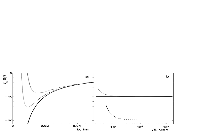
Figure 1: Dependence of the exact view of Coulomb potential (solid lines) and approximate relation (18) on the (a) impact parameter and (b) collision energy: a – the dotted line corresponds to the approximation (18) at $\sqrt{s}=31.0$ GeV and the dashed line – to the (18) at $\sqrt{s}=52.8$ GeV; b – the dotted curve is the approximation (18) at $b=0.02$ fm and the dashed line – the (18) with $b=0.01$ fm. The values $a=1$, $\theta=0$ are used in approximate view of the $V_{\scriptsize{\mbox{C}}}(r)$, for the sake of simplicity.

The approximation performed above is better for peripheral collision than for central, since $V_{\scriptsize{\mbox{C}}}(s,b)\rightarrow V_{\scriptsize{\mbox{C}}}(r)$ to $b\rightarrow\infty$ and $r\rightarrow\infty$, as shown in Fig. 1a. The minimum of $V_{\scriptsize{\mbox{C}}}(s,b)$ is settle down at $b_{\scriptsize{\mbox{min}}}=\sqrt{6/s}$, $V_{\scriptsize{\mbox{C}}}(s,b_{\scriptsize{\mbox{min}}})=-a\sqrt{2s/27}$, which roughly means that considering $b\gtrsim b_{\scriptsize{\mbox{min}}}$, $V_{\scriptsize{\mbox{C}}}(s,b)\simeq V_{\scriptsize{\mbox{C}}}(r)$, as seen in Fig. 1a. Thus, the approximation done in (18) is used to $b>b_{\scriptsize{\mbox{min}}}$ and no information considering $b\to 0$ can be obtained, i.e. any information obtained from $V_{\scriptsize{\mbox{C}}}(s,b<b_{\scriptsize{\mbox{min}}})$ may not correctly describe the elastic scattering from the impact parameter point of view. At a given $b$, the approximate function $V_{\scriptsize{\mbox{C}}}(s,b)$ will reasonably agree with the curve for the exact Coulomb potential at $s>s_{\scriptsize{\mbox{min}}}$, being improved as que collision energy grows, where $\sqrt{s_{\scriptsize{\mbox{min}}}}=\sqrt{6}/b$ for fixed $b$. This statement is confirmed in Fig. 1b: the range of $\sqrt{s}$ where the accordance between the curves coincide for $V_{\scriptsize{\mbox{C}}}(r)$ and $V_{\scriptsize{\mbox{C}}}(s,b)$ diminishes on the smaller collision energies and with the growth of $b$.

The Coulomb potential is of long-range and $\forall\,r:V_{\scriptsize{\mbox{C}}}(r)<0$, consequently, $V_{\scriptsize{\mbox{C}}}(s,b)<0$ for any $b$ and $s$. Considering the potential with constant sign, the following normalization is used

$$\tilde{V}(s,b)=\bigl{[}V^{\scriptsize{\mbox{max}}}(s,b)/V(s,b)\bigr{]}^{\gamma},$$ (19)

where $V^{\scriptsize{\mbox{max}}}(s,b)$ represents its maximum, $\gamma=\pm 1$ with up (down) sign for negative (positive) values of $V(s,b)$, within the whole range of the kinematic parameter values considered. Thus, using the ansatz (16), one writes

$$\displaystyle G_{\scriptsize{\mbox{inel}}}^{\,\scriptsize{\mbox{C}}}(s,b)=1-\tilde{V}_{\scriptsize{\mbox{C}}}(s,b)=1-\frac{b}{b_{\scriptsize{\mbox{max}}}}\frac{1-2/sb_{\scriptsize{\mbox{max}}}^{2}}{1-2/sb^{2}},$$ (20)

where $\tilde{V}_{\scriptsize{\mbox{C}}}(s,b)$ is the effective (normalized) Coulomb potential defined by (19) and taking $\gamma=1$ and $V_{\scriptsize{\mbox{C}}}^{\scriptsize{\mbox{max}}}(s,b)\equiv V_{\scriptsize{\mbox{C}}}(s,b_{\scriptsize{\mbox{max}}})$, as a result of the negative values and smooth behavior of the $V_{\scriptsize{\mbox{C}}}(s,b)$ shown in Fig. 1.

The impact parameter $b_{\scriptsize{\mbox{max}}}$ is the appropriate upper boundary value for $b$, and here we use $b_{\scriptsize{\mbox{min}}}\ll b_{\scriptsize{\mbox{max}}}$ for the calculation of $b_{\scriptsize{\mbox{max}}}$. The detailed study of Fig. 1 assumes that $G_{\scriptsize{\mbox{inel}}}^{\,\scriptsize{\mbox{C}}}(s,b)$, defined by (20), can only describe the region $b\geq b_{\scriptsize{\mbox{min}}}$, for fixed $s$ and within the range $s\geq s_{\scriptsize{\mbox{min}}}$, for fixed $b$. The approximate relation

$$\tilde{V}_{\scriptsize{\mbox{C}}}(b)\approx b/b_{\scriptsize{\mbox{max}}},$$ (21)

is applicable for $b>b_{\scriptsize{\mbox{min}}}$ in the kinematic domain of validity of the condition $sb^{2}\gg 2$. The approximately energy-independent behavior of $G_{\scriptsize{\mbox{inel}}}^{\,\scriptsize{\mbox{C}}}(s,b)$ is expected in almost whole allowed range $b\in[b_{\scriptsize{\mbox{min}}},b_{\scriptsize{\mbox{max}}}]$, with the exception of a narrow region, close to the lower boundary. The (very) weak dependence on $G_{\scriptsize{\mbox{inel}}}^{\,\scriptsize{\mbox{C}}}(s,b)$ over $\sqrt{s}$ may be caused by the approximate relation (21) as well as due to the range considered. Such behavior of $G_{\scriptsize{\mbox{inel}}}^{\,\scriptsize{\mbox{C}}}(s,b)$, can be expanded for larger $b$ with the increase of the boundary value $b_{\scriptsize{\mbox{max}}}$.

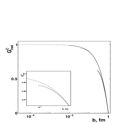
Figure 2: The behavior of $G_{\scriptsize{\mbox{inel}}}^{\,\scriptsize{\mbox{C}}}(s,b)$ using the Coulomb potential, where the full line considers $\sqrt{s_{\scriptsize{\mbox{l.b.}}}}\approx 1.88$ GeV, dotted one $\sqrt{s}=13.8$ GeV, dashed curve $\sqrt{s}=52.8$ GeV and dot-dashed line $\sqrt{s}=14$ TeV. The curves are obtained considering the approximation (18) and $b_{\scriptsize{\mbox{min}}}\leq b\leq b_{\scriptsize{\mbox{max}}}$ with $b_{\scriptsize{\mbox{max}}}=1.0$ fm. Inner panel: the region of the visible difference between two curves at $\sqrt{s}=52.8$ GeV and $\sqrt{s}=14$ TeV.

The Fig. 2 shows the behavior of the inelastic overlap function in accordance with $b_{\scriptsize{\mbox{max}}}$ and for several collision energies from the low-boundary. This boundary is the minimum allowable energy for nucleon-nucleon scattering $\sqrt{s_{\scriptsize{\mbox{l.b.}}}}=2m_{p}$ up to the nominal energy for $pp$ mode at the LHC, where $m_{p}$ is the proton mass PDG-PRD-98-030001-2018 . The choice $b_{\scriptsize{\mbox{max}}}=1$ fm is a result of the typical linear scale of hadron physics.

As been seen above, $G_{\scriptsize{\mbox{inel}}}^{\,\scriptsize{\mbox{C}}}(s,b)$ is characterized by the approximately flat behavior at small $b\lesssim 0.1$ fm, with consequent fast decreasing as $b$ grows for the energy range $\sqrt{s}\gtrsim 14$ GeV. Such behavior may be associated with the absence of an internal structure which is, of course, a result of the naive potential adopted. The weak changing region of $G_{\scriptsize{\mbox{inel}}}^{\,\scriptsize{\mbox{C}}}(s,b)$ narrows with the decreasing of the collision energy.

The inner panel is confirmed and (Fig. 2) shown the region of the visible difference between two curves $G_{\scriptsize{\mbox{inel}}}^{\,\scriptsize{\mbox{C}}}(s,b)$ at $\sqrt{s}=52.8$ GeV (dashed line) and $\sqrt{s}=14$ TeV (dot-dashed line). These features of the behavior of $G_{\scriptsize{\mbox{inel}}}^{\,\scriptsize{\mbox{C}}}(s,b)$ are in full accordance with a detailed analysis of the relation (21).

It is interesting to note that, in the approach of point-like hadrons, as the collision energy increases, $G_{\scriptsize{\mbox{inel}}}^{\,\scriptsize{\mbox{C}}}(s,b)$ shown in Fig. 2, extends to very small values of $b$. Furthermore, the behavior of $G_{\scriptsize{\mbox{inel}}}^{\,\scriptsize{\mbox{C}}}(s,b)$ corresponds to the black disk approach considering $b_{\scriptsize{\mbox{min}}}<b\lesssim 0.10$ fm, and there is no signatures for hollowness effect for any $\sqrt{s}$. At $\sqrt{s}\lesssim 14$ GeV, the inelastic overlap function decreases with the increase of $b$, in almost the entire allowed impact parameter range. The value of $G_{\scriptsize{\mbox{inel}}}^{\,\scriptsize{\mbox{C}}}(s,b)$ is significantly smaller than 1.0 and the black disk approach is not valid in the energy range $\sqrt{s}\lesssim 14$ GeV.

The $b$-dependence of the TE on the Coulomb potential can be immediately derived from the Fig. 2 and relation (20). At qualitative level, the normalized TE, adopting the Coulomb potential $\tilde{S}_{T}^{\,\scriptsize{\mbox{C}}}(s,b)$, is characterized by very small values of $b_{\scriptsize{\mbox{min}}}<b\lesssim 0.10$ fm with fast growth. And $\tilde{S}_{T}^{\,\scriptsize{\mbox{C}}}(s,b)\to 1$ at large enough impact parameter values $b\sim b_{\scriptsize{\mbox{max}}}$, i.e. for peripheral collisions.

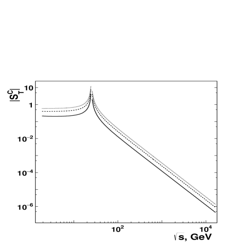
Figure 3: Absolute values of the TE deduced for the Coulomb potential in the impact parameter space, considering $\sqrt{s_{c}}=25.0$ GeV, $b_{\scriptsize{\mbox{min}}}=\sqrt{6/s_{\scriptsize{\mbox{l.b.}}}}$ and $b_{\scriptsize{\mbox{max}}}=10b_{\scriptsize{\mbox{min}}}$. The solid lines correspond to $b=0.5$ fm, dashed one – to the $b=1.0$ fm and dotted lines are for $b=1.5$ fm. Details are described in the text.

In accordance with the general view shown above, the $s$-dependence of the TE for the Coulomb potential is deduced by substituting Eq. (20) into the relation (9). Considering $\sqrt{s_{c}}=25$ GeV and $b<b_{\scriptsize{\mbox{max}}}=\varepsilon_{1}b_{\scriptsize{\mbox{min}}}$, where the $\varepsilon_{1}=10$ and $b_{\scriptsize{\mbox{min}}}$ is defined by $s_{\scriptsize{\mbox{l.b.}}}$, in order to (i) the condition $b_{\scriptsize{\mbox{min}}}\ll b_{\scriptsize{\mbox{max}}}$ be correct and (ii) the whole available energy range for calculation for certain $b$.

The detailed analysis of (9) reveals that $k$ defines the sign of the $\left.S_{T}^{\,\scriptsize{\mbox{C}}}(s,b)\right|_{b=b_{\scriptsize{\mbox{fixed}}}}$, and this quantity shows a sharp behavior for $s\rightarrow s_{c}$. Furthermore, the absolute values of the TE for $s<s_{c}$ ($|S_{T}^{\,\scriptsize{\mbox{C}}}|=-S_{T}^{\,\scriptsize{\mbox{C}}}$) are larger by orders of magnitude than that for $s>s_{c}$ ($|S_{T}^{\,\scriptsize{\mbox{C}}}|=S_{T}^{\,\scriptsize{\mbox{C}}}$). Therefore, the $|S_{T}^{\,\scriptsize{\mbox{C}}}|$ seems the more adequate function for the study of the $s$-dependence of the TE using the approximation (18) for the Coulomb potential in $b$-space.

The energy dependence on the $|S_{T}^{\,\scriptsize{\mbox{C}}}|$ is shown in Fig. 3 for several values of $b$. As expected, the $|S_{T}^{\,\scriptsize{\mbox{C}}}|(s)$ is characterized by a sharp behavior close to the critical energy $s_{c}$, with a subsequent smooth decrease. The $|S_{T}^{\,\scriptsize{\mbox{C}}}|$ assume finite values for $s\to s_{\scriptsize{\mbox{l.b.}}}$ in the energy domain $s<s_{c}$. On the other hand, the absolute value of the TE (9), for the Coulomb potential, decreases significantly with the collision energy growth for $s>s_{c}$ (Fig. 3).

The energy dependence on $|S_{T}^{\,\scriptsize{\mbox{C}}}|$ is mostly defined by the $k$-factor. The influence of the $\tilde{V}_{\scriptsize{\mbox{C}}}(s,b)$ is weak and it only manifests itself at low and intermediate energies: at the low boundary $s_{\scriptsize{\mbox{l.b.}}}$. The relative difference between the exact $\tilde{V}_{\scriptsize{\mbox{C}}}(s,b)$ and the $s$-independent approximation (21) is about 9% for $b=0.5$ fm and $\simeq 0.7$% for $b=1.5$ fm. Moreover, this difference decreases fast as the energy growths and it is negligible ($<0.5$%) for $\sqrt{s}\lesssim 8$ GeV for any considered $b$.

The Coulomb scattering treats the hadrons as billiard balls and does not take into account the influence of the internal arrangement of quarks and gluons for the complete description of the total cross section (or any physical observable). Therefore, any analysis of the elastic scattering should take into account quarks and gluons, which may avoid the occurrence of $b_{\scriptsize{\mbox{min}}}$, presenting a physical explanation of what occurs for $b<b_{\scriptsize{\mbox{min}}}$.

V Confinement Potential

For definition the hadron is considered here as the cold system of quarks and gluons, i.e. as the quark-gluon matter at $T\ll T_{\chi,c}$, where $T_{\chi}$ is the temperature for the chiral symmetry restoration, $T_{c}$ is the temperature for the confinement transition and $T_{\chi,c}\approx 0.15-0.16$ GeV. At such negligibly small temperatures it is customary to obtain the confinement potential ($V_{\scriptsize{\mbox{c}}}$) by adding a linear term to the Coulomb–like potential. Thus, the Coulomb–like part responds by the weak interaction of the antiquark-quark ($\bar{q}q$) pair at short distances while the linear term describes the strong interaction at large distances, i.e. the nature of confinement. As indicated above one supposes the system can be described by the canonical ensemble. In the lowest order, the confinement potential can be written as PRD-17-3090-1978

$$V_{\scriptsize{\mbox{c}}}(\mu,r)=-4\alpha_{s}(\mu)/3r+\kappa r,$$ (22)

where $r$ is now the spatial separation of the pair, strictly speaking, the infinitely heavy (static) quarks and antiquarks inside the hadron. The running coupling constant $\alpha_{s}(\mu)$ is responsible by the strong interaction for a specific energy scale $\mu$ PDG-PRD-98-030001-2018 . The string tension $\kappa$ depends, in general, on the temperature, possessing an average estimation $\sqrt{\kappa}\approx 0.405$ GeV PRD-90-074017-2014 for cold strongly interacting matter. The exact analytic view of the $\alpha_{s}(\mu)$ within the 1-loop approximation is

$$\alpha_{s}(\mu)=(\beta_{0}t)^{-1},$$ (23)

where $t\equiv\ln\bigl{(}\mu^{2}/\Lambda_{\scriptsize{\mbox{QCD}}}^{2}\bigr{)}$, $\beta_{0}=(33-2n_{f})/12\pi$ is the $1$-loop $\beta$-function coefficient, $n_{f}$ is the number of quark flavors active at the energy scale $\mu$, i.e. are considered light $m_{q}\ll\mu$, $m_{q}$ is the quark mass, $\Lambda_{\scriptsize{\mbox{QCD}}}$ is non-universal scale parameter depending on the renormalization scheme adopted, corresponding to the scale where the perturbatively-defined coupling would diverge PDG-PRD-98-030001-2018 .

The numerical value of $\Lambda_{\scriptsize{\mbox{QCD}}}$ depends, in particular, on $n_{f}$ and here one uses $\Lambda_{\scriptsize{\mbox{QCD}}}$ from PDG-PRD-98-030001-2018 , for a given $n_{f}$. At present-day, the convenient estimation of the $\alpha_{s}(\mu)$ is calculated within the complete 5-loop approximation PDG-PRD-98-030001-2018 ; JHEP-1702-090-2017 . Moreover, the running coupling constant can be defined from any physical observable perturbatively calculated grunberg , and for each $\mu$ is obtained a $\alpha_{s}$ resulting in a specific (22).

As seen from (23), one must require $\mu>\mu_{\scriptsize{\mbox{min}}}\equiv\omega\Lambda_{\scriptsize{\mbox{QCD}}}$ to preserve the perturbative definition validity of the coupling $\alpha_{s}(\mu)$. The softest case corresponds to $\omega=1$ while more conservative and exact estimation is given by grunberg

$$\omega=\exp\bigl{[}F_{0}(\alpha_{s}^{\scriptsize{\mbox{max}}})/2\beta_{0}\bigr{]},$$ (24)

where $\alpha_{s}^{\scriptsize{\mbox{max}}}=\beta_{0}/\beta_{1}$, $F_{0}(x)=x^{-1}+\beta_{1}/\beta_{0}\ln(\beta_{0}x)$, $\beta_{1}=(153-9n_{f})/24\pi^{2}$ is the $2$-loop $\beta$-function coefficient PDG-PRD-98-030001-2018 .

There are several estimation of $\mu$ based on $Y_{h}^{\scriptsize{\mbox{exp}}}$, an experimentally measurable quantity. In hadronic collisions, for instance, it is assumed $\mu=Y_{h}^{\scriptsize{\mbox{exp}}}$ at $Y_{h}^{\scriptsize{\mbox{exp}}}\equiv p_{T}^{\scriptsize{\mbox{max}}}$ PRD-86-014022-2012 or $Y_{h}^{\scriptsize{\mbox{exp}}}\equiv m_{3}$ EPJC-75-186-2015 , where $p_{T}^{\scriptsize{\mbox{max}}}$ is the transverse momentum of the leading jet, and $m_{3}$ is the invariant mass of the three jets leading in $p_{T}$.

On the other hand, in the additive quark model J.Nyiri.Int.J.Mod.Phys.A.18.2403.2003 , the $\mu$ scale can be connected with the interaction energy of the leading single $\bar{q}q$-pairs, responsible for the produced particles. The non-leading pairs, called spectators, do not contribute to the particle production EPJC-70-533-2010 . In this picture, the leading particles from the spectators carry away almost all of the collision energy, resulting in that energy has been left for the particle production is about 1/9 of the entire nucleon energy J.Nyiri.Int.J.Mod.Phys.A.18.2403.2003 ; EPJC-70-533-2010 . In a straight analogy, one assumes this corresponds to the scenario for which the $\bar{q}q$-pairs are subject here. Thus, a significant part of the collision energy is absorbed by the spectator $\bar{q}q$-pair, whose contribution to the elastic scattering can be neglected. Then, only part of the collision energy may be used by the (effective) leading $\bar{q}q$-pairs described by the confinement potential. One can note the relation $\mu^{2}\propto s$ is used in general scheme for running coupling in QCD Leader-book-V2-1996 .

Taking into account the above discussion, the energy scale $\mu$ may be connected with $s$ by assuming the simple relation $\mu^{2}=\eta s$ where $0<\eta\leq 1$, which implies that $\mu$ is just a fraction of the energy involved in the elastic scattering process. Taking into account the energy balance in finite-size particles collisions, one can use $\eta=1/9$ J.Nyiri.Int.J.Mod.Phys.A.18.2403.2003 ; EPJC-70-533-2010 , which results in $\mu^{2}=s_{e^{+}e^{-}}$, where $s_{e^{+}e^{-}}$ is the square of the collision energy in $e^{+}e^{-}$ annihilation. The $s_{e^{+}e^{-}}$ is usually used for running coupling in QCD. Moreover, it should point out that assumption connecting the effective energy scale for hadronic collisions ($\mu$ in context of the present work) with $s_{e^{+}e^{-}}$ is not new, being widely and successfully used for decades in many studies, in particular, for the leading effect LNC-38-359-1983, total cross section in nucleon-nucleon collisions PAN-81-508-2018 etc. It should be stressed that $\Lambda_{\scriptsize{\mbox{QCD}}}$ is estimated only for $n_{f}\geq 3$ PDG-PRD-98-030001-2018 . Thus, one can consider $\mu\geq 0.96$ GeV, i.e. $\sqrt{s}\geq 2.88$ GeV based on the perturbatively defined coupling for strong interactions, and taking into account the condition for the lightness of the quark with a certain flavor, as well as the relation between $\mu^{2}$ and $s$ given above. This energy range cover almost all energies allowed for nucleon-nucleon collisions with exception of the narrow region close to the low boundary $\sqrt{s_{\scriptsize{\mbox{l.b.}}}}$.

The assumption performed above is analogous to the momentum fraction $x$ carried by a scattered quark in deep inelastic scattering. The hadron density grows as the energy increases, since there is a change in the fractal dimension of the total cross-section, as proposed in bc . This can be viewed as the parton density increasing, implying the use of very small values for $x$. The cutoff in the parton density growth can be studied by the Balitski–Kovchegov equation, that realizes this saturation through pomeron fan diagrams bartels_braun . On the other hand, as the density grows, the distance narrows between $\bar{q}q$ pairs and within the pairs itself.

The Helmholtz free energy can be understood here in the following way. As the TE increases, the number of degree of freedom of $\bar{q}q$-pairs rise. Thus, the internal energy is given mostly by pairs of particles in the non-confinement regime, i.e. these pairs approach the asymptotic freedom. Then, the entropy term may dominate over the confinement potential and this information should be taken into account in the Helmholtz free energy. However, it is expected this situation may be achieved only near the Hagedorn temperature $T_{c}$. On the other hand, when the entropy diminishes the number of degree of freedom also diminish turning the confinement potential the main energy source. This explanation is the same in the case of the BKT-phase transition in terms of the transition temperature V.L.Berezinskii.Zh.Eksp.Teor.Fiz.59.907.1970 ; J.M.Kosterlitz.D.J.Thouless.J.Phys.C6.1181.1973 . Below the transition temperature, the potential energy dominates, preventing the emergence of a single vortex. Otherwise, the entropy is favored, turning possible the presence of a single vortex state.

V.1 Confinement potential in $b$-space and normalization procedure

The confinement potential is of short-range in contrast with the Coulomb one and, by reason of the uncertainty principle, the quantity $\mu_{\scriptsize{\mbox{min}}}$ allows the unambiguous estimation of the linear scale $r_{\scriptsize{\mbox{max}}}\sim\mu_{\scriptsize{\mbox{min}}}^{-1}$, up to which the confinement potential can be calculated with help of (22). One can expect $r_{\scriptsize{\mbox{max}}}\sim R_{h}$, depending on the approach for $\mu_{\scriptsize{\mbox{min}}}$ and on the values of the $\Lambda_{\scriptsize{\mbox{QCD}}}$ at given $n_{f}$ PDG-PRD-98-030001-2018 , where $R_{h}$ is the hadron radius. This upper cutoff for $r$ tames the divergence of the confinement potential (22). In general, one should considers $b\leq b_{\scriptsize{\mbox{max}}}\sim r_{\scriptsize{\mbox{max}}}$ for the incoming particles interacting by strong force with each other. Table 1 shows the values for $b_{\scriptsize{\mbox{max}}}=\mu_{\scriptsize{\mbox{min}}}^{-1}$ calculated for various numbers of light quark flavor and schemes, aiming the definition of the low boundary for the domain on $\mu$ in which the perturbative definition of the coupling $\alpha_{s}(\mu)$ is valid. As seen, $b_{\scriptsize{\mbox{max}}}$ is significantly smaller within a conservative scheme for $\mu_{\scriptsize{\mbox{min}}}$ than that for softest one at any fixed $n_{f}$ and values of $b_{\scriptsize{\mbox{max}}}$ are in the range from about 0.59 (0.37) fm at $\sqrt{s}=2.88$ GeV to the $\simeq 2.22$ (1.44) fm at the nominal LHC energy $\sqrt{s}=14$ TeV for the softest (conservative) restriction on the $\mu_{\scriptsize{\mbox{min}}}$. As expected $b_{\scriptsize{\mbox{max}}}(s)$ is constant at fixed $n_{f}$ with sharply increasing at growth of $n_{f}$. The step magnitude increases with the onset of the influence of heavier flavors, being largest for the transition from $n_{f}=5$ to $n_{f}=6$. On the other hand, a smaller space scale $r\to 0$ inside the hadron can be probed through more central collisions, with $b\to 0$. Within the general framework of the paper, the relation $b_{\scriptsize{\mbox{min}}}\sim\mu^{-1}=(\eta s)^{-1/2}$ is used for a rough estimation of the lower boundary for the impact parameter at a given $s$. Therefore, one can assume $r=\varepsilon_{3}b$, where $\varepsilon_{3}\leq 1$, and the confinement potential in the impact parameter space can be rewritten as

$$V_{\scriptsize{\mbox{c}}}(\mu,r)=V_{\scriptsize{\mbox{c}}}(s,b)=-4\alpha_{s}(\eta s)/3\varepsilon_{3}b+\kappa\varepsilon_{3}b.$$ (25)

The potential $V_{\scriptsize{\mbox{c}}}(\mu,r)$ and $V_{\scriptsize{\mbox{c}}}(s,b)$ coincide exactly in whole domain $(\mu\geq\mu_{\scriptsize{\mbox{min}}};r\leq r_{\scriptsize{\mbox{max}}}$), due to exact (linear) interrelations between the corresponding terms in the parameter pairs $(\mu,r)$ and $(s,b)$. Note the Coulomb-like term in $V_{\scriptsize{\mbox{c}}}(s,b)$ behaves as $V_{\scriptsize{\mbox{C}}}(s,b)\approx-ab^{-1}$ for a sufficient high fixed-$s$. However, in $V_{\scriptsize{\mbox{c}}}(s,b)$ the information about $s$ is embodied in the running coupling.

Taking into account the general properties of hadronic collisions discussed above, for the sake of simplicity, one uses $\varepsilon_{3}=1.0$ unless otherwise specifically indicated. As seen the confinement potential (25) is null at

$$b_{0}=\sqrt{4\alpha_{s}(\eta s)/3\kappa}\propto\sqrt{\alpha_{s}(\eta s)},$$ (26)

where the allowable ranges are taken into account for the linear scales $r$ and $b$, i.e. $r,b>0$. Table 2 shows the values of $b_{0}$ calculated for various $n_{f}$ within 1- and 5-loop approximation for $\alpha_{s}(\mu)$ at two collision energies considered in the present work. Transition from the intermediate energy $\sqrt{s}=52.8$ GeV to the high one $\sqrt{s}=14$ TeV significantly reduces $b_{0}$ from $\sim 0.21-0.24$ fm down to $\sim 0.14-0.16$ fm at fixed $n_{f}$. The increase in the number of light quark flavors results in the growth of $b_{0}$ for some collision energies, whereas the use of higher-order approximation for $\alpha_{s}(\mu)$ provides smaller values of $b_{0}$ at fixed $n_{f}$ and $s$. It is interesting to note that it can be shown that $b_{0}\gtrsim b_{\scriptsize{\mbox{max}}}$ at $\sqrt{s}\approx 2.88$ GeV for $\omega$ defined by (24) and 5-loop approximation, i.e. in this case $\forall\,b:V_{\scriptsize{\mbox{c}}}(s,b)<0$, in the very narrow energy range close to the lowest allowed value of $s$.

Thus the detailed analysis shows that the characteristic linear scales in the impact parameter space – $b_{\scriptsize{\mbox{min}}}$, $b_{0}$ and $b_{\scriptsize{\mbox{max}}}$ – are $s$-dependent. There is also a dependence on the scheme for the estimation of $\mu_{\scriptsize{\mbox{min}}}$ for the $b_{\scriptsize{\mbox{max}}}$ (Table 1) as well as there is a relies on the number of loops for $\alpha_{s}(\eta s)$ approximation for $b_{0}$ (Table 2).

Table 1: Maximum values of the impact parameter for perturbative approach ($b_{\scriptsize{\mbox{max}}}$, fm)

Scheme for $\mu_{\scriptsize{\mbox{min}}}$	$n_{f}$
	3	4	5	6
softest ($\omega=1$)	$0.59\pm 0.03$	$0.68\pm 0.04$	$0.94\pm 0.06$	$2.22\pm 0.15$
conservative ($\omega>1$)	$0.365\pm 0.019$	$0.418\pm 0.023$	$0.59\pm 0.04$	$1.44\pm 0.10$

Table 2: Values of $b_{0}$ (fm) at two collision energies

Approximation	$n_{f}$
order for $\alpha_{s}(\mu)$	3	4	5	6
$\sqrt{s}=52.8$ GeV
1-loop	$0.2359\pm 0.0015$	$0.2413\pm 0.0016$
5-loop	$0.2134\pm 0.0012$	$0.2199\pm 0.0013$
$\sqrt{s}=14$ TeV
1-loop	$0.1521\pm 0.0004$	$0.1570\pm 0.0004$	$0.1610\pm 0.0005$	$0.1617\pm 0.0005$
5-loop	$0.1433\pm 0.0004$	$0.1486\pm 0.0004$	$0.1534\pm 0.0005$	$0.1558\pm 0.0005$

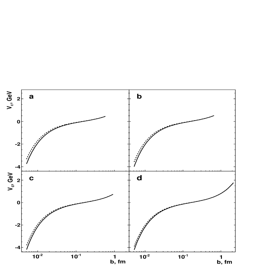
Figure 4: Dependence of the confinement potential at $\sqrt{s}=14$ TeV and $n_{f}=3$ (a), $n_{f}=4$ (b), $n_{f}=5$ (c) and $n_{f}=6$ (d) with various approximations for $\alpha_{s}(\mu)$: solid line is for the 1-loop solution (23) and dashed curve corresponds to the 5-loop approximation PDG-PRD-98-030001-2018 . The softest scheme for $\mu_{\scriptsize{\mbox{min}}}$ is used without loss of generality.

Contrary to the Coulomb potential, the confinement allows a glance at the hadron internal arrangement, revealing its importance for the correct description of the elastic scattering, even in this naive potential approach. The Fig. 4 shows the $b$-dependence of the confinement potential (25) for fixed $\sqrt{s}=14$ TeV and various numbers of the light flavors $n_{f}$ for 1- and 5-loop approximation for $\alpha_{s}(\mu)$. The value $\omega=1$ is used for definition of the $\mu_{\scriptsize{\mbox{min}}}$ and, consequently, the largest value of the upper cutoff for $b$.

The 5-loop approximation for $\alpha_{s}(\mu)$ provides slightly larger values of $V_{\scriptsize{\mbox{c}}}(s,b)$ than that for 1-loop exact solution (23) only in the range of small values $b\lesssim 0.03$ fm (not shown here). The consistent transition from Fig. 4a to Fig. 4d shows the weakening of the difference between the two curves with the growth of $n_{f}$. Thus, in general the approximation order for $\alpha_{s}(\mu)$ influences weakly on the $V_{\scriptsize{\mbox{c}}}(s,b)$ in the whole range of $b$ for any $n_{f}$ considered, and the results are stable with respect to the scheme of calculation for $\alpha_{s}(\mu)$. By definition, the modern 5-loop approximation can be used for $\alpha_{s}(\mu)$ below, unless otherwise indicated. At the intermediate energy $\sqrt{s}=52.8$ GeV, $V_{\scriptsize{\mbox{c}}}(s,b)$ does not depend on the number of light flavors (Figs. 5a, b). The confinement potential dependence on $n_{f}$ manifests itself only in the high energy domain, for instance at $\sqrt{s}=14$ TeV, in which the wide set of the values of $n_{f}$ is available (Figs. 5c, d). In the last case, the growth of $n_{f}$ has provided some decrease in $V_{\scriptsize{\mbox{c}}}(s,b)$ for small $b\lesssim 0.03$ fm as expected, expanding the confinement potential for larger impact parameter values $b\gtrsim R_{h}$ due to the decrease of $\Lambda_{\scriptsize{\mbox{QCD}}}$.

The modification in the scheme to estimate of $\mu_{\scriptsize{\mbox{min}}}$ does not influence on the functional behavior of the $V_{\scriptsize{\mbox{c}}}(s,b)$, for both the intermediate (Figs. 5a, b) and the high energy (Figs. 5c, d) considered here. The transition from $\omega=1$ (Figs. 5a c) to the conservative estimation of this parameter (Figs. 5b, d), leads to the decrease of the high boundaries for linear scales $r$ and $b$. The Fig. 6 shows the evolution of the $V_{\scriptsize{\mbox{c}}}(s,b)$ considering the collision energy growth for fixed $n_{f}=3$ (a, b) and $n_{f}=4$ (c, d) for two different approaches for $\mu_{\scriptsize{\mbox{min}}}$. As seen before, $V_{\scriptsize{\mbox{c}}}(s,b)$ is larger for $\sqrt{s}=14$ TeV than that for $\sqrt{s}=52.8$ GeV at corresponding values of $b$, for any number of light flavors $n_{f}$ and scheme for the $\omega$-parameter calculation. Furthermore, the difference between the two curves increases as $b$ decreases. The behavior of $V_{\scriptsize{\mbox{c}}}(s,b)$ in Fig. 6 is explained by the smooth decreasing of $\alpha_{s}(\mu)$ with the growth of $\mu$ PDG-PRD-98-030001-2018 , i.e. with the collision energy growth due to the relation used here.

In general, the main features of the confinement potential shown in Figs. 4 – 6 are driven by contributions coming from different terms in (22) or, consequently, (25) for several ranges of the impact parameter values. The $V_{\scriptsize{\mbox{c}}}(s,b)$ is sensitive for changes in $n_{f}$, $s$ and mostly for small $b$, since the main contribution in this range comes from the first (short-range) term in (25) containing $\alpha_{s}(\mu)$ that depends, in turn, on $n_{f}$ and $s$. The influence of the first term decreases as $b$ grows as well as the contribution of the second (long-range) term becomes dominant in (25). This term depends on string tension only and, consequently, $V_{\scriptsize{\mbox{c}}}(s,b)$ it is not sensitive for $n_{f}$ and changes weakly with $s$, for relatively large $b>0.1$ fm. Here, changes of $n_{f}$ and / or $s$ provides different values for the up boundary $b_{\scriptsize{\mbox{max}}}$ for $b$–range considered perturbatively.

Figure 5: Dependence of the confinement potential on impact parameter at $\sqrt{s}=52.8$ GeV (a, b) and $\sqrt{s}=14$ TeV (c, d) for various $n_{f}$: solid line is for $n_{f}=3$, dashed one – for $n_{f}=4$, dotted curve corresponds to the $n_{f}=5$ and dot-dashed one – to the $n_{f}=6$. The left column (a, c) shows results for $\omega=1$ and curves for conservative estimation (24) are in the right column (b, d).

Figure 6: Dependence of the confinement potential on impact parameter at $n_{f}=3$ (a, b) and $n_{f}=4$ (c, d) for two collision energies: solid line is for $\sqrt{s}=52.8$ GeV and dashed one – for $\sqrt{s}=14$ TeV. The left column (a, c) shows results for $\omega=1$ and curves for conservative estimation (24) are in the right column (b, d).

It is necessary to normalize the potential (25) to obey the unitarity condition. As well-known, the second term in (22) as well as (25) provides the main difference between the confinement potential and the Coulomb one, namely, the positive values and the quasi-linear growth of the $V_{\scriptsize{\mbox{c}}}(s,b)$ at large $b$, i.e. $r$ (Figs. 4 – 6). If one considers the equation (19) and taking into account the appropriate values of $\gamma$, then the confinement potential has a constant sign within the $b$-range under consideration. However, in general, the potential $V(s,b)$ may change its sign within the kinematic domain studied and this feature can lead to the discontinuity for $\tilde{V}(s,b)$, if extremum (maximum) value of the $V(s,b)$ is used as the scale factor. The analysis performed shows that using the maximum for the absolute value of the potential, then $|V(s,b)|_{\scriptsize{\mbox{max}}}$ avoids the possible discontinuity in the behavior of the $\tilde{V}(s,b)$, in the case of sign changing of $V(s,b)$. Therefore, here the following relation is used

$$\tilde{V}_{\scriptsize{\mbox{c}}}(s,b)=|V_{\scriptsize{\mbox{c}}}(s,b)|/|V_{\scriptsize{\mbox{c}}}(s,b)|_{\scriptsize{\mbox{max}}}.$$ (27)

where $|V_{\scriptsize{\mbox{c}}}(s,b)|$ is the absolute value of the confinement potential $V_{\scriptsize{\mbox{c}}}(s,b)$, if the confinement potential changes its sign within the $b$-range under discussion. In this case, the $|V_{\scriptsize{\mbox{c}}}(s,b)|_{\scriptsize{\mbox{max}}}$ can be reached at low or high boundary of $b$ (Figs. 4 – 6). Without loss of generality, the range $b_{\scriptsize{\mbox{min}}}\leq b\leq b_{\scriptsize{\mbox{max}}}$ is studied below, where $V_{\scriptsize{\mbox{c}}}(s,b_{\scriptsize{\mbox{min}}})<0$ and $b_{\scriptsize{\mbox{max}}}$ is controlled by $r_{\scriptsize{\mbox{max}}}$. Thus, the normalized confinement potential, on the impact parameter space, can be written as

$$\tilde{V}_{\scriptsize{\mbox{c}}}(s,b)=\frac{b}{b_{\scriptsize{\mbox{n}}}}\biggl{|}\frac{1-[4\alpha_{s}(\eta s)/3\kappa]b^{-2}}{1-[4\alpha_{s}(\eta s)/3\kappa]b_{\scriptsize{\mbox{n}}}^{-2}}\biggr{|}=\frac{b}{b_{\scriptsize{\mbox{n}}}}\biggl{|}\frac{1-(b_{0}/b)^{2}}{1-(b_{0}/b_{\scriptsize{\mbox{n}}})^{2}}\biggr{|},$$ (28)

where

$$b_{\scriptsize{\mbox{n}}}=\left\{\begin{array}[]{lcl}b_{\scriptsize{\mbox{min}}},&\mbox{if}&|V_{\scriptsize{\mbox{c}}}(s,b_{\scriptsize{\mbox{min}}})|>V_{\scriptsize{\mbox{c}}}(s,b_{\scriptsize{\mbox{max}}});\vspace{0.2cm}\\ b_{\scriptsize{\mbox{max}}},&\mbox{if}&|V_{\scriptsize{\mbox{c}}}(s,b_{\scriptsize{\mbox{min}}})|\leq V_{\scriptsize{\mbox{c}}}(s,b_{\scriptsize{\mbox{max}}}).\\ \end{array}\right.$$ (31)

The confinement potential is still assumed as featured by finite negative value for $b_{\scriptsize{\mbox{min}}}$.

As seen above, $V_{\scriptsize{\mbox{c}}}(s,b_{\scriptsize{\mbox{max}}})<2$ GeV for any loop approximation (Fig. 4), scheme for $\mu_{\scriptsize{\mbox{min}}}$ estimation, and $n_{f}$ values (Fig. 5). Consequently, the condition $|V_{\scriptsize{\mbox{c}}}(s,b)|_{\scriptsize{\mbox{max}}}=V_{\scriptsize{\mbox{c}}}(s,b_{\scriptsize{\mbox{max}}})$ is valid up to $b_{\scriptsize{\mbox{min}}}\gtrsim 10^{-2}$ fm. Therefore, the lower relation in (31) is, in general, applicable, while the upper equation in (31) is valid only for processes that probe the inner structure of a hadron down to the very small linear scales.

V.2 Inelasticity and TE for the strong interaction

Results are shown in Fig. 7 for detailed analysis of the dependence of $\tilde{V}_{\scriptsize{\mbox{c}}}(s,b)$ on the impact parameter for several $s$, $n_{f}$ and ranges $b\in[b_{\scriptsize{\mbox{min}}},b_{\scriptsize{\mbox{max}}}]$. The softest scheme for $\mu_{\scriptsize{\mbox{min}}}$ is used, without loss of generality. In Fig. 7a the relations $b_{\scriptsize{\mbox{n}}}=b_{\scriptsize{\mbox{max}}}\gg b_{0}$ are valid. In this case

$$\tilde{V}_{\scriptsize{\mbox{c}}}(s,b)\approx b\bigl{[}1-(b_{0}/b)^{2}\bigr{]}/b_{\scriptsize{\mbox{max}}}.$$

Here the $n_{f}$– and $s$–dependencies survive in $\tilde{V}_{\scriptsize{\mbox{c}}}(s,b)$ due to $b_{0}$ and $b_{\scriptsize{\mbox{max}}}$. These dependencies are seen most clearly in Fig. 7b. The minimum of $\tilde{V}_{\scriptsize{\mbox{c}}}(s,b)$ goes to the smaller $b$ with the increase of the dip for larger $s$ and fixed $n_{f}$, in accordance with the dependence $\alpha_{s}(\eta s)$. The relations $b_{\scriptsize{\mbox{n}}}=b_{\scriptsize{\mbox{min}}}\ll b_{0}$ are valid in Figs. 7c, d. Then

$$\tilde{V}_{\scriptsize{\mbox{c}}}(s,b)\approx bb_{\scriptsize{\mbox{min}}}\bigl{[}1-(b_{0}/b)^{2}\bigr{]}/b_{0}^{2}.$$

This equation allows two asymptotic cases: (i) $\bigl{.}\tilde{V}_{\scriptsize{\mbox{c}}}(s,b)\bigr{|}_{b\to b_{\scriptsize{\mbox{min}}}\ll b_{0}}\to b_{\scriptsize{\mbox{min}}}/b$ and (ii) $\bigl{.}\tilde{V}_{\scriptsize{\mbox{c}}}(s,b)\bigr{|}_{b\to b_{\scriptsize{\mbox{max}}}\gg b_{0}}\to bb_{\scriptsize{\mbox{min}}}/b_{0}^{2}$. As can be seen above, there are no $n_{f}$– and $s$–dependencies of the normalized confinement potential for values of $b$ close to the down boundary $b_{\scriptsize{\mbox{min}}}$ of the considered range. At large $b\to b_{\scriptsize{\mbox{max}}}$, the energy and $n_{f}$–dependencies display itself due to $b_{0}$ but these dependencies are (very) weak because of (very) small $b_{\scriptsize{\mbox{min}}}$. The parameter $b_{\scriptsize{\mbox{max}}}$ is most sensitive for changes of $n_{f}$ and / or $s$. Figs. 7c, d confirm the results for the asymptotic behavior of $\tilde{V}_{\scriptsize{\mbox{c}}}(s,b)$ in the cases (i) and (ii).

Therefore, the general conclusions follow from relations (28) in the domain of validity of the condition $b_{\scriptsize{\mbox{min}}}\ll b_{0}$. The normalized confinement potential and corresponding inelastic overlap function $G_{\scriptsize{\mbox{inel}}}^{\,\scriptsize{\mbox{c}}}(s,b)$ are weakly sensitive on changes of the $n_{f}$ and $s$, and the energy dependence of the TE $S_{T}^{\,\scriptsize{\mbox{c}}}$ is driven by $k$.

Based on the Fig. 7, $b_{\scriptsize{\mbox{min}}}=0.05$ fm is used in order to show clearly the $n_{f}$– and $s$–dependencies of the inelastic overlap function for confinement potential.

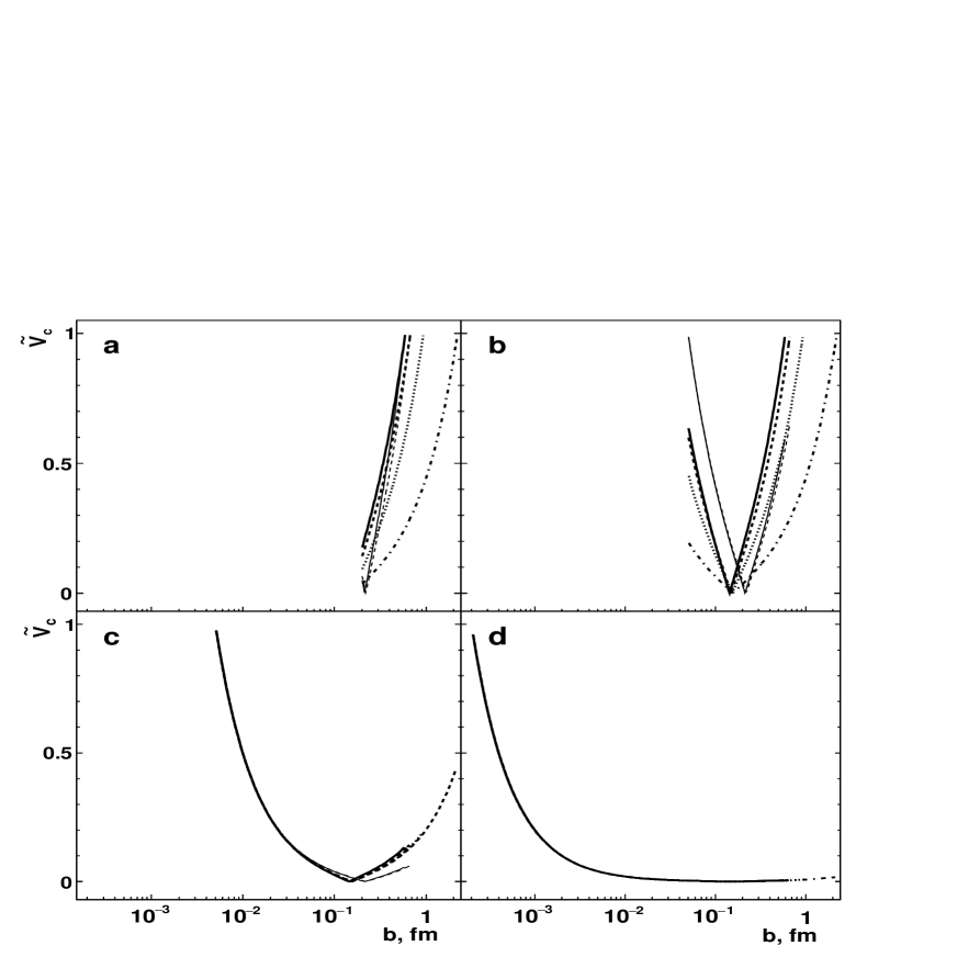
Figure 7: Dependence of the normalized confinement potential on impact parameter with the following values of the low boundary for $b$–range under studied: $0.2$ fm (a), $0.05$ fm (b), $5\times 10^{-3}$ fm (c) and $2\times 10^{-4}$ fm (d). Are considered two collision energies $\sqrt{s}=52.8$ GeV (thin lines) and $\sqrt{s}=14$ TeV (thick curves). The $\tilde{V}_{\scriptsize{\mbox{c}}}(s,b)$ are shown for $\omega=1$ and solid lines are for $n_{f}=3$, dashed ones – for $n_{f}=4$, dotted curves correspond to the $n_{f}=5$ and dot-dashed ones – to the $n_{f}=6$.

The Fig. 8 shows the dependence of the inelastic overlap function for the confinement potential $G_{\scriptsize{\mbox{inel}}}^{\,\scriptsize{\mbox{c}}}(s,b)$ on $b$ for several $n_{f}$ and approaches for $\omega$ for two collision energies $\sqrt{s}=52.8$ GeV (a, b) and 14 TeV (c, d). The scheme for estimation of $\omega$ does not influence on the $G_{\scriptsize{\mbox{inel}}}^{\,\scriptsize{\mbox{c}}}(s,b)$ for intermediate energies (Fig. 8a, b). However, the situation changes at $\sqrt{s}=14$ TeV (Fig. 8c, d): the conservative estimation for $\omega$ leads to smaller $G_{\scriptsize{\mbox{inel}}}^{\,\scriptsize{\mbox{c}}}(s,b)$ at $b<b_{0}$, in comparison with the case for $\omega=1$, and the influence is weaker for larger $n_{f}$. The influence of $n_{f}$ on the view of $G_{\scriptsize{\mbox{inel}}}^{\,\scriptsize{\mbox{c}}}(s,b)$ is negligible at $\sqrt{s}=52.8$ GeV (Fig. 8a, b), and the growth of the number of light flavors leads to the increase of $G_{\scriptsize{\mbox{inel}}}^{\,\scriptsize{\mbox{c}}}(s,b)$ at fixed $b$ for $\sqrt{s}=14$ TeV (Fig. 8c, d), especially for large $n_{f}=5$ and 6. For the confinement potential, the black disk regime $G_{\scriptsize{\mbox{inel}}}^{\,\scriptsize{\mbox{c}}}(s,b)\approx 1$ is reached at $b_{0}$ and in the region close to this inflection point of the $V_{\scriptsize{\mbox{c}}}(s,b)$. As discussed above, this region expands as $n_{f}$ grows, especially for the largest $n_{f}=6$. Such behavior agrees with the expectation for qualitative expansion of the region with high absorption in the nucleon-nucleon collisions at higher energies. On the other hand, the general feature of the $G_{\scriptsize{\mbox{inel}}}^{\,\scriptsize{\mbox{c}}}(s,b)$ in Fig. 8 is the more transparent (gray) regions for both the small ($b\ll b_{0}$) and the large ($b\gg b_{0}$) impact parameters.

The Fig. 9 shows $G_{\scriptsize{\mbox{inel}}}^{\,\scriptsize{\mbox{c}}}(s,b)$, depending on $b$ for several $\sqrt{s}$ and approaches for $\omega$, considering two different numbers of light flavors $n_{f}=3$ (a, b) and 4 (c, d). The behavior of $G_{\scriptsize{\mbox{inel}}}^{\,\scriptsize{\mbox{c}}}(s,b)$ at $\sqrt{s}=14$ TeV, depending on the scheme for the estimation of $\omega$, leads to different relations between the two inelastic overlap functions at $n_{f}=3$ in Figs. 9a and 9b, at $n_{f}=4$ in Figs. 9c and 9d. The maximum of $G_{\scriptsize{\mbox{inel}}}^{\,\scriptsize{\mbox{c}}}(s,b)$ tends to the smaller $b\simeq 0.15$ fm as $\sqrt{s}$ increase. At $\omega=1$, the $G_{\scriptsize{\mbox{inel}}}^{\,\scriptsize{\mbox{c}}}(s,b)$ is significantly larger at $\sqrt{s}=14$ TeV than for $\sqrt{s}=52.8$ GeV at $b\lesssim 0.15$ fm, and vice versa at larger $b\gtrsim 0.3$ fm, for both the $n_{f}=3$ (Fig. 9a) and the $n_{f}=4$ (Fig. 9c). Thus, the stronger absorption region shifts to the smaller $b$, i.e. appear in more central collisions at $\sqrt{s}=14$ TeV with regard of the corresponding region at intermediate energy $\sqrt{s}=52.8$ GeV. Adopting the conservative estimation (24), the behavior of the maximum of $G_{\scriptsize{\mbox{inel}}}^{\,\scriptsize{\mbox{c}}}(s,b)$ is the same in dependence of the $\sqrt{s}$. Nonetheless, the excess of the inelastic overlap function at $\sqrt{s}=14$ TeV over the quantity at $\sqrt{s}=52.8$ GeV is seen in a significantly narrower region $0.07\lesssim b\lesssim 0.15$ fm. The relation is the opposite between these overlap functions for larger $b$ and near the behavior of $G_{\scriptsize{\mbox{inel}}}^{\,\scriptsize{\mbox{c}}}(s,b)|_{\sqrt{s}=52.8\,\scriptsize{\mbox{GeV}}}$ and $G_{\scriptsize{\mbox{inel}}}^{\,\scriptsize{\mbox{c}}}(s,b)|_{\sqrt{s}=14\,\scriptsize{\mbox{TeV}}}$ for smaller $b$. These statements are valid at $n_{f}=3$ (Fig. 9b) and at $n_{f}=4$ (Fig. 9). Thus, the conservative scheme for the $\omega$ lead to the hollowness effect for both very different energies considered here.

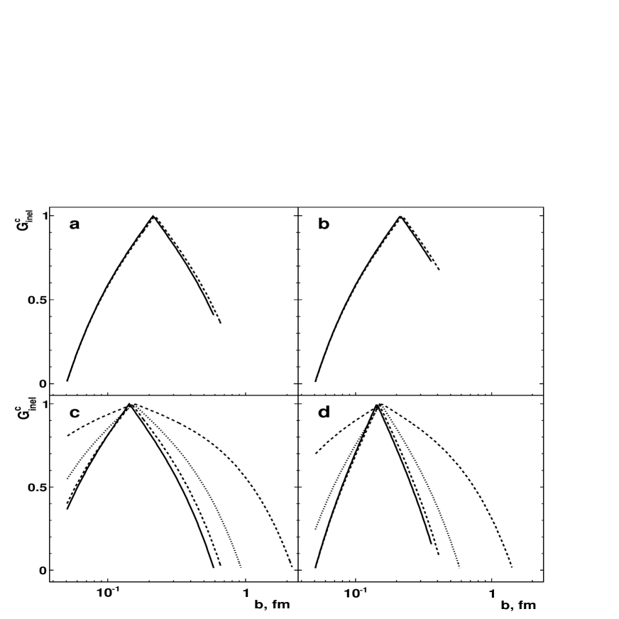
Figure 8: Behavior of $G_{\scriptsize{\mbox{inel}}}^{\,\scriptsize{\mbox{c}}}(s,b)$ using the confinement potential at $b_{\scriptsize{\mbox{min}}}=0.05$ fm, $\sqrt{s}=52.8$ GeV (a, b) and $\sqrt{s}=14$ TeV (c, d) for various $n_{f}$: solid line is for $n_{f}=3$, dashed one – for $n_{f}=4$, dotted curve corresponds to the $n_{f}=5$ and dot-dashed one – to the $n_{f}=6$. The left column (a, c) shows results for $\omega=1$ and curves for conservative estimation (24) are in the right column (b, d).

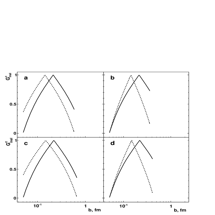
Figure 9: Behavior of $G_{\scriptsize{\mbox{inel}}}^{\,\scriptsize{\mbox{c}}}(s,b)$ using the confinement potential at $b_{\scriptsize{\mbox{min}}}=0.05$ fm, $n_{f}=3$ (a, b) and $n_{f}=4$ (c, d) for two collision energies: solid line is for $\sqrt{s}=52.8$ GeV and dashed one – for $\sqrt{s}=14$ TeV. The left column (a, c) shows results for $\omega=1$ and curves for conservative estimation (24) are in the right column (b, d).

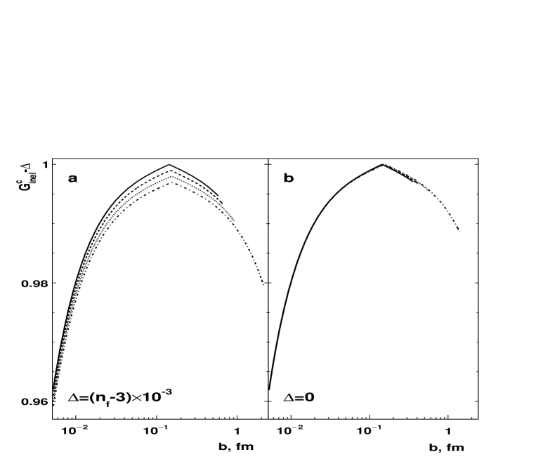
Figure 10: Dependence of $G_{\scriptsize{\mbox{inel}}}^{\,\scriptsize{\mbox{c}}}$ on $b$ for the confinement potential at $b_{\scriptsize{\mbox{min}}}=2.0\times 10^{-4}$ fm and $\sqrt{s}=14$ TeV for various $n_{f}$ with $\omega=1$ (a) and conservative estimation (24) used for $\mu_{\scriptsize{\mbox{min}}}$ (b). The solid lines are for $n_{f}=3$, dashed ones – for $n_{f}=4$, dotted curves correspond to the $n_{f}=5$ and dot-dashed ones – to the $n_{f}=6$. The curves are shifted on the finite $\Delta$ in (a) for clearness.

All curves shown in the Figs. 8 and 9 reveal the presence of a critical value $b_{0}$, in agreement with the analyses performed, revealing the existence of a gray area for $b<b_{0}$. As above mentioned, the $b_{\scriptsize{\mbox{min}}}=0.05$ fm is mostly chosen for the display of $n_{f}$– and $s$–dependencies for $G_{\scriptsize{\mbox{inel}}}^{\,\scriptsize{\mbox{c}}}$. As expected from Fig. 7, the view of $b$–dependence of the inelastic overlap function for the confinement potential changes with $b_{\scriptsize{\mbox{min}}}$ dramatically. Fig. 10 shows the $G_{\scriptsize{\mbox{inel}}}^{\,\scriptsize{\mbox{c}}}(b)$ at very small $b_{\scriptsize{\mbox{min}}}=2\times 10^{-4}$ fm, $\sqrt{s}=14$ TeV and several $n_{f}$ for $\omega=1$ (a) and conservative estimation (24) used for $\mu_{\scriptsize{\mbox{min}}}$ (b). Accounting for the absence of visible $n_{f}$–dependence in Fig. 7d, the curves for various $n_{f}$ are shifted on finite $\Delta$ in Fig. 10a. At present the $b_{\scriptsize{\mbox{min}}}=2\times 10^{-4}$ fm can be considered as quite reasonable approximation for $b=0$. In this case $G_{\scriptsize{\mbox{inel}}}^{\,\scriptsize{\mbox{c}}}(b)$ shows the approaching for the black disk limit at accuracy level $\approx 2\%$ for $b$ varying in wide range $10^{-2}$ fm $\lesssim b\leq b_{\scriptsize{\mbox{max}}}$. The range of $b$ in which $G_{\scriptsize{\mbox{inel}}}^{\,\scriptsize{\mbox{c}}}(b)\approx 1$ is expanded significantly for $b_{\scriptsize{\mbox{min}}}=2\times 10^{-4}$ fm in comparison with Figs. 8 and 9. However, $G_{\scriptsize{\mbox{inel}}}^{\,\scriptsize{\mbox{c}}}(b)$ also decreases sharply in the narrow region close to the $b_{\scriptsize{\mbox{min}}}$ in this case (Fig. 10).

Thus, the results shown in Figs. 8–10 allows the following general conclusions. First of all, notice that inelastic overlap function description, based on the confinement potential, exhibits the black disk limit for $b\neq 0$ and a clear gray area emerging near $b=0$ (the hollowness effect). The gray area narrows with the decreasing of $b_{\scriptsize{\mbox{min}}}$ but it survives for any finite values of the parameter $b_{\scriptsize{\mbox{min}}}$. Then, the hollowness effect can be considered an essential and intrinsic feature of the confinement potential approach. It should be stressed that the potentials $V_{\scriptsize{\mbox{c}}}(s,b)$ and sequential $\tilde{V}_{\scriptsize{\mbox{c}}}(s,b)$ can be applied to describe the interaction of color-charged constituents, strictly speaking. At present, the self-consistent description from the first principles of QCD is absent for the transition from the quark-gluon plasma to the hadronic matter. Actually, there is an important hypothesis of local parton–hadron duality (LPHD) suggesting that the hadronization preserves the main features of the partonic interactions at hadronic level, i.e. the so-called soft hadronization ZPC-27-65-1985 . Nevertheless, the hadronization can influence and (slightly) distort a distribution for some quantities at experimentally measurable (hadronic) level, concerning the corresponding distributions for partonic interactions. Furthermore, one may suggest this influence can be amplified in some kinematic domain. Obviously, this is only a qualitative hypothesis which should be justified and verified by quantitative estimations. But, in any case, the comparison is possible at a qualitative level for $G_{\scriptsize{\mbox{inel}}}^{\,\scriptsize{\mbox{c}}}(s,b)$ obtained taking into account the confinement potential and the experimental results for hadronic (in particular, $pp$ and $\bar{p}p$) collisions. Considering the above and within the understanding that the use of confinement potential is a naive approach for $G_{\scriptsize{\mbox{inel}}}^{\,\scriptsize{\mbox{c}}}(s,b)$, one can make a qualitative comparison between the results of present work with some other phenomenological approaches.

In general, the behavior of $G_{\scriptsize{\mbox{inel}}}^{\,\scriptsize{\mbox{c}}}(s,b)$ in Fig. 8, obtained taking into account the potential approach, confirms the results from dremin_1 ; dremin_2 and analyses done by broniowski_arriola ; alkin_martynov ; anisovich_nikonov ; troshin_tyurin_1 ; anisovich ; troshin_tyurin_2 ; albacete_sotoontoso ; arriola_broniowski . Furthermore, one expects that the inelastic overlap function description holds better for small values of $b$. In particular, the behavior of $G_{\scriptsize{\mbox{inel}}}^{\,\scriptsize{\mbox{c}}}(b)$ in Fig. 10 shows the minimum at $b\to 0$ which is quite similar to the shallow minimum $G_{\scriptsize{\mbox{inel}}}^{\,\scriptsize{\mbox{c}}}(b)\simeq 0.97-0.98$ for most central bin $b\in[0.0;0.1]$ fm, obtained within mass squared approach with central optical potential at the same $\sqrt{s}=14$ TeV arriola_broniowski . Also there is the second characteristic displayed by the hollowness effect in Fig. 10, namely the shift of the maximum to larger $b=b_{0}$ but $G_{\scriptsize{\mbox{inel}}}^{\,\scriptsize{\mbox{c}}}(b)$, obtained for hadronic level, shows a flatter growth and a wide maximum at $b\simeq 0.4-0.5$ fm arriola_broniowski . Therefore, the confinement potential provides the hollowness effect on central collisions at the nominal LHC energy $\sqrt{s}=14$ TeV (Fig. 8c, d), as obtained by another method for $pp$ collisions arriola_broniowski . Furthermore, the analysis of high-statistic data close to $\sqrt{s}=13$ TeV and taking into account the Lévy imaging T.Csorgo.R.Pasechnik.A.Ster.Euro.Phys.J.C80.126.2020 , results in a noticeably shallower minimum for $G_{\scriptsize{\mbox{inel}}}^{\,\scriptsize{\mbox{c}}}(0)=0.9915\pm 0.0008$ at $b\leq 0.05$ fm and the maximum shifts to $b\simeq 0.4$ fm. But the last result does not contradict the prediction in Fig. 10, at qualitative level.

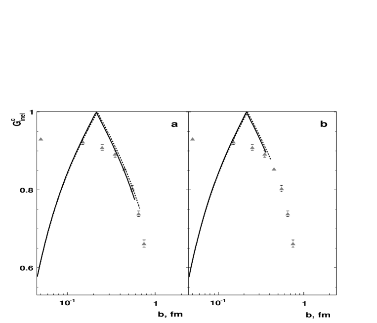
Figure 11: Dependence of $G_{\scriptsize{\mbox{inel}}}^{\,\scriptsize{\mbox{c}}}$ on $b$ for the confinement potential at $b_{\scriptsize{\mbox{min}}}=2.0\times 10^{-2}$ fm and $\sqrt{s}=52.8$ GeV for various $n_{f}$ with $\omega=1$ (a) and conservative estimation (24) used for $\mu_{\scriptsize{\mbox{min}}}$ (b) in comparison with the results for $pp$ collisions at same $\sqrt{s}$ from NPB-166-301-1980 shown by triangles. The solid lines are for $n_{f}=3$, dashed ones – for $n_{f}=4$.

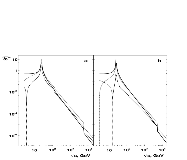
Figure 12: Absolute values of the TE deduced for confinement potential in the impact parameter space on collisions energy considering $b_{\scriptsize{\mbox{min}}}=0.05$ fm, $\sqrt{s_{c}}=25.0$ GeV, softest (a) and conservative (b) restriction on the $\mu_{\scriptsize{\mbox{min}}}$. The solid lines are for $b=0.10$ fm while dashed curve corresponds to the $b=0.35$ fm in (a) and $b=0.25$ fm in (b), dotted lines are for $b=0.60$ fm (a) and 0.40 fm (b).

It is known the shape of the $G_{\scriptsize{\mbox{inel}}}(b)$ is model-dependent. Fig. 11 shows of $G_{\scriptsize{\mbox{inel}}}^{\,\scriptsize{\mbox{c}}}$ on $b$ calculated within the present work for the confinement potential at $b_{\scriptsize{\mbox{min}}}=2.0\times 10^{-2}$ fm and $\sqrt{s}=52.8$ GeV for various $n_{f}$ for soft (a) and conservative (b) estimation used for $\mu_{\scriptsize{\mbox{min}}}$ and results derived with help of the another approach elsewhere NPB-166-301-1980 . As discussed above the behavior of $G_{\scriptsize{\mbox{inel}}}^{\,\scriptsize{\mbox{c}}}(b)$ depends on the free parameter $b_{\scriptsize{\mbox{min}}}$. Therefore there is some arbitrariness at choosing a value of this parameter for certain $\sqrt{s}$. This uncertainty can be excluded, for instance, with help of the fit by (16) some reliable data. The value $b_{\scriptsize{\mbox{min}}}=2.0\times 10^{-2}$ fm is chosen empirically because the definition of the best value of $b_{\scriptsize{\mbox{min}}}$ for certain $\sqrt{s}$ is outside the subject of the present work. The approach for $G_{\scriptsize{\mbox{inel}}}^{\,\scriptsize{\mbox{c}}}(b)$ based on the perturbative confinement potential provides the quantitative agreement with the results from NPB-166-301-1980 at $b\gtrsim 0.3$ fm for $\omega=1$ (Fig. 11a). The indication on the similar conclusion can be only suggested for Fig. 11b because of one point from NPB-166-301-1980 is in the region of overlap of two models at $b\gtrsim 0.3$ fm. Predictions of two models differ dramatically at smaller $b$: the present approach shows the maximum for $G_{\scriptsize{\mbox{inel}}}^{\,\scriptsize{\mbox{c}}}(b)$ at $b\sim 0.2$ fm with subsequent decrease while the results from NPB-166-301-1980 are smoothly increase. It means the hollowness effect within the present approach based on the $\tilde{V}_{\scriptsize{\mbox{c}}}(s,b)$ defined by (28) and absence of the effect for data points from NPB-166-301-1980 . As qualitatively discussed above, the hadronization can influence on the view of $G_{\scriptsize{\mbox{inel}}}^{\,\scriptsize{\mbox{c}}}(b)$. Thus, the hadronization may explain, at least some part, the difference of the inelastic overlap function for quark and hadronic levels, in addition to the ambiguous choice of the $b_{\scriptsize{\mbox{min}}}$. It is interesting to note that the smooth approximations within the method from sdcvaocvm demonstrate a noticeable deviation from the level $G_{\scriptsize{\mbox{inel}}}^{\scriptsize{\mbox{max}}}(s,0)=1$ in the energy domain from $\sqrt{s}\simeq 20$ GeV up to $\sqrt{s}\sim 100$ GeV for $pp$, $\bar{p}p$ and the combined sample for nucleon-nucleon scattering.

The $b$-dependence of the TE for confinement potential ($S_{T}^{\,\scriptsize{\mbox{c}}}$) is driven by the Figs. 8, 9 and relation (20).

Likewise the Coulomb potential, the sign of the $S_{T}^{\,\scriptsize{\mbox{c}}}$ is defined by $k$ due to the normalization procedure. Furthermore, the TE for the confinement potential is featured by sharply changes near $s_{c}$. The absolute values of the TE for $s<s_{c}$ ($|S_{T}^{\,\scriptsize{\mbox{c}}}|=-S_{T}^{\,\scriptsize{\mbox{c}}}$) are larger by orders of magnitude than that for $s>s_{c}$ ($|S_{T}^{\,\scriptsize{\mbox{c}}}|=S_{T}^{\,\scriptsize{\mbox{c}}}$). Then, as well as in Sec. IV, the $|S_{T}^{\,\scriptsize{\mbox{c}}}|$ is the adequate quantity for study of $s$-dependence of the TE for the approximation (25) of the confinement potential in $b$-space.

The Fig. 12 shows the energy behavior of the TE absolute value for the confinement potential within the 5-loop approximation for $\alpha_{s}$ at $b_{\scriptsize{\mbox{min}}}=0.05$ fm, $\sqrt{s_{c}}=25.0$ GeV, softest (a) and conservative (b) restriction on the $\mu_{\scriptsize{\mbox{min}}}$ for several $b$. The additional analysis shows that $|S_{T}^{\,\scriptsize{\mbox{c}}}|(s,b)$ does not depend on the scheme for the estimation of $\omega$ at a given value of the impact parameter. Thus, the values of $b$ differ in Fig. 12a and 12b for most cases. As expected, the factor $k$ provides similar general trends for the energy dependence of the TE in Fig. 12 in comparison with Fig. 3. However, the behavior of $|S_{T}^{\,\scriptsize{\mbox{c}}}(s,b)|$ is more intricate than that for the Coulomb potential. The very sharp minimums are the $|S_{T}^{\,\scriptsize{\mbox{c}}}(s,b)|=0$ at $\sqrt{s}$ for which $b=b_{0}$. As discussed above, the sharp changing of the $|S_{T}^{\,\scriptsize{\mbox{c}}}(s,b)|$ due to onset of influence of heavier flavors is most visible for $n_{f}=6$ in TeV-energy range.

VI Discussions and Conclusions

The presence of the hollowness effect (gray area) cannot be associated with limiting the resolution of the facilities. On the other hand, the de Broglie wavelength achieves its minimum at present-day energies at the LHC, and despite its small value $\Delta r=1/p_{cm}\sim 2/\sqrt{s}$ it still produces an unavoidable natural coarse-grain effect.

The use of potentials mimicking the internal energy is not new in physics, probably remounting to Bohm quantum potential bohm_1 ; G.Dennis.M.A.de.Gosson.B.J.Hiley.Phys.Lett.A378.2363.2014 in Quantum Mechanics and, more specifically, in nuclear scattering Shuryak-book-2004-p374 . However, the use of both the Coulomb and the confinement potentials are illustrative of the physical behavior of $pp$ and $\bar{p}p$ in the impact parameter space. It should be stressed that the confinement potential was applied here at the level of the charged-color particles. Moreover, the hadronization can influence and distort distributions at the hadronic level despite the LPHD hypothesis. Therefore the results obtained in the resent work are not able to fit the experimental data for the inelastic overlap function since this is not the aim of a potential approach.

The Coulomb potential treats the hadrons as point-like objects, and its description using the impact parameter picture does not allow any acceptable result near the forward direction. Far from the forward direction (high $q^{2}$), derivative terms can also be added to achieve a better description of the inelastic overlap function introducing a slowdown decaying for the tail (low $q^{2}$).

On the other hand, the confinement potential considered here as the internal energy of the hadron shows the hollowness effect in a qualitative level. Thus, the confinement potential may allow the rise of this effect even if we add derivative terms (corresponding to the tail). It is important to stress that, using a different approaches, the hollowness effect was recently predicted at the LHC energies $\sqrt{s}=7$ arriola_broniowski 13 PRD-98-074012-2018 ; T.Csorgo.R.Pasechnik.A.Ster.Euro.Phys.J.C80.126.2020 and 14 TeV arriola_broniowski .

The physical behavior expressed by the confinement potential represents an intrinsic feature of the strong interaction. Then, the confinement potential approach furnishes the qualitative general behavior of the inelastic overlap function. The results shown in Figs. 8 – 10 represent the impossibility to ascribe to the inelastic overlap function only one exponential sdcvaocvm ; D.A.Fagundes.M.J.Menon.P.V.R.G.Silva.Nucl.Phys.A946.194.2016 . The presence of a persistent maximum even in the energy region where it is not expected can be attributed to the inevitable normalization procedure (see Fig. 11). Then, one expects the cuspid behavior can be smoothed for low energies. Otherwise, the cuspid becomes pronounced as the energy rise. Note this behavior is absent in the Coulomb approach.

In order to avoid the hollowness effect, from the confinement point of view, we should modify the confinement potential adding correction terms acting only near the forward direction. These terms may correspond, for example, to kinematic terms emerging at a very high $q^{2}$ (very short distance). However, it seems unlikely since corrections to the linear term of (25) imply or in the decreasing of the strength of the confinement potential to $b\rightarrow 0$ or simply not modifying its general behavior as $b\rightarrow 0$ (or introducing some noise or small perturbations). None of these assumptions seems to be physically reasonable. Therefore, we claim here that the presence of a gray area in the impact parameter space is a consequence of the thermodynamic processes as well as of the multifractal character of the hadron in the energy and momentum spaces.

The entropy probably is one of the most important physical quantities in nature and should be taken into account in all physics explanations. In the TE, the entropic index $w$ is replaced by a convenient choice of parameters representing a phase transition occurring at $s=s_{c}$, in total cross-section experimental data-set. The probability density function is replaced by the inelastic overlap function in the impact parameter space. This convenient form of entropy provides an understanding of how the matter density induces the geometric pattern observed in the $pp$ and $\bar{p}p$ elastic scattering.

The increasing or decreasing entropy implies in an increasing or decreasing probability of the inelastic overlap function, which result is the emergence of a critical value $b_{0}$ associated with the matter distribution inside $pp$ and $\bar{p}p$ elastic scattering. Therefore, the entropy determines the existence of the critical value in the impact parameter space. The consequence of this result may be viewed as the presence of a fractal character in the momentum space antoniou_1 ; antoniou_2 ; antoniou_4 ; antoniou_5 ; bialas_1 ; bialas_2 .

Of course, the TE is one of several one ways to compute the entropy of a non-additive system. However, without loss of generality, the cases of interest can be reduced to the Tsallis form, even the additive entropies by taking $w=1$ beck_0902.1235v2 ; tsallis_book .

The $\bar{q}q$-interaction entails the energy density distribution inside the proton and may determine the emergence of the hollowness effect. Recently, the $k$-factor was introduced to take into account the phase transition occurring in the total cross section furnishing an explanation for the radial pressure distribution in the proton S.D.Campos.Int.J.Mod.Phys.A34.1950057.2019 . A possible consequence that result is the emergence of the hollowness effect manifested in the von Laue stability condition M.von.Laue.Annalen.der.Physik.340.(8).524.1911 .

Finally, the analyses carried out here are based on few physical assumptions and allows one to obtain the occurrence of the gray area in the inelastic overlap function without the use of models for the $pp$ and $\bar{p}p$ elastic scattering. It should be emphasized that the approach presented is not able to furnish any best fitting result of any experimental data, since this is not its aim, which is the qualitative study of both the possible phase transition in the total cross section and the existence of a gray area in the inelastic overlap function. Bearing this in mind, the results obtained can help in the construction of models taking into account the existence of both physical phenomena in the $pp$ and $\bar{p}p$ elastic scattering.

References

- (1) Report on the physics at the HL–LHC, and perspectives for the HE–LHC. Eds. A. Dainese, M. Mangano, A. B. Meyer et al. CERN Yellow report: monographs. CERN–2019–007. CERN, Geneva (2019).
- (2) V. V. Anisovich, V. A. Nikonov and J. Nyiri, Phys. Rev. D90, 074005 (2014).
- (3) V. V. Anisovich, M. A. Matveev and V.A. Nikonov, Int. J. Mod. Phys. A31, 1645019 (2016); G. Pancheri and Y. N. Srivastava, Eur. Phys. J. C77, 3 (2017).
- (4) S. D. Campos, V. A. Okorokov and C. V. Moraes, Phys. Scr. 95, 025301 (2020).
- (5) H. Cheng and T. T. Wu, Expanding protons: scattering at high energies. The MIT Press (1987); A. Donnachie, H. G. Dosch, P. V. Landshoff and O. Nachmann, Pomeron physics and QCD. Cambridge Univ. Press (2002).
- (6) V. Barone and E. Predazzi, High-energy particle diffraction. Springer–Verlag (2002).
- (7) I. M. Dremin, Phys. Uspekhi 58, 61 (2015).
- (8) I. M. Dremin Phys. Uspekhi 60, 333 (2017).
- (9) W. Broniowski and E. Ruiz Arriola, Acta Phys. Polon. B10 Proc. Supp., 1203 (2017).
- (10) A. Alkin, E. Martinov, O. Kovalenko and S. M. Troshin, Phys. Rev. D89, 091501 (2014).
- (11) S. M. Troshin and N. E. Tyurin, Int. J. Mod. Phys. A29, 1450151 (2014).
- (12) V. V. Anisovich, Phys. Uspekhi 58, 963 (2015).
- (13) S. M. Troshin and N. E. Tyurin, Mod. Phys. Lett. A31, 1650079 (2016).
- (14) J. L. Albacete and A. Soto-Ontoso, Phys. Lett. B770, 149 (2017).
- (15) E. Ruiz Arriola and W. Broniowski, Phys. Rev. D95, 074030 (2017).
- (16) F. S. Borcsik and S. D. Campos, Mod. Phys. Lett. A31, 1650066 (2016).
- (17) C. Tsallis, Braz. J. Phys. 39, 337 (2009).
- (18) N. G. Antoniou, F. Diakonos and C. G. Papadopoulos, Phys. Lett. B265, 399 (1991).
- (19) N. G. Antoniou, V. E. Zambetakis, F. K. Diakonos, and N. K. Diakonou, Z. Phys. C55, 631 (1992).
- (20) N. G. Antoniou, F. Diakonos, I. S. Mistakidis and C. G. Papadopoulos, Phys. Rev. D49, 5789 (1994).
- (21) N. G. Antoniou, N. Davis, and F. K. Diakonos, Phys. Rev. C93, 014908 (2015).
- (22) A. Bialas, Nucl. Phys. A545, 285c (1992).
- (23) A. Bialas, Acta Phys. Pol. B23, 561 (1992).
- (24) A. Deppman, Phys. Rev. D93, 054001 (2016).
- (25) S. D. Campos, Phys. Scr. 95, 065302 (2020).
- (26) S. D. Campos, arXiv: 2003.11493 [hep-ph] (2020).
- (27) M. Froissart, Phys. Rev. 123, 1053 (1961).
- (28) L. Lukaszuk and A. Martin, Nuovo Cim. A52, 122 (1967).
- (29) A. Martin, Phys. Rev. D80, 065013 (2009).
- (30) T. T. Wu, A. Martin, S. M. Roy, and V. Singh, Phys. Rev. D84, 025012 (2011).
- (31) A. Martin and S. M. Roy, Phys. Rev. D91, 076006 (2015).
- (32) V. A. Okorokov, Phys. At. Nucl. 82, 134 (2019).
- (33) U. Amaldi and K. R. Schubert, Nucl. Phys. B166, 301 (1980).
- (34) R. Henzi and P. Valin, Phys. Lett. B132, 443 (1983).
- (35) R. Henzi and P. Valin, Phys. Lett. B160, 167 (1985).
- (36) A. Alkin, E. Martynov, O. Kovalenko and S. M. Troshin, Phys. Rev. D89, 051901 (2014).
- (37) W. Broniowski, L. Jenkovszky, E. Ruiz Arriola and I. Szanyi, Phys. Rev. D98, 074012 (2018).
- (38) T. Csörgő, R. Pasechnik and A. Ster, Eur. Phys. J. C80, 126 (2020).
- (39) G. Antchev et al. (TOTEM Collaboration), Eur. Phys. J. C79, 861 (2019).
- (40) I. M. Dremin and V. A. Nechitailo, Eur. Phys. J. C78, 913 (2018).
- (41) A. Rényi, in Proceedings of the IV Berkeley Symposium on mathematical statistics and probability, 1, 547 (1960).
- (42) C. E. Shannon, Bell Sys. Tech. J. 27, 379 (1948).
- (43) S. Abe, Phys. Lett. A224, 326 (1997).
- (44) C. Beck, Contemporary Phys. 50, 495 (2009).
- (45) C. Tsallis, Introduction to nonextensive statistical mechanics: approaching a complex world. Springer Science (2009).
- (46) C. Tsallis, R. S. Mendes and A.R. Plastino, Phys. A261, 534 (1998).
- (47) B. G. Levich, Theoretical physics: an advanced text. 2, John Wiley & Sons, Inc. (1971).
- (48) J. I. Kapusta and G. Charles, Finite-temperature field theory principles and applications. Cambridge Univ. Press (2006).
- (49) M. Kaufman, Principles of Thermodynamics. Marcel Dekker, Inc. (2001).
- (50) E. V. Shuryak, The QCD vacuum, hadrons and superdense matter. Lec. Notes Phys. 71, World Scientific (2004) and references therein.
- (51) E. V. Shuryak and I. Zahed, Phys. Rev. D70, 054507 (2004).
- (52) F. Karsch, AIP Conf. Proc. 602, 323 (2001).
- (53) O. Kaczmarek et al., Prog. Theor. Phys. Supp. 153, 287 (2004); O. Kaczmarek and F. Zantow, PoS (LAT2005), 192 (2005); Y. Burnier, O. Kaczmarek and A. Rothkopf, Phys. Rev. Lett. 114, 082001 (2015); P. Petreczky, A. Rothkopf and J. Weber, Nucl. Phys. A982, 735 (2019).
- (54) Shuai Y. F. Liu and R. Rapp, Nucl. Phys. A941, 179 (2015); Phys. Rev. C97, 034918 (2018); Shuai Y. F. Liu, Min He and R. Rapp, ibid 99, 055201 (2019).
- (55) G. Dennis, M. A. de Gosson and B. J. Hiley, Phys. Lett. A378, 2363 (2014); ibid 379, 1224 (2015).
- (56) N. F. Ramsey, Phys. Rev. 103, 10 (1956).
- (57) E. Eichten et al., Phys. Rev. D17, 3090 (1978).
- (58) M. Tanabashi et al., Phys. Rev. D98, 030001 (2018).
- (59) A. P. Trawinski et al., Phys. Rev. D90, 074017 (2014).
- (60) F. Herzog, J. High Energy Phys. 02, 090 (2017); P. A. Baikov, K. G. Chetyrkin and J. H. Khn, Phys. Rev. Lett. 118, 082002 (2017).
- (61) G. Grunberg, Phys. Lett. 95B, 70 (1980).
- (62) G. Aad et al. (ATLAS Collaboration), Phys. Rev. D86, 014022 (2012); V. Khachatryan et al. (CMS Collaboration), Eur. Phys. J. C75, 288 (2015).
- (63) V. Khachatryan et al. (CMS Collaboration), Eur. Phys. J. C75, 186 (2015).
- (64) E. Leader and E. Predazzi E, An introduction to gauge theories and modern particle physics. 2, Cambridge Univ. Press (1996).
- (65) J. Nyiri, Int. J. Mod. Phys. A18, 2403 (2003).
- (66) E. K. G. Sarkisyan and A. S. Sakharov, Eur. Phys. J. C70, 533 (2010); E. K. G. Sarkisyan, A. N. Mishra, R. Sahoo, and A. S. Sakharov, Phys. Rev. D93, 054046 (2016).
- (67) M. Basile et al., Lett. Nuovo Cimen. 38, 359 (1983).
- (68) V. A. Okorokov, Phys. At. Nucl. 81, 508 (2018).
- (69) J. Bartels and M. A. Braun, J. High Energy Phys. 06, 095 (2018).
- (70) V. L. Berezinskii, Sov. Phys. JETP 32, 493 (1971).
- (71) J. M. Kosterlitz and D. J. Thouless, J. Phys. C6, 1181 (1973).
- (72) D. A. Fagundes, M. J. Menon and P. V. R. G. Silva, Nucl. Phys. A946, 194 (2016).
- (73) Ya. I. Azimov, Yu. L. Dokshitzer, V. A. Khoze and S. I. Troyan, Z. Phys. C27, 65 (1985).
- (74) D. Bohm, Phys. Rev. 85, 166 (1952); ibid, 180 (1952).
- (75) S. D. Campos, Int. J. Mod. Phys. A34, 1950057 (2019).
- (76) M. von Laue, Ann. der Phys. 340, 524 (1911).