Which is better, a SCoTSS gamma imager, or an ARDUO UAV-borne directional detector?

Abstract

The SiPM-based Compton Telescope for Safety and Security (SCoTSS) has been developed with inorganic crystalline scintillator material for gamma detection. The instrument is sensitive enough to be used in a mobile survey mode, accumulating energy deposited in any crystal second-by-second and tagging these spectra with GPS position. The SCoTSS imager of course has the additional advantage of being able to produce an image of the radioactive objects in its field of view using events that satisfy a coincidence trigger between the scatter and absorber layers. The Advanced Radiation Detector for UAV Operations (ARDUO) on the other hand, is a non-imaging directional detector intended for use aboard a small unmanned aerial vehicle (UAV). The ARDUO detector features exactly the same volume of CsI(Tl) as is used in the absorber layer of a single SCoTSS module, giving it similar detection and alarming sensitivity, and map-making capability. However, in the ARDUO detector, the crystals are arranged closely together to optimize direction determination from self-shielding effects. Flown in a grid pattern with a UAV over an area of extended contamination, the ARDUO detector is also capable of making a map or image of that area. With its close-packed crystal arrangement, the ARDUO detector makes a poor Compton imager but does have some ability to produce a peripheral image in a fly-by. In this presentation we investigate the relative merits of Compton imaging versus mobile directional detection.

I Introduction

The detection of ionizing radiation emitted by radioactive material using instruments employing scintillating crystals and light sensors has a long history [1]. Radionuclide identification is typically performed by examining peaks found in the measured energy spectrum and comparing them to known radionuclide emission lines. For a stationary detector, the measurement of the radiation directionality, and thus the localization of the radioactive material, can be achieved through the use of passive absorbing material (e.g. collimation, coded aperture, etc), active absorbing material (e.g. self-shielding) or through kinematic interactions (e.g. Compton scattering). Surveying with a non-stationary instrument allows for localization by simply measuring the activity at a variety of points over some spatial region. These localization methods, by their very nature, have intrinsic strengths and weaknesses which make them particularly well suited, or ill suited, to specific applications.

We have developed two instruments based on thallium-doped cesium iodide CsI(Tl) crystal scintillators coupled to silicon photomultiplier (SiPM) light sensors. While both instruments employ almost identical sensing and read-out components and have similar mass, one is configured as a Compton imaging telescope and the other as a non-imaging self-shielding directional detector. Access to both these instruments affords us a unique opportunity to examine and compare their performance in a variety of deployment settings. In these proceedings we describe our findings based on our study of these instruments.

(a) SCoTSS Compton imager

(b) ARDUO directional detector

Figure 1: Schematic renderings of the active components of the two detectors. The SCoTSS Compton imager module is composed of two layers, each segmented into 4$\times$4 crystal arrays. The ARDUO directional detector is arranged as a close-packed segmented tower with two 2$\times$2 crystal arrays. To account for the different instrument sizes, image scales are unequal. The scintillator mass used in ARDUO is identical to the scintillator mass used in SCoTSS absorber (rear) layer.

II Instruments

II-A Compton Imager - SCoTSS

The SiPM-based Compton Telescope for Safety and Security, SCoTSS, is a Compton imaging radiation detector comprised of CsI(Tl) crystal scintillators coupled to silicon photomultiplier light sensors [2]. Simulation studies and prototyping development over many years [3, 4] have led us to a design with two segmented layers. A “scatter layer”, positioned at the front of the detector, is designed to ensure Compton scatter interactions yield excellent positional and energy resolution, while minimizing the probability of multiple scatters within the front layer. This layer is composed of cubic crystals, 1.35 cm on a side, mated to SiPMs manufactured by SensL Technologies Ltd using optical gel. The second layer, the “absorber layer”, employs cubic crystals 2.8 cm on a side, also mated to SiPMs. This layer is designed to absorb all of the remaining energy of gamma rays which scattered in the front layer, while achieving the required level of positional resolution. These two segmented sensor layers, connected with custom designed coincidence-timing and read-out electronics, provide all the information needed to use the Compton equation [5] to determine the incident angle of gamma rays which scatter in the first layer and are fully absorbed in the second.

The SCoTSS instrument is designed to be modular, with a single module employing a 4$\times$4 array of crystals in the scatter layer and a 4$\times$4 array in the absorber layer (see Figure 1a). This design allows for different configurations of SCoTSS modules to be combined and arranged depending on what is suitable and practical in a given deployment setting. In this work, however, only a single SCoTSS module is considered.

II-B Self-shielding directional detector - ARDUO

The Advanced Radiation Detector for Unmanned Aerial Vehicle Operations, ARDUO, is a directional gamma-ray detector arranged as a close-packed segmented tower with two 2$\times$2 CsI(Tl) scintillator crystal arrays (see Figure 1b). The crystals are 2.8 cm $\times$ 2.8 cm $\times$ 5.6 cm in size and mated with the same SiPM optical sensors used in the SCoTSS instrument. The direction to a source is determined through a self-shielding method. Light is collected in the scintillator crystals in the same way as is employed in the SCoTSS module, however, energy deposits are accumulated into one-second duration histograms and coincidence information is not utilized. Using the relative rate of energy depositions in each crystal a range of algorithms can be utilized to find the most likely direction to a source of emission.

Both the SCoTSS and ARDUO detectors use power supplies and read-out electronics custom built by our partners at Radiation Solutions Inc. ARDUO has an active volume the same as that of the SCoTSS absorber layer and their sensor components are read out with very similar acquisition electronics. Their particular configuration is therefore the principle difference between these two instruments. This allows us to directly compare their performance using a range of methods across a variety of deployment scenarios.

Source Type	ARDUO	SCoTSS
	Localization Methods	Localization Methods
Point	Response-function search	Response-function search
		Compton-cone fit†
Extended	Rate survey	Rate survey
	Simple direction finding	Back projection†
	Response-function fit	Response-function fit

TABLE I: Summary of the localization and directional methods used in this study. The ${\dagger}$ symbol indicates methods which require coincidence timing.

Point-source results

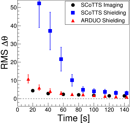
(a) RMS deviation against time [10^∘ offset]

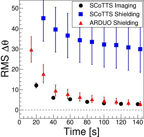
(b) RMS deviation against time [60^∘ offset]

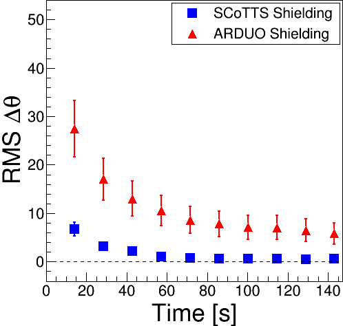
(c) RMS deviation against time [90^∘ offset]

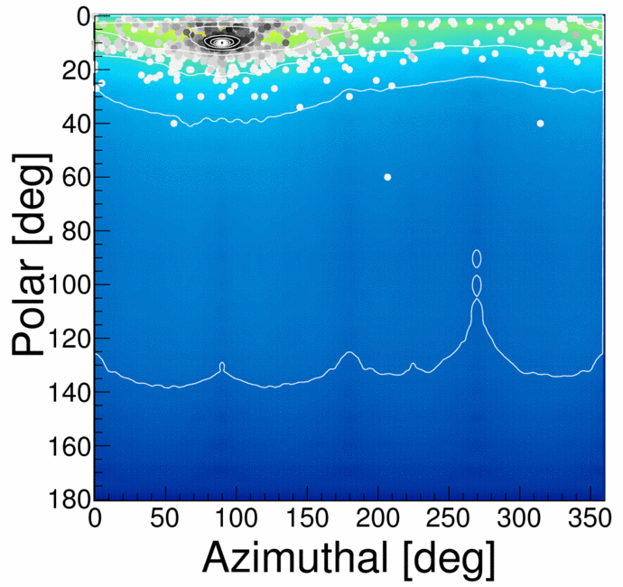
(d) ARDUO likelihood [10^∘ offset]

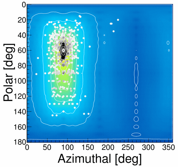
(e) ARDUO likelihood [60^∘ offset]

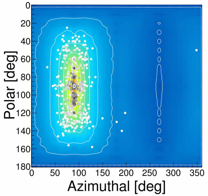
(f) ARDUO likelihood [90^∘ offset]

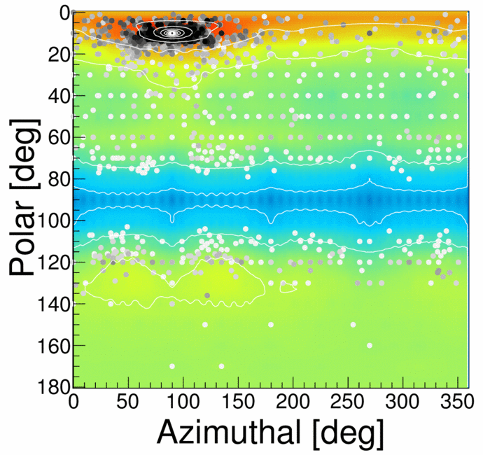
(g) SCoTSS likelihood [10^∘ offset]

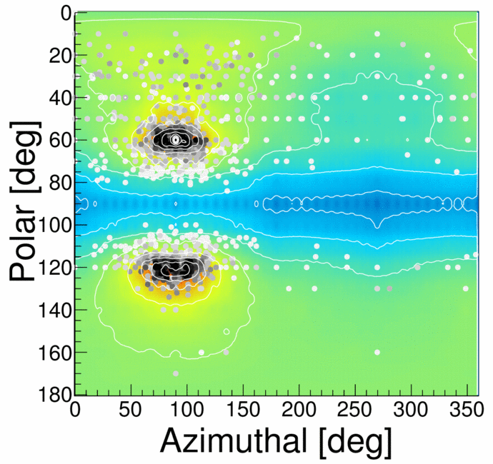
(h) SCoTSS likelihood [60^∘ offset]

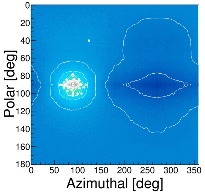
(i) SCoTSS likelihood [90^∘ offset]

Figure 2: Reconstruction of a simulated 1 mCi ¹³⁷Cs point source located at an offset distance of 10 m using self-shielding and Compton imaging methods. Panels (a-c) show the root-mean-squared (RMS) deviation of the reconstructed direction to a point source versus accumulation time. The response-function search self-shielding method (triangles and squares) can be compared to the Compton-cone fit method (circles). The circular symbols in panels (d-f) show individual ARDUO self-shielding reconstructions, with their colour (from light-grey to black) indicating the acquisition time. The colour map indicates the likelihood that the self-shielding algorithm will reconstruct a given position in 4$\pi$ phase space when the true position is located at an azimuth of 90^∘ and a polar angle given in the individual sub-caption (see text Section IV-B1). Panels (g-i) show the equivalent information for the SCoTSS self-shielding reconstructions. Notable is the likelihood information in panel (h), indicating that the crystal configuration in the SCoTSS instrument yields areas of the response function look-up-table which are self-similar, leading to erroneous reconstructions which do not significantly improve with accumulation time. This is directly responsible for the large RMS of the SCoTSS self-shielding reconstruction plotted in panel (b).

III Experimental Setup

To examine and compare the performance of the SCoTSS and ARDUO detectors we perform a range of simulation studies using the Geant4 [6] and EGSnrc simulation packages [7, 8]. Both detectors are simulated in the presence of point-like and distributed sources of photons emitted at 662 keV - simulating the response to gamma-ray emission from ¹³⁷Cs. Data acquired with SCoTSS and ARDUO exposed to calibrated ¹³⁷Cs sources are used to verify our simulations, but not shown in this work.

III-A Point source

The point-like source studies examine the detector response to a 1 mCi ¹³⁷Cs source located at an offset distance of 10 m and positioned at a range of angles from the principle detector axes.

III-B Distributed source

We simulated 150 m $\times$ 150 m aerial grid surveys of distributed sources located 10 m below the detectors. Grid points are separated by 10 m in both easting and northing corresponding to a flight speed of 10 m/s and line spacing of 10 m. Two distributed-source sizes were studied, one at the 100 m size scale consisting of an L-shaped source with a 10 m $\times$ 60 m northing section and a 70 m $\times$ 5 m easting section (see Figures 3a, c and e). The second distributed source, 10 times smaller than the first, consists of an L-shaped source with a 1 m $\times$ 6 m northing section and a 7 m $\times$ 0.5 m easting section (see Figures 3b, d and f).

Table I summarizes the range of directional and imaging methods investigated in this work.

IV Method

IV-A Non-directional method - Rate survey

This method does not use the individual rate information of each detector crystal, but simply the total rate of energy deposits, and plots this total rate against the location in the grid survey. Results based on this method are used in the distributed-source studies plotted in Figure 3a and Figure 3b.

IV-B Self-shielding directional methods

Self-shielding directional methods use the rate of energy deposits in each scintillator crystal to determine the most likely direction to the source of emission. One can imagine a simple case of two crystals side by side - crystal A on the left of crystal B. If, in the presence of a source, the rate in crystal A is much higher than that in B then one can infer that a source is located somewhere to the left of B, since A is shielding B from the flux of incident events. A range of methods based on the (relative) rate of energy deposits are used in this study.

IV-B1 Response-function search

Simulation datasets are computed with point sources located at a range of angular positions covering the 4$\pi$ angular phase space around the detector at some offset distance. Interpolating this dataset one can construct look-up tables (LUT) of the detector response, $S_{i}(\theta,\phi)$, indicating the expected relative rate in crystal $i$ in the presence of a point source positioned at polar coordinate angles $(\theta,\phi)$. To localize a source at some unknown position, the LUTs are searched to find the $(\theta,\phi)$-point where the detector response is most similar to the measured rates.

The similarities between the detector response at one $(\theta,\phi)$-point compared to another, $(\theta^{\prime},\phi^{\prime})$, is indicative of the likelihood that this algorithm will reconstruct the source location to be at $(\theta^{\prime},\phi^{\prime})$, when the true position is at the location $(\theta,\phi)$. As a proxy for this likelihood, we compute the $N$-dimensional distance in LUT rate-space between $(\theta,\phi)$ and $(\theta^{\prime},\phi^{\prime})$,

$$D(\theta^{\prime},\phi^{\prime})=\sqrt{\sum_{i=1}^{N}(S_{i}(\theta,\phi)-S_{i}(\theta^{\prime},\phi^{\prime}))^{2}}$$

where $N$ is the number of crystals. This quantity allows us to assess the self-shielding directional characteristics of a given detector configuration from the LUT. For examples of the use of this distance metric see the colour map in Figures 2d-i.

IV-B2 Simple direction finding

One starts by choosing three perpendicular axes in the detector geometry, e.g. “top-bottom”, “left-right” and “back-front”. The difference in the measured rate projected along these directions is then computed, resulting in a three-dimensional vector. If constructed sensibly, this vector provides a crude estimate of the direction of the source of emission. It may not, however, always be possible to choose perpendicular axes without biasing the rate along some projected directions.

IV-B3 Response-function fit

In simulation, the rate of energy-deposition events in each crystal is measured in response to 10 m $\times$ 10 m planer sources located at a grid of locations offset from the detector. With the appropriate grid spacing and altitude chosen, a library of detector responses suited to our particular deployment setting is thus compiled. The rate of energy-deposition events measured in each crystal during an aerial survey above some unknown distributed source is nothing more than the true activity concentration folded with the (known) detector response. Approximating the unknown distributed source as a tiled array of individual 10 m $\times$ 10 m planer sources with floating activities, and using the $\chi^{2}$-fit described in [9], we can measure the surface activity deconvolved with the detector response.

The implementation of this method, as described here, has been chosen to suit our particular applications - 150 m $\times$ 150 m aerial surveys of distributed sources with 10 m line spacing and altitude. We note that our implementation has no ability to resolve spacial features below the 10 m $\times$ 10 m resolution used in constructing the planer response library.

IV-C Compton imaging methods

Compton imaging methods require coincidence timing electronics and can only reconstruct the directional information of a subset ($\sim$0.5%) of impinging events - those which scatter in the first layer and are fully absorbed in the second. Though this requirement hugely reduces the number of considered events, individual events which meet this criteria contain a high degree of directional information. The Compton equation allows for the reconstruction of the incident direction up to an azimuthal degeneracy around the axis connecting the interaction points in the scatter and absorber layers. Thus, the true incident direction of each event is known to lie on the surface of a cone projected outward from the detector along the interaction axis. In the case of a single point source with zero background, only three events are needed to uniquely define the location of the source within measurement uncertainty.

IV-C1 Back projection

Back-projection methods start with the choice of an image plane in front of the detector. The Compton cone projected outward from the detector will intersect this plane and along the intersection points an elliptical annulus is drawn. Successive annuli overlayed form an image of the emission.

IV-C2 Compton-Cone Fit

Assuming a common source of origin a $\chi^{2}$-minimization algorithm can be applied to the back-projected Compton cones to find the common point of closest approach [3]. This method allows for rigorous treatment of the measurement uncertainty on the individual cones in the reconstruction, permitting a source position measurement with high precision and accuracy.

Distributed-source results

(a) Rate Survey of 100 m-sized source

(b) Rate Survey of 10 m-sized source

(c) Back-projection and simple direction finding

(d) Back-projection and simple direction finding

(e) Response-function fit reconstruction

(f) Response-function fit reconstruction

Figure 3: Images of distributed sources made from 150 m $\times$ 150 m grid surveys at 10 m altitude. Panels (a), (c) and (e) show reconstructions of a 100 m-scale L-shaped distributed source with a 10 m $\times$ 60 m northing section and a 70 m $\times$ 5 m easting section. Panels (b), (d) and (f) show reconstructions of a 10 m-scale L-shaped distributed source with a 1 m $\times$ 6 m northing section and a 7 m $\times$ 0.5 m easting section. In panels (c) and (d) the back-projection method is applied to the SCoTSS instrument and the simple direction finding method is applied to ARDUO. The rate survey, back-projection and simple direction finding results are available in real-time, since they don’t employ computationally intensive simulations or algorithms, unlike the response-function fit reconstructions shown in panels (e) and (f). Notable is the fact that the self-shielding methods fail to reconstruct the spatial detail of the 10 m-scale L-shaped source.

V Results

V-A Point-source results

The results of our point-source comparative studies are shown in Figures 2a-c, where we plot the reconstruction precision obtained against data acquisition time. We call this metric the “time-to-image” [2]. The reconstruction precision is formally the root mean square (RMS) spread of reconstructed image directions computed from a sample of independent datasets of a certain acquisition time. Generally, as the acquisition time increases, greater and greater angular precision is achieved. The circular symbols in Figures 2d-f show individual ARDUO self-shielding response-function search reconstructions, with their colour (from light-grey to black) indicating the acquisition time. These data are used to compute the ARDUO self-shielding RMS values plotted in Figures 2a-c. The colour maps plotted in Figures 2a-c indicate the likelihood that the self-shielding algorithm will reconstruct a given position in 4$\pi$ phase space when the true position is located at an azimuth of 90^∘ and a polar angle stated in the individual sub-captions. The plotted colour indicates the $N$-dimensional distance in LUT rate-space between two locations in the LUT, as discussed in Section IV-B1. Figures 2g-i show, for SCoTSS self-shielding reconstructions, the same information as Figures 2d-i show for the ARDUO reconstructions.

Notable is the likelihood information in Figure 2h, indicating that the crystal configuration in the SCoTSS instrument yields areas of the response function LUT which are self-similar, leading to erroneous reconstructions which do not significantly improve with accumulation time. This is directly responsible for the large RMS of the SCoTSS self-shielding reconstruction plotted in Figure 2b. The likelihood information in Figure 2i also illustrates that for sources which are directly side on (impinging at a polar angle of 90^∘) the LUT information is highly non-degenerate, resulting in the relatively small SCoTSS RMS values plotted in Figure 2c. This wide range of pointing precision, occurring over a relatively narrow range of incident angles (30^∘), serves to illustrate a specific finding of these studies - that the self-shielding performance is highly sensitive to detector configuration and source location.

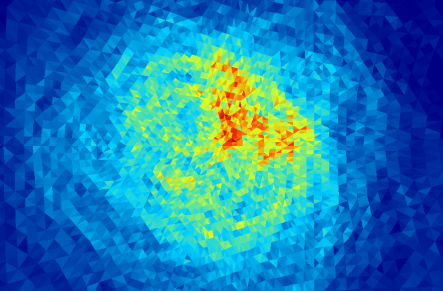
Figure 4: Zoomed image of 10 m-sized L-shaped source

Figure 5: Back-projection Compton imaging of the 10 m-sized L-shaped distributed source with a 1 m $\times$ 6 m vertical section and a 7 m $\times$ 0.5 m horizontal section. The colour scale indicate the number of overlapping back-projected cones. The lower left vertex of the “L” is located in the centre of the image which is projected on to a plane at a distance of 10 m. The horizontal range is 112^∘ and the vertical range is 90^∘. The image corresponds to an acquisition time of 1 second.

V-B Distributed-source results

Reconstructed images of the 100 m-sized and 10 m-sized sources from both the ARDUO and SCoTSS instruments are shown in Figure 3. Here we provide a qualitative comparison of the reconstructed methods applied, with quantitative analyses left for a future publication.

V-B1 100 m-sized L-shaped source

The reconstructed images of the 100 m-sized L-shaped source are shown in Figures 3a, c and e. It is clear from Figure 3a that, using the rate survey method, the performance of both instruments is similar, as would be expected. It is also clear that, using this method, a grid survey of this distributed source with a 10 m line spacing can recover some of the spatial information, but much of the fine detail is absent. Figure 3c indicates how the reconstruction improves when real-time directional information is utilized. In the case of SCoTSS, the image is produced using a back-projection algorithm, with the colour scale indicative of the number of overlapping cones. The neighbouring ARDUO image is formed using the simple direction finding method, with the colour scale indicative of the number of back-projected vectors. It is clear that some finer detail is reconstructed using these methods when compared to the rate survey method, and the performance of both instruments in this setting is roughly comparable, with the SCoTSS imager more accurately reproducing the true shape.

Figure 3e plots the reconstructions using the self-shielding response-function fit method with both instruments. Such analyses require computationally intensive simulations and fitting algorithms and are thus only available in post-processing, after the survey is completed. Noteworthy, however, is that the fine-detail of the distributed source is largely recovered and the performance of both instruments appears comparable.

V-B2 10 m-sized L-shaped source

Reconstruction of a distributed source is challenging for any raster survey method where the grid spacing is similar in size to, or larger than, the source dimensions (see the reconstructions plotted in Figures 3b, d and f). It is clear that the 10 m-sized L-shaped source can be detected and its position is relatively well determined within the 150 m $\times$ 150 m grid. Little fine detail can be recovered with the ARDUO or SCoTSS instruments, when using purely non-imaging directional or survey methods. The finer details of the source are, however, recoverable with the SCoTSS back-projection method (see Figure 5), illustrating the imaging capabilities which motivated the design of the SCoTSS.

VI Concluding remarks and discussion

We have performed a comparative study of the ARDUO and SCoTSS instruments, which are quite similar in terms of their sensor materials, active volume, and electrical components. It is clear that both instruments can localize a point source of emission, with SCoTSS generally faster than ARDUO at achieving a given level of precision. We note that, in self-shielding mode, the performance of both instruments is highly sensitive to the source location. This is particularly true for the SCoTSS imager which, in certain areas of angular phase space can perform poorly, but in others, may out-perform the imaging mode in point source localization. Of course, with SCoTSS, both reconstruction modes can work in tandem and this is a direction we will pursue in the future.

Both instruments have proven capable of imaging a 100 m-sized distributed source in a raster survey, with sharper images obtained in real time when the directional information is included in the reconstruction. Post-acquisition processing methods, such as response-function deconvolution, can further improve the results from both detectors. In a setting such as this - a raster survey with 10 m grid spacing over a 100 m-sized distributed source - our studies show that the ARDUO and SCoTSS instruments perform in a very similar way in head-to-head comparisons in all the methods we tested. We arrive at similar conclusions from our imaging studies performed with a 10 m-sized distributed source, with the notable exception that the SCoTSS instrument can resolve features small in dimension in comparison to the survey parameters, unlike ARDUO. We note, of course, that there are many other relevant deployment scenarios which have not been investigated here. In particular, situations where multiple sources or distributed sources are observed from a stationary position. Imaging capabilities are required in such settings and thus the SCoTSS detector will far outperform purely directional instruments, like ARDUO, in these areas.

References

- [1] Weber, M. 2002, Journal of Luminescence, 100, 35
- [2] Sinclair, L., Saull, P., Hanna, D., et al. 2014, IEEE Transactions on Nuclear Science, 61, 2745
- [3] Sinclair, L. E., Hanna, D. S., MacLeod, A. M. L., & Saull, P. R. B. 2009, IEEE Transactions on Nuclear Science, 56, 1262
- [4] Saull, P. R. B., Sinclair, L. E., Seywerd, H. C. J., et al. 2010, Proc. SPIE, 7665, 76651E-76651E-11
- [5] Compton, A. H. 1923, Physical Review, 21, 483
- [6] Agostinelli, S., Allison, J., Amako, K., et al. 2003, Nuclear Instruments and Methods in Physics Research A, 506, 250
- [7] I. Kawrakow, E. Mainegra-Hing, D. W. O. Rogers, F. Tessier, and B. R. B. Walters, “The EGSnrc Code System, NRC Report PIRS-701,”2011.
- [8] I. Kawrakow, E. Mainegra-Hing, F. Tessier, and B. R. B. Walters, “The EGSnrc C++ class library, NRC Report PIRS-898,” 2011.
- [9] Sinclair, L. E., Marshall, F. A. and Fortin, R. 2015, IEEE Nuclear Science Symposium and Medical Imaging Conference (NSS/MIC), San Diego, CA, pp. 1-4.