Mechanisms for magnetic Field generation in precessing cubes

Abstract

It is shown that flows in precessing cubes develop at certain parameters large axisymmetric components in the velocity field which are large enough to either generate magnetic fields by themselves, or to contribute to the dynamo effect if inertial modes are already excited and acting as a dynamo. This effect disappears at small Ekman numbers. The critical magnetic Reynolds number also increases at low Ekman numbers because of turbulence and small scale structures.

1 Introduction

Precession driven flow is known to lead to magnetic field generation since the first dynamo simulations in precessing spheres (Tilgner, 2005). The mechanisms exciting flows suitable for dynamo action identified in this work were Ekman pumping at the boundaries and triad resonances. The mechanism based on Ekman pumping is superseded at small Ekman numbers by the triad resonances which result from the coupling of inertial waves and which are a bulk instability. Dynamos based on this instability are expected in containers of any shape. They were for instance observed in precessing cubes (Goepfert and Tilgner, 2016).

A laboratory experiment is currently under construction which intends to demonstrate the dynamo effect in precessing sodium filled vessels (Stefani et al., 2015). The construction of the experiment allows for different vessel geometries, but a cylindrical container is the simplest choice and will be realized first. Dynamos in cylinders are little explored as of now. Nore et al. (2011) found dynamos in laminar flows within precessing cylinders. More recently, Giesecke et al. (2018) obtained in the same system dynamos based on axisymmetric flows which resemble very much the kinematic dynamos introduced by Dudley and James (1989) and which inspired the VKS experiment (Monchaux et al., 2007). This discovery motivates us to revisit the problem of the precessing cube and to search for an additional dynamo mechanism in this geometry. The choice of parameters and the issues addressed in the present paper are clearly guided by the laboratory application and not by some astrophysical object.

Section 2 formulates the problem to be simulated. Section 3 describes hydrodynamic processes and the observation of flows analogous to the axisymmetric flows in Giesecke et al. (2018). Section 4 finally deals with dynamo action within these flows.

2 The mathematical model of a precessing cube

A cube of side length $L$ filled with incompressible liquid of density $\rho$ and viscosity $\nu$ rotates with angular frequency $\tilde{\omega}_{D}$ about the $x$-axis and precesses with angular frequency $\tilde{\varOmega}_{P}$. The $x$-axis is part of a Cartesian tripod attached to the cube, whose sides are parallel to $x$, $y$ and $z$-axes. The index $D$ in $\tilde{\omega}_{D}$ stands for diurnal rotation, a term borrowed from the geophysical application (Tilgner, 2015). The precession axis forms the angle $\alpha$ with the $x$-axis.

There are several reasonable options for removing dimensions from the governing equations. Here, we adopt the choice already made in Goepfert and Tilgner (2016) and base the unit of time on the total angular frequency of rotation about the container axis, denoted as $x$-axis, to which both $\tilde{\omega}_{D}$ and $\tilde{\varOmega}_{P}$ contribute. The unit of time is then $1/(\tilde{\omega}_{D}+\tilde{\varOmega}_{P}\cos\alpha)$ and the nondimensional rotation rates $\omega_{D}$ and ${\varOmega}_{P}$ derived form $\tilde{\omega}_{D}$ and $\tilde{\varOmega}_{P}$ are

$$\omega_{D}\,=\, \,\frac{\tilde{\omega}_{D}}{\tilde{\omega}_{D}+\tilde{\varOmega}_{P}\cos\alpha}\,=\,\frac{1}{1+{\varOmega}\cos\alpha}\,,$$ (1)

$${\varOmega}_{P}\,=\, \,\frac{\tilde{\varOmega}_{P}}{\tilde{\omega}_{D}+\tilde{\varOmega}_{P}\cos\alpha}\,=\,\frac{{\varOmega}}{1+{\varOmega}\cos\alpha}$$ (2)

with ${\varOmega}={\varOmega}_{P}/\omega_{D}={\tilde{\varOmega}_{P}}/{\tilde{\omega}_{D}}$. Let hats denote unit vectors. In the $x,y,z-$frame, which we will call the “boundary frame” from now on, the vector of precession $\bm{\varOmega}_{P}$ is given by

$$\bm{\varOmega}_{P}\,=\,{\varOmega}_{P}\cos\alpha~{}\hat{\bm x}+{\varOmega}_{P}~{}\bm p(t)$$ (3)

with

$$\bm p(t)\,=\,\sin\alpha(\cos\omega_{D}t~{}\hat{\bm y}-\sin\omega_{D}t~{}\hat{\bm z})\,.$$ (4)

The equation of motion for the (non-dimensional) velocity $\bm v(\bm r,t)$ as a function of position $\bm r$ and time $t$ and the pressure $\phi(\bm r,t)$ reads in the frame attached to the cube

$$\upartial_{t}\bm v+(\bm v{\bm\cdot}\bm\nabla)\bm v+2(\hat{\bm x}+{\varOmega}_{P}\bm p(t))\times\bm v=\, \,-\bm\nabla\phi+\mathrm{Ek}\nabla^{2}\bm v+{\varOmega}_{P}\omega_{D}(\hat{\bm x}\times\bm p(t))\times\bm r\,,\hskip 22.76219pt$$ (5)

$$\bm\nabla{\bm\cdot}\bm v\,=\, \,0$$ (6)

with an Ekman number $\mathrm{Ek}$ given by

$$\mathrm{Ek}\,=\,\frac{\nu}{(\tilde{\omega}_{D}+\tilde{\varOmega}_{P}\cos\alpha)L^{2}}\,.$$ (7)

It proved useful already in Goepfert and Tilgner (2016) to use a finite difference code implemented on GPUs to simulate precession driven flow in cubes. In order to take full advantage of the special architecture of GPUs, this method avoids the need for any Poisson solver by simulating the flow of a weakly compressible fluid (Tilgner, 2012). If $c$ is the sound speed, this method replaces $\bm\nabla{\bm\cdot}\bm v=0$ with the linearized continuity equation $\upartial_{t}\rho+\bm\nabla{\bm\cdot}\bm v=0$ and the term $-\bm\nabla\phi$ in (5) becomes $-c^{2}\bm\nabla\rho$. The equations actually solved by the finite difference scheme are

$$\upartial_{t}\bm v+(\bm v{\bm\cdot}\bm\nabla)\bm v+2(\hat{\bm x}+{\varOmega}_{P}\bm p(t))\times\bm v\,=\, \,-c^{2}\bm\nabla\rho+\mathrm{Ek}\nabla^{2}\bm v+{\varOmega}_{P}\omega_{D}(\hat{\bm x}\times\bm p(t))\times\bm r\,,\hskip 22.76219pt$$ (8)

$$\upartial_{t}\rho+\bm\nabla{\bm\cdot}\bm v\,=\, \,0\,.$$ (9)

The sound speed $c$ is chosen to keep the Mach number $|\bm v|/c$ below $0.04$ everywhere. In addition, $c$ needs to be large enough so that the time it takes sound waves to travel across the cube is much less than the rotation period, which expressed in the non-dimensional quantities requires $c\gg 2\pi$. In the simulations presented here, $c^{2}=500$. The simulations are started from $\rho=1$ and $|\rho-1|$ stays below $5\times 10^{-4}$ during the course of the computations for this choice of $c^{2}$. The finite value of $c^{2}$ should then have insignificant effects for the purposes of this paper. To confirm this, $c^{2}$ was varied form 500 to 5000 for $\mathrm{Ek}=10^{-4}$ and ${\varOmega}_{P}=-0.018$, and the kinetic energy density $E_{\mathrm{kin}}$, to be defined below, was $1.704\times 10^{-2}\pm 3\times 10^{-5}$ in all cases.

For the kinematic dynamo problem, the induction equation for the magnetic field $\bm B(\bm r,t)$

$$\upartial_{t}\bm B+\bm\nabla\times(\bm B\times\bm v)\,=\,\frac{\mathrm{Ek}}{\mathrm{Pm}}\nabla^{2}\bm B\,,\hskip 42.67912pt\bm\nabla{\bm\cdot}\bm B\,=\,0$$ (10)

is solved together with the equations of motion, where the magnetic Prandtl number $\mathrm{Pm}$ is given by $\mathrm{Pm}={\nu}/{\lambda}$ with $\lambda$ the magnetic diffusivity of the fluid.

Free slip conditions are applied to the velocity field at the boundaries. These enforce that the velocity component normal to a boundary and the normal derivative of the tangential components vanish on the boundary. As in other studies of dynamos in non spherical geometry, we use boundary conditions for the magnetic field which can be expressed locally (Krauze, 2010; Cébron et al., 2012; Giesecke et al., 2015, 2018), namely the pseudo-vacuum boundary conditions which require the tangential components of $\bm B$ to be zero at the boundaries.

The investigated parameter range is essentially the same as in Goepfert and Tilgner (2016) (see table 1) with some points added at large $\mathrm{Ek}$ ($\mathrm{Ek}=10^{-3}$) and large $|{\varOmega}|$. However, the computations were not extended to computationally more demanding parameters than previously, in particular not to small $\mathrm{Ek}$.

$\mathrm{Ek}$	$N$	${\varOmega}_{P}$	$\mathrm{Pm}$
$10^{-3}$	$64$	-0.02…-0.3	1…50
$2.5\cdot 10^{-4}\dots 10^{-4}$	$128$	-0.02 …-0.3	0.1…30
$7.5\cdot 10^{-5}\dots 10^{-5}$	$256$	-0.02…-0.1, -0.16, -0.3	0.1…10

Table 1: Overview of the parameters used in the simulations. $N$ is the number of grid points in each Cartesian direction. The angle $\alpha$ is always set to $\alpha=60^{o}$. Detailed parameters can be deduced from the figures.

3 Hydrodynamics

The main purpose of this section is to show that precessional flow in cubes can contain large fractions of nearly axisymmetric flow, exact axisymmetry being impossible because of the corners and edges of the cube. These axisymmetric flows furthermore have the same topology as some flows studied for their kinematic dynamo properties by Dudley and James (1989). These flows consist of a rotation about a central axis and a meridional circulation built from either one or two tori, designated as $s_{1}t_{1}$ and $s_{2}t_{1}$ flow, respectively, in keeping with the notation introduced in Dudley and James (1989). These flows are sketched in figure 1.

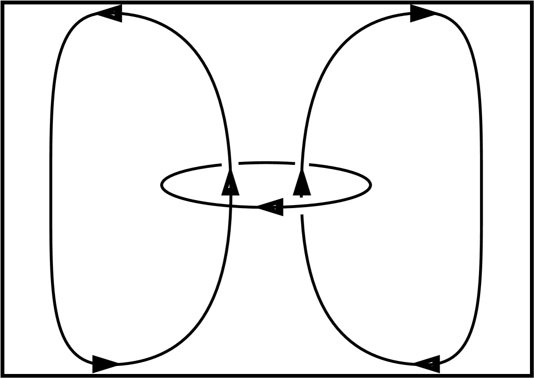
(a) $s_{1}t_{1}$

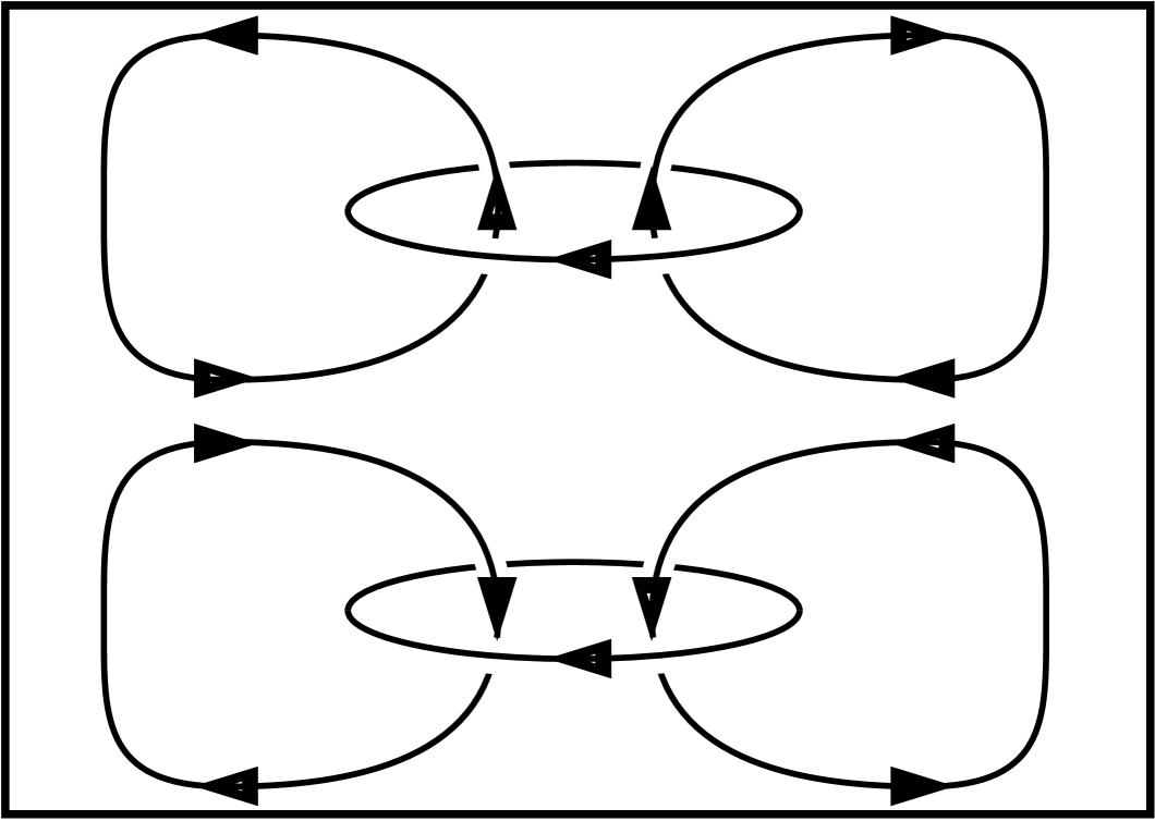
(b) $s_{2}t_{1}$

Figure 1: Sketch of the $s_{1}t_{1}$ (a) and $s_{2}t_{1}$ (b) flows.

In order to construct objective diagnostics for the presence of these flows, consider the following definitions: The energy density of the flow, $E_{\mathrm{kin}}$, is defined as $E_{\mathrm{kin}}={V}^{-1}\big{\langle}\int\frac{1}{2}\bm v^{2}{\mathrm{d}}V\big{\rangle}$ where $\langle\cdots\rangle$ denotes average over time and the integration extends over the entire fluid volume $V$. Note that $V=1$ in our geometry. It will also be useful to consider the part of the velocity field $\bm v_{a}$ which is antisymmetric with respect to reflection at the origin,

$$\bm v_{a}\,=\,\tfrac{1}{2}\bigl{(}\bm v(\bm r)+\bm v(-\bm r)\bigr{)}$$ (11)

and its energy

$$E_{a}\,=\,\frac{1}{V}\biggl{\langle}\,\int\tfrac{1}{2}\bm v_{a}^{2}\,{\mathrm{d}}V\biggr{\rangle}\,.$$ (12)

These quantities were used in the past for detecting instability. In the present context, they are also of interest because $E_{a}=0$ for the $s_{2}t_{1}$ flow, whereas $E_{a}\neq 0$ for the $s_{1}t_{1}$ flow because of its meridional components. It is however more intuitive to distinguish the $s_{1}t_{1}$ and $s_{2}t_{1}$ flows thanks to a mirror symmetry. Let us define the velocity field $\bm v_{e}$ which is the part of $\bm v$ which is mirror symmetric with respect to the plane perpendicular to the rotation axis $x$ and which divides the cube in two equal halves:

$$v_{es}(s,\varphi,x)\,=\, \,\tfrac{1}{2}\bigl{(}v_{s}(s,\varphi,x)+v_{s}(s,\varphi,-x)\bigr{)}\,,$$

$$v_{e\varphi}(s,\varphi,x)\,=\, \,\tfrac{1}{2}\bigl{(}v_{\varphi}(s,\varphi,x)+v_{\varphi}(s,\varphi,-x)\bigr{)}\,,$$

$$v_{ex}(s,\varphi,x)\,=\, \,\tfrac{1}{2}\bigl{(}v_{x}(s,\varphi,x)-v_{x}(s,\varphi,-x)\bigr{)}\,.$$

where $(s,\varphi,x)$ are cylindrical coordinates with the $x$-axis as distinguished axis. The index $e$ stands for equatorially symmetric because of the obvious analogy with equatorially symmetric flows in spheres. $\bm v_{e}=\bm v$ for the $s_{2}t_{1}$ flow, whereas the $s_{1}t_{1}$ flow has again mixed symmetry.

We next have to separate the axisymmetric components from the others. We obtain the axisymmetric contributions to the velocity components $v_{s}$, $v_{\varphi}$, $v_{x}$ from the integral

$$v_{x0}(s,x)\,=\,\frac{1}{2\pi}\int_{0}^{2\pi}v_{x}(s,\varphi,x)\,{\mathrm{d}}\varphi\bigg{/}\left(\frac{1}{2\pi}\int_{0}^{2\pi}I(s,\varphi,x)\,{\mathrm{d}}\varphi\right)$$ (13)

and likewise for $v_{s0}$, $v_{\varphi 0}$ and the axisymmetric and equatorially symmetric components $v_{ex0}$, $v_{es0}$, $v_{e\varphi 0}$. The arguments of all these quantities have to span the intervals $0\leq x\leq 1$ and $0\leq s\leq\sqrt{2}/2$. The integration in (13) extends over regions partly outside the cube for $1/2<s\leq\sqrt{2}/2$. The average in (13) is intended to be an average over the cube, so that $v_{x}$ is set to zero outside the cube, and the function $I(s,\varphi,x)$ is 1 within the cube and zero outside. The azimuthally averaged velocities are finally transformed into energies as for example in

$$E_{x0}\,=\,\frac{1}{V}\biggl{\langle}\,\int\tfrac{1}{2}v_{x0}^{2}\,{\mathrm{d}}V\biggr{\rangle}$$ (14)

and similarly for $E_{s0}$, $E_{\varphi 0}$ and $E_{ex0}$, $E_{es0}$, $E_{e\varphi 0}$.

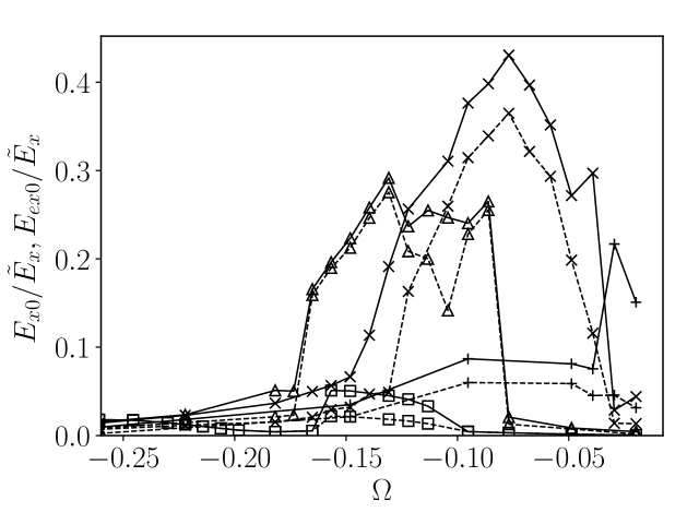
(a)

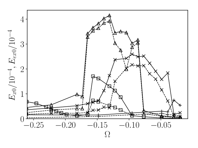
(b)

(c) (a) $E_{x0}/\tilde{E}_{x}$ as a function of ${\varOmega}$ for $\mathrm{Ek}=1.0\cdot 10^{-3}$ ($\square$),$\mathrm{Ek}=2.5\cdot 10^{-4}$ ($\triangle$), $\mathrm{Ek}=1.0\cdot 10^{-4}$ ($\times$) and $\mathrm{Ek}=1.0\cdot 10^{-5}$ ($+$). The continuous lines connect points for $E_{x0}/\tilde{E}_{x}$, and the dashed lines are for $E_{ex0}/\tilde{E}_{x}$. (b) $E_{x0}$ as a function of ${\varOmega}$ with the same symbols as in (a).

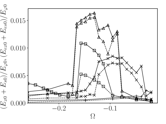
(d)

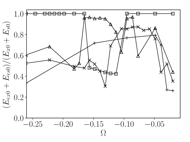
(e)

(f) (a) $(E_{x0}+E_{s0})/E_{\varphi 0}$ and $(E_{ex0}+E_{es0})/E_{\varphi 0}$ as a function of ${\varOmega}$ for $\mathrm{Ek}=1.0\cdot 10^{-3}$ ($\square$),$\mathrm{Ek}=2.5\cdot 10^{-4}$ ($\triangle$), $\mathrm{Ek}=1.0\cdot 10^{-4}$ ($\times$) and $\mathrm{Ek}=1.0\cdot 10^{-5}$ ($+$). The continuous lines connect points for $(E_{x0}+E_{s0})/E_{\varphi 0}$, and the dashed lines are for $(E_{ex0}+E_{es0})/E_{\varphi 0}$. (b) $(E_{ex0}+E_{es0})/(E_{x0}+E_{s0})$ as a function of ${\varOmega}$ with the same symbols as in (a).

Yet another quantity appears in figure 3, which is $\tilde{E}_{x}$, the energy contained in the non-axisymmetric components of $v_{x}$:

$$\tilde{E}_{x}\,=\,\frac{1}{V}\biggl{\langle}\,\int\tfrac{1}{2}(v_{x}-v_{x0})^{2}\,{\mathrm{d}}V\biggr{\rangle}\,.$$ (15)

Figure 3(a) plots $E_{x0}/\tilde{E}_{x}$ as a function of ${\varOmega}$ for different $\mathrm{Ek}$. This quantity detects a dramatic increase of the axisymmetric components at some ${\varOmega}$. This increase is not spread equally among the velocity components, as revealed by figure 3(a). This figure shows $(E_{x0}+E_{s0})/E_{\varphi 0}$ as a function of ${\varOmega}$ and thus compares axisymmetric meridional and azimuthal components. Large values in figures 3 and 3(a) correlate with each other, which means that if a large axisymmetric component appears at some ${\varOmega}$, it appears because the axisymmetric meridional components have increased.

Precession forces a basic flow in the container frame which is approximately a solid body rotation about an axis other than the rotation axis of the container. This flow thus contains already through direct forcing and without intervening instability non axisymmetric components which contribute to $\tilde{E}_{x}$, and axisymmetric components which contribute to $E_{\varphi 0}$. Figures 3(a) and 3(a) show broadly the same variation because $\tilde{E}_{x}$ and $E_{\varphi 0}$ both are dominated by the basic flow which exists at all ${\varOmega}$, whereas $E_{s0}$ and $E_{x0}$ have significant magnitude only in certain intervals of ${\varOmega}$. For comparison, figure 3(b) shows $E_{x0}$ without normalization with $\tilde{E}_{x}$ exhibits rapid variations as a function of ${\varOmega}$ at the same ${\varOmega}$ as figure 3(a).

Figure 3(a) also shows $(E_{ex0}+E_{es0})/E_{\varphi 0}$. This ratio exactly coincides with $(E_{x0}+E_{s0})/E_{\varphi 0}$ if the axisymmetric part of the flow is purely of the $s_{2}t_{1}$ type. If the two ratios differ, there is a contribution to the axisymmetric flow by the opposite symmetry, whose simplest representative is the $s_{1}t_{1}$ flow. There is generally some admixture of both symmetries. For a quantitative measure, figure 3(b) plots $(E_{ex0}+E_{es0})/(E_{x0}+E_{s0})$. This ratio is 1 in an $s_{2}t_{1}$ flow and 0 in a pure $s_{1}t_{1}$ flow. Figure 3(b) shows that the $s_{2}t_{1}$ flow clearly dominates the axisymmetric flow at some parameters, while it contributes less than one half of the axisymmetric meridional flow at other parameters.

Visualizations such as in figure 3 confirm that the sketches in figure 1 qualitatively represent the actual flows. Figure 3 shows contour plots of the equatorially antisymmetric and symmetric part of $v_{x0}$ at $\mathrm{Ek}=10^{-4}$ and ${\varOmega}=-0.04$. One recognizes the $s_{2}t_{1}$ and $s_{1}t_{1}$ patterns but one also notices that $v_{x0}$ has a single sign for $0\leq s\lesssim 1/2$ in each half of the cube, so that the return flows must mostly occur near the edges of the cube in the region $1/2\leq s\leq\sqrt{2}/2$.

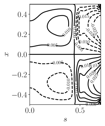
(g)

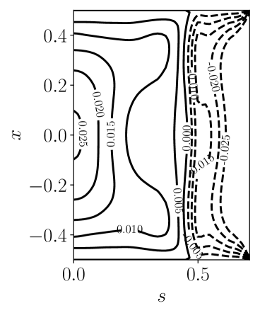
(h)

(i) Contour plots of (a) $v_{ex0}$ and (b) $v_{x0}-v_{ex0}$, at $\mathrm{Ek}=10^{-4}$ and ${\varOmega}=-0.04$

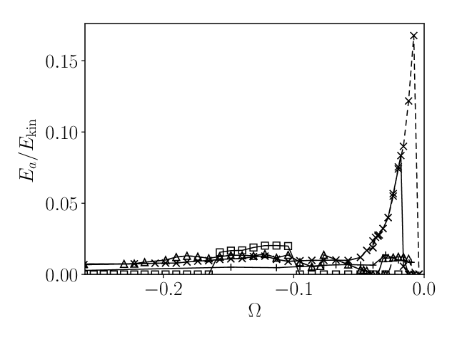
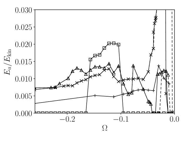
Figure 2: $E_{a}/E_{\mathrm{kin}}$ as a function of ${\varOmega}$ for $\mathrm{Ek}=1.0\cdot 10^{-3}$ ($\square$), $\mathrm{Ek}=2.5\cdot 10^{-4}$ ($\triangle$), $\mathrm{Ek}=1.0\cdot 10^{-4}$ ($\times$) and $\mathrm{Ek}=1.0\cdot 10^{-5}$ ($+$). The dashed line is followed when decreasing $|{\varOmega}|$, the continuous line is obtained in going in the opposite direction. The right panel shows the same data as the left panel on a different scale.

The antisymmetric components $\bm v_{a}$ can be excited only via an instability. Their energy $E_{a}$, defined in (12), is therefore a convenient indicator for the presence of instability. Figure 2 shows $E_{a}/E_{\mathrm{kin}}$ for comparison with figures 3 and 3. It is seen that for $\mathrm{Ek}=10^{-3}$, the interval of ${\varOmega}$ in which $E_{a}/E_{\mathrm{kin}}\neq 0$ coincides with the interval in which significant axisymmetric components are present in the meridional flow. In fact, at this $\mathrm{Ek}$, there is no other instability than the one leading to the $s_{2}t_{1}$ and $s_{1}t_{1}$ flows. At the other $\mathrm{Ek}$, however, the flow first becomes unstable through triad resonances (Goepfert and Tilgner, 2016) and the $s_{2}t_{1}$ and $s_{1}t_{1}$ flows exist side by side with inertial modes.

4 Kinematic dynamos

There are several possible definitions of the magnetic Reynolds number which are potentially of interest and which differ in the velocity on which they are based. The definition which is most directly related to the parameters of an experiment is the magnetic Reynolds number computed from the rotational velocity of the container about its axis, $\mathrm{Rm}_{\mathrm{rot}}$, given by

$$\mathrm{Rm}_{\mathrm{rot}}\,=\,\mathrm{Pm}/(2\mathrm{Ek})\,.$$ (16)

Structural stability and the available motors naturally set a limit on the largest $\mathrm{Rm}_{\mathrm{rot}}$ achievable in an experiment, which happens to be 1420 in the Dresden experiment (Stefani et al., 2012, 2015).

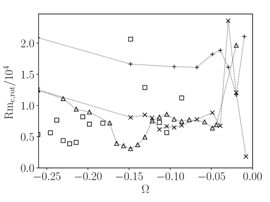
Figure 3: $\mathrm{Rm}_{\mathrm{c,rot}}$ as a function of ${\varOmega}$ for $\mathrm{Ek}=1.0\cdot 10^{-3}$ ($\square$), $\mathrm{Ek}=2.5\cdot 10^{-4}$ ($\triangle$), $\mathrm{Ek}=1.0\cdot 10^{-4}$ ($\times$) and $\mathrm{Ek}=1.0\cdot 10^{-5}$ ($+$).

The critical value of this magnetic Reynolds number, $\mathrm{Rm}_{\mathrm{c,rot}}$, is shown for the various simulations in figure 3. For all $\mathrm{Ek}<10^{-3}$, a triad resonance occurs. Inertial modes in triads are known to be able to generate magnetic fields, so that these triads are responsible for a baseline in this figure and also for some of the salient variations. For instance, the best dynamo in figure 3 is realized at $\mathrm{Ek}=10^{-4}$ and ${\varOmega}=-0.008$, which is within a hysteresis loop so that this flow must be accessed by lowering $|{\varOmega}|$ from higher values (see figure 2). The $\mathrm{Rm}_{\mathrm{c,rot}}$ is then 1820. At these parameters, the energy in the antisymmetric and hence unstable modes is exceptionally large as can be seen in figure 2, whereas the axisymmetric energy stays small according to figures 3 and 3, so that this dynamo is driven by a triad.

There are other notable variations in $\mathrm{Rm}_{\mathrm{c,rot}}$ in figure 3 which correlate with axisymmetric flow components. Figures 3(a) and 3(a) tell us whether an axisymmetric flow of large amplitude comes on top of the inertial modes, and we can deduce from figure 3(b) whether this flow is mostly of the $s_{2}t_{1}$ structure or whether there are large contributions by the $s_{1}t_{1}$ flow. The recognizable dips in the curve representing $\mathrm{Rm}_{\mathrm{c,rot}}$ in figure 3 occur in intervals of ${\varOmega}$ in which an $s_{2}t_{1}$ flow of significant amplitude is present (for example for $\mathrm{Ek}=2.5\times 10^{-4}$ around ${\varOmega}=-0.15$). If on the contrary there is a large contribution by a flow of the $s_{1}t_{1}$ type (at $\mathrm{Ek}=10^{-3}$ around ${\varOmega}=-0.15$), the dynamo worsens. The axisymmetric flows thus have an effect on magnetic field generation, but they are not necessarily helpful. In the available examples, the $s_{2}t_{1}$ component tends to lower $\mathrm{Rm}_{\mathrm{c,rot}}$ whereas $s_{1}t_{1}$ acts in the opposite direction.

It is known from optimization studies done in connection with the VKS experiment (Ravelet et al., 2005) that axisymmetric flows of the type studied by Dudley and James (1989) are most effective at generating magnetic fields if their poloidal and toroidal energies are comparable. The flows studied here all have $(E_{x0}+E_{s0})/E_{\varphi 0}<0.016$ (see figure 3(a)) and must be inefficient according to this criterion. Figure 4 collects all the dynamos with a significant $s_{2}t_{1}$ flow. The critical magnetic Reynolds number is on the order of several thousands as opposed to one hundred for the optimized flows in Ravelet et al. (2005), and the critical magnetic Reynolds number decreases with increasing $(E_{x0}+E_{s0})/E_{\varphi 0}$ at small $(E_{x0}+E_{s0})/E_{\varphi 0}$.

While the $s_{2}t_{1}$ flow helps dynamo action, its presence does not lower the critical magnetic Reynolds number in our examples to a value accessible in the Dresden experiment.

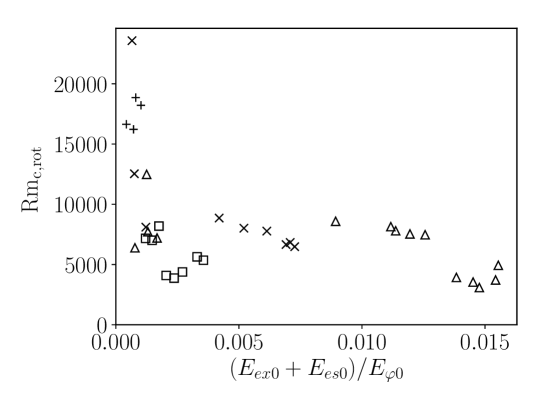
Figure 4: $\mathrm{Rm}_{\mathrm{c,rot}}$ as a function of $(E_{x0}+E_{s0})/E_{\varphi 0}$ for dynamos in flows with $(E_{ex0}+E_{es0})>\frac{1}{2}(E_{x0}+E_{s0})$, which selects flows dominated by the $s_{2}t_{1}$ flow in their axisymmetric components. The different markers stand for $\mathrm{Ek}=1.0\cdot 10^{-3}$ ($\square$), $\mathrm{Ek}=2.5\cdot 10^{-4}$ ($\triangle$), $\mathrm{Ek}=1.0\cdot 10^{-4}$ ($\times$) and $\mathrm{Ek}=1.0\cdot 10^{-5}$ ($+$).

Simulations of both astrophysical objects and experiments generally have the problem that they cannot simulate the small Ekman numbers which are of interest. The Dresden experiment for instance can be operated at $\mathrm{Ek}$ as low as $10^{-8}$, whereas all our simulations are at $\mathrm{Ek}\geq 10^{-5}$. The behavior at small $\mathrm{Ek}$ has to be deduced from extrapolations. Ideally, the extrapolation is based on theory and physical understanding. In order to safely extrapolate the dynamo properties of the $s_{2}t_{1}$ flow, we would need to know how it is excited, and whether it will persist at small $\mathrm{Ek}$. The mechanism exciting this flow is not elucidated. The pattern of the $s_{2}t_{1}$ flow is compatible with a centrifugal instability, as proposed by Giesecke et al. (2018). Whatever the true mechanism may be, it seems to become inoperative at low $\mathrm{Ek}$. As figure 5 shows, $E_{x0}/\tilde{E}_{x}\rightarrow 0$ as $\mathrm{Ek}\rightarrow 0$ at any fixed ${\varOmega}$, so that we have to expect the beneficial effects of the $s_{2}t_{1}$ flow for the dynamo to disappear at small $\mathrm{Ek}$. This is part of the reason why critical magnetic Reynolds numbers generally increase with decreasing $\mathrm{Ek}$, as shown in figure 6. However, also the dynamos among our simulations operating with triadic resonances deteriorate with decreasing $\mathrm{Ek}$, so that there must be yet another reason for this behavior.

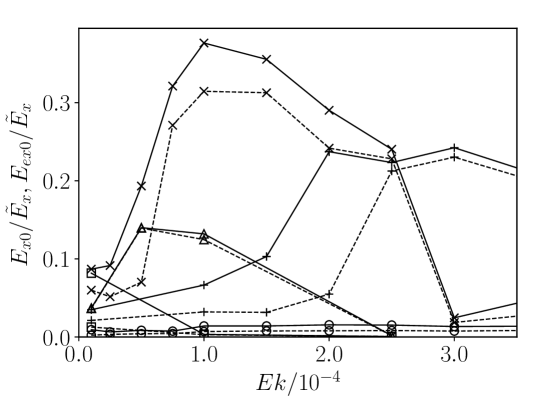
Figure 5: $E_{x0}/\tilde{E}_{x}$ as a function of $\mathrm{Ek}$ for ${\varOmega}=-0.1$ ($\times$), ${\varOmega}=-0.15$ ($+$) and ${\varOmega}=-0.26$ ($\circ$). The continuous lines connect points for $E_{x0}/\tilde{E}_{x}$, and the dashed lines are for $E_{ex0}/\tilde{E}_{x}$.

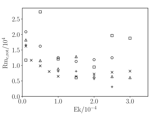
Figure 6: $\mathrm{Rm}_{\mathrm{c,rot}}$ as a function of $\mathrm{Ek}$ for ${\varOmega}=-0.02$ ($\square$), ${\varOmega}=-0.05$ ($\triangle$), ${\varOmega}=-0.1$ ($\times$), ${\varOmega}=-0.15$ ($+$) and ${\varOmega}=-0.26$ ($\circ$).

Another contribution to this effect may come from increasing turbulence and the appearance of small scales at small $\mathrm{Ek}$. Let us use a dissipation length scale $L_{D}$ as diagnostics for the presence of small scale structures. The dissipation $D$ is given by

$$D\,=\,\mathrm{Ek}\,\frac{1}{V}\biggl{\langle}\,\int\sum_{ij}(\upartial_{i}v_{j})^{2}\,{\mathrm{d}}V\biggr{\rangle}\,=\,\frac{1}{V}\,\biggl{\langle}\,\int\bm v{\bm\cdot}\bigl{(}{\varOmega}_{P}\omega_{D}(\hat{\bm x}\times\bm p(t))\times\bm r\bigr{)}\,{\mathrm{d}}V\biggr{\rangle}\,.$$ (17)

The last equation results from taking the scalar product of (5) with $\bm v$, integrating over space and averaging over time. While both expressions for $D$ are identical analytically, the first expression incurs the larger numerical error because it depends on derivatives, so that the second expression was always used to extract $D$ from the numerical results. Finally, the dissipation length is defined as

$$L_{D}\,=\,\sqrt{E_{\mathrm{kin}}/D}\,.$$ (18)

As expected, $L_{D}$ is approximately constant in the laminar flows and decreases with decreasing $\mathrm{Ek}$ at small $\mathrm{Ek}$ (see figure 7). The decrease in $L_{D}$ correlates with the increase of $\mathrm{Rm}_{\mathrm{c,rot}}$ in figure 6. To make this clear, figure 8 plots $\mathrm{Rm}_{\mathrm{c,rot}}$ directly as function of $L_{D}$. Studies in dependence of $\mathrm{Ek}$ in precessing cubes are complicated because the flow may undergo transitions between different states as $\mathrm{Ek}$ is varied (Goepfert and Tilgner, 2016), for example between different triad resonances, or a triad resonance and a single vortex state, or a significant axisymmetric component may come and go. This is particularly true of the points with ${\varOmega}=-0.02$ which are therefore not shown in figure 8. At least at the precession rates included in figure 8, $\mathrm{Rm}_{\mathrm{c,rot}}$ varies as a function of $L_{D}$ for fixed ${\varOmega}$ on lines parallel to each other, suggesting that the eddy diffusivity introduced by turbulence is increasing the critical magnetic Reynolds number.

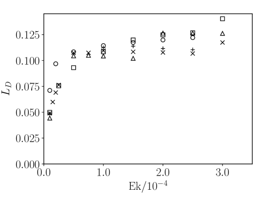
Figure 7: $L_{D}$ as a function of $\mathrm{Ek}$ for ${\varOmega}=-0.02$ ($\square$), ${\varOmega}=-0.05$ ($\triangle$), ${\varOmega}=-0.1$ ($\times$), ${\varOmega}=-0.15$ ($+$) and ${\varOmega}=-0.26$ ($\circ$).

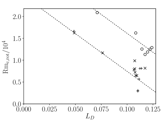
Figure 8: $\mathrm{Rm}_{\mathrm{c,rot}}$ as a function of $L_{D}$. The different markers stand for ${\varOmega}=-0.1$ ($\times$), ${\varOmega}=-0.15$ ($+$) and ${\varOmega}=-0.26$ ($\circ$). The upper dashed lines guide the eye through the points for ${\varOmega}=-0.26$ and the other through all remaining points.

5 Conclusion

Several mechanisms enabling precession driven flows to act as dynamos have been identified in the past. Ekman pumping at the boundaries and triad resonances were the first to be observed (Tilgner, 2005). Dynamos in long slender vortices which form at low Ekman numbers were found later (Goepfert and Tilgner, 2016). Recently (Giesecke et al., 2018), it was shown that for certain parameters, the flow in precessing cylinders resembles the $s_{2}t_{1}$ flow studied by Dudley and James (1989) as kinematic dynamo in a sphere. The present work confirms the appearance of this $s_{2}t_{1}$ flow to be a common feature in precessing flows. The $s_{2}t_{1}$ flow helps in generating magnetic fields, although not to the extent that the results from precessing cubes allow one to propose parameters at which the Dresden experiment should act as a dynamo. We also find $s_{1}t_{1}$ flows in the cube. There is no theory yet as to what drives these flows. It is therefore not possible to safely extrapolate the numerical results to small Ekman numbers. A purely empirical extrapolation is difficult because the flow transits between different states as the Ekman number is lowered at fixed precession rate. Generally, however, the critical magnetic Reynolds number increases in our sinulations with decreasing Ekman number at low Ekman numbers. This increase occurs in parallel to the appearance of turbulence and small scales in the flow. In addition, the strong axisymmetric flow components disappear at small Ekman numbers.

References

- (1)
- (2)
- Cébron et al. (2012) Cébron, D., Le Bars, M., Maubert, P. and Le Gal, P., Magnetohydrodynamic simulations of the elliptical instability in triaxial ellipsoids. Geophys. Astrophys. Fluid Dyn., 2012, 106, 524–546.
- Dudley and James (1989) Dudley, M. and James, R., Time dependent kinematic dynamos with stationary flows. Proc. R. Soc. Lond. A, 1989, 425, 407–429.
- Giesecke et al. (2015) Giesecke, A., Albrecht, T., Gundrum, T., Herault, J. and Stefani, F., Triadic resonances in non-linear simulations of fluid flow in a precessing cylinder. New J. Phys., 2015, 17, 113044.
- Giesecke et al. (2018) Giesecke, A., Vogt, T., Gundrum, T. and Stefani, F., The non-linear large scale flow in a precessing cylinder and its ability to drive dynamo action. Phys. Rev. Lett., 2018, 120, 024502.
- Goepfert and Tilgner (2016) Goepfert, O. and Tilgner, A., Dynamos in precessing cubes. New Journal of Physics, 2016, 18, 103019.
- Krauze (2010) Krauze, A., Numerical modeling of the magnetic field generation in a precessing cube with a conducting melt. Magnetohydrodynamics, 2010, 46, 271–280.
- Monchaux et al. (2007) Monchaux, R., Berhanu, M., Bourgoin, M., Moulin, M., Odier, P., Pinton, J.F., Volk, R., Fauve, S., Mordant, N., Pétrélis, F., Chiffaudel, A., Daviaud, F., Dubrulle, B., Gasquet, C., Marié, L. and Ravelet, F., Generation of a magnetic field by dynamo action in a turbulent flow of liquid sodium. Phys. Rev. Lett., 2007, 98, 044502.
- Nore et al. (2011) Nore, C., Léorat, J., Guermond, J.L. and Luddens, F., Nonlinear dynamo excitation in a precessing cylindrical container. Phys. Rev. E, 2011, 84, 016317.
- Ravelet et al. (2005) Ravelet, F., Chiffaudel, A., Daviaud, F. and Léorat, J., Toward an experimental von Kármán dynamo: Numerical studies for an optimized design. Phys. Fluids, 2005, 17, 117104.
- Stefani et al. (2015) Stefani, F., Albrecht, T., Gerbeth, G., Giesecke, A., Gundrum, T., Herault, J., Nore, C. and Steglich, C., Towards a precession driven dynamo experiment. Magnetohydrodynamics, 2015, 51, 275–284.
- Stefani et al. (2012) Stefani, F., Eckert, S., Gerbeth, G., Giesecke, A., Gundrum, T., Steglich, C., Weier, T. and Wustmann, B., DRESDYN - A new facility for MHD experiments with liquid sodium. Magnetohydrodynamics, 2012, 48, 103–113.
- Tilgner (2005) Tilgner, A., Precession driven dynamos. Phys. Fluids, 2005, 17, 034104.
- Tilgner (2012) Tilgner, A., Transitions in rapidly rotating convection dynamos. Phys. Rev. Lett., 2012, 109, 248501.
- Tilgner (2015) Tilgner, A., Rotational Dynamics of the core; in Treatise on Geophysics, 2nd edition, edited by G. Schubert, Vol. 8, 2015, pp. 183–212.