Domain wall dynamics for an in-plane magnetized thin film with large perpendicular hard axis anisotropy including Dzyaloshinskii-Moriya interaction.

Abstract

We consider a thin ferromagnetic layer to which an external field or a current are applied along an in plane easy axis. The perpendicular hard axis anisotropy constant is large so that the out of plane magnetization component is smaller than the in plane components. A perturbation approach is used to obtain the profile and velocity of the moving domain wall. The dynamics of the in plane components of the magnetization is governed by a reaction diffusion equation which determines the speed of the profile. We find a simple analytic expression for the out of plane magnetization showing a symmetric distortion due to the motion in addition to the asymmetric component due to the Dzyaloshinskii–Moriya interaction. The results obtained complement previous studies in which either the Dzyalozhinskii vector or the out of plane hard axis anisotropy were assumed small. In the regime studied the Walker breakdown is not observed but the reaction diffusion dynamics predicts a slowing down of the domain wall for sufficiently large magnetic field. The transition point depends on the applied field, saturation magnetization and easy axis anisotropy.

I Introduction

Magnetic domain wall propagation is an active area of research both as an interesting physical phenomenon as well as for its possible applications in logic devices, magnetic memory elements and others Allwood et al. (2005); Stamps et al. (2014). In the micromagnetic approximation the dynamics of the magnetization is governed by the Landau Lifshitz Gilbert (LLG) equation Landau and Lifshitz (1935); Gilbert (1956), which cannot be solved except in special cases. The classic Walker solution takes into account exchange interaction, interactions modeled as effective anisotropies and studies a domain wall (DW) driven by an external magnetic field. The inclusion of additional physical interactions does not allow for simple analytical solutions. Of particular interest and a subject of current research is the asymmetric Dzyalozhinskii–Moriya interaction (DMI) Dzyaloshinsky (1958); Moriya (1960) which leads to new types of DW inducing a rotation of the magnetization and stabilizing chiral DWs. Most studies including DMI address the case of interfacial DMI in perpendicularly magnetized thin films as it increases significantly both the DW speed and Walker field Thiaville et al. (2012); Emori et al. (2013).

The role of DMI in in-plane magnetized thin layers has received less attention, recent experimental work Thevenard et al. (2017) finds significant differences with out of plane magnetized films. This configuration, including bulk DMI, was studied analytically in Tretiakov and Abanov (2010); Kravchuk (2014); Wang et al. (2015); Zhuo and Sun (2016) using the method of collective coordinates. In Tretiakov and Abanov (2010) as in Zhuo and Sun (2016) the starting point for the application of the collective coordinates method is a profile that neglects the perpendicular hard axis anisotropy which is included as a small perturbation. A similar approach is taken in Wang et al. (2015) where magnon driven DW motion is studied. A different approach is taken in Kravchuk (2014) where the DMI is considered as a small perturbation . A fairly complex analytic form for the perturbation to the static profile due to DMI is found in Kravchuk (2014) and a linear analysis of this correction to the profile at the center of the domain wall provides the ansatz for the application of the collective coordinate method. The numerical and analytic results shown in Tretiakov and Abanov (2010); Kravchuk (2014); Wang et al. (2015); Zhuo and Sun (2016) show an asymmetric deformation of the static DW profile due to DMI. The effect on the speed of different orientations of the easy axis relative to the Dzyaloshinski vector are studied in Wieser (2016).

Here we study a different case. We are interested in the case where the effective hard axis anisotropy $K_{d}$ is much larger than the in plane easy axis effective anisotropy $K_{u}$ and at the same time all the components of the effective field remain of comparable magnitude. These two requirements dictate the scalings needed to perform an asymptotic expansion of the LLG equation using as a small parameter the ratio of the easy and hard axis anisotropies $K_{u}/K_{d}$. The numerical and analytical work of Wieser et al. (2010); Wang et al. (2012); Hu and Wang (2013); Wang and Wang (2014) shows that this regime leads to behavior which differs substantially from the the case where $K_{d}$ is of the same order as $K_{u}$. Materials with a large disparity of anisotropies were studied in Thevenard et al. (2012) where suitably prepared samples of (Ga,Mn)(As,P) with a wide range of effective anisotropies are considered.. In particular, sample A3 achieves the ratio $K_{u}/K_{d}=0.005$. The speed of propagation of the domain wall in this sample is in qualitative agreement with the numerical results cited above and cannot be explained by the Walker solution. Instability of the Walker solution has been shown analytically in the same scenario Hu and Wang (2013). The presence of the small quantity $K_{u}/K_{d}$ enables one to perform an asymptotic expansion of the LLG equation to obtain the leading order dynamical behavior in this regime. Perturbative approaches to reduce the LLG dynamics to simpler equations with different assumptions have been employed in Mikeska (1978); Garcia-Cervera and E (2001); Bazaliy (2007); Goussev et al. (2016); Lund et al. (2016) among others. We find that the dynamics of the in-plane components is governed by a reaction diffusion equation and that the out of plane component is determined by the in-plane profile and depends on the applied current and magnetic field in addition to the DMI interaction. The in- plane components of the magnetization for a tail to tail (TT) configuration are given by the usual profile

$$m_{x}^{TT}=\tanh\left(\frac{x-vt}{\Delta}\right),\qquad m_{y}^{TT}=\text{sech}\left(\frac{x-vt}{\Delta}\right),$$ (1)

where the width is given in terms of the exchange constant $C_{\text{ex}}$ and the easy axis anisotropy $K_{u}$ by $\Delta=\sqrt{C_{\text{ex}}/(2K_{u})}$.

For an external current $u$ and magnetic field $H_{a}$ applied along the easy $x$ axis, the out of plane magnetization is found to be

$$m_{z}^{TT}=\frac{M_{s}}{2|\gamma|\Delta K_{d}}\text{sech}\left(\frac{x-vt}{\Delta}\right)\left[u-v+\frac{2D|\gamma|}{M_{s}}\tanh\left(\frac{x-vt}{\Delta}\right)\right],$$ (2)

where the speed $v$ for the TT domain wall in the limit studied is given by

$$v=-\mu_{0}|\gamma|\frac{\Delta H_{a}}{\alpha}+\frac{\beta u}{\alpha}$$

where $D$, $H_{a}$ and $u$ are the Dzyaloshinski constant and the applied magnetic field and current respectively. The quantities $\alpha$, $\beta$ and $\gamma$ are the Gilbert damping, the nonadiabatic Thiaville et al. (2005) parameter and the electron gyromagnetic ratio. An equivalent expression holds for a head to head (HH) domain wall. The static profile is in qualitative agreement with the numerical results reported in Wang et al. (2015) and with the analytic solution for small DMI obtained in Kravchuk (2014). The explicit expression for the out of plane magnetization showing the effect of the DMI and applied field and current on the profile for large easy plane anisotropy, Eq.(2), has not been reported elsewhere to the best of our knowledge. The main effect of the motion is to change the symmetry property $m_{z}(-x)=-m_{z}(x)$ of the static solution losing all symmetry as it moves. The above solution is found from the leading order expansion of the LLG equation.

The dynamics in the limit studied is different from that found for the thin film with small perpendicular anisotropy or with small DMI Tretiakov and Abanov (2010); Kravchuk (2014). The reaction diffusion equation which governs the in-plane dynamics shows that for sufficiently large external field an initial perturbation will not evolve into this exact analytic solution but it will evolve into a Kolmogorov-Petrovskii-Piscounov (KPP) Kolmogorov et al. (1937) domain wall moving with slower speed but qualitatively similar profile. The transition point and this slower speed are given below. Previous numerical work has shown a slowdown of the domain wall before encountering the Walker field Wieser et al. (2010); Wang et al. (2012); Wang and Wang (2014) for thin films with very large hard axis anisotropy. They attribute the slow down of the domain wall to spin wave emission. The analytical results found in this work show similar qualitative behavior as that found numerically. In the present approach we are able to obtain the envelope of the domain wall, therefore identification of the slow down by spin wave emission with a transition from pushed to pulled fronts is not possible without further work.

In Section II we state the problem, in Section III we perform an asymptotic analysis and solve the resulting equation and in Section IV we summarize the results.

II Statement of the problem

We consider a thin narrow film in the $(x,y)$ plane, with the easy axis $x$ along its length and an effective hard axis perpendicular to the thin film plane. A constant external field and current are applied along the easy axis $\vec{H}_{a}=H_{a}\hat{x}$, $\vec{u}=u\hat{x}$. Wang et al. (2015)

The material has magnetization $\vec{M}=M_{s}\vec{m}$ where $M_{s}$ is the saturation magnetization and $\vec{m}=(m_{1},m_{2},m_{3})$ is the unit vector along the direction of magnetization. The dynamic evolution of the magnetization is governed by the LLG equation, including the current

$$\frac{\partial\vec{m}}{\partial t}=-\gamma_{0}\vec{m}\times\vec{H}_{\mbox{{\tiny eff}}}+\alpha\vec{m}\times\frac{\partial\vec{m}}{\partial t}-(\vec{u}\cdot\vec{\nabla})\vec{m}+\beta\vec{m}\times(\vec{u}\cdot\vec{\nabla})\vec{m}$$ (3)

where $\vec{H}_{\mbox{{\tiny eff}}}$ is the effective magnetic field, $\gamma_{0}=|\gamma|\mu_{0}$, $\gamma$ is the gyromagnetic ratio of the electron, $\mu_{0}$ is the magnetic permeability of vacuum. The constant $\alpha>0$ is the dimensionless phenomenological Gilbert damping coefficient. The vector $u$ is proportional to the current density $j_{e}$ and has units of velocity. The dimensionless constant $\beta$ is the non adiabaticity parameter.

The effective magnetic field is given by Wieser et al. (2010); Wang et al. (2012); Hu and Wang (2013); Wang and Wang (2014); Thevenard et al. (2012); Kravchuk (2014); Wang et al. (2015)

$$\vec{H}_{\mbox{{\tiny eff}}}=H_{a}\hat{x}+\frac{C_{\rm ex}}{\mu_{0}M_{s}^{2}}\frac{\partial^{2}\vec{M}}{\partial x^{2}}+\frac{2K_{u}}{\mu_{0}M_{s}^{2}}M_{1}\hat{x}-\frac{2K_{d}}{\mu_{0}M_{s}^{2}}M_{3}\hat{z}+\vec{H}_{\text{DMI}},$$ (4)

where $K_{u}$ the easy axis effective uniaxial anisotropy and $K_{d}$ is an effective hard axis anisotropy. For the effective field due to the exchange interaction we have introduced the constant $C_{ex}$ in terms of which the exchange energy density is written as ${\cal{E}}=\frac{C_{ex}}{2\mu_{0}M_{s}}|\nabla\vec{m}|^{2}$. This constant is twice the exchange constant $A$ as defined in Hubert (1998). We have assumed that the demagnetizing field has a local expression as an additional anisotropy in the direction perpendicular to a thin film plane, as demonstrated rigorously in Gioia and James (1997). The combined effect of a local approximation for the demagnetizing field plus crystalline anisotropies and stress induced anisotropies may be represented by effective anisotropies Thevenard et al. (2012). We will consider bulk DMI for which the effective field is given by $\vec{H}_{\text{DMI}}=-(2D/\mu_{0}M_{s})\vec{\nabla}\times\vec{m}$.

The effective field (4) has been considered in previous work Wang et al. (2015); Zhuo and Sun (2016) and has been treated analytically in the case of vanishing or very small $K_{d}$ or very small $D$. Here we focus on the opposite regime, in which $K_{d}>>K_{u}$ and assume that the effective field due to DMI is comparable to the effective fields due to exchange interaction and anisotropies.

Our purpose is to obtain a simple analytical description for the profile of the domain wall exhibiting explicitly the distortion of the profile due to the Dzyaloshinskii-Moriya interaction and due to the motion of the domain wall. We neglect any possible tilting of the domain wall and assume a one dimensional model. Under such assumption the magnetization depends on the easy axis coordinate, $\vec{M}(x,y,z)=\vec{M}(x)$ so that the DMI field reduces to

$$\vec{H}_{\text{DMI}}=\frac{2D}{\mu_{0}M_{s}}(\frac{\partial m_{3}}{\partial x}\hat{y}-\frac{\partial m_{2}}{\partial x}\hat{z}).$$ (5)

The effect of the current can be expressed as the additional field

$$H_{C}=-u\vec{m}\times\frac{\partial\vec{m}}{\partial x}-\beta u\frac{\partial\vec{m}}{\partial x}.$$ (6)

Introducing $M_{s}$ as unit of magnetic field, and introducing the dimensionless space and time variables $\xi=x/L$ with $L=\sqrt{C_{ex}/K_{u}}$ and $\tau=t/T$ with $T=1/(\mu_{0}|\gamma|M_{s})$ we rewrite equations (3) and (4) in dimensionless form

$$\frac{\partial\vec{m}}{\partial\tau}=-\vec{m}\times\vec{h}_{\text{T}}+\alpha\vec{m}\times\frac{\partial\vec{m}}{\partial\tau}$$ (7)

with $\vec{h}_{\text{T}}={h}_{\text{\tiny eff}}+\vec{h}_{\text{c}}$, where

$$\vec{h}_{\text{c}}=-U\vec{m}\times\frac{\partial\vec{m}}{\partial\xi}-\beta U\frac{\partial\vec{m}}{\partial\xi},$$ (8)

and

$${h}_{\text{\tiny eff}}=h_{a}\hat{x}+\frac{1}{2}k_{u}\frac{\partial^{2}\vec{m}}{\partial\xi^{2}}+k_{u}m_{1}\hat{x}-k_{d}m_{3}\hat{z}+d(m_{3\xi}\hat{y}-m_{2\xi}\hat{z}).$$ (9)

Here $h_{a}$ is the dimensionless applied field and the dimensionless numbers that have appeared are $k_{u}=2K_{u}/(\mu_{0}M_{s}^{2})$, $k_{d}=2K_{d}/(\mu_{0}M_{s}^{2}),U=uT/L$ and $d=2D/(\mu_{0}LM_{s}^{2}).$

Equation (7) together with the expression for the total field $\vec{h}_{\text{T}}$ define the problem under study.

III Asymptotic development

We are interested in the regime where $K_{u}\ll K_{d}$ so that we expect that the out of plane magnetization $m_{3}$ will be smaller than the in-plane components, that is, $m_{3}\ll m_{1},m_{2}$. Far from the domain wall we know that the magnetization along the easy axis, $m_{1}\rightarrow\pm 1$. Furthermore, we wish to consider the situation in which all the components of the effective field are of the same order. In dimensionless variables this implies $k_{u}\ll k_{d}$, $k_{u}m_{1}\sim k_{d}m_{3}$ with $m_{3}\ll m_{1}$. Denoting by $\epsilon$ the size of the ratio $k_{u}/k_{d}$ this is achieved if $m_{3}/m_{1}\sim\epsilon$.

We let then $m_{3}=\epsilon\tilde{m}_{3}$ and $k_{d}=\tilde{k}_{d}/\epsilon$ so that $k_{d}m_{3}\sim k_{u}m_{1}.$ The asymptotic method that we use below has been employed previously Depassier (2015) for a thin film in the absence of current and DMI.

Since the LLG equation implies that the modulus of the magnetization is constant, the condition $|\vec{m}|=1$ together with the scaling implies

$$m_{1}^{2}+m_{2}^{2}+\epsilon^{2}\tilde{m}_{3}^{2}=1.$$ (10)

We search for a solution of the LLG equation perturbatively. Letting

$$\begin{split}m_{i}&=m_{i}^{0}+\epsilon m_{i}^{1}+\ldots,\text{ for }i=1,2,\\ \tilde{m}_{3}&=m_{3}^{0}+\varepsilon m_{3}^{1}+\ldots,\\ \vec{h}_{\text{T}}&=\vec{h}^{0}+\varepsilon\vec{h}^{1}+\ldots,\end{split}$$ (11)

we find that the leading order components satisfy

$$(m_{1}^{0})^{2}+(m_{2}^{0})^{2}=1,$$ (12a)

$$\frac{\partial m_{1}^{0}}{\partial\tau}=-m_{2}^{0}\,h_{3}^{0},$$ (12b)

$$\frac{\partial m_{2}^{0}}{\partial\tau}=+m_{1}^{0}\,h_{3}^{0},$$ (12c)

$$0=m_{2}^{0}h_{1}^{0}-m_{1}^{0}h_{2}^{0}+\alpha\left(m_{1}^{0}\frac{\partial m_{2}^{0}}{\partial\tau}-m_{2}^{0}\frac{\partial m_{1}^{0}}{\partial\tau}\right).$$ (12d)

Using (12a,12b,12c) in (12d) we obtain

$$h_{3}^{0}=\frac{1}{\alpha}(m_{1}^{0}\,h_{2}^{0}(\vec{m}^{0})-m_{2}^{0}\,h_{1}^{0}(\vec{m}^{0})).$$ (13)

On account of (12a) we express the in-plane leading order magnetization as

$$m_{1}^{0}=\cos\varphi,\qquad m_{2}^{0}=\sin\varphi,$$

Notice then that equations (12b) and (12c) are equivalent, $\dot{\varphi}=h_{3}^{0}$. Replacing (13) we obtain the time evolution equation

$$\alpha\frac{\partial\varphi}{\partial\tau}=h_{2}^{0}\cos\varphi-h_{1}^{0}\sin\varphi\equiv h_{\varphi}^{0}.$$ (14)

The perpendicular total field satisfies

$$h_{3}^{0}=\frac{\partial\varphi}{\partial\tau}.$$ (15)

Finally we need to calculate the leading order expansion for the total field. The scaling for the magnetization leads to the following expansion for $\vec{h}_{\text{T}}$:

$$h_{1}^{0} =h_{a}+\frac{k_{u}}{2}{m_{1}^{0}}_{\xi\xi}+k_{u}m_{1}^{0}-\beta U{m_{1}^{0}}_{\xi},$$ (16a)

$$h_{2}^{0} =\frac{k_{u}}{2}{m_{2}^{0}}_{\xi\xi}-\beta U{m_{2}^{0}}_{\xi},$$ (16b)

$$h_{3}^{0} =-\tilde{k}_{d}m_{3}^{0}-d{m_{2}^{0}}_{\xi}-U(m_{1}^{0}{m_{2}^{0}}_{\xi}-m_{2}^{0}{m_{1}^{0}}_{\xi}).$$ (16c)

Replacing the leading order expansion for the field, Eq. (16), in (14,15), we obtain that the time evolution of the domain wall is governed by

$$\alpha\dot{\varphi}=-\beta U\varphi_{\xi}+\frac{1}{2}k_{u}\varphi_{\xi\xi}-h_{a}\sin\varphi-k_{u}\sin\varphi\cos\varphi,$$ (17)

and the perpendicular component of the magnetization is calculated from

$$m_{3}^{0}=-\frac{1}{\tilde{k}_{d}}(U\varphi_{\xi}+d\varphi_{\xi}\cos\varphi+\dot{\varphi}).$$ (18)

Equations ( 17) and (18) constitute the central result of this work, the analysis of which we give below.

IV Front dynamics

Equation (17) is the well studied one dimensional reaction diffusion equation with the reaction term

$$f(\varphi)\equiv-\sin\varphi(h_{a}+k_{u}\cos\varphi).$$ (19)

The dynamics of a domain wall in a nanotube including DMI has been recently studied Goussev et al. (2016) and the dynamics is also governed by a reaction diffusion equation with a reaction term dependent on the DMI. For the nanotubes the speed and profile can be solved analytically only in the case of vanishing applied field. When an external field is applied an exact solution cannot be constructed, An expansion for small applied fields shows the effect of DMI on the speed. For nanotubes the small radial component of the magnetization has not been calculated. In the present problem the speed is not affected by DMI, the speed, profile and perpendicular magnetization can be calculated explicitly in the presence of current and magnetic field. This allows to show that there is a transition to a pulled or KPP Kolmogorov et al. (1937); van Saarloos (1989) regime at larger applied field as we show below. Notice that the reaction term Eq. (19) is odd in $\varphi$ so that if $\varphi(\xi,\tau)$ is a solution to (17) then $-\varphi(\xi,\tau)$ is also a solution, so we concentrate only on positive solutions in the interval $0\leq\varphi\leq\pi.$ More importantly the reaction term changes from bistable to monostable as the applied field increases which is important for the dynamics. In Fig. 1 we have plottted the reaction term for $k_{u}=1$ and different values of the applied field. For general positive values of $k_{u}$ the transition from a bistable reaction function to a monostable one occurs at $h_{a}=k_{u}$.

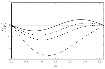
Figure 1: Reaction term $f(\varphi)$ for $k_{u}=1$ and different values of the applied field. The solid line shows the profile for the static solution $h_{a}=0$ for which $\varphi=0$ and $\varphi=\pi$ are equally stable. As the magnetic field increases $\varphi=0$ augments its stability while $\varphi=\pi$ gradually loses stability until it becomes unstable at sufficiently large applied field. In the figure the short dashed line, the dot-dashed line and the long dashed line correspond to dimensionless fields $h_{a}=0.5,1\text{ and }2.5$ respectively

The evolution of an initial condition $\varphi(x,0)$ under Eq. (17) has been fully studied for all types of reaction terms. It is known that in the bistable regime there is a unique traveling wave solution joining the two stable states, and in the monostable state, here $h_{a}>k_{u}$, there is a continuum of traveling wave solutions Fife and Mcleod (1977); Aronson and Weinberger (1978). In the bistable case a suitable initial condition evolves into the unique traveling wave Fife and Mcleod (1977); Aronson and Weinberger (1978) and in the monostable case it evolves into the traveling wave of minimal speed. The problem in this regime is to determine this minimal speed. The initial condition in the present case is a static HH or TT domain wall which satisfies the hypothesis of Fife and Mcleod (1977). For the sake of completeness we recall the main facts needed to determine the speed of the domain wall.

It is convenient to introduce a change of variables in order to apply directly the standard mathematical results. Going to the moving frame $\eta=\xi-(\beta U/\alpha)\tau$ and introducing the new independent variable $\phi=1-\varphi/\pi$, Eq.(17) becomes

$$\alpha\frac{\partial\phi}{\partial\tau}=D\phi_{\eta\eta}+F(\phi),\text{ with }F(\phi)=\frac{\sin\pi\phi}{\pi}(h_{a}-k_{u}\cos\pi\phi)$$ (20)

and $D=k_{u}/2$. In these new variables, the reaction term $F(\phi)$ satisfies $F(0)=F(1)=0$ and for $h_{a}<k_{u}$ is bistable, that is, $F<0$ in $(0,a)$, $F>0$ in $(a,1)$, $0<a<1$ . If $h_{a}\geq k_{u}$ it is monostable, i.e., $F>0$ in $(0,1)$.

This equation has the exact solution

$$\phi_{\sigma}(q)=\frac{2}{\pi}\arctan\left(\text{exp}(\sigma\sqrt{2}\,q)\right),\text{ with }\qquad c_{\sigma}=-\sigma\frac{h_{a}}{\sqrt{2}\,\alpha}.$$ (21)

where $q=\eta-c\tau,$ and $\sigma=\pm 1$. This exact solution is the unique solution in the bistable regime. In the monostable regime it is one of a continuum of solutions, it will be the solution to which a perturbation of the static state converges only if it is the front of minimal speed.

The standard theory Kolmogorov et al. (1937); Aronson and Weinberger (1978) guarantees that in the monostable regime suitable initial conditions will evolve into a traveling wave of minimal speed $\phi(\eta-c_{\text{min}}\tau)$ and the minimal speed $c_{\text{min}}$ satisfies

$$c_{\text{min}}\geq\frac{2}{\alpha}\sqrt{DF^{\prime}(0)}\equiv c_{\text{\tiny{KPP}}}.$$

We will show that the exact solution Eq. (21) is the solution selected by the dynamics for $0<h_{a}\leq 2k_{u}.$ For $h_{a}>2k_{u}$ the minimal speed is the KPP value. The minimal speed for a monotonic front of (20) satisfies the variational characterization Benguria and Depassier (1996)

$$c^{2}=\sup_{g}\frac{2D}{\alpha^{2}}\frac{\int_{0}^{1}F(u)g(u)du}{\int_{0}^{1}g^{2}(u)h^{-1}(u)du},$$ (22)

where $g(u)$ is an arbitrary positive function such that $h(u)=-g^{\prime}(u)>0$ and such that the integrals in (22) converge. In the case where an exact solution exists one can find the optimizing function $g(u)$, say $\hat{g}(u)$ for which the equal sign holds in (22). In effect, choosing as a trial function

$$g(u)=\left[\tan\left(\frac{\pi u}{2}\right)\right]^{-h_{a}/k_{u}}$$

we obtain

$$c^{2}\geq\frac{h_{a}^{2}}{2\alpha^{2}}\quad\text{for}\quad-2\leq h_{a}/k_{u}\leq 2.$$

This coincides with the exact solution so this is the optimizing trial function $\hat{g}$ and this is the minimal speed for $h_{a}\leq 2k_{u}.$ The exact solution (21) is the profile in this regime. For larger applied fields the speed, in the moving coordinate reference frame is $c_{\text{\tiny{KPP}}}$. The magnetization profile for $h_{a}>2k_{u}$ cannot be found analytically except at the transition point $h_{a}=2k_{u}$ but it shares the qualitative features of the exact solution.

In Fig. 2 we show the absolute value of the speed in the moving frame as a function of the applied field. We choose as parameters those of sample A3 of Thevenard et al. (2012), namely $M_{s}=36\text{ kA m}^{-1},K_{u}=40\text{ J m}^{-3},K_{d}=7415\text{ J m}^{-3},C_{ex}=2\times 10^{-13}\text{ J m}^{-1}$ and the Gilbert constant $\alpha=0.03$. The solid line shows the speed for all values of the applied field. The transition to the KPP regime occurs at $h_{a}=0.098$ in dimensionless units. For $0<h_{a}\leq 0.098$ the speed is that given by the exact solution Eq. (21) whereas for $h_{a}>0.098$ the speed is the $c_{\text{\tiny{KPP}}}$ value. The dot-dashed line shows the exact speed Eq. (21) which is not the speed of the domain wall in that parameter regime. Likewise the dashed line is the $c_{\text{\tiny{KPP}}}$ value, in the region where it is not the selected speed.

Figure 2: The solid line shows the domain wall speed as a function of the magnetic field for $\alpha=0.03,k_{u}=0.049$. For $h_{a}>2k_{u}$ the domain wall is of KPP type, for $h_{a}\leq 2k_{u}$ it is a pushed front.

In summary, going back to the original independent variable $\varphi$ and the laboratory frame, we find that the speed is given by

$$v_{\sigma}=\left\{\begin{array}[]{ll}\frac{\beta U}{\alpha}-\frac{\sigma h_{a}}{\sqrt{2}\,\alpha}&{\rm if}\,h_{a}\leq 2k_{u},\\ \frac{\beta U}{\alpha}-\frac{\sigma\sqrt{2k_{u}}}{\alpha}\sqrt{h_{a}-k_{u}}&{\rm if}\,h_{a}>2k_{u}.\end{array}\right.$$

In the first case the domain wall profile is determined by the analytic solution (21). In the original laboratory coordinates

$$\varphi_{\sigma}=\pi-\pi\phi_{\sigma}=\pi\phi_{-\sigma}=2\arctan\left(\text{exp}(-\sigma\sqrt{2}(\xi-v_{\sigma}\tau)\right),$$

so that

$$m_{1}=\sigma\tanh(\sqrt{2}(\xi-v_{\sigma}\tau)),\qquad\qquad m_{2}=\operatorname{sech}(\sqrt{2}(\xi-v_{\sigma}\tau)),$$

and

$$m_{3}=\sqrt{2}\sigma\operatorname{sech}(\sqrt{2}(\xi-v_{\sigma}\tau))\left(\frac{\sigma h_{a}}{\sqrt{2}\,\alpha}+U(1-\frac{\beta}{\alpha})+\sigma d\tanh(\sqrt{2}(\xi-v_{\sigma}\tau)\right).$$

The TT (HH) solution corresponds to $\sigma=1(-1)$ respectively.

The solution joining $-\pi$ to $0$ differs in chirality, the solution is analogous.

The speed and in plane components of the magnetization are unaffected by the DMI in this approximation, the out of plane component is distorted both by the applied field an current as well as the DMI. In Fig. 3 we have plotted the out of plane magnetization component for different values of the current and magnetic field. We use the same material parameters as in Fig. 2 and the values $D=1.6\times 10^{-3}$J m${}^{-2},\beta=10\alpha$.

Figure 3: The solid line shows the static out of plane magnetization. The dashed line shows the profile for vanishing current and applied field $H_{a}=0.088M_{s}.$ The dotted and dot-dashed lines show the profile for the same value of the magnetic field and for $u=\pm 400$ ms^-1 respectively.

V Summary

We studied the dynamics of an in-plane magnetized thin film including DMI under applied current and field acting along the easy axis when the perpendicular anisotropy is large. In this limit the out of plane magnetization is slaved to the in-plane components, the dynamics of which is governed by a reaction diffusion equation. Reaction diffusion dynamics is also encountered in the study of thin nanotubes however the role played by DMI in the dynamics is different for thin films. As mentioned in the introduction previous studies addressed the case of negligible $k_{d}$ and the limit of small DMI. Here we have considered the limit of large $k_{d}$ and find significant differences in the dynamics. For negligible $k_{d}$ Tretiakov and Abanov (2010) the domain wall width and speed depend on the DMI parameter and the magnetization spins. For small DMI Kravchuk (2014) and perpendicular anisotropy $k_{d}$ of order one the DMI does not affect the speed nor the in-plane magnetization profile in agreement with the present results. The effect of small DMI is the introduction of an asymmetric distortion in the out of plane component and a shift in the Walker field. In the case studied in this work the Walker field is not observed; instead, for sufficiently large applied field the domain wall slows down due to a change in the nature of the domain wall which goes from bistability to monostability and enters the so called KPP or pulled regime. Increasing the current does not lead to this change of behavior. Previous numerical work has reported the slowdown of the domain wall in thin films with very large axis anisotropy beyond a critical applied field due to spin wave emission Wieser et al. (2010); Wang et al. (2012); Wang and Wang (2014). Here we find the same qualitative feature, further study is required to obtain quantitative agreement with the numerical results and understand if the transition form pushed to pulled fronts is due to the emission of spin waves. The reaction diffusion equation filters out and gives no information on the emission of spin waves. In addition we were able to obtain a simple explicit expression for the out of plane magnetization showing the effect of the DMI and the motion on the profile showing an asymmetric distortion of the out of plane component when the domain wall moves. The perturbation method that we have used may prove useful to study other configurations where a Néel wall is preferred.

VI Acknowledgments

We acknowledge helpful discussions with E. Stockmeyer. This work was partially supported by Fondecyt (Chile) projects 114–1155 and 116–0856.

References

- Allwood et al. (2005) D. A. Allwood, G. Xiong, C. C. Faulkner, D. Atkinson, D. Petit, and R. P. Cowburn, Science 309, 1688 (2005).
- Stamps et al. (2014) R. L. Stamps, S. Breitkreutz, J. Akerman, A. V. Chumak, Y. Otani, G. E. W. Bauer, J.-U. Thiele, M. Bowen, S. A. Majetich, M. Klaeui, I. L. Prejbeanu, B. Dieny, N. M. Dempsey, and B. Hillebrands, J. Phys. D-Appl. Phys. 47, 333001 (2014).
- Landau and Lifshitz (1935) L. Landau and E. Lifshitz, Phys. Zs. Sowjet. 8, 153 (1935).
- Gilbert (1956) E. L. Gilbert, A Phenomenological Theory of Damping in Ferromagnetic Materials, dissertation, Illinois Institute of Technology (1956), reprinted in IEEE Trans. Mag. 40 (2014) 3443.
- Dzyaloshinsky (1958) I. Dzyaloshinsky, j. Phys. Chem. Solids 4, 241 (1958).
- Moriya (1960) T. Moriya, Phys. Rev. 120, 91 (1960).
- Thiaville et al. (2012) A. Thiaville, S. Rohart, E. Jué, V. Cros, and A. Fert, EPL 100, 57002 (2012).
- Emori et al. (2013) S. Emori, U. Bauer, S.-M. Ahn, E. Martinez, and G. S. D. Beach, Nat. Mater. 12, 611 (2013).
- Thevenard et al. (2017) L. Thevenard, B. Boutigny, N. Gusken, L. Becerra, C. Ulysse, S. Shihab, A. Lemaitre, J. V. Kim, V. Jeudy, and C. Gourdon, Phys. Rev. B 95, 054422 (2017).
- Tretiakov and Abanov (2010) O. A. Tretiakov and A. Abanov, Phys. Rev. Lett. 105, 157201 (2010).
- Kravchuk (2014) V. P. Kravchuk, J. Magn. Magn. Mater. 367, 9 (2014).
- Wang et al. (2015) W. Wang, M. Albert, M. Beg, M.-A. Bisotti, D. Chernyshenko, D. Cortes-Ortuno, I. Hawke, and H. Fangohr, Phys. Rev. Lett. 114, 087203 (2015).
- Zhuo and Sun (2016) F. Zhuo and Z. Z. Sun, Sci. Rep. 6, 25122 (2016).
- Wieser (2016) R. Wieser, Phys. Status Solidi B 253, 314 (2016).
- Wieser et al. (2010) R. Wieser, E. Y. Vedmedenko, and R. Wiesendanger, Phys. Rev. B 81, 024405 (2010).
- Wang et al. (2012) X. S. Wang, P. Yan, Y. H. Shen, G. E. W. Bauer, and X. R. Wang, Phys. Rev. Lett. 109, 167209 (2012).
- Hu and Wang (2013) B. Hu and X. R. Wang, Phys. Rev. Lett. 111, 027205 (2013).
- Wang and Wang (2014) X. S. Wang and X. R. Wang, Phys. Rev. B 90, 184415 (2014).
- Thevenard et al. (2012) L. Thevenard, S. A. Hussain, H. J. von Bardeleben, M. Bernard, A. Lemaitre, and C. Gourdon, Phys. Rev. B 85, 064419 (2012).
- Mikeska (1978) H. J. Mikeska, J. Phys. C: Solid State Phys. 11, L29 (1978).
- Garcia-Cervera and E (2001) C. Garcia-Cervera and W. E, J. Appl. Phys. 90, 370 (2001).
- Bazaliy (2007) Y. B. Bazaliy, Phys. Rev. B 76, 140402 (2007).
- Goussev et al. (2016) A. Goussev, J. M. Robbins, V. Slastikov, and O. A. Tretiakov, Phys. Rev. B 93, 054418 (2016).
- Lund et al. (2016) R. G. Lund, G. D. Chaves-O’Flynn, A. D. Kent, and C. B. Muratov, Phys. Rev. B 94, 144425 (2016).
- Thiaville et al. (2005) A. Thiaville, Y. Nakatani, J. Miltat, and Y. Suzuki, Europhys. Lett. 69, 990 (2005).
- Kolmogorov et al. (1937) A. Kolmogorov, I. Petrovskii, and N. Piscunov, Moscou Univ. Bull. Math. 1, 1 (1937).
- Hubert (1998) R. Hubert, A. Sch fer, Magnetic Domains (Springer-Verlag Berlin Heidelberg, 1998).
- Gioia and James (1997) G. Gioia and R. James, Proc. R. Soc. A-Math. Phys. Eng. Sci. 453, 213 (1997).
- Depassier (2015) M. C. Depassier, EPL 111, 27005 (2015).
- van Saarloos (1989) W. van Saarloos, Phys. Rev. A 39, 6367 (1989).
- Fife and Mcleod (1977) P. C. Fife and J. B. Mcleod, Arch. Ration. Mech. Anal. 65, 335 (1977).
- Aronson and Weinberger (1978) D. G. Aronson and H. F. Weinberger, Adv. Math. 30, 33 (1978).
- Benguria and Depassier (1996) R. D. Benguria and M. C. Depassier, Phys. Rev. Lett. 77, 1171 (1996).