Dynamic Network Identification From
Non-stationary Vector Autoregressive Time Series

Abstract

Learning the dynamics of complex systems features a large number of applications in data science. Graph-based modeling and inference underpins the most prominent family of approaches to learn complex dynamics due to their ability to capture the intrinsic sparsity of direct interactions in such systems. They also provide the user with interpretable graphs that unveil behavioral patterns and changes. To cope with the time-varying nature of interactions, this paper develops an estimation criterion and a solver to learn the parameters of a time-varying vector autoregressive model supported on a network of time series. The notion of local breakpoint is proposed to accommodate changes at individual edges. It contrasts with existing works, which assume that changes at all nodes are aligned in time. Numerical experiments validate the proposed schemes.

Index Terms—  Topology identification, vector autoregressive, group sparsity, breakpoint detection.

1 Introduction

Understanding the interactions among the parts of a complex dynamic system lies at the core of data science itself and countless applications in biology, sociology, neuroscience, finance, as well as engineering realms such as cybernetics, mechatronics, and control of industrial processes. Successfully learning the presence or evolution of these interactions allows forecasting and unveils complex behaviors typically by spotting causality relations [1]. To cope with the ever increasing complexity of the analyzed systems, traditional model-based paradigms are giving way to the more contemporary data-driven perspectives, where network-based approaches enjoy great popularity due to their ability to both discern between direct and indirect causality relations as well as to provide interaction graphs amenable to intuitive human interpretation. In this context, the time-varying nature of these interactions motivates inference schemes capable of handling non-stationarity multivariate data.

Inference from multiple time series has been traditionally addressed through vector autoregressive (VAR) models [2]. To cope with non-stationarity, VAR coefficients are assumed to evolve smoothly over time [3, 4, 5], to vary according to a hidden Markov model [6], or to remain constant over time intervals separated by structural breakpoints  [7, 8, 9, 10, 11, 12, 13]. Due to the high number of effective degrees of freedom of their models, these schemes can only satisfactorily estimate VAR coefficients if the data generating system experiences slow changes over time. To alleviate this difficulty, a natural approach is to exploit the fact that interactions among different parts of a complex system are generally mediated. For example, in an industrial plant where tank A is connected to B, B is connected to C, and C is not connected to A, the pressure of a fluid in a tank A affects directly the pressure of tank B and indirectly (through B) the pressure at tank C. Thus, a number of works focused on non-stationary data introduce graphs to capture this notion of direct interactions, either relying on graphical models [14, 15, 16, 17] or structural equation models [18, 19]. Unfortunately, these approaches can only deal with memoryless interactions, which limits their applicability to many real-world scenarios. Schemes that do account for memory and graph structure include models based on VAR [20] and models based on structural VAR models; see [21] and references therein. However, these methods can not handle non-stationarities. To sum up, none of the aforementioned schemes identifies interaction graphs in time-varying systems with memory. To the best of our knowledge, the only exception is [22], but it can only cope with slowly changing VAR coefficients.

To alleviate these limitations, the present paper relies on a time-varying VAR (TVAR) model to propose a novel estimation criterion for non-stationary data that accounts for memory and a network structure in the interactions. The resulting estimates provide allow forcasting and impulse response causality analysis [2, Ch. 2]. A major novelty is the notion of local structural breakpoint, which captures the intuitive fact that changes in the interactions need not be synchronized across the system; in contrast to most existing works. Furthermore, a low-complexity solver is proposed to minimize the aforementioned criterion and a windowing technique is proposed to accommodate prior information on the system dynamics and reduce computational complexity.

The rest of the paper is structured as follows. Sec. 2 introduces the model and the proposed criterion, with some practical considerations in Secs. 2.3 and 2.4; and Sec. 2.5 presents an iterative solver. Numerical experiments are described in Sec. 3 and conclusions in Sec. 4.

2 Dynamic network identification

After reviewing TVAR models and introducing the notion of time-varying causality graphs, this section proposes an estimation criterion and an iterative solver. Extensions and general considerations are provided subsequently.

2.1 Time-varying interaction graphs

A multivariate time series is a collection $\{\mathbf{y}_{t}\}_{t=1}^{T}$ of vectors $\mathbf{y}_{t}:=[y_{1,t},y_{2,t},\ldots,y_{P,t}]^{\top}$. The $i$-th (scalar) time series comprises the samples $\{y_{i,t}\}_{t=1}^{T}$ and can correspond e.g. with the activity over time of the $i$-th region of interest in a brain network, or with the measurements of the $i$-th sensor in a sensor network. A customary model for multivariate time series generated by non-stationary dynamic systems is the so-called $L$-th order TVAR model [2, Ch. 1]:

$$\mathbf{y}_{t}=\sum_{\ell=1}^{L}\mathbf{A}^{(\ell)}_{t}\mathbf{y}_{t-\ell}+\bm{\varepsilon}_{t}\vspace{-2mm}$$ (1)

where the matrix entries $\{a_{ij,t}^{(\ell)}\}_{i,j\in[1,P],t\in[1,T]}$ are the model coefficients and $\bm{\varepsilon}_{i,t}$ form the innovation process. Throughout, the notation $[m,n]$ with $m$ and $n$ integers satisfying $m\leq n$ will stand for $\{m,m+1,\ldots,n\}$. A time-invariant VAR model is a special case of (1) where $a_{ij,t}^{(\ell)}=a_{ij,t^{\prime}}^{(\ell)}~{}\forall(t,t^{\prime})$.

An insightful interpretation of time-varying VAR models stems from expressing (1) as

$$y_{i,t}=\textstyle\sum_{\ell=1}^{L}\textstyle\sum_{j=1}^{P}a_{ij,t}^{(\ell)}y_{j,t-\ell}+\bm{\varepsilon}_{i,t}$$ (2a)

$$=\sum_{j=1}^{P}\left[y_{j,t-1},y_{j,t-2},\ldots,y_{j,t-L}\right]\,\mathbf{a}_{ij,t}+\bm{\varepsilon}_{i,t}$$ (2b)

where $\mathbf{a}_{ij,t}:=[a_{ij,t}^{(1)},a_{ij,t}^{(2)},\ldots,a_{ij,t}^{(L)}]^{\top}$. From (2a), the $i$-th sequence $\{y_{i,t}\}_{t=1}^{T}$ equals the innovation plus the sum of all sequences $\{\{y_{p,t}\}_{t=1}^{T}\}_{p=1}^{P}$ after being filtered with a linear time-varying (LTV) filter with coefficients $\{a_{ij,t}^{(l)}\}_{l=1}^{L}$.

As described in Sec. 1, interactions among time series are generally indirect, which translates into many of these LTV filters being identically zero. To mathematically capture this interaction pattern, previous works consider the notion of graph associated with a time-invariant VAR process (see e.g. [20]), which is generalized next to time-varying VAR models (1). To this end, identify the $i$-th time series with the $i$-th vertex (or node) in the vertex set $\mathcal{V}:=[1,P]$ and define the time-varying edge set as $\mathcal{E}_{t}:=\{(i,j)\in\mathcal{V}\times\mathcal{V}:\mathbf{a}_{ij,t}\neq\mathbf{0}\}$. Thus, each edge of this time-varying graph can be thought of as an LTV filter, as depicted in Fig. 1.

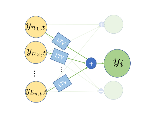
Fig. 1: Graph associated with a TVAR model.

2.2 Proposed estimation criterion

The main goal of this paper is to estimate $\{\{\mathbf{A}^{(\ell)}_{t}\}_{\ell=1}^{L}\}_{t=L+1}^{T}$ given $\{\mathbf{y}_{t}\}_{t=1}^{T}$. Without additional assumptions, reasonable estimates cannot be found because the number of unknowns is $(T-L)P^{2}L$ whereas the number of samples is just $PL$. This difficulty is typically alleviated by assuming certain structure usually found in real-world dynamic systems. As detailed next, the structure adopted here embodies both the sparsity of causal interactions and the spatial locality of changes in those interactions.

The proposed estimation criterion is given by

$$\min_{\{\mathbf{A}^{(\ell)}_{t}\}} \sum_{t=L+1}^{T}\left\lVert\mathbf{y}_{t}-\sum_{\ell=1}^{L}\mathbf{A}^{(\ell)}_{t}\mathbf{y}_{t-\ell}\right\rVert_{2}^{2}$$ (3)

$$+\sum_{(i,j)} \bigg{(}\lambda\sum_{t=L+1}^{T}\left\lVert\mathbf{a}_{ij,t}\right\rVert_{2}+\gamma\sum_{t=L+2}^{T}\left\lVert\mathbf{a}_{ij,t}-\mathbf{a}_{ij,t-1}\right\rVert_{2}\bigg{)}\vspace{-2mm}$$

where the first term promotes estimates that fit the data and the two regularizers in parentheses are explained next. The regularization parameters $\lambda>0$ and $\gamma>0$ can be selected through cross-validation to balance the relative weight of data and prior information.

The first regularizer is a group-lasso penalty that promotes edge sparsity or, equivalently, that a large number of LTV filters $\mathbf{a}_{ij,t}$ are $\bm{0}$. As delineated in Secs. 1 and 2.1, this corresponds to the intuitive notion that most interactions in a complex network are indirect and therefore nodes are connected only with a small fraction of other nodes. This regularizer generalizes the one in [20] to time-varying graphs.

The second regularizer is a total-variation regularizer that promotes estimates where the LTV filters remain constant over time except for a relatively small number of time instants $\mathcal{T}_{i,j}:=\{t:a_{ij,t}^{(\ell)}\neq a_{ij,t-1}^{(\ell)}$ for some $\ell\}$ denoted as local breakpoints. This regularizer, together with the notion of local breakpoints, constitutes one of the major novelties of this paper and contrasts with the notion of structural (or global) breakpoints, defined as $\mathcal{T}:=\{t:\mathbf{A}^{(\ell)}_{t}\neq\mathbf{A}^{(\ell)}_{t-1}$for some $\ell\}$ and adopted in the literature; see e.g. [11, 12, 7, 8, 10]. These works promote solutions with few global breakpoints, and therefore all the LTV filter estimates change simultaneously at the same time for all nodes. In contrast, this work advocates promoting solutions with few local breakpoints, since it is expected that changes in the underlying dynamic system take place locally. For instance, in a chemical process, closing a valve between tank A and B affects the future interactions between their pressures, but does not generally affect interactions between the pressure of tanks C and D.

2.3 Data windowing

In practice, the time series are expected to evolve at a faster time scale than the underlying system that generates them. In many applications, such as control of industrial processes, the opposite would imply that the sampling interval needs to be increased. If this is the case, it may be beneficial to assume that $\mathbf{A}^{(\ell)}_{t}$ remain constant within a certain window since this would decrease the number of coefficients to estimate and therefore would improve estimation performance.

To introduce this windowing technique let ${\color[rgb]{0,0,0}\mathcal{W}}_{{\color[rgb]{0,0,0}{n}}}\subset[L+1,T]$ denote the set of indices in the ${{\color[rgb]{0,0,0}{n}}}$-th window, ${{\color[rgb]{0,0,0}{n}}}=1,\ldots,{{\color[rgb]{0,0,0}{N}}}$, and let ${{\color[rgb]{0,0,0}{n}}}(t)={{\color[rgb]{0,0,0}{n}}}_{0}$ if $t\in{\color[rgb]{0,0,0}\mathcal{W}}_{{{\color[rgb]{0,0,0}{n}}}_{0}}$. If $\mathbf{A}^{(\ell)}_{t}=\tilde{\mathbf{A}}^{(\ell)}_{{{\color[rgb]{0,0,0}{n}}}(t)}~{}\forall t$, then (3) becomes

$$\min_{\{\tilde{\mathbf{A}}^{(\ell)}_{t}\}}\textstyle\sum_{t=L+1}^{T}\left\lVert\mathbf{y}_{t}-\textstyle\sum_{\ell=1}^{L}\tilde{\mathbf{A}}^{(\ell)}_{{{\color[rgb]{0,0,0}{n}}}(t)}\mathbf{y}_{t-\ell}\right\rVert_{2}^{2}+\sum_{(i,j)}$$ (4)

$$\bigg{(}\lambda\sum_{t=L+1}^{T}\left\lVert\tilde{\mathbf{a}}_{ij,{{\color[rgb]{0,0,0}{n}}}(t)}\right\rVert_{2}+\gamma\sum_{t=L+2}^{T}\left\lVert\tilde{\mathbf{a}}_{ij,{{\color[rgb]{0,0,0}{n}}}(t)}-\tilde{\mathbf{a}}_{ij,{{\color[rgb]{0,0,0}{n}}}(t-1)}\right\rVert_{2}\bigg{)}$$

where $\tilde{\mathbf{a}}_{ij,t}$ is correspondingly defined in terms of $\tilde{\mathbf{A}}^{(\ell)}_{t}$. Absorbing scaling factors in the regularization parameters, (4) boils down to

$$\min_{\{\tilde{\mathbf{A}}^{(\ell)}_{t}\}} \sum_{{{\color[rgb]{0,0,0}{n}}}=1}^{{\color[rgb]{0,0,0}{N}}}\sum_{t\in{\color[rgb]{0,0,0}\mathcal{W}}_{{\color[rgb]{0,0,0}{n}}}}\left\lVert\mathbf{y}_{t}-\sum_{\ell=1}^{L}\tilde{\mathbf{A}}^{(\ell)}_{{{\color[rgb]{0,0,0}{n}}}}\mathbf{y}_{t-\ell}\right\rVert_{2}^{2}$$ (5)

$$+\sum_{(i,j)} \bigg{(}\lambda\sum_{{{\color[rgb]{0,0,0}{n}}}=1}^{{\color[rgb]{0,0,0}{N}}}\left\lVert\tilde{\mathbf{a}}_{ij,{{\color[rgb]{0,0,0}{n}}}}\right\rVert_{2}+\gamma\sum_{{{\color[rgb]{0,0,0}{n}}}=2}^{{\color[rgb]{0,0,0}{N}}}\left\lVert\tilde{\mathbf{a}}_{ij,{{\color[rgb]{0,0,0}{n}}}}-\tilde{\mathbf{a}}_{ij,{{\color[rgb]{0,0,0}{n}}}-1}\right\rVert_{2}\bigg{)}.$$

Note that, while $LP^{2}(T-L)$ coefficients need to be estimated in (3), this number reduces to $LP^{2}N$ in (5).

Besides an improvement in the estimation performance (5) when the length of the windows is attuned to the dynamics of the system, it can be shown that the objective function becomes strongly convex if windows are sufficiently large, which speeds up the convergence of the algorithm in Sec. 2.5 (convergence becomes linear). The caveat here is a loss of temporal resolution: if one wishes to detect local breakpoints and two or more changes are produced in the same LTV filter within a single window, then the algorithm will only detect at most a single breakpoint. This effect can be counteracted by applying a screening techniques along the lines of [11].

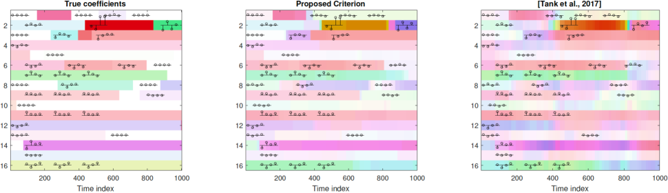
Fig. 2: Comparison between the estimates of the proposed criterion and the one in (Tank et al., 2017) [12]

2.4 Choice of parameters

Regularization parameters, in this case $\lambda$ and $\gamma$, are conventionally set through cross-validation. However, such a task may be challenging when dealing with non-stationary data. If one decides to carry out ${{\color[rgb]{0,0,0}{M}}}$-fold cross validation, forming ${{\color[rgb]{0,0,0}{M}}}$ sets of consecutive samples is not appealing since the estimate of the fitting error in the validation set will become artificially high and not informative about whether the algorithm is learning changes in the VAR coefficients.

To circumvent this limitation, the proposed technique forms the aforementioned sets by skipping one out of ${{\color[rgb]{0,0,0}{M}}}$ time samples. The estimator for the ${{\color[rgb]{0,0,0}{m}}}$-th fold becomes

$$\min_{\{\tilde{\mathbf{A}}^{(\ell)}_{t}\}} \sum_{{{\color[rgb]{0,0,0}{n}}}=1}^{{\color[rgb]{0,0,0}{N}}}\underset{t~{}\mathrm{mod}{{\color[rgb]{0,0,0}{M}}}\neq{{\color[rgb]{0,0,0}{m}}}}{\sum_{t\in{\color[rgb]{0,0,0}\mathcal{W}}_{{\color[rgb]{0,0,0}{n}}}}}\left\lVert\mathbf{y}_{t}-\sum_{\ell=1}^{L}\tilde{\mathbf{A}}^{(\ell)}_{{{\color[rgb]{0,0,0}{n}}}}\mathbf{y}_{t-\ell}\right\rVert_{2}^{2}$$ (6)

$$+\sum_{(i,j)} \bigg{(}\lambda\sum_{{{\color[rgb]{0,0,0}{n}}}=1}^{{\color[rgb]{0,0,0}{N}}}\left\lVert\tilde{\mathbf{a}}_{ij,{{\color[rgb]{0,0,0}{n}}}}\right\rVert_{2}+\gamma\sum_{{{\color[rgb]{0,0,0}{n}}}=2}^{{\color[rgb]{0,0,0}{N}}}\left\lVert\tilde{\mathbf{a}}_{ij,{{\color[rgb]{0,0,0}{n}}}}-\tilde{\mathbf{a}}_{ij,{{\color[rgb]{0,0,0}{n}}}-1}\right\rVert_{2}\bigg{)}.$$

Admittedly, all vectors $\{\mathbf{y}_{t}\}_{t}$ will still show up in all folds, but only as regressors in those folds where they are not target vectors. Indeed, this does not cause any problem from a theoretical standpoint and the performance observed in the numerical tests supports this approach.

2.5 Iterative solver

This section outlines the derivation of an ADMM-based algorithm proposed to solve (3). Define $\mathbf{Z}$ as the block-diagonal matrix with blocks $({\mathbf{x}^{\top}_{q+1}},$ ${\mathbf{x}^{\top}_{q+2}},\ldots,{\mathbf{x}^{\top}_{T}})$, with ${\mathbf{x}^{\top}_{t}}:=[\mathbf{y}_{t-1}^{\top}\ldots\mathbf{y}_{t-q}^{\top}]$; $\mathbf{B}:=[\mathbf{B}_{q+1}^{\top},\ldots,$ $\mathbf{B}_{T}^{\top}]$, with $\mathbf{B}_{t}:=\big{[}\mathbf{A}^{(1)}_{t},\mathbf{A}^{(2)}_{t},\ldots,\mathbf{A}^{(q)}_{t}\big{]}^{\top}$; and $\mathbf{Y}:=\left[\mathbf{y}_{q+1},\ldots,\mathbf{y}_{T}\right]^{\top}$. Then (3) can be rewritten as

$$\arg\min_{\mathbf{B}}\frac{1}{2}\left\lVert\mathbf{Y}-\mathbf{Z}\mathbf{B}\right\rVert_{F}^{2}+\lambda\Omega_{GL}(\mathbf{B})+\gamma\Omega_{GTV}(\mathbf{B})$$ (7)

where $\Omega_{GL}(\mathbf{B})=\sum_{(i,j)}\sum_{t=L+1}^{T}\left\lVert\mathbf{a}_{ij,t}\right\rVert_{2}$, and $\Omega_{GTV}(\mathbf{B})=\sum_{(i,j)}\sum_{t=L+1}^{T}\left\lVert\mathbf{a}_{ij,t+1}-\mathbf{a}_{ij,t}\right\rVert_{2}$. Upon defining

$$\mathbf{D}:=\begin{bmatrix}-\mathbf{I}&\mathbf{I}&\mathbf{0}&\ldots&\mathbf{0}\\ \mathbf{0}&-\mathbf{I}&\mathbf{I}&&\vdots\\ \vdots&\ddots&\ddots&\ddots&\\ \mathbf{0}&&\ldots&-\mathbf{I}&\mathbf{I}\end{bmatrix},\vspace{2mm}$$

$\Omega_{GTV}(\mathbf{B})$ can be expressed as $\Omega_{GL}(\mathbf{D}\mathbf{B})$. This allows to rewrite (7) along the lines of [23] for solving via ADMM

$$\arg\min_{\mathbf{B},\mathbf{\Theta},\mathbf{C}} \;\frac{1}{2}\left\lVert\mathbf{Y}-\mathbf{Z}\mathbf{B}\right\rVert^{2}_{F}+\lambda\Omega_{GL}(\mathbf{\Theta})+\gamma\Omega_{GL}(\mathbf{C}),$$

$$\mathrm{s.to} \;\mathbf{D}\mathbf{B}=\mathbf{\Theta},\;\mathbf{B}=\mathbf{C}$$ (8)

The ADMM for the $\rho$-augmented Lagrangian with scaled dual variables $\mathbf{U}$ and $\mathbf{V}$ computes for each iteration $k$:

$$\mathbf{B}^{[k+1]} :=\left(\mathbf{Z}^{\top}\mathbf{Z}/\rho+\mathbf{I}+\mathbf{D}^{\top}\mathbf{D}\right)^{\dagger}$$ (9)

$$\big{(}\mathbf{Z}^{\top}\mathbf{Y}/\rho+\mathbf{C}^{[k]}-\mathbf{V}^{[k]}+\mathbf{D}^{\top}(\mathbf{\Theta}^{[k]}-\mathbf{U}^{[k]})\big{)}$$

$$\bm{\theta}_{ij,t}^{[k+1]} :=\mathrm{prox}_{\lambda/\rho\left\lVert\cdot\right\rVert_{2}}({\mathbf{b}_{ij,t}^{[k+1]}-\mathbf{b}_{ij,t-1}^{[k+1]}-\mathbf{u}_{ij,t-1}^{[k+1]}})$$ (10)

$$\mathbf{c}_{ij,t}^{[k+1]} :=\mathrm{prox}_{\lambda/\rho\left\lVert\cdot\right\rVert_{2}}({\mathbf{b}_{ij,t}^{[k+1]}-\mathbf{v}_{ij,t}^{[k+1]}})$$ (11)

$$\mathbf{U}^{[k+1]} :=\mathbf{U}^{[k]}+(\mathbf{D}\mathbf{B}^{[k+1]}-\mathbf{\Theta}^{[k+1]})$$ (12)

$$\mathbf{V}^{[k+1]} :=\mathbf{V}^{[k]}+(\mathbf{B}^{[k+1]}-\mathbf{C}^{[k+1]})$$ (13)

and it is summarized in Proc. 1. The update (9) can be efficiently computed by exploiting the tri-diagonal strucutre of $\mathbf{Z}$ and $\mathbf{D}$. The updates in (10) and (11) exploit the fact that the resulting prox operators are separable per $(i,j)$ and can be expressed in terms of a group-soft-thresholding operator [24].

Procedure 1 ADMM solver for dynamic network ID

Input: $\lambda,\gamma$, data $\{\mathbf{y}_{t}\}_{t=1}^{T}$
Output: matrix $\mathbf{B}$ containing VAR coefficients

1:for $k=1,\ldots$ until convergence do

2:     Update $\mathbf{B}_{t}$ via (9)$\triangleright$ Block-Tridiagonal system

3:     for $t\in[L+1,T]$ do

4:         for $(i,j)\in[1,P]^{2}$ do $\triangleright$ Group-soft thresholding

5:              Update $\mathbf{c}_{ij,t},\mathbf{\theta}_{ij,t-1}$ via (10,11)               

6:     Update $\mathbf{U},\mathbf{V}$ via (12,13) $\triangleright$ Dual update

3 Numerical experiments

A simple experiment is shown next to validate the proposed estimator. An Erdos-Renyi [25] random graph $\mathcal{G}_{0}$ is generated with $P={\color[rgb]{0,0,0}4}$ nodes and an edge probability of $P_{0}^{(i,j)}:={\color[rgb]{0,0,0}0.5}$ if $i\neq j$ and $P_{0}^{(i,j)}:=0$ if $i=j$. An $(L={\color[rgb]{0,0,0}4})$-order TVAR model is generated, with initial VAR coefficients $\{\mathbf{A}^{(\ell)}_{L+1}\}_{\ell=1}^{L}$ over $\mathcal{G}_{0}$ drawn from a standard normal distribution and scaled to ensure stability [2, chapter 1]. Local breakpoints are generated at $N_{b}={\color[rgb]{0,0,0}100}$ uniformly spaced time instants $\mathcal{T}_{b}:=\{t_{b1},t_{b2},\ldots,t_{bN_{b}}\}$, and for each $t_{b}\in\mathcal{T}_{b}$ a pair of nodes $(i_{b},j_{b})$ is selected uniformly at random, generating a local breakpoint at the triplet $(t_{b},i_{b},j_{b})$. For each breakpoint $b$, the VAR coefficients $\mathbf{a}_{i_{b}j_{b},t_{b}}$ and the edge set $\mathcal{E}_{t}$ are changed as follows: if $(i_{b},j_{b})\in\mathcal{E}_{t_{b}-1}$, $\mathbf{a}_{i_{b}j_{b},t_{b}}$ is set to $\mathbf{0}$ with probability $P_{z}:={\color[rgb]{0,0,0}0.4}$; otherwise, a new standard Gaussian coefficient vector $\mathbf{a}_{i_{b}j_{b},t_{b}}$ is generated and scaled to keep stability. A realization of this TVAR process is generated by drawing $\{\mathbf{y}_{\ell}\}_{\ell=1}^{L}$ and $\{\bm{\varepsilon}_{t}\}_{t=L+1}^{T}$ i.i.d from a zero-mean Gaussian distribution with variance $\sigma_{\epsilon}^{2}:={\color[rgb]{0,0,0}0.03}$.

Fig. 2 compares the true coefficients with the estimates obtained by the proposed criterion and the one in [12]. The latter only detects global (but not local) breakpoints. The windowing described in Sec. 2.3 selects subperiods of length $N=21$, and $\lambda$ and $\gamma$ have been selected using the cross-validation scheme described in Sec. 2.4, both for the proposed algorithm and the one in [12] (which only uses $\lambda$).

In each subfigure, each horizontal band corresponds to a pair of nodes, and the horizontal axis represents time. The LTV impulse response vectors $\mathbf{a}_{ij,t}/\left\lVert\mathbf{a}_{ij,t}\right\rVert$ are mapped to colors in an HSV space, being assigned similar hue if their unitary counterparts $\mathbf{a}_{ij,t}/\left\lVert\mathbf{a}_{ij,t}\right\rVert$ are closeby. The value (brightness) is set proportional to $\left\lVert\mathbf{a}_{ij,t}\right\rVert$, so responses close to $\mathbf{0}$ appear close to white, whereas impulse responses with a larger $\ell_{2}$-norm will appear in a darker color. The stems appearing between some pairs of breakpoints represent filter coefficients of $\mathbf{a}_{ij,t}$ during the segment they lie on.

It is observed that the proposed algorithm could detect most of the local breakpoints and correctly identifies segments of stationarity. On the other hand, the competing algorithm yields a high number of false positives as expected.

4 Conclusions

Dynamic networks can be identified using the notion of local breakpoints, when VAR coefficient changes appear in a small number of edges. The proposed technique involves three novelties: a regularized criterion, a windowing technique, and a cross-validation scheme. Simulation experiments encourage further research along these lines.

References

- [1] C. W. J. Granger, “Some recent development in a concept of causality,” J. Econometrics, vol. 39, no. 1-2, pp. 199–211, Sep. 1988.
- [2] H. Lütkepohl, New Introduction to Multiple Time Series Analysis, Springer, 2005.
- [3] J. R. Sato, P. A. Morettin, P. R. Arantes, and E. Amaro Jr, “Wavelet based time-varying vector autoregressive modelling,” Comput. Statist. Data Anal., vol. 51, no. 12, pp. 5847–5866, 2007.
- [4] R. Dahlhaus, “Locally stationary processes,” in Handbook of statistics, vol. 30, pp. 351–413. Elsevier, 2012.
- [5] M. Niedźwiecki, M. Ciołek, and Y. Kajikawa, “On adaptive covariance and spectrum estimation of locally stationary multivariate processes,” Automatica, vol. 82, pp. 1–12, 2017.
- [6] E. Fox, E. B. Sudderth, M. I. Jordan, and A. S. Willsky, “Bayesian nonparametric inference of switching dynamic linear models,” IEEE Trans. Sig. Process., vol. 59, no. 4, pp. 1569–1585, Apr. 2011.
- [7] H. Ombao, R. Von Sachs, and W. Guo, “Slex analysis of multivariate nonstationary time series,” J. American Stat. Assoc., vol. 100, no. 470, pp. 519–531, 2005.
- [8] A. Aue, S. Hörmann, L. Horváth, M. Reimherr, et al., “Break detection in the covariance structure of multivariate time series models,” The Annals of Statistics, vol. 37, no. 6B, pp. 4046–4087, 2009.
- [9] H. Cho and P. Fryzlewicz, “Multiple-change-point detection for high dimensional time series via sparsified binary segmentation,” Journal of the Royal Statistical Society: Series B (Statistical Methodology), vol. 77, no. 2, pp. 475–507, 2015.
- [10] H. Cho et al., “Change-point detection in panel data via double cusum statistic,” Electronic Journal of Statistics, vol. 10, no. 2, pp. 2000–2038, 2016.
- [11] A. Safikhani and A. Shojaie, “Structural break detection in high-dimensional non-stationary var models,” arXiv preprint arXiv:1708.02736, 2017.
- [12] A. Tank, E. B Fox, and A. Shojaie, “An efficient admm algorithm for structural break detection in multivariate time series,” arXiv preprint arXiv:1711.08392, 2017.
- [13] H. Ohlsson, L. Ljung, and S. Boyd, “Segmentation of arx-models using sum-of-norms regularization,” Automatica, vol. 46, no. 6, pp. 1107–1111, 2010.
- [14] M. Kolar, Le Song, Amr A., and E. P. Xing, “Estimating time-varying networks,” The Annals of Applied Statistics, pp. 94–123, 2010.
- [15] J. Friedman, T. Hastie, and R. Tibshirani, “Sparse inverse covariance estimation with the graphical lasso,” Biostatistics, vol. 9, no. 3, pp. 432–441, 2008.
- [16] D. Angelosante and G. B. Giannakis, “Sparse graphical modeling of piecewise-stationary time series,” in Proc. IEEE Int. Conf. Acoust., Speech, Sig. Process., Prague, Czech Republic, 2011.
- [17] D. Hallac, Youngsuk Park, S. Boyd, and J. Leskovec, “Network inference via the time-varying graphical lasso,” in Proceedings of the 23rd ACM SIGKDD International Conference on Knowledge Discovery and Data Mining. ACM, 2017, pp. 205–213.
- [18] Y. Shen, B. Baingana, and G. B. Giannakis, “Tensor decompositions for identifying directed graph topologies and tracking dynamic networks,” IEEE Transactions on Signal Processing, vol. 65, no. 14, pp. 3675–3687, 2017.
- [19] B. Baingana and G. B. Giannakis, “Tracking switched dynamic network topologies from information cascades,” IEEE Trans. Sig. Process., vol. 65, no. 4, pp. 985–997, 2017.
- [20] A. Bolstad, B. D. Van Veen, and R. Nowak, “Causal network inference via group sparse regularization,” IEEE Trans. Sig. Process., vol. 59, no. 6, pp. 2628–2641, Jun. 2011.
- [21] Y. Shen, B. Baingana, and G. B. Giannakis, “Nonlinear structural vector autoregressive models for inferring effective brain network connectivity,” arXiv preprint arXiv:1610.06551, 2016.
- [22] B. Zaman, L. M. López-Ramos, D. Romero, and B. Beferull-Lozano, “Online topology estimation for vector autoregressive processes in data networks,” in Proc. IEEE Int. Workshop Comput. Advances Multi-Sensor Adaptive Process., Curaçao, NL, Dec 2017.
- [23] Bo Wahlberg, Stephen Boyd, Mariette Annergren, and Yang Wang, “An admm algorithm for a class of total variation regularized estimation problems,” IFAC Proceedings Volumes, vol. 45, no. 16, pp. 83–88, 2012.
- [24] S. Boyd, N. Parikh, E. Chu, B. Peleato, and J. Eckstein, “Distributed optimization and statistical learning via the altern. dir. method of multipliers,” Foundations Trends Mach. Learn., vol. 3, no. 1, pp. 1–122, Jan. 2011.
- [25] E. D. Kolaczyk, Statistical Analysis of Network Data: Methods and Models, Springer, New York, 2009.