Discrimination of discord in separable Gaussian states

Abstract

Consider two bosonic modes which are prepared in one of two possible Gaussian states with the same local energy: either a tensor-product thermal state (with zero correlations) or a separable Gaussian state with maximal correlations (with both classical and quantum correlations, the latter being quantified by quantum discord). For the discrimination of these states, we compare the optimal joint coherent measurement with the best local measurement based on single-mode Gaussian detections. We show how the coherent measurement always strictly outperforms the local detection strategy for both single- and multi-copy discrimination. This means that using local Gaussian measurements (assisted by classical communication) is strictly suboptimal in detecting discord. A better performance may only be achieved by either using non Gaussian measurements (non linear optics) or coherent non-local measurements.

1 Introduction

Quantum correlations are today recognized as a fundamental physical resource in quantum information [3, 1, 2, 4, 5]. For pure states of a quantum system, quantum correlations are exactly the same as entanglement. However, this equivalence fails when general mixed states are taken into account: Separable mixed states can still have correlations which cannot be simulated by any classical probability distribution [6, 7, 8]. These correlations are quantified by the concept of quantum discord, whose definition is related to inequivalent extensions of the mutual information from the classical to the quantum setting.

On the one hand, the mutual information $I(X:Y)$ between two classical variables, $X$ and $Y$, can be extended to the quantum mutual information between two quantum systems, $A$ and $B$, defined by

$$I_{tot}(A:B)=S(A)+S(B)-S(A,B)~{},$$ (1)

where $S(.)$ is the von Neumann entropy. This quantity accounts for all the correlations between the two quantum systems. On the other hand, another possible extension of $I(X:Y)$ is given by the entropic quantity

$$C(A:B):=S(A)-\inf_{\mathcal{B}}S_{\mathcal{B}}(A|B)~{},$$ (2)

where $S_{\mathcal{B}}(A|B)$ is the conditional entropy of system $A$ given system $B$ being subject to a quantum measurement $\mathcal{B}$, i.e., a positive operator valued measure (POVM).

The quantity $C(A:B)$ is generally less than or equal to $I_{tot}(A:B)$, and can be interpreted as the maximal amount of classical correlations between $A$ and $B$. Quantum discord is therefore defined as the difference between total and classical correlations, i.e.,

$$D(A :B):=I_{tot}(A:B)-C(A:B)=S(B)-S(A,B)+\inf_{\mathcal{B}}S_{\mathcal{B}}(A|B)~{}.$$ (3)

In general, $C$ and $D$ are asymmetric quantities under system permutation $A\leftrightarrow B$, unless we consider symmetric quantum states, i.e., such that $\rho_{AB}=\rho_{BA}$.

In the continuous variable framework, systems $A$ and $B$ are typically bosonic modes in a Gaussian state. In this case, we may restrict the minimization in Eq. (3) from arbitrary measurements $\mathcal{B}$ to Gaussian measurements $\mathcal{G}$ and define the Gaussian discord [9, 10]. Gaussian discord can be easily computed and it has been proven to be the actual (unrestricted) quantum discord for a large family of Gaussian states [11]. In particular, this equivalence is true for the Gaussian states considered here.

In this paper, we study the performance of global and local detectors in discriminating the presence of correlations in bipartite Gaussian states. More precisely, we compare an optimal coherent detector with local Gaussian detectors in the discrimination of quantum discord and classical correlations, assuming either a tensor-product of single-mode thermal states or a correlated (but separable) two-mode thermal state. We quantify the advantage of the coherent detector both in the setting of single-copy discrimination and that of multi-copy discrimination (by comparing the error-exponents in the decaying error probability). Because this advantage is strictly larger than zero, one may hide classical information in the separable correlations of Gaussian states, therefore realizing a simple Gaussian form of quantum data hiding [12].

2 Discrimination scenario

Let us consider two bosonic modes, $A$ and $B$, prepared in a symmetric Gaussian state $\rho$. This state is randomly chosen from a binary ensemble $\{\rho_{0},\rho_{1}\}$ with uniform probability $p_{0}=p_{1}=1/2$. In other words, a bit of information $k=0,1$ is encoded into the state of the two bosonic modes. The two Gaussian states $\rho_{0}$ and $\rho_{1}$ are taken to be separable but with maximal difference in terms of correlations. We consider $\rho_{0}$ to be tensor product of two thermal states, so that it has zero discord ($D_{0}=0$) and zero classical correlations ($C_{0}=0$). For $\rho_{1}$, we consider a separable Gaussian state with the same energy as $\rho_{0}$ but maximally correlated, i.e., with maximal discord $D_{1}$ and maximal classical correlations $C_{1}$. In other words, for fixed energy, we are comparing a completely uncorrelated Gaussian state with the most correlated (but separable) Gaussian state, so that the bit of information is practically encoded in the absence or presence of correlations with maximal variations $\delta D:=D_{1}-D_{0}$ and $\delta C:=C_{1}-C_{0}$.

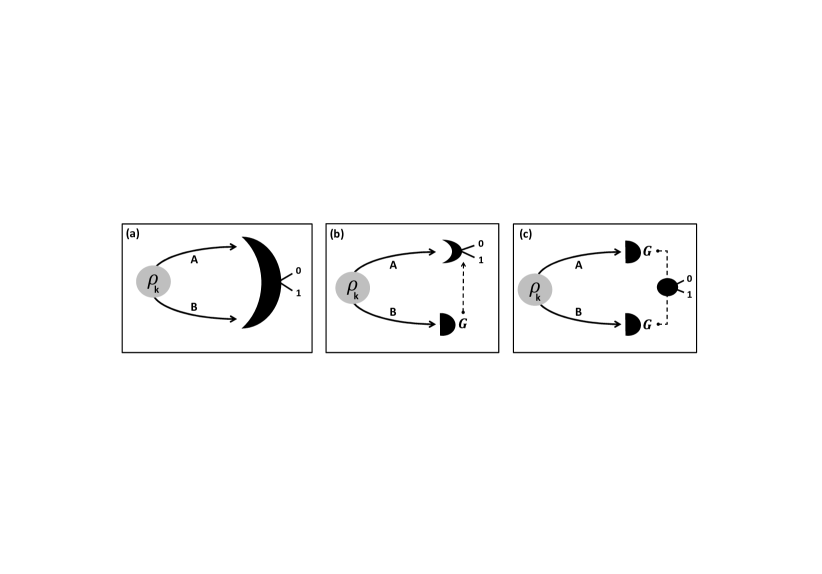
For state-discrimination, i.e., bit-decoding, we then consider two different types of detection as depicted in Fig. 1. First, we consider the optimal global measurement on both modes $A$ and $B$. This is given by the Helstrom POVM$\ \{E_{0},I-E_{0}\}$, with $E_{0}$ projecting on the positive part of $\rho_{0}-\rho_{1}$, which is clearly a non-Gaussian measurement. The minimum error probability is given by the Helstrom bound [13]

$$P=\frac{1}{2}[1-T(\rho_{0},\rho_{1})]~{},$$ (4)

where $T$ is the trace distance between the two states. Correspondingly, the information retrieved is equal to

$$I=1-H(P)~{},$$ (5)

where $H$ is the binary Shannon entropy.

Figure 1: Discrimination of two Gaussian states, $\rho_{0}$ and $\rho_{1}$, using a coherent detector (inset a), or using an incoherent detector based on a local Gaussian measurement followed by an Helstrom measurement (inset b), or using an incoherent detector based on two local Gaussian measurements whose outputs are suitably post-processed (inset c).

The second type of detection corresponds to local measurements (see Fig. 1). Here the decoder applies an optimal Gaussian measurement on mode $B$, followed by an optimal Helstrom POVM on mode $A$. This local measurement clearly represents an upper bound for all the possible local Gaussian measurements (where both the modes are detected by optimized Gaussian POVMs). This second scheme will be affected by an error probability which is generally bigger than before, i.e., $P_{loc}\geq P$, with retrieved information

$$I_{loc}=1-H(P_{loc})\leq I~{}.$$ (6)

Here we are interested in studying the behaviour of these quantities (probabilities and mutual informations) in terms of the encoded correlations, i.e., the variation of Gaussian discord $\delta D$ and the variation of classical correlations $\delta C$. In particular, we are interested in investigating the behaviour of the information gain $\Delta I:=I-I_{loc}\geq 0$ of the global detection versus the local one. We show that there is a strict separation $\Delta I>0$ so that global detection is proven to provide the best strategy in detecting such kinds of correlations.

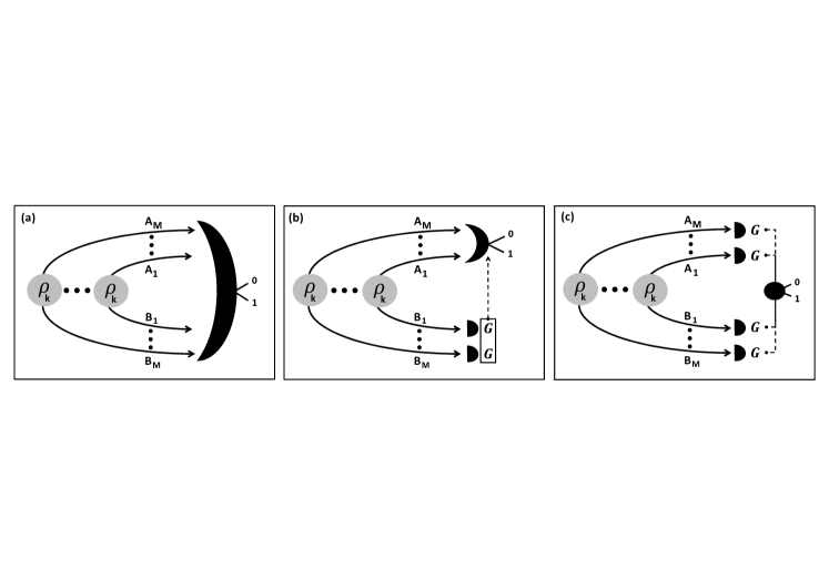
Figure 2: Multi-copy discrimination of two Gaussian states, $\rho_{0}$ and $\rho_{1}$, using an optimal coherent detector acting on all the modes. This is realized by an Helstrom POVM (inset a). Multi-copy discrimination of two Gaussian states, $\rho_{0}$ and $\rho_{1}$, using an incoherent detector based on a single-mode Gaussian measurements on modes $B$ followed by an Helstrom measurement on modes $A$ (inset b), or using an incoherent detector based single-mode Gaussian measurements on all the modes, whose outputs are suitably post-processed (inset c).

In general, the problem can be extended to multicopy discrimination, where the encoder prepares $M$ copies $\rho_{0}^{\otimes M}:=\rho_{0}\otimes\cdots\otimes\rho_{0}$ or $\rho_{1}^{\otimes M}:=\rho_{1}\otimes\cdots\otimes\rho_{1}$, with the same probability. In this generalization, we consider a decoder that either performs an optimal global measurement (Helstrom POVM) on all the collection of modes $A_{1},\ldots,A_{M},B_{1},\ldots,B_{M}$ (see Fig. 2) or a local measurement, composed of optimal local measurements on the $A$ modes, followed by an optimal Helstrom measurement on all the $B$ modes. This second strategy is clearly local in terms of the $A$-$B$ bipartition and it represents an upper bound for all the measurements based on single-mode Gaussian POVMs (see Fig. 2).

Suppose that the decoder applies an optimal global measurement. Then, for large number of copies ($M\gg 1$), the minimum error probability can be written as

$$P\approx\frac{1}{2}\exp(-\kappa M)~{},$$ (7)

where the error-probability exponent $\kappa=-\ln Q$ is provided by the quantum Chernoff bound (QCB) [14, 15]

$$Q=\inf_{0\leq s\leq 1}\mathrm{Tr}\left(\rho_{0}^{s}\rho_{1}^{1-s}\right)~{}.$$ (8)

By contrast, if the decoder performs the local measurement (Gaussian followed by Helstrom POVM), then the minimum error probability will have an error-probability exponent $\kappa_{loc}\leq\kappa$. As measures of the asymptotic gain we can consider the difference between the two error-exponents

$$\Delta:=\kappa-\kappa_{loc}\geq 0~{}.$$

As before, we are interested in studying the gain $\Delta$ in terms of the encoded correlations $\delta D$ and $\delta C$. In this case, we are able to prove that the gain is strictly positive and increasing in the correlations. In particular, we have $\Delta\rightarrow\Delta_{\max}>2$ for maximal correlations, i.e., for $\delta D\rightarrow 1$ and $\delta C\rightarrow+\infty$. Thus, the use of a global coherent measurement outperforms any local measurements based on single-mode Gaussian detectors for discriminating the presence or not of correlations in Gaussian states (both classical and quantum correlations).

3 Single-copy discrimination of two-mode Gaussian states

In our analysis we can reduce Gaussian states to zero-mean Gaussian states, which are fully characterized by their covariance matrix (CM). This is because displacements are local operations and therefore not related with their correlation properties. Since discord and classical correlations are defined as entropic quantities, they are invariant under local unitaries [8]. Thus, by using local Gaussian unitaries (corresponding to symplectic transformations in the phase-space), we can always reduce the CM of a symmetric Gaussian state $\rho$ of modes $A$ and $B$ into the normal form

$$\mathbf{V}(\mu,g,g^{\prime})=\left(\begin{array}[c]{cccc}\mu&&g&\\ &\mu&&g^{\prime}\\ g&&\mu&\\ &g^{\prime}&&\mu\end{array}\right)~{},$$ (9)

where the real parameters $\mu$, $g$ and $g^{\prime}$ must satisfy a set of bona-fide conditions [16]. These conditions are here equal to $\mu\geq 1$ and

$$\left|g\right|<\mu,~{}\left|g^{\prime}\right|<\mu,~{}\mu^{2}+gg^{\prime}-1\geq\mu\left|g+g^{\prime}\right|~{}.$$ (10)

The parameter $\mu$ quantifies the variance of the thermal noise which is present in each bosonic mode. In fact, the two reduced states $\rho^{A}=\mathrm{Tr}_{B}(\rho)$ and $\rho^{B}=\mathrm{Tr}_{A}(\rho)$ are identical thermal states with mean number of photons equal to $\bar{n}=(\mu-1)/2$. The two parameters $g$ and $g^{\prime}$ describe the correlations between the two modes. For $g=g^{\prime}=0$ we have zero correlations ($C_{0}=D_{0}=0$) and this is chosen to be the CM $\mathbf{V}_{0}$ of the first Gaussian state $\rho_{0}$. The other Gaussian state $\rho_{1}$ is chosen to be separable but with maximal correlations, both quantum and classical. Keeping fixed $\mu$, i.e., the energy of the state, the most correlated but still separable Gaussian state corresponds to the choice $g=g^{\prime}=\mu-1$, or equivalently $1-\mu$. This Gaussian state $\rho_{1}$ with CM $\mathbf{V}_{1}(\mu)=\mathbf{V}(\mu,\mu-1,\mu-1)$ has maximal classical correlations

$$C_{1}=h(\mu)-h\left(\frac{3\mu-1}{\mu+1}\right):=\delta C(\mu)~{},$$ (11)

and maximal quantum discord [11]

$$D_{1}=h(\mu)-h(2\mu-1)+h\left(\frac{3\mu-1}{\mu+1}\right):=\delta D(\mu)~{},$$ (12)

where $h(x)$ is von Neumann entropy given by the formula

$$h(x):=\left(\frac{x+1}{2}\right)\log_{2}\left(\frac{x+1}{2}\right)-\left(\frac{x-1}{2}\right)\log_{2}\left(\frac{x-1}{2}\right).$$ (13)

Our first aim is to derive the minimum error probability $P=P(\mu)$ in the discrimination of these two Gaussian states, by performing an optimal global measurement.

3.1 Performance of a global two-mode measurement

Given two Gaussian states, it is generally difficult to compute the exact performance of the optimal coherent detector, because of the trace distance involved in the Helstrom bound. Here we resort to easier-to-compute bounds in order to provide an estimate of the mimimum error probability. The first bound is the QCB (single-copy formula)

$$P\leq P^{+}=\frac{1}{2}\inf_{0\leq s\leq 1}Q_{s}~{},$$ (14)

where the s-overlap $Q_{s}$ is given by

$$Q_{s}=\mathrm{Tr}(\rho_{0}^{s}\rho_{1}^{1-s})~{}.$$ (15)

We have a closed formula [15, 17] for the s-overlap $Q_{s}$ in the case of multi-mode Gaussian states. Let us write this formula explicitly for the case of zero-mean two-mode Gaussian states. First introduce the two real functions

$$G_{s}(x):=\frac{2^{s}}{\left(x+1\right)^{s}-\left(x-1\right)^{s}},~{}~{}\Lambda_{s}(x):=\frac{\left(x+1\right)^{s}+\left(x-1\right)^{s}}{\left(x+1\right)^{s}-\left(x-1\right)^{s}}~{}.$$ (16)

Then, consider the symplectic decomposition of their CMs, $\mathbf{V}_{0}$ and $\mathbf{V}_{1}$, according to Williamson’s theorem [18]

$$\mathbf{V}_{0}=\mathbf{S}_{0}\left(\begin{array}[c]{cc}\alpha_{-}\mathbf{I}&\\ &\alpha_{+}\mathbf{I}\end{array}\right)\mathbf{S}_{0}^{T},~{}~{}~{}\mathbf{V}_{1}=\mathbf{S}_{1}\left(\begin{array}[c]{cc}\beta_{-}\mathbf{I}&\\ &\beta_{+}\mathbf{I}\end{array}\right)\mathbf{S}_{1}^{T}~{}.$$ (17)

Here $\alpha_{\pm}$ is the symplectic spectrum of $\mathbf{V}_{0}$ diagonalized by the symplectic matrix $\mathbf{S}_{0}$, and $\beta_{\pm}$ is the symplectic spectrum of $\mathbf{V}_{1}$ diagonalized by the symplectic $\mathbf{S}_{1}$ [4]. In this case, the $s$-overlap $Q_{s}$ of the QCB is given by the formula

$$Q_{s}=\Pi_{s}\left(\det\boldsymbol{\Sigma}_{s}\right)^{-1/2}$$ (18)

where

$$\Pi_{s}:=4G_{s}(\alpha_{+})G_{s}(\alpha_{-})G_{1-s}(\beta_{+})G_{1-s}(\beta_{-})$$ (19)

and

$$\boldsymbol{\Sigma}_{s}:=\mathbf{S}_{0}\left(\begin{array}[c]{cc}\Lambda_{s}(\alpha_{-})\mathbf{I}&\\ &\Lambda_{s}(\alpha_{+})\mathbf{I}\end{array}\right)\mathbf{S}_{0}^{T}+\mathbf{S}_{1}\left(\begin{array}[c]{cc}\Lambda_{1-s}(\beta_{-})\mathbf{I}&\\ &\Lambda_{1-s}(\beta_{+})\mathbf{I}\end{array}\right)\mathbf{S}_{1}^{T}.$$ (20)

In order to apply the formula to the Gaussian states of our discrimination problem, we have to derive the explicit symplectic decompositions of their CMs. In the case of the uncorrelated thermal state $\rho_{0}$, it is trivial to say that $\mathbf{V}_{0}$ is already in its diagonal Williamson’s form ($\mathbf{S}_{0}=\mathbf{I}$) with degenerate spectrum $\alpha_{+}=\alpha_{-}=\mu$. For the other CM $\mathbf{V}_{1}$, it is easy to check that this is diagonalized by a symplectic matrix of the form $\mathbf{S}_{1}=\mathbf{O}(\mathbf{L\oplus L)}$, where $\mathbf{O}$ is a special orthogonal matrix (therefore symplectic) and $\mathbf{L}$ is the squeezing matrix

$$\mathbf{L=}\left(\begin{array}[c]{cc}\frac{1}{\sqrt{\beta}}&\\ &\sqrt{\beta}\end{array}\right),~{}\beta:=\sqrt{2\mu-1}~{}.$$ (21)

The corresponding symplectic spectrum is degenerate and equal to $\beta_{+}=\beta_{-}=\beta$ (see Appendix A).

The numerator in the $s$-overlap is therefore equal to

$$\Pi_{s}:=4\left[G_{s}(\mu)G_{1-s}\left(\beta\right)\right]^{2}~{}.$$ (22)

At the denominator, we have the sigma-matrix

$$\boldsymbol{\Sigma}_{s}=\Lambda_{s}(\mu)(\mathbf{I\oplus I})+\Lambda_{1-s}\left(\beta\right)\mathbf{O}(\mathbf{L}^{2}\mathbf{\oplus L}^{2}\mathbf{)O}^{T}~{}.$$ (23)

Since the determinant does not change under orthogonal transformations, i.e., $\det\boldsymbol{\Sigma}_{s}=\det(\mathbf{O}^{T}\boldsymbol{\Sigma}_{s}\mathbf{O})$, we can replace $\boldsymbol{\Sigma}_{s}$ by the diagonal matrix

$$\boldsymbol{\Sigma}_{s} =\Lambda_{s}(\mu)(\mathbf{I\oplus I})+\Lambda_{1-s}\left(\beta\right)(\mathbf{L}^{2}\mathbf{\oplus L}^{2}\mathbf{)}$$

$$={\displaystyle\bigoplus\limits_{i=A,B}}\left(\begin{array}[c]{cc}\Lambda_{s}(\mu)+\frac{\Lambda_{1-s}\left(\beta\right)}{\beta}&\\ &\Lambda_{s}(\mu)+\beta\Lambda_{1-s}\left(\beta\right)\end{array}\right).$$ (26)

By replacing Eqs. (22) and (26) into Eq. (18), we get the analytical expression of the $s$-overlap $Q_{s}$ (not reported here for brevity). By optimizing in the $s$ parameter as in Eq. (14), we derive the QCB as a function of $\mu$, i.e., $P^{+}=P^{+}(\mu)$. In turn, this bound can be expressed in terms of the encoded Gaussian dicord $P^{+}=P^{+}(\delta D)$ and the encoded classical correlations $P^{+}=P^{+}(\delta C)$ by using Eqs. (11) and (12).

Now let us derive a lower bound to the error probability. A simple bound can be constructed using the quantum Battacharryya bound [15, 19]. In fact, we can write

$$P(\mu)\geq P^{-}(\mu):=\frac{1-\sqrt{1-B^{2}}}{2}~{},$$ (27)

where

$$B:=Q_{1/2}=\mathrm{Tr}(\sqrt{\rho_{0}}\sqrt{\rho_{1}})~{}.$$ (28)

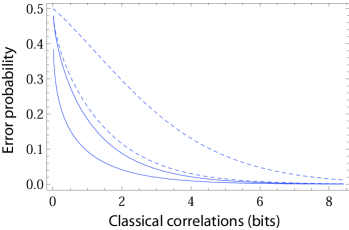
As before, we can express $P^{-}$ is terms of the encoded discord $\delta D$ and classical correlations $\delta C$. The behaviour of the two bounds $P^{+}$ and $P^{-}$ in terms of the correlations are shown in Fig. 3. As expected the error probability goes to zero in the limit of maximal discord $\delta D\rightarrow 1$ and maximal classical correlations $\delta C\rightarrow+\infty$.

Figure 3: Left panel. Upper ($P^{+}$) and lower ($P^{-}$) bounds to the error probability versus encoded discord $\delta D$ for the optimal global detector (solid lines) and the local detector (dashed lines). Right panel. The previous bounds are plotted versus the encoded classical correlations $\delta C$.

Clearly, from the previous bounds on the error probability we can derive upper and lower bounds for the mutual information

$$I_{-}(\mu)\leq I(\mu)\leq I_{+}(\mu)~{},$$ (29)

where

$$I_{+}(\mu):=1-H[P^{-}(\mu)]~{},$$ (30)

and

$$I_{-}(\mu):=1-H[P^{+}(\mu)]~{}.$$ (31)

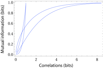
The two bounds, $I_{-}$ and $I_{+}$, can be expressed in terms of $\delta C$ and $\delta D$ and are plotted in Fig. 4.

Figure 4: Upper ($I_{+}$) and lower ($I_{-}$) bounds to the mutual information versus encoded discord (left curves) and encoded classical correlations (right curves)

3.2 Performance of local measurements

Here we estimate the minimum error probability which is achievable by using local detections. As discussed in the introduction, we consider a local Gaussian measurement followed by a local Helstrom measurement, which is an upper bound to considering two local Gaussian detections. The most general single-mode Gaussian POVM $\mathcal{G}$ has measurement operator $G(\mathbf{x}):=\pi^{-1}W(\mathbf{x})\sigma W(-\mathbf{x})$, where $\mathbf{x}\in\mathbb{R}^{2}$, $W(\mathbf{x})$ is the Weyl-displacement operator [4] and $\sigma$ is a zero-mean Gaussian state with CM

$$\mathbf{V}_{\sigma}=\eta\mathbf{R}(\theta)\left(\begin{array}[c]{cc}\lambda&\\ &\lambda^{-1}\end{array}\right)\mathbf{R}(-\theta)~{},$$ (32)

where $\eta\geq 1$, $\lambda>0$ and $\mathbf{R}(\theta)$ is the rotation matrix with angle $\theta$.

Since the encoding states are symmetric, there is no difference in where the first measurement is performed. Without loss of generality, we assume that mode $B$ is measured first. The reduced state of mode $B$ is a thermal state, no matter what the encoding is ($\rho_{0}^{B}=\rho_{1}^{B}$). This means that the outcome of the Gaussian measurement on mode $B$ does not contain any information on the encoded two-mode state. The effect of this measurement is only that of preparing conditional states on the other mode $A$. More precisely, if the encoded two-mode state were $\rho_{0}$, then the conditional state trivially coincides with the thermal reduced state $\rho_{0}^{A|B}=\rho_{0}^{A}$. By contrast, if the encoded state were $\rho_{1}$, then we have the remote preparation of a Gaussian state $\rho_{1}^{A|B}(\mathbf{a})$ with conditional CM [20]

$$\mathbf{V}_{A|B}=\mu\mathbf{I}-\mathbf{\tilde{V},~{}\tilde{V}}:=(\mu-1)^{2}(\mu\mathbf{I+V}_{\sigma})^{-1}~{},$$ (33)

and random displacement $\mathbf{a}$ depending on the outcome of the measurement $\mathbf{x}$. Since the classical outcome $\mathbf{x}$ is Gaussianly distributed, also the displacement $\mathbf{a}$ is Gaussianly-modulated, with a Gaussian $G_{\mathbf{\tilde{V}}}(\mathbf{a})$ having zero mean and classical CM $\mathbf{\tilde{V}}$.

Once the outcome $\mathbf{x}$ has been retrieved and therefore the remote displacement $\mathbf{a}$ is known, the aim of the second measurement is to distinguish between $\rho_{0}^{A|B}$ and $\rho_{1}^{A|B}(\mathbf{a})$. There will be a corresponding Helstrom POVM which projects on the positive part of $\gamma(\mathbf{a}):=\rho_{1}^{A|B}(\mathbf{a})-\rho_{0}^{A|B}$ with associated error probability

$$P_{loc}(\mathbf{a},\mathcal{G})=\frac{1}{2}\left[1-T\left(\rho_{1}^{A|B}(\mathbf{a}),\rho_{0}^{A|B}\right)\right]~{}.$$ (34)

By averaging over the random displacement, we derive the mean error probability

$$P_{loc}(\mathcal{G})=\int d\mathbf{a~{}}G_{\mathbf{\tilde{V}}}(\mathbf{a})P_{loc}(\mathbf{a},\mathcal{G})~{}.$$ (35)

Now the optimal performance is given by optimizing over all the Gaussian POVMs

$$P_{loc}=\min_{\mathcal{G}}P_{loc}(\mathcal{G})~{}.$$ (36)

In this case too we resort to upper and lower bounds. First we construct the upper bound using the QCB. We have

$$P_{loc}(\mathbf{a},\mathcal{G})\leq P_{loc}^{+}(\mathbf{a},\mathcal{G})=\frac{1}{2}\inf_{0\leq s\leq 1}Q_{s}(\mathbf{a},\mathcal{G})$$

where $Q_{s}$ must be computed here on the two Gaussian states $\rho_{0}^{A|B}$ (with zero mean and CM $\mu\mathbf{I}$) and $\rho_{1}^{A|B}(\mathbf{a})$, with random displacement $\mathbf{a}$ and CM $\mathbf{V}_{A|B}$. The latter has symplectic decomposition $\mathbf{V}_{A|B}=\nu_{A|B}\mathbf{S}_{A|B}\mathbf{S}_{A|B}^{T}$, with $\nu_{A|B}=\sqrt{\det\mathbf{V}_{A|B}}$ and $\mathbf{S}_{A|B}$ being a suitable symplectic matrix. In this case the s-overlap takes the form

$$Q_{s}(\mathbf{a},\mathcal{G})=\Pi_{s}\left(\det\boldsymbol{\Sigma}_{s}\right)^{-1/2}\exp\left(-\frac{\mathbf{a}^{T}\boldsymbol{\Sigma}_{s}^{-1}\mathbf{a}}{2}\right)~{},$$ (37)

where

$$\Pi_{s} =2G_{s}(\mu)G_{1-s}\left(\nu_{A|B}\right)~{},$$ (38)

$$\boldsymbol{\Sigma}_{s} =\Lambda_{s}(\mu)\mathbf{I}+\Lambda_{1-s}\left(\nu_{A|B}\right)\mathbf{S}_{A|B}\mathbf{S}_{A|B}^{T}~{}.$$ (39)

By averaging over the random displacement we get

$$P_{loc}^{+}(\mathcal{G})=\int d\mathbf{a~{}}G_{\mathbf{\tilde{V}}}(\mathbf{a})P_{loc}^{+}(\mathbf{a},\mathcal{G})=\frac{1}{2}\inf_{0\leq s\leq 1}Q_{s}(\mathcal{G})~{},$$ (40)

where

$$Q_{s}(\mathcal{G})=\frac{\Pi_{s}}{\sqrt{\det(\boldsymbol{\Sigma}_{s}+\mathbf{\tilde{V}})}}~{}.$$ (41)

As we show in the Appendix B, for any $0\leq s\leq 1$ we have that $Q_{s}(\mathcal{G})$ is minimized by the heterodyne detection, which is a Gaussian POVM with $\sigma=\left|0\right\rangle\left\langle 0\right|$, i.e., $\mathbf{V}_{\sigma}=\mathbf{I}$. In this case, Eq. (33) becomes

$$\mathbf{V}_{A|B}=(1+\varepsilon)\mathbf{I~{},~{}\tilde{V}}=(\mu-1-\varepsilon)\mathbf{I}$$ (42)

with

$$\varepsilon:=\frac{2(\mu-1)}{\mu+1}~{}.$$ (43)

As we can see from Eq. (42), by heterodyning mode $B$ we prepare randomly-displaced thermal states on mode $A$. Furthermore, the relation between outcome of the measurement and remote displacement is simply given by $\mathbf{a}=(\varepsilon/\sqrt{2})\mathbf{x}$.

In the case of the heterodyne detection, the symplectic decomposition of the conditional CM $\mathbf{V}_{A|B}$ is trivial, with eigenvalue $\nu_{A|B}=1+\varepsilon$ and symplectic $\mathbf{S}_{A|B}=\mathbf{I}$. By replacing these expressions in Eqs. (38) and (39) we get the expressions of $\Pi_{s}$ and $\boldsymbol{\Sigma}_{s}$ to be used in Eq. (41), where the modulation CM $\mathbf{\tilde{V}}$ is given in Eq. (42). As a result we get the following expression

$$Q_{s}(\text{Het})=\min_{\mathcal{G}}Q_{s}(\mathcal{G})=\frac{2G_{s}(\mu)G_{1-s}\left(1+\varepsilon\right)}{\Lambda_{s}(\mu)+\Lambda_{1-s}\left(1+\varepsilon\right)+\frac{(\mu-1)\varepsilon}{2}},$$ (44)

which provides the upper bound

$$P_{loc}^{+}=\min_{\mathcal{G}}P_{loc}^{+}(\mathcal{G})=\frac{1}{2}\inf_{0\leq s\leq 1}Q_{s}(\text{Het})~{}.$$ (45)

Thus, by minimizing in $s$ we finally get $P_{loc}^{+}=P_{loc}^{+}(\mu)$. Using Eqs. (11) and (12), this bound can be expressed in terms of encoded discord $P_{loc}^{+}=P_{loc}^{+}(\delta D)$ and classical correlations $P_{loc}^{+}=P_{loc}^{+}(\delta C)$.

Then, we compute a lower bound by resorting to the quantum fidelity. In fact, we can write

$$P_{loc}(\mathbf{a},\mathcal{G})\geq P_{loc}^{-}(\mathbf{a},\mathcal{G})=\frac{1-\sqrt{1-F(\mathbf{a},\mathcal{G})}}{2}~{},$$ (46)

where

$$F(\mathbf{a},\mathcal{G})=\left[\mathrm{Tr}\sqrt{\sqrt{\rho_{0}^{A|B}}\rho_{1}^{A|B}(\mathbf{a})\sqrt{\rho_{0}^{A|B}}}\right]^{2}~{}.$$ (47)

As before, the bound must be averaged over the random displacement and minimized over all the Gaussian POVMs, i.e., we must compute

$$P_{loc}^{-}=\min_{\mathcal{G}}\int d\mathbf{a~{}}G_{\mathbf{\tilde{V}}}(\mathbf{a})P_{loc}^{-}(\mathbf{a},\mathcal{G})~{}.$$ (48)

For two single-mode Gaussian states, the quantum fidelity can be easily expressed in terms of the first and second order statistical moments [21, 22]. Using this formula, one can prove that the minimization in Eq. (48) is provided again by the heterodyne detection. In this case, the optimal fidelity takes the form

$$F(\mathbf{a},\text{Het})=\frac{2\exp\left[-\frac{\varepsilon^{2}\mathbf{a}^{T}\mathbf{a}}{4(\mu+1+\varepsilon)}\right]}{1+\mu(1+\varepsilon)-2(\mu-1)\sqrt{2\mu/(\mu+1)}}.$$ (49)

Then, using this expression in Eqs. (46) and (48), we get the lower bound $P_{loc}^{-}=P_{loc}^{-}(\mu)$, which can be expressed in terms of $\delta D$ and $\delta C$. The behaviour of the two bounds, $P_{loc}^{-}$ and $P_{loc}^{+}$, in terms of the correlations are shown in Fig. 3. As we see, there is a clear separation between the nonlocal and the local detector.

4 Asymptotic discrimination of two-mode Gaussian states

We now consider the case of multi-copy discrimination, where the detector must distinguish between the two equiprobable $M$-copy states $\rho_{0}^{\otimes M}$ or $\rho_{1}^{\otimes M}$. We compare an optimal coherent detector, i.e., an Helstrom POVM acting on all the modes $A_{1},\ldots,B_{M}$ with an incoherent detector composed of single-mode Gaussian POVMs on the $A$ modes, followed by an Helstrom POVM on the whole set of $B$ modes (see Fig. 2). This incoherent detector is clearly an upper bound for all the measurements which are based on single-mode Gaussian POVMs.

Here we consider the limit of large number of copies $M\gg 1$. In this limit, the minimum error probability $P$ is well-described by the QCB, whose multi-copy formula is a simple generalization of the single-copy formula

$$P^{+}=\frac{1}{2}Q^{M}~{},~{}Q:=\inf_{0\leq s\leq 1}Q_{s}~{}.$$ (50)

The QCB provides the asymptotical expression of the error-probability exponent, i.e., we can write

$$P\rightarrow\frac{1}{2}\exp(-\kappa M)~{},$$ (51)

using $\kappa=-\ln Q$.

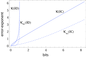
Note that we have already computed $Q$ for both the detectors. Thus, we can easily derive $\kappa=\kappa(\mu)$ and $\kappa_{loc}=\kappa_{loc}(\mu)$ for the coherent and incoherent detector, respectively. These quantities can then be expressed in terms of the encoded discord $\delta D$ and classical correlations $\delta C$. As shown in Fig. 5, there is a strict separation $\kappa>\kappa_{loc}$ for any non-zero value of the classical correlations.

Figure 5: Error-probability exponents, $\kappa$ (coherent detector) and $\kappa_{loc}$ (incoherent detector), plotted versus discord $\delta D$ (left curves) and classical correlations $\delta C$ (right curves). Note the strict separation $\kappa>\kappa_{loc}$ for any non-zero value of the correlations.

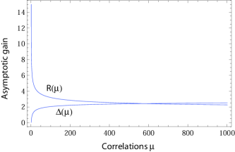
In order to better display the separation we consider the difference between the two error-exponents $\Delta:=\kappa-\kappa_{loc}$ which is directly plotted in terms of the parameter $\mu$. As we can see from Fig. 6, the gain $\Delta(\mu)$ is strictly positive and increasing in the correlations. In particular, we have $\Delta\rightarrow\Delta_{\max}>2$ for maximal correlations, i.e., for $\mu\rightarrow+\infty$ corresponding to $\delta D\rightarrow 1$ and $\delta C\rightarrow+\infty$. A similar improvement can be appreciated by considering the ratio $R:=\kappa/\kappa_{loc}\geq 1$ which converges to about $2$ dB for $\mu\rightarrow+\infty$. Thus, it is clear that the use of the coherent detector outperforms any incoherent detector based on the use of single-mode Gaussian measurements for the task of discriminating the presence or not of correlations in Gaussian states (both classical and quantum correlations).

Figure 6: Asympotical gain, both quantified as a difference $\Delta=\kappa-\kappa_{loc}$ and as a ratio $R=\kappa/\kappa_{loc}$, versus the encoded correlations $\mu$. Here $R$ is expressed in dB.

5 Conclusion and discussion

In this work, we have considered the discrimination of discord and classical correlations in two-mode separable Gaussian states, showing how non-local optimal detectors may retrieve strictly more information than local Gaussian detectors. This is true both in the setting of single- and multi-copy state discrimination. Potential extensions of the work may involve the use of asymmetric state discrimination, where the quantum Hoeffding bound [17] and the relative entropy [23] can be analytically computed over Gaussian states (e.g., see Theorem 6 in Pirandola et al. [24]). It would also be interesting to establish the actual performance of local but non-Gaussian detectors, and also to investigate the explicit implications for Gaussian data hiding.

Appendix A Symplectic decomposition of our two-mode covariance matrix

Consider a CM in the symmetric form

$$\mathbf{V}=\left(\begin{array}[c]{cccc}\mu&&g&\\ &\mu&&g\\ g&&\mu&\\ &g&&\mu\end{array}\right)~{},$$ (52)

with bona-fide conditions $\mu\geq 1$ and $\left|g\right|\leq\mu-1$, coming from Eq. (10). Since it is a real symmetric matrix, it can be reduced to a diagonal form $\mathbf{V}=\mathbf{ODO}^{T}$ by a proper rotation, i.e., a special orthogonal matrix $\mathbf{O}\in SO(4)$ ($\mathbf{O}^{T}=\mathbf{O}^{-1}$ and $\det\mathbf{O}=+1$). In particular, we have

$$\mathbf{O}=\frac{1}{\sqrt{2}}\left(\begin{array}[c]{cc}-\mathbf{X}&\mathbf{X}\\ \mathbf{X}&\mathbf{X}\end{array}\right),~{}\mathbf{X:}=\left(\begin{array}[c]{cc}0&1\\ 1&0\end{array}\right)~{},$$ (53)

and the diagonal form is composed of two degenerate eigenvalues

$$\mathbf{D}=\left(\begin{array}[c]{cc}(\mu-g)\mathbf{I}&\\ &(\mu+g)\mathbf{I}\end{array}\right)~{}.$$ (54)

It is easy to check that $\mathbf{O}$ is not symplectic. However, starting from $\mathbf{O}$, it is very easy to construct a symplectic matrix $\mathbf{S}$ such that

$$\mathbf{V}=\mathbf{SDS}^{T}.$$ (55)

In fact, it is sufficient to consider

$$\mathbf{S}=\mathbf{O}(\mathbf{Z}\oplus\mathbf{Z})~{},$$ (56)

where we have introduced the reflection matrix

$$\mathbf{Z}=\left(\begin{array}[c]{cc}1&\\ &-1\end{array}\right)~{}.$$ (57)

One can check that $\mathbf{S}$ preseves the symplectic form, i.e., $\mathbf{S}\boldsymbol{\Omega}\mathbf{S}^{T}=\boldsymbol{\Omega}$, with

$$\boldsymbol{\Omega}=\boldsymbol{\omega}\oplus\boldsymbol{\omega},~{}\boldsymbol{\omega}:=\left(\begin{array}[c]{cc}0&1\\ -1&0\end{array}\right)~{}.$$ (58)

Then, since $\mathbf{Z}^{2}=\mathbf{I}$, we have that the decomposition of Eq. (55) holds true. Thus, we have that $\mathbf{D}$ of Eq. (55) is Williamson’s normal form of the CM, with symplectic spectrum $\nu_{\pm}=\mu\pm g$, and $\mathbf{S}$ of Eq. (56) is the diagonalizing symplectic matrix. Setting $g=\mu-1$ we retrieve the same symplectic eigenvalues, $\nu_{-}=1$ and $\nu_{+}=2\mu-1$, given in the main text.

Appendix B Optimality of heterodyne

As we can see from Eq. (32) a single-mode Gaussian POVM is characterized by three parameters $\mathcal{G}=\mathcal{G}(\eta,\theta,\lambda)$. In our search for the optimal POCM, we can heuristically reduce the number of parameters from 3 to just $\lambda$ (a more rigorous proof of this reduction can be given, but it is omitted for brevity).

Note that the Gaussian POVM on mode $B$ has an effect on mode $A$ if and only the initial two-mode state is correlated ($\rho_{1}$), and its effect is the preparation of a randomly-displaced Gaussian state $\rho_{1}^{A|B}(\mathbf{a})$. This state has to be distinguished from a thermal state $\rho_{0}^{A}$, which is equal to averaging $\rho_{1}^{A|B}(\mathbf{a})$ averaged over the random modulation, i.e.,

$$\rho_{0}^{A}=\int d\mathbf{a}~{}G_{\tilde{V}}(\mathbf{a})\rho_{1}^{A|B}(\mathbf{a})~{}.$$ (59)

First of all, it is intuitive to understand that the optimal Gaussian POVM is rank-1, which corresponds to taking $\eta=1$. In fact, if we take $\eta>1$, we see from Eq. (33) that the modulation $\mathbf{\tilde{V}}$ decreases and, correspondingly, the conditional CM $\mathbf{V}_{A|B}$ increases (where the increase/decrease must be intended here as an increase/decrease in the symplectic eigenvalue or determinant). This clearly reduces the distinguishability of $\rho_{1}^{A|B}(\mathbf{a})$ from the average thermal state $\rho_{0}^{A}$.

Then, among the rank-1 Gaussian POVMs $\mathcal{G}(1,\theta,\lambda)$, no angle $\theta$ is preferred. In fact, if $\lambda=1$ (heterodyne) we have that any rotation in Eq. (32) is equivalent to the identity. If $\lambda\neq 1$, the measurement remotely prepares a displaced thermal state which is squeezed and rotated by $\theta$. However, since the alternative state ($\rho_{0}^{A}$) is isotropic in phase space, there is no advantage in preparing states which are squeezed in a particular direction.

Thus, we are left with rank-1 Gaussian POVMs of the form $\mathcal{G}(1,0,\lambda)$ and we want to prove that the optimal is achieved by $\lambda=1$. To prove this, let us consider $\rho_{1}$ having a more general CM, given by the blockform

$$\mathbf{V}_{1}=\left(\begin{array}[c]{cc}\mu\mathbf{I}&g\mathbf{I}\\ g\mathbf{I}&\mu\mathbf{I}\end{array}\right)~{},$$ (60)

with $\left|g\right|\leq\mu-1$. In this case, we derive two diagonal matrices

$$\mathbf{\tilde{V}}=g^{2}\left(\begin{array}[c]{cc}\frac{1}{\lambda+\mu}&\\ &\frac{1}{\lambda^{-1}+\mu}\end{array}\right)~{},$$ (61)

and

$$\mathbf{V}_{A|B}=\mu\mathbf{I}-\mathbf{\tilde{V}}=\left(\begin{array}[c]{cc}d_{+}&\\ &d_{-}\end{array}\right)~{},$$ (62)

with

$$d_{\pm}:=\mu-\frac{g^{2}}{\lambda^{\pm 1}+\mu}~{}.$$ (63)

Then, we can write the symplectic decomposition $\mathbf{V}_{A|B}=\nu_{A|B}\mathbf{SS}^{T}$, where $\nu_{A|B}=\sqrt{d_{+}d_{-}}$ and

$$\mathbf{S}:=\left(\begin{array}[c]{cc}\sqrt[4]{\frac{d_{+}}{d_{-}}}&\\ &\sqrt[4]{\frac{d_{-}}{d_{+}}}\end{array}\right)~{}.$$ (64)

Next, we compute the quantities involved in the $s$-overlap, i.e.,

$$\Pi_{s} =2G_{s}(\mu)G_{1-s}\left(\sqrt{d_{+}d_{-}}\right)$$ (65)

$$\boldsymbol{\Sigma}_{s} =\Lambda_{s}(\mu)\mathbf{I}+\Lambda_{1-s}(\sqrt{d_{+}d_{-}})\mathbf{SS}^{T}\text{.}$$ (66)

Thus, by replacing Eqs. (61), (65) and (66) into Eq. (41), we get $Q_{s}=Q_{s}(\mu,g,\lambda)$. This expression is analytical as well as its first derivative $\frac{\partial Q_{s}}{\partial\lambda}$. One can check that $\lambda=1$ is a critical point and represents a global minimum for any allowable value of $s$, $\mu$ and $g$. In particular, this is true for $g=\mu-1$.

References

• [1] J. Watrous, The theory of quantum information (Cambridge University Press, Cambridge, 2018).
• [2] M. Hayashi, Quantum Information Theory: Mathematical Foundation (Springer-Verlag Berlin Heidelberg, 2017).
• [3] M. A. Nielsen and I. L. Chuang, Quantum Computation and Quantum Information (Cambridge University Press, Cambridge, 2000).
• [4] C. Weedbrook et al., Rev. Mod. Phys. 84, 621 (2012).
• [5] A. Holevo, Quantum Systems, Channels, Information: A Mathematical Introduction (De Gruyter, Berlin-Boston, 2012).
• [6] H. Ollivier and W. H. Zurek, Phys. Rev. Lett. 88, 017901 (2001).
• [7] L. Henderson and V. Vedral, J. Phys. A 34, 6899 (2001).
• [8] K. Modi, A. Brodutch, H. Cable, T. Paterek, and V. Vedral, Rev. Mod. Phys. 84, 1655-1707 (2012).
• [9] G. Adesso and A. Datta, Phys. Rev. Lett. 105, 030501 (2010).
• [10] P. Giorda and M. G. A. Paris, Phys. Rev. Lett. 105, 020503 (2010).
• [11] S. Pirandola, G. Spedalieri, S. L. Braunstein, N. J. Cerf, and S. Lloyd, Phys. Rev. Lett. 113, 140405 (2014).
• [12] D. P. DiVincenzo, D. W. Leung, B. M. Terhal, IEEE Trans. Inf Theory 48, 580-599 (2002).
• [13] C. W. Helstrom, Quantum detection and estimation theory (Academic Press, New York, 1976).
• [14] K. M. R. Audenaert et al., Phys. Rev. Lett. 98, 160501 (2007).
• [15] S. Pirandola and S. Lloyd, Phys. Rev. A 78, 012331 (2008).
• [16] S. Pirandola, A. Serafini, and S. Lloyd, Phys. Rev. A 79, 052327 (2009).
• [17] G. Spedalieri, and S. L. Braunstein, Phys. Rev. A 90, 052307 (2014).
• [18] J. Williamson, Am. J. Math. 58, 141 (1936).
• [19] S.-H. Tan et al., Phys. Rev. Lett. 101, 253601 (2008).
• [20] In general, consider a two-mode Gaussian state ρA​Bsubscript𝜌𝐴𝐡\rho_{AB} with zero mean and CMΒ
𝐕=(𝐀𝐂𝐂T𝐁).𝐕𝐀𝐂superscript𝐂𝑇𝐁\mathbf{V}=\left(\begin{array}[c]{cc}\mathbf{A}&\mathbf{C}\\ \mathbf{C}^{T}&\mathbf{B}\end{array}\right)~{}.
By performing a local Gaussian POVM (𝐕σsubscriptπ•πœŽ\mathbf{V}_{\sigma}) on mode B𝐡B with outcome 𝐱𝐱\mathbf{x}, we prepare a randomly-displaced Gaussian state on mode A𝐴A, with displacement 𝐚=πšβ€‹(𝐱)𝐚𝐚𝐱\mathbf{a}=\mathbf{a}(\mathbf{x}) and conditional CM 𝐕A|B=π€βˆ’π•~subscript𝐕conditional𝐴𝐡𝐀~𝐕\mathbf{V}_{A|B}=\mathbf{A}-\mathbf{\tilde{V}} with
𝐕~:=𝐂​(𝐁+𝐕σ)βˆ’1​𝐂T.assign~𝐕𝐂superscript𝐁subscriptπ•πœŽ1superscript𝐂𝑇\mathbf{\tilde{V}}:=\mathbf{C}(\mathbf{B}+\mathbf{V}_{\sigma})^{-1}\mathbf{C}^{T}~{}.
Note that 𝐕~~𝐕\mathbf{\tilde{V}} is a classical CM which describes the random modulation of the state. In fact, summing this CM to the conditional CM, i.e., 𝐕~+𝐕A|B~𝐕subscript𝐕conditional𝐴𝐡\mathbf{\tilde{V}+V}_{A|B}, we get exactly the quantum CM 𝐀𝐀\mathbf{A}, which describes the average state on mode A𝐴A, i.e., the reduced state ρA=TrB​(ρA​B)subscript𝜌𝐴subscriptTr𝐡subscript𝜌𝐴𝐡\rho_{A}=\mathrm{Tr}_{B}(\rho_{AB}).
• [21] H. Scutaru, J. Phys. A 31, 3659 (1998).
• [22] L. Banchi, S. L. Braunstein, and S. Pirandola, Phys. Rev. Lett. 115, 260501 (2015).
• [23] S. Pirandola, R. Laurenza, C. Ottaviani, and L. Banchi, Nat. Commun. 8, 15043 (2017).
• [24] S. Pirandola, S. L. Braunstein, R. Laurenza, C. Ottaviani, T. P. W. Cope, G. Spedalieri, and L. Banchi, Quantum Sci. Technol. 3, 035009 (2018).